Article

Algorithm Fusion for 3D Ground-Penetrating Radar Imaging with Field Examples

1
Department of Earth Sciences, National Taiwan Normal University, 88, Sec. 4, Ting-Chou Road, Taipei 116, Taiwan
2
New Taipei Municipal SanMin High School, New Taipei City 247, Taiwan
3
National Lo-Dong Senior High School, Yilan 265, Taiwan
*
Author to whom correspondence should be addressed.
Remote Sens. 2023, 15(11), 2886; https://doi.org/10.3390/rs15112886
Submission received: 28 March 2023 / Revised: 12 May 2023 / Accepted: 29 May 2023 / Published: 1 June 2023

Abstract

:
Numerous data processing algorithms are available for ground-penetrating radar (GPR) data processing. However, most of the existing processing algorithms are derived from Fourier theory and assume that the system is linear or that data are stationary, which may oversimplify the case. Some nonlinear algorithms are accessible for improvement but generally are for stationary and deterministic systems. To alleviate the dilemma, this study proposes an algorithm fusion scheme that employs standard linear techniques in conjunction with a newer nonlinear and non-stationary method. The linear techniques include linear filtering, migration, and interpolation. The newer method is mainly for nonlinear filtering and image reconstruction. The results can be demonstrated in a two-dimensional single profile (time–distance section) or a 3D visualization if survey lines fulfill the 3D Nyquist sample intervals requirement. Two controlled experiments were conducted to justify the proposed scheme. Then, a field study including two examples was carried out to demonstrate the feasibility of practical applications. Compared with conventional methods, the proposed algorithm fusion provides better visualization and integrative interpretation for GPR imaging.

1. Introduction

In scientific and engineering investigations, various techniques are available for non-destructive testing (NDT) and earth observation (EO). Ground-penetrating radar (GPR) is one of the essential geophysical techniques practiced in these fields [1,2,3,4]. The advantages of using GPR are its versatility in detecting targets, regardless of metallic or nonmetallic nature [3], with low cost, high resolution, and real-time imaging [5,6].
To carry out a successful GPR survey, data processing is crucial, and effective algorithms or appropriate processing schemes certainly help. In the past few decades, numerous data processing algorithms have been proposed to improve outcomes in GPR imaging. There are commonly two categories, i.e., data analysis and simulation. This study focuses on data analysis.
As is well known, linearity (system satisfies the superposition principle) and stationarity (data features are constant over time) are two major concerns when processing real-world data. For linear and stationary processing, Fourier analysis and Fourier transform are well-developed robust approaches, and therefore several Fourier-based novel algorithms are available. Among them, wavelet transform [7], multiresolution analysis (MRA) [8], curvelet filtering [9], and singular value decomposition (SVD) [10] are popular for noise suppression of non-stationary data under some fundamental restrictions similar to Fourier transform. For example, wavelet transformation and its related approaches [11,12] postulate that the system is linear, and the data must be periodic or stationary [13]. In fact, all the other algorithms mentioned above assume, or at least do not reject, that the systems are linear when processing non-stationary data, but this is rarely the case for real data. Most systems are usually nonlinear and data are non-stationary. Other than the data analysis approaches, an optimized modeling technique, the full waveform inversion [14,15,16] method, is suggested for improving GPR image resolution. Moreover, some innovative machine learning approaches using statistical methods and neural network mathematical models [17,18,19] have evolved in recent years. Optimized modeling and simulation techniques provide alternative solutions, but those are akin to a popular seismological method called evolutionary spectrum [20] and the applications may change data analysis into statistical data simulation [21], which is outside the scope of this study.
For nonlinear data processing, several nonlinear time-series analysis methods are accessible [22,23] but assume the systems are stationary and deterministic [24,25], which is unrealistic because an a priori basis creates more problems than solutions [26].
Although having limitations in application, most existing methods of data analysis can basically deal either with linear nonstationary or nonlinear stationary data processing but have difficulty in performing nonlinear and nonstationary data analysis.
In this study, we aim to propose an algorithm fusion scheme to alleviate the dilemma of processing nonlinear and nonstationary data. The conventional (called “standard” as well) and novel algorithms all have their advantages and shortcomings. Most conventional algorithms are theoretically complete and authentic in technical applications, even though they may not be perfect. The novel algorithms can cope with nonlinear and nonstationary problems but usually suffer from incomplete theory, confidence limit, and high computation cost. Therefore, a decent fusion of conventional and contemporary algorithms may provide a better solution. For this reason, we designed an algorithm fusion scheme that combines a nonlinear and nonstationary data analysis method with conventional Fourier-based algorithms. The nonlinear and nonstationary algorithm, natural logarithmic transformed (NLT) ensemble empirical mode decomposition (EEMD), is a modified empirical mode decomposition (EMD) method with a noise-assisted extension. The conventional algorithms are standard GPR processing techniques including background noise removal filters at the beginning of processing, frequency-wavenumber (fk) migration to focus GPR images, and 2D time slice interpolation in the pseudo-3D data construction. We designed two control experiments, including 2D profiling and 3D imaging, to assess the proposed method before carrying out a field survey. An archaeological site located in a remote mountainous village was selected as the site for the case study. The proposed method shows significant advantages, both in the experiments and in the case study.

2. Materials and Methods

Since the 1970s onwards, GPR is a reflection technique that has become more popular for high-resolution near-surface EO in geophysics with links to NDT [5,27]. However, GPR data usually need a skillful process to develop a meaningful profile (time–distance section) for interpretation. To acquire a desired high-resolution GPR image, signal attenuation and noise interference are two main issues to solve. The higher-level goal is to achieve full-resolution 3D imaging. Time slices of the 3D data volume allow the interpreter to generate contour maps for different horizons. Therefore, a better image of buried targets can be obtained from the contour maps of a 3D GPR data volume. Although both field techniques and commercial software for 3D GPR surveys have been available for decades, researchers are still making efforts to improve the quality and efficiency of 3D GPR field surveys [28,29,30,31]. A particular focus is on rugged terrain and places with vegetation. The situation could be more difficult for employing 3D techniques in some special environments such as potential archeological sites, due to the requirements of cultural heritage preservation. To deal with the mentioned challenging tasks and make better GPR imaging possible, we propose an algorithm fusion scheme with experiments and field examples in the hope of making it a valuable tool for future GPR studies. In the experiments, we separated 2D and 3D considerations into different controlled tests because 2D imaging is still the most practiced technique in the field, and the proposed method is not only effective for 3D imaging. The field study aimed to investigate a cultural protection archaeological site with dense vegetation that might prohibit laying out full-resolution 3D survey lines. Therefore, we designed a casket model to carry out 2D imaging in the first experiment and tested the 3D imaging of a miniature multilayered archaeological object model with extremely limited survey lines in the second experiment to evaluate the proposed method before conducting the field study. The rest of this section describes the details of the proposed fusion scheme.

2.1. Standard Linear Process

Original GPR data may suffer severely from systemic and environmental noise. Before applying the nonlinear method, we adopt common linear filtering techniques for preliminary data processing because the techniques are well-developed and effective for simple routine processing. These include a de-pulse filter to mute abnormal peaks, a de-DC (vertical background removal) filter to remove temporally consistent noise, e.g., system noise or locally superposed diffraction energy, and a de-mean (horizontal or sliding background removal) filter to subtract the horizontally coherent noise from the data. All the techniques mentioned are available In common textbooks [32,33] and commercial GPR data processing software, e.g., REFLEXW (K.J. Sandmeier Zipser Straße 1 D-76227 Karlsruhe Germany) and Matlab (a product of the MathWorks, Inc., Natick, MA, USA). However, to connect with our nonlinear processing procedure efficiently, we created a Matlab script for the preliminary linear process.

2.2. Nonlinear and Nonstationary NLT EEMD Filter Bank

EEMD, or its earlier version EMD, is an empirically based adaptive nonlinear data-analysis method. The filter bank derived from the EMD or EEMD analysis is dyadic, which indicates a collection of band-pass filters that decomposes the input data into multiple components, and the spectra of neighboring filters can be overlapped [34]. The theoretical investigation and applications of EMD or EEMD and related analysis methods are still evolving. Numerous reports are available in the literature [35,36,37,38,39,40,41,42,43,44,45,46,47,48]. We summarize EEMD’s technical details in the Appendix A for readers who do not specialize in this subject.
Unlike those using mono-frequency and stationary harmonic functions as the basis, the components derived from the EMD/EEMD filter bank are “oscillating functions” called intrinsic mode functions (IMFs). IMFs must satisfy two conditions: (1) The number of extrema and the number of zero crossings must be equal, or differ at most by one; (2) the envelopes defined by the local maxima and local minima are symmetrical to zero [21,25]. IMFs, therefore, represent the significant physical oscillation modes embedded in the data [21,38]. As a consequence, the filter bank provides a new means of nonlinear filtering to extract the signal and eliminate the noise from GPR data [49].
EEMD is a noise-assisted EMD algorithm. This approach effectively reduces mode mixing and is a substantial improvement over the EMD method. While EEMD yields an effective way of enhancing the signal and has fewer mode mixing problems than EMD, the energy dissipation caused by intrinsic attenuation and geometric spreading in GPR data is still a major factor that affects the success of EEMD filtering. One way to avoid distorting the data attributes when compensating for energy dissipation is by applying NLT to the amplitude of the data before EEMD [49]. The conversion is simply to take the natural logarithmic transform of the attenuated signal y(t) as
Ly(t) = sign [slog(c +│y(t)│)]
where Ly(t) is the logarithm of the signal y(t); sign is the sign function for keeping the signal’s original polarity, which is defined as 1 for y(t) > 0, 0 for y(t) = 0, and −1 for y(t) < 0 [45]. The constant c is to make the logarithmic value positive; the scaling factor s is the maximum output value control. NLT just displays signals on a logarithmic scale, and amplitude values are intact.
This conversion operation is not a conventional practice in GPR data processing; it is similar to the well-known techniques of the dB scale in acoustic engineering and the Richter scale in seismology. NLT resembles the coordinate transformation commonly undertaken in mathematical physics. The proper choice of scale or reference system enhances the signal, and more importantly, the correlations and physical facts of the data do not depend upon which coordinate system or scale we use. Based on the reasons stated above, the logarithmic scale improves the dynamic range, i.e., permits a wider range of values than the linear scale when displaying data on the amplitude axis, and causes no artificial distortion [49,50].
A valuable application of the NLT EEMD filter bank is to reconstruct data. When reconstructing data, investigators should have fundamental knowledge of the signal and noise attributes in the data, and make basic assumptions for selecting components [38]. Since the patterns of signal and noise in reflection data are usually discernable and easy to identify, it is simple to reconstruct the data. The procedure is first to decompose each single GPR trace into a finite number of IMFs, and then to select components with convincing physical significance for 1D trace reconstruction. As a result, an EEMD-filtered 2D GPR profile is a collection of filtered 1D traces acquired from 2D survey lines, and a 3D volume is the combination of filtered 2D profiles with equal spacing. If the 2D survey line spacing and trace spacing are too coarse to achieve the Nyquist sample interval, or the two spacings are not equal, interpolation is required.

2.3. Algorithm Fusion and Construction of 3D Visualization

There are numerous algorithms available for GPR data processing. Most of them are effective under certain conditions. In this study, we try to integrate decent algorithms from various sources to achieve a better methodology for 3D GPR data processing that is difficult or not feasible using a specific processing system. It is well-known that filtered 2D data may construct a 3D cube if the original data are well-sampled, i.e., densely deployed parallel 2D lines of equal spacing with a high temporal sampling rate in one direction or, even better, in two perpendicular directions. Certainly, some conventional GPR processing steps (i.e., linear filtering, migration, etc.) are useful before or after 3D data construction. The constructed 3D cube can be re-interpolated (further interpolated) to increase sampling density if the data density in a certain direction is not high enough for presenting a satisfactory 3D cube or to compare two different 3D data files that were acquired in two different directions. These procedures are vital in depicting the data features. In the proposed algorithm fusion, we apply the conventional fast Fourier transform interpolation (FFTI) approach to pad zeros at higher frequencies of the Fourier coefficient vector, thus yielding more points in the time domain and producing the effect of interpolation [51].
Figure 1 is a flowchart indicating both the standard process flow and the proposed algorithm fusion sequence. The fusion strategy in this study is an integration of conventional GPR data processing techniques with the NLT EEMD method. At first, standard background noise-removing filters (de-pulse, de-DC, de-mean, etc.) are applied to eliminate temporally consistent noise (vertical noise) and spatially coherent noise (horizontal noise) from the data, and then each GPR trace is transformed into log scale by implementing NLT to reduce the exponential decay of the original data. As the major contribution of NLT is to compensate for energy dissipation, it may exaggerate horizontal coherent events. Therefore, it must be performed before EEMD but not necessarily before horizontal background noise removal. In practical GPR data processing, NLT can be performed before or after horizontal background noise removal.
EEMD filtering is a key procedure to enhance the signal by removing noise components and reconstructing the data using components of significant events. Depending on the distribution of signal events within the decomposed components, a reconstructed 2D profile could comprise one or several components. The EEMD-filtered 2D profiles are then ready for interpretation or generating a 3D file directly, as long as the original data are well-sampled. Usually, if the stated condition fails, interpolations are required before 3D data volume construction, and the result is a pseudo-3D image.
When using EEMD techniques, we first decompose each single GPR trace into a finite number of IMFs by using the NLT EEMD filter bank. With basic knowledge of reflection methods (GPR or seismic), one can easily distinguish the noise/signal events and then extract components with convincing physical significance for 1D trace reconstructing and 2D profiling (a good example will be shown in Section 3.1.2). However, some tricky fake events (see Section 3.1.1) may need further analysis such as velocity analysis, modeling, spectral analysis, and so on. We prefer to adopt marginal spectrum analysis, which was successfully applied in several of our studies [6,45,49]. Since this technique has been widely applied in many subjects and the aim of this paper does not focus on this topic, we briefly mention it and give references. Marginal spectrum analysis is also vital for conventional filtering to determine the pass-band of the filter, as will be shown and justified in the later section.
In general, an NLT EEMD-filtered 2D GPR profile is a collection of NLT EEMD-filtered 1D traces acquired from 2D survey lines, and a 3D volume is the integration of NLT EEMD-filtered 2D profiles of equal spacing with interpolation as needed. NLT EEMD filtering can be multidimensional if the computation cost is affordable.

3. Results

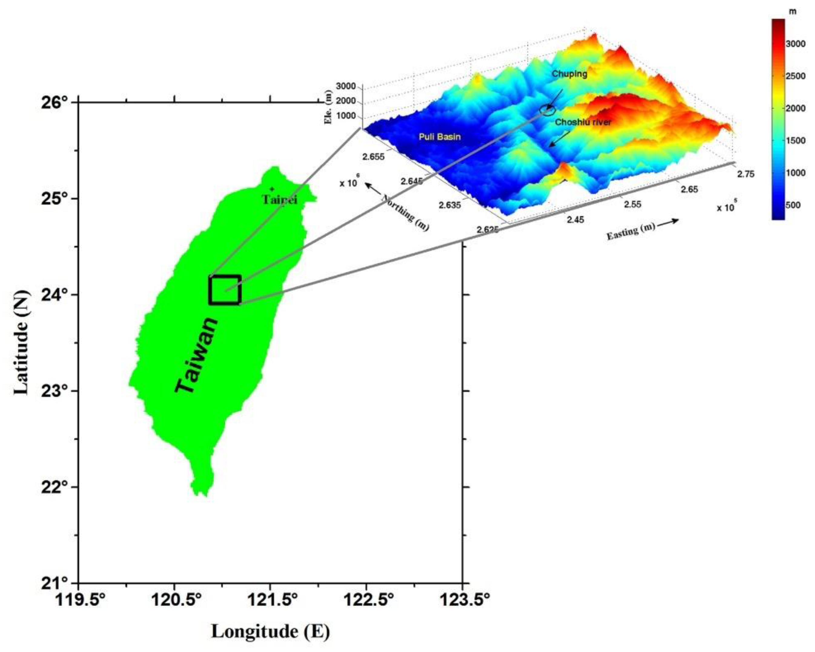
We carried out two controlled experiments followed by two field examples for assessing the feasibility of applying the proposed algorithm fusion to GPR field investigation. The experimental site was located within a university recreation park near a riverbank. It was a riverside farm field before it became a park. The field site was on the Chuping archaeological site in central Taiwan (Figure 2), which is also close to a river. Therefore, the sedimentary environments and the soil at both sites are comparable. However, due to construction, the surface at the experimental site is paved with a thin layer of waste dump soil together with the unconsolidated layers of silt, sand, and gravel underneath. In addition, the water table at the experimental site is always higher because of the weather. These factors make the experimental site a place of poor reflection quality [52], and a challenging environment for conducting GPR experiments.

3.1. Controlled Experiments

To validate the proposed algorithm fusion, we demonstrate two controlled experiments. The first experiment focuses on a 2D test while the second experiment is to examine 3D imaging.

3.1.1. 2D Algorithm Experiment

The survey target was a brick casket model (1.0 m × 0.40 m × 0.35 m), originally buried in the park about 80–85 cm below the surface for geophysical experiments since 2002 (Figure 3a). It has been utilized to perform magnetic and seismic studies and has shown challenging geophysical attributes [53,54]. The casket model was made of dry stacked construction bricks (0.20 m × 0.092 m × 0.05 m). The lid and bottom of the casket model were composed of a single layer of 0.05 m thick bricks. The four 0.092 m thick walls were stacked up with the bricks horizontally. Previously excavated soil materials (silt, sand, and gravel) were mixed to fill up the space inside the casket model and then also used for backfilling. The disturbed soil materials were initially less dense, and then gradually become more compact over time. Moreover, the park was re-landscaped by the university after the model was buried. Therefore, the depth of the casket model could be altered. Another interfering factor in this experiment is that the experiment was conducted soon after a severe flooding event. The water table was close to the ground surface due to heavy rainfall in previous days. Although the environment was not suitable for GPR surveying, it was a keen test for the proposed method. In this experiment, we acquired data from several E–W survey lines using a shielded 500 MHz GPR system. The acquisition parameters were set to 0.052 ns temporal sample intervals for 1024 samples per trace, and 0.018 m spatial sample interval on the survey line to avoid in-line aliasing. A typical survey line, EW09 (Figure 3b), was selected for demonstrating the proposed processing technique. The soil auger-pricking probe (Figure 3c) after GPR imaging confirmed that the depth was between 0.8 m and 0.85 m.
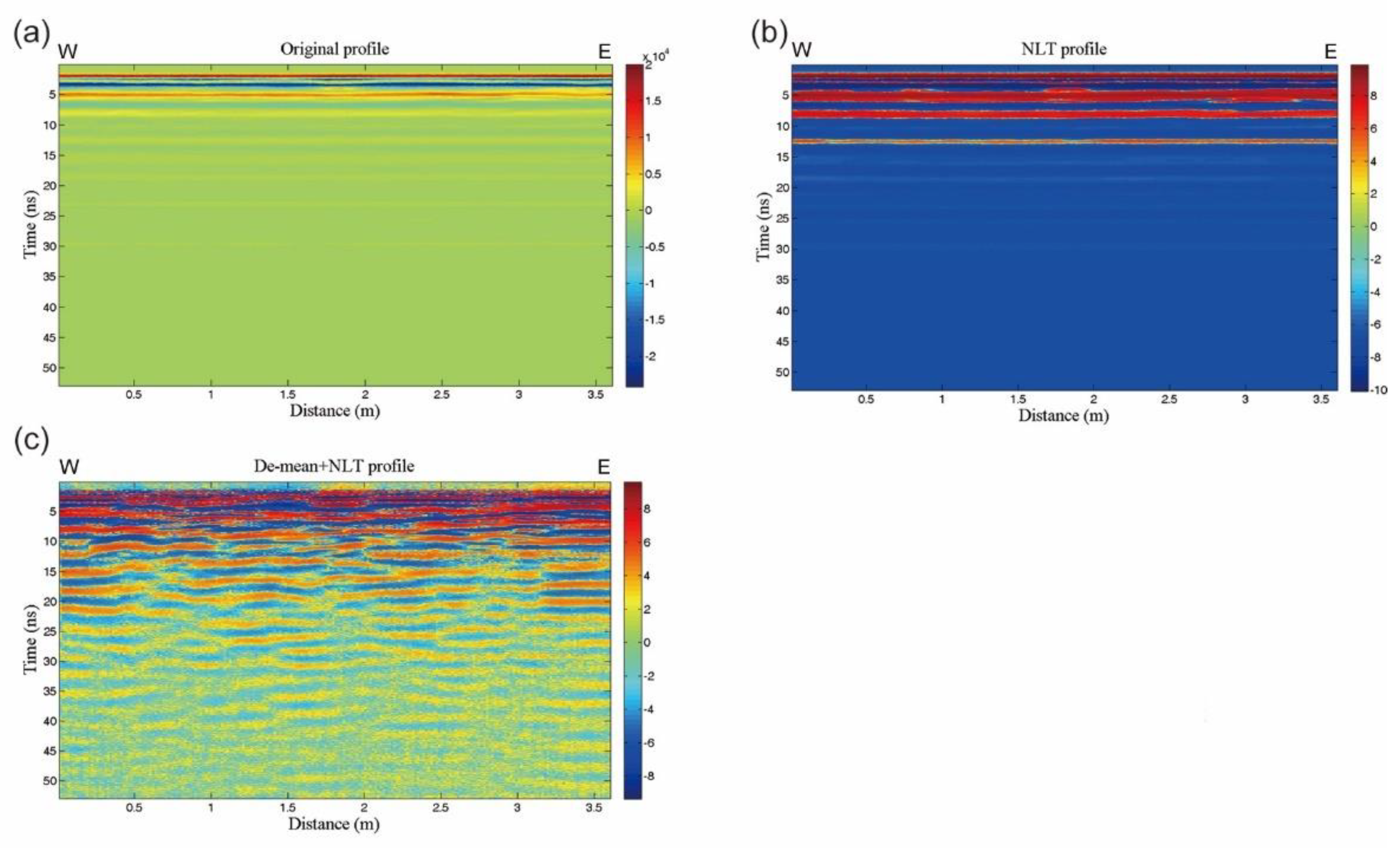
Figure 4a shows the original profile of EW09 after the removal of vertical noise (abnormal pulses and the DC bias). In this profile, the airwave, direct wave, and strong water table reflection with multiples masked the deeper reflections. The penetration depth only reached about 5 ns. After the NLT process, the penetration depth extended to about 14 ns but no significant reflections were present (Figure 4b). Apparently, the interference of strong horizontally coherent noise generated by the water table was a major factor. Therefore, we employed the linear horizontal filtering technique, which applies a de-mean filter to subtract the horizontally coherent noise from the data. After de-mean filtering, the horizontally coherent noise was collapsed to reveal the deeper image, and the resolution of the NLT profile was significantly improved (Figure 4c). The next procedure was to carry out the nonlinear filtering technique (EEMD) vertically, i.e., to decompose each trace of the de-mean + NLT profile shown in Figure 4c. In this case, each GPR trace in the profile of Figure 4c was decomposed into eleven IMF components of different frequency bands to establish the trace filter bank (traces of different frequency bands). After examination, we selected the four most meaningful IMF components, C3, C4, C5, and C6. The next step was to try out the best combination of the four components.
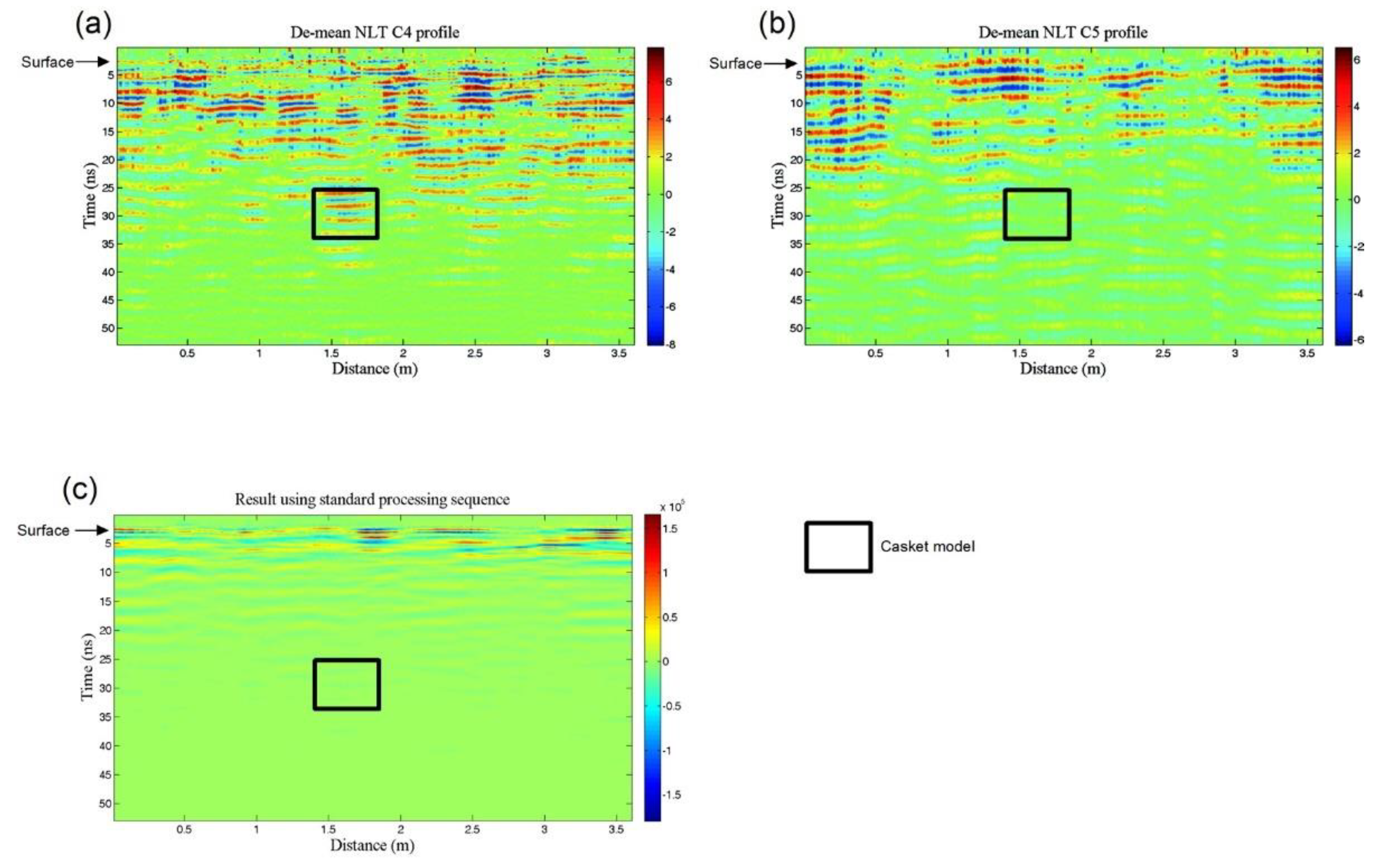
Through comparing the results for using each component and different combinations of various components for reconstruction, we determined that using only component C4 to reconstruct the trace would obtain the best NLT EEMD filtered profile as a result (Figure 5b). Figure 5a,c, and d are the NLT EEMD filtered profiles using components C3, C5, and C6, respectively. Note that the model reflection energy is concentrated in component C4; the higher frequency component C3 (Figure 5a) has no event correlated to the model, while the lower frequency component C5 shows a blank window at the inferred buried casket model position (Figure 5c). The profile constructed using C6 is dominated by low-frequency noises. In this study, it happened that a single-component reconstruction outperformed multi-component combinations. Many cases that we have dealt with in other fields of study are the combination of more than one component. A single-component reconstruction is not a typical case. One component taking it all happened accidentally in this study. A possible reason is that the feature of the signal is relatively unique and resides in only one component. As EEMD effectively removes mode mixing, a single-component reconstruction is conceivable.
For comparison, the original profile (Figure 4a) was also processed using a conventional processing scheme. We employed a gain function to compensate for energy loss, background removal to suppress horizontal coherent noise, and a band-pass filter to enhance the signal. The result is shown in Figure 6c. Before processing, we performed a model study on the shielded 500 MHz GPR system that we used in the experiment. The gain function g(t) consists of a linear and an exponential part:
g(t) = (1 + αt)eβt
We assumed the attenuation function for the model trace to be  e 20 t  [49] and inputted initial values of α = 1 and β = 10 to invert the final values for g(t). Of course, we could use a stronger gain function or use the AGC (auto gain control) commonly adopted in seismic data processing, but this could distort the original signal and cause a spectral shift, resulting in fake events [55].
It is also important to note that we determined the optimal pass-band of the conventional band-pass filter by analyzing the spectrograms of the EEMD components [56]. Comparing Figure 6a with Figure 6c, the proposed scheme outperformed the conventional method.

3.1.2. 3D Imaging Experiment

Non-destructive 3D GPR imaging is vital in detecting shallow targets. Even though both innovative field techniques and software for real 3D surveys are available in reflection seismology for exploring deep structures, such advanced methods may not be appropriate for shallow subsurface imaging in GPR investigation [29,56,57,58], particularly in rugged terrain and places with dense vegetation. Besides, the extra effort required for collecting full-resolution 3D field data [29] and much higher costs for handling large 3D data volumes may discourage GPR investigators. To confront this dilemma, we designed an experiment to show the possibility of keeping the acquisition effort at a reasonable level. The experimental target was a miniature model containing two buried DVD drives of different lengths to simulate multilayered historical objects or stacked tombs that may exist in our predetermined field area, the Chuping archaeological site. The longer DVD drive (20 cm ×14.2 cm × 4 cm) was buried right above the shorter one (16 cm × 14.2 cm × 4 cm). The shallower depth and deeper depth were 0.15 m and 0.45 m, respectively (Figure 7). A 1.0 m × 1.0 m grid was laid out over this experimental site with two sets of orthogonal GPR survey lines (Figure 7). The spacing between survey lines was 0.05 m; therefore, a total of 42 survey lines (21 E–W lines and 21 N–S lines) were deployed. In this experiment, a high-frequency one-piece MALA GeoScience shielded 1.2 GHz GPR system mounted on a small wheel carriage was employed to acquire the data. The recording parameters of this experiment were a 0.065 ns temporal sample interval for 512 samples per trace and a 0.01 m spatial sample interval on each survey line to fulfill the resolution criteria and mitigate spatial aliasing.
A typical E–W survey line (T12) in Figure 7 is demonstrated as an example. Following the processing sequence stated earlier, the original profile was decomposed into 9 components using the EEMD method. The major components (C1 to C6) are shown in Figure 8.
In this 3D imaging section, we changed the font of the component number to a subscript to avoid confusion with the symbols used in the 2D algorithm. With the help of logarithmic transform, the decomposed components were easy to classify as noise or signal. Despite the interference of background noise, the C2 component still accurately resolved the two buried targets of different lengths at different depths. Thus, in this case, only C2 of the EEMD decomposed components was recognized as the signal and selected for reconstructing the 2D profile. The events at 7 ns and 11 ns indicate the two buried DVD targets. Alternative reconstruction of the data can be performed by adding one more component, but no significant difference was observed in this case.
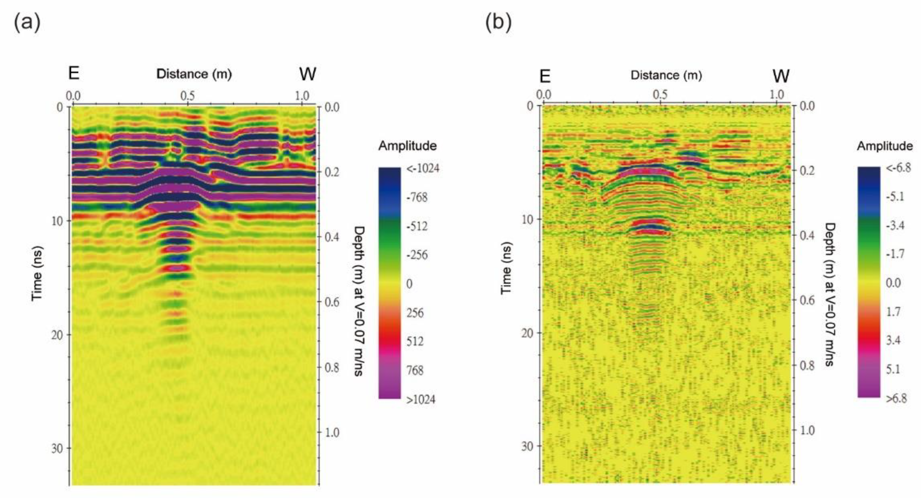
For comparison, Figure 9a,b show 2D profiles obtained by the conventional method (background noise removal plus band-pass filtering) and the proposed algorithm fusion method (background removal and NLT EEMD), respectively. The typical bandwidth of a 1200 MHz center frequency GPR system is between 600 MHz and 1800 MHz based on the −3 dB criterion. Optimum band-pass filtering in conventional processing can be achieved by simple tryout (iteration) or by spectral analysis. The 400–1000 MHz window simply refers to the results of spectral analysis. It is lower than the center frequency of the radar, which is possible because we dug a hole to bury the model and the previously excavated soil materials (silt, sand, and gravel) were used for backfilling. The unconsolidated dump materials attenuate much of the energy of higher-frequency radar waves, resulting in lower-frequency reflections. Nevertheless, the results shown in Figure 9 are effective in demonstrating the good performance of EEMD compared to conventional processing.
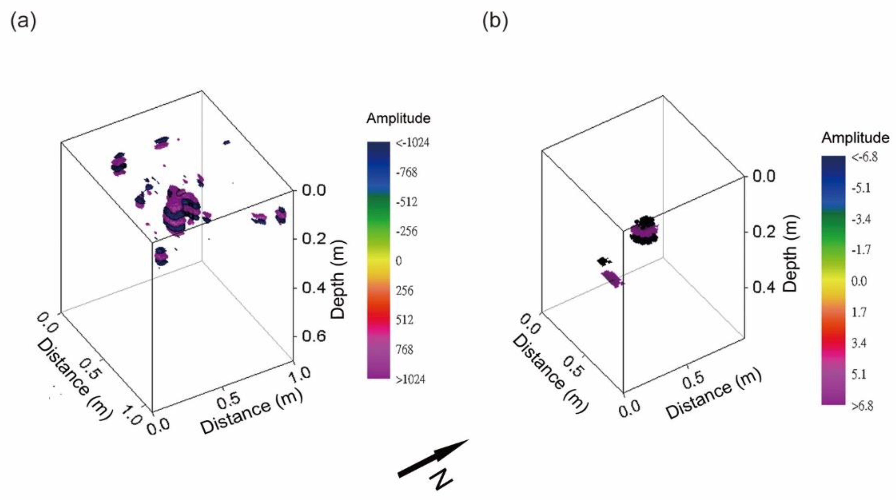
With success in processing 2D profiles, we extended the image to a 3D display. An image constructed using all 21 N–S survey lines with conventional processing sequence is shown in Figure 10a. To test the possibility of minimizing the field survey lines, we then took the data of just three N–S survey lines (L1, L11, and L21 in Figure 7) in this model study to construct the 3D image. Notice that only L11 traverses the subsurface target. With high interpolation, ten equally spaced lines were interpolated between the two survey lines, and the EEMD processed pseudo-3D data set revealed a more convincing image (Figure 10b) of the buried two DVD targets than that constructed by 21 N–S survey lines with conventional processing sequence. This outcome indicates that the proposed approach may significantly reduce field endeavors. However, the purpose of trying extremely few scans is to cope with very difficult environments such as dense vegetation, rugged terrain, and the most troublesome sites, such as a cultural heritage area where investigators are not allowed to lay out their survey lines however they need. Therefore, trying to use as few scans as possible is necessary, although it may be problematic, particularly if the target does not lie below one of the scans. Therefore, using extremely few scans is a compromise if an acceptable field layout is impossible. Examining our result, as long as one survey line crosses the target, the difficult environment seems not to be too distressing. With more endeavors, better solutions should be accessible.

3.2. Field Example from the Chuping Archaeological Site

Our field study area, the Chuping archaeological site, is located in a remote mountainous village. It is probably the most comprehensive high-altitude (924 m) prehistoric archaeological site documented in Taiwan to date. The site was a terrace farm before archaeologists developed an interest in this area, and it has been known to be a terrain of archaeological importance since the early 1980s when prehistoric stoneware was exposed on the hill slope [59]. Initiated in 1981, the Chuping archaeological site was excavated and investigated for seven years (1981–1987) by archaeologist Chung-Yu Chen to study the buried remains of a prehistoric settlement of highland Taiwanese aborigines in the upper valley of the Choshiu River. The excavated archaeological site was backfilled to preserve cultural heritage after the project was terminated, but the complete features of the Chuping archaeological site are still unclear. Thus, the history of this broad-scale prehistoric heritage is an interesting topic for further investigation. In addition, the Chuping archaeological site is probably multilayered and extends outside the excavated area due to its long period of settlement history. Therefore, assessment for deeper and broader re-excavation via a nondestructive method is still a research topic worth investigating further.
Figure 11a is a sketch that indicates the survey locations on the Chuping archaeological site where the backfilled area is surrounded by metallic grid fences. Two GPR survey squares shown in this subplot, the backfilled survey square (red square inside the fence) and the incomplete excavation survey square (outside the north end of the fenced area), were the places selected to test our proposed technique in practical archaeological investigation. Within the fenced area, the remains of ancient house foundations were frequently discovered along with slate caskets in the subsurface during the 1980s excavation [59]. This finding is quite unusual, judging from the present customs of Taiwanese indigenous peoples. One possible explanation for this is that the customs changed over time. Many of the ancient aboriginal tribes in Taiwan retained the custom of burying naturally deceased family members in the house to respect their souls and to continue family life with them [60].
At the time of the survey, the entire area was a field without any indication of the subsurface foundations and caskets. Figure 11b shows the landscape of the area where the discovered remains were reburied. The backfilled survey square is a block of 15 m × 3 m located inside the fenced excavated region, close to the east fence. The incomplete excavation survey square is a 17.5 m × 11 m area situated in a cherry orchard outside the north fence (Figure 11c), where only a small area was excavated and the presence of unexcavated house foundations has long been speculated by previous investigators using conventional archeological techniques and suggested for further study [59,61]. We believe that our algorithm fusion technique might help solve the mystery.
Before carrying out the field survey, we noticed that at the incomplete excavation survey square, part of a backfilled house foundation (the one crossing under the north fence) could extend into this square, as referred to in the 1980s excavation report [59]. In addition, another foundation system may exist in this square. We carefully verified the positions of our survey squares against the documented excavation data; however, uncertainties may still exist due to insufficient documented position data and land deformation caused by frequent earthquakes and landslides in this area.

3.2.1. Backfilled Survey Square

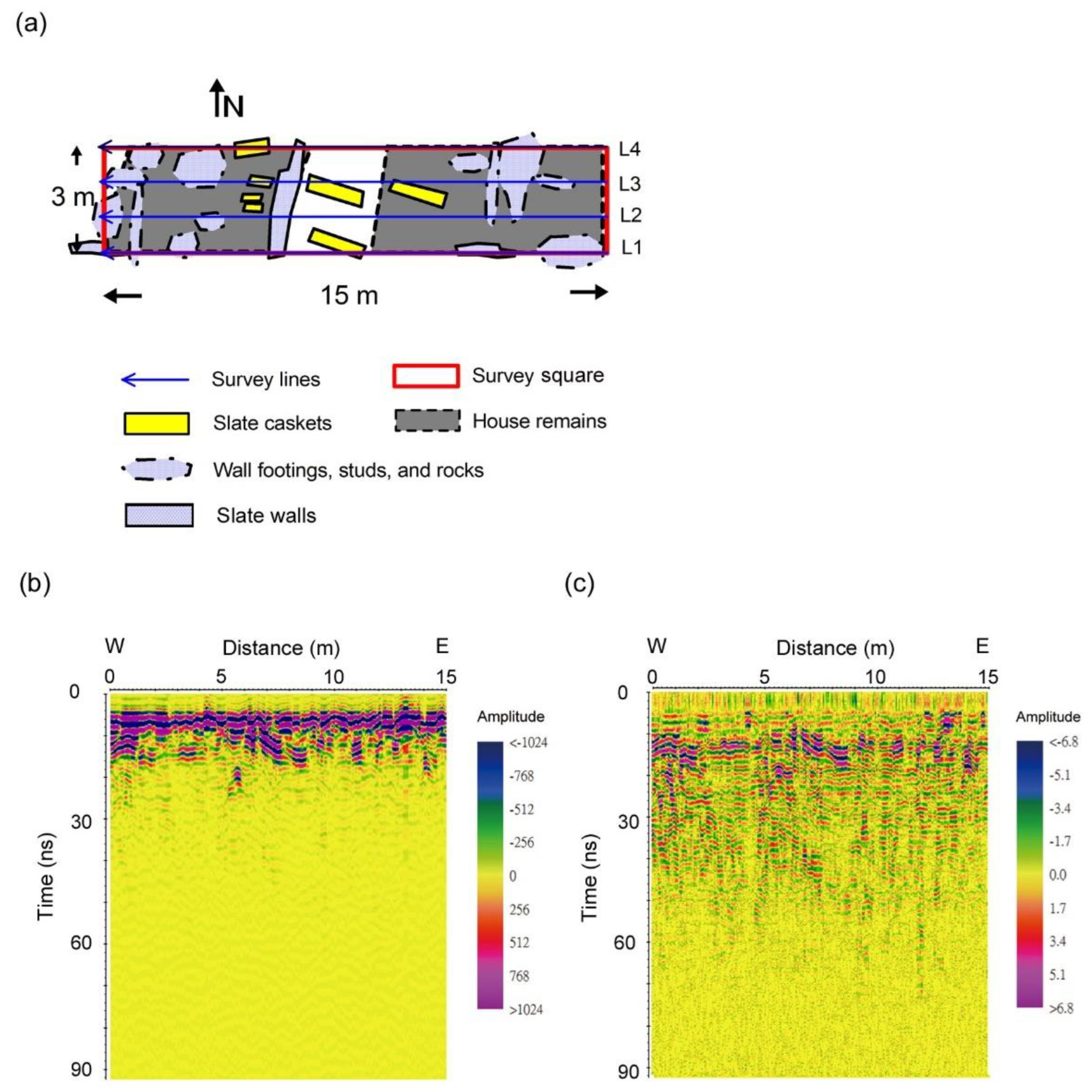
According to the report of Chen [59] and our in-situ positioning, four separate room foundations (Figure 11a) and seven various sizes of caskets (Figure 12a) with a fire pit may exist underneath this square. The structures of these houses are studs and slate walls upheld by cornerstones in a T-shaped feature that constitutes the basis of the house and reinforces the connection between interior and exterior. The remains of the slate walls, studs or pillars, and cornerstones were recovered on the excavation scene and documented. Because of the complexity and interesting objects found in this square, we selected it as a field site for the 3D imaging experiment to assess the effectiveness and limitations of the proposed method. A shielded 500 MHz GPR system was employed to collect the data. We deployed four 15 m survey lines with a line spacing of 1 m at this square (Figure 12a). Each survey line was acquired with the parameters of 0.18 ns temporal sample interval for 512 samples per trace and 0.017 m spatial sample interval on the survey line. The same processing sequence used in the previous model study was applied to each of the survey lines. A typical 2D profile (profile of L1 in Figure 12a) processed using the conventional method is demonstrated in Figure 12b and compared with the result processed using the proposed method (Figure 12c). In conventional processing, background noise removal and a band-pass filter with 100–600 MHz pass-band are applied while data from the same survey line with background noise removal and NLT EEMD were employed to carry out the proposed algorithm fusion. Similar to the control experiment, only one component was selected to reconstruct the data, probably because this site was excavated and then backfilled similarly to the control models.
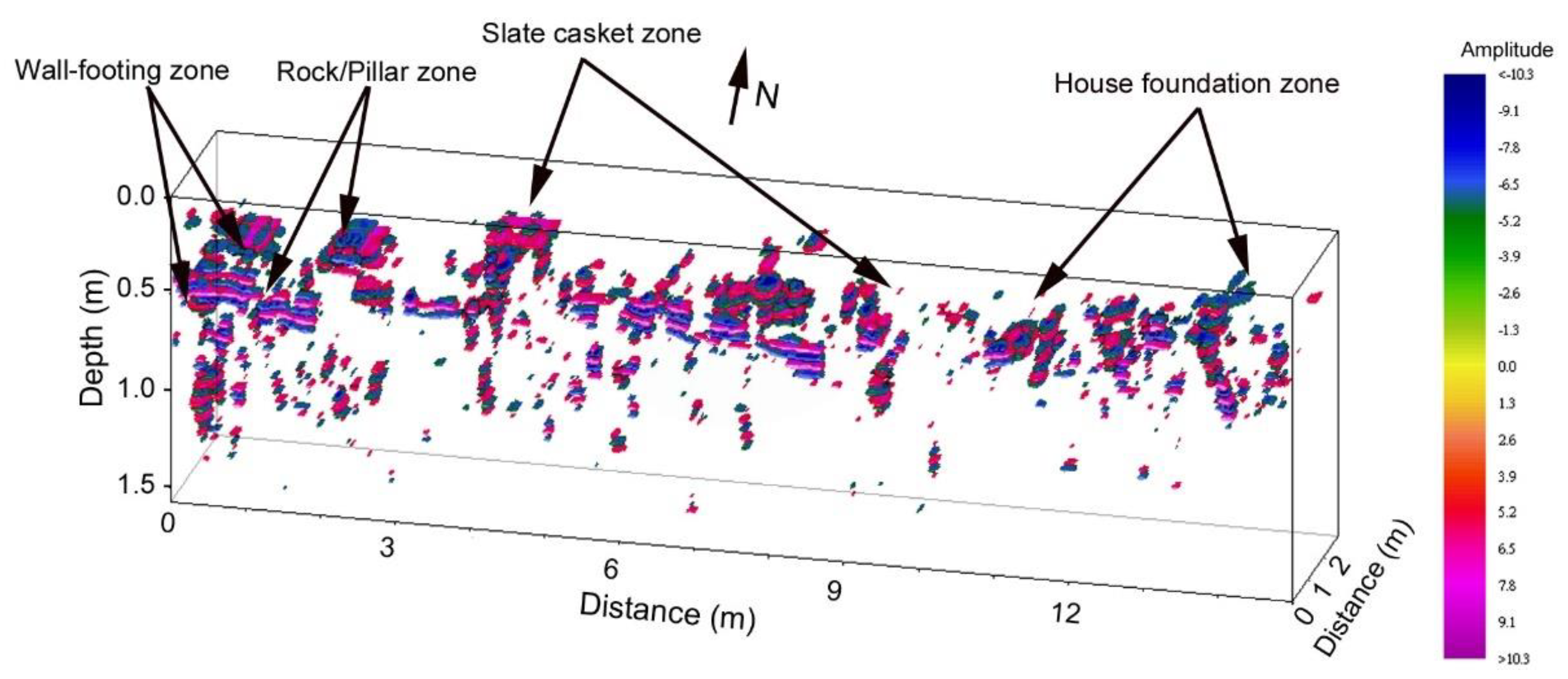
Compared with conventional processing, the coherent horizontal noise in the first 10 ns (Figure 12b) is greatly suppressed using the proposed algorithm fusion, and finer events and deeper reflections are revealed in Figure 12c. Therefore, the proposed method was selected for 3D imaging. However, the difficulty is that the space interval between parallel acquisitions and the lack of transversal scans makes it very hard to expect a reliable 3D interpretation. To achieve the best imaging, we tried to rotate the 3D image based on the potential positions of buried remains indicated on the map (Figure 12a). The result is shown in Figure 13.
The result (Figure 13) indicates that the positions of subsurface features (slate caskets, rocks, wall footings) were generally consistent with the excavation data [59]. Some small caskets and fire pits were not well mapped in Figure 13 because the spatial sample interval (cross-line spacing) did not fulfill full-resolution sampling criteria. More specifically, the maximum spatial sample interval should not exceed ¼ of the apparent wavelength (about 0.04 m in this case) of the GPR signal [29]. Therefore, this survey is spatially aliased in the cross-line direction and should be described as pseudo-3D imaging.

3.2.2. Incomplete Excavation Survey Square

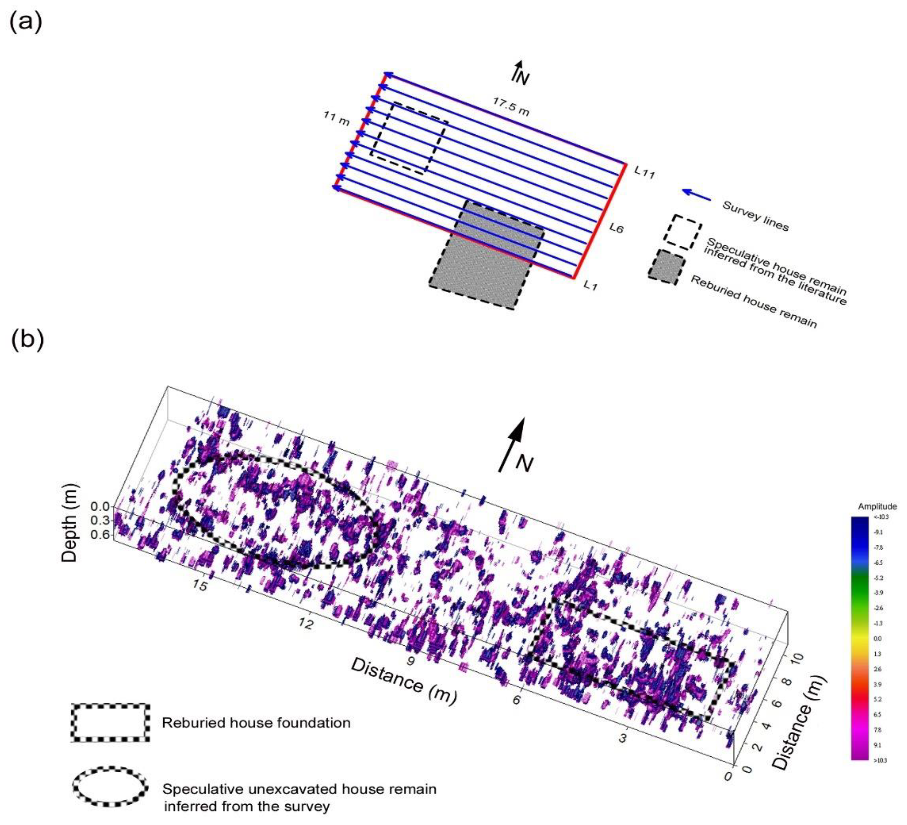
The incomplete excavation survey square is located outside the north fence of the excavated Chuping archaeological site. This area is a cherry orchard at present (Figure 11c). Referring to the Chuping archaeological site map and our on-site landscape survey, Figure 14a indicates that some reburied excavated house remains and a speculative unexcavated house foundation may exist in this square. According to the pictures taken at the time of excavation [59], the floor of this reburied house was paved with small slate fragments (from approximately 4 cm to 30 cm in diameter); therefore, it is an ideal indication for data correlation and interpretation. We targeted this area to find the undiscovered remains and if possible, image a multilayered internal structure of the Chuping archaeological site.
The field data were acquired by deploying eleven survey lines with 1 m line spacing. The line length was about 17.5 m, the temporal sample interval was 0.052 ns for 1024 samples per trace, and the spatial sample interval on the survey line was 0.017 m. One concern for data quality is the interference of vegetation (Figure 11c); it not only hinders the field survey but also may generate pitfall events in data interpretation.
To provide an objective presentation, we still chose the first survey line (L1) in the incomplete excavation survey square as an example. Figure 14b shows the 2D profile of L1 (Figure 14a) processed using the conventional method, and the result of applying the NLT EEMD method is demonstrated in Figure 14c. The pass-band of the linear filter used in the conventional method was determined by referring to the marginal spectrum [6,21,45,49,62] of the selected component. The bandwidth of a 500 MHz center frequency GPR system is between 250 MHz and 750 MHz. We applied the 400–1000 MHz band-pass filter in conventional processing to enhance ultra-shallow targets at the Chuping archaeological site (less than 0.5 m).
Because this square was only excavated in a small area, we aimed to provide an unbiased assessment for a complete deeper, and broader excavation. Considering this point, we eliminated FFTI in the processing sequence to minimize aliasing and artifacts. A pseudo-3D cube constructed by integrating the NLT EEMD processed 2D profiles without interpolation is shown in Figure 15. The dense distribution of spotty events on the southeast side should be the reflections of slate fragments from the excavated house floor, as stated previously. With reasonable inference, the same reflection pattern found on the west side could be an unexcavated house foundation, as expected. Although interpretation could vary, we may conclude that more remains are highly likely to be found in this area.

4. Discussion

All required Matlab code related to EMD, EEMD, and other advanced algorithms is available on the inventors’ websites. For the conventional methods, the algorithms and source code are accessible in the literature and some popular commercial software. Usually, investigators prefer to write their code because it is more flexible in dealing with cases of various fusion conditions. However, an argument may arise that neither the conventional nor the newer nonlinear algorithms within the proposed algorithm fusion scheme are frontier techniques. In that context, there are many major differences in how to handle the research issue. From a practical point of view, the techniques in our algorithm fusion are robust, easy to apply, and most importantly, have low computation costs. These advantages should be encouraging. It is also worth noting that a GPR profile is an assembly of single traces representing cumulative reflections over the recording time. Since the original GPR traces acquired in the field are one-dimensional, it may not be practical to employ multidimensional EEMD [39,41] filtering techniques. In light of our previous research [6,41,45,49,55,62] and personal experiences, we performed a technical survey and compared the test results of the advanced multidimensional EEMD technique and the proposed methodology before carrying out this research. The algorithm fusion technique had a much lower computational cost with an acceptable outcome. Applying a multidimensional algorithm to process data from a 1D feature may only achieve marginal improvements with substantial extra endeavors, and at worst, may generate unexpected artifacts.
The NLT EEMD is the highlight of the proposed algorithm fusion. There are several advanced or alternative EMD algorithms available nowadays. They put forward more considerations and diversify the applications of EMD. One remarkable achievement is Holo–Hilbert spectral analysis, which can precisely determine the linearity and non-linearity of the data to be analyzed, and yields a full spectral representation for nonlinear and non-stationary data in both amplitude and frequency modulation modes [42]. This novel method has been successfully applied to 1D data series with acceptable computing efficiency, and it is possible to process GPR data. However, the complexity of the algorithm and the computation cost for the volume of GPR data could be challenging. In any case, this progress on an EMD algorithm is inspiring and should be a future research topic in GPR data processing.
From the examples presented, it can be seen that interpolation has a significant impact on constructing a 3D GPR dataset, particularly between parallel profiles. We used FFTI to increase sampling density. The advantages are that this method generates stable approximation and enhances the signal of poorly sampled data, but the downsides are that it may still have problems producing aliasing events and unrealistic values if the data sampling density is too low for 3D data construction. However, some improvements are possible if more 2D survey lines traverse the subsurface targets. Another concern when using FFTI is the end effect (data drift or disturbance at the window boundaries when performing transformation). Thus, preserving the original file coordinates, making the end slope more uniformly distributed, and improving the disturbance of the end part are necessary. Admittedly, a more convincing interpolation technique such as shape-preserving spline interpolation [48], which has been successfully applied to improve the EMD algorithm, may alleviate the risk.

5. Conclusions

The proposed algorithm fusion scheme provides several advantages and renders important contributions to GPR field investigation such as minimizing disturbance at the study relic site, reducing labor in the field, providing high-resolution subsurface images, and improving post-processing flexibility.
Since we adopted the interpolation technique for 3D imaging, it could be categorized as pseudo-3D GPR imaging. Due to different techniques performed in data acquisition, seismologists seldom admit GPR 3D surveys to be genuine 3D. They call it 2.5D or pseudo-3D at most because without swath shooting in the field and adequate 3D migration in post-processing, all 3D images may be problematic. What we can do is use the limited resources and support to present a better result. However, with the experimental results and field examples presented, we may conclude that the proposed methodology is useful in increasing the accuracy of a 3D GPR image, particularly in areas where real 3D surveys are difficult to employ, as we experienced at the incomplete excavation survey area. Although it is unlikely that the pseudo-3D method we demonstrated in this study will replace real 3D techniques, the simple processing sequence and relatively straightforward algorithm make it possible to be welcomed by investigators not specializing in geophysics. Nevertheless, when considering preservation and environmental issues for conducting a GPR investigation, the proposed method is a feasible and environmentally friendly option. Extended excavation at the Chuping archaeological site may not be possible at this stage; however, detailed GPR mapping to reveal the unexcavated remains in the subsurface of the Chuping area is still valuable for archaeologists to reconstruct the entire prehistoric settlement of this unique highland relic in Taiwan. We believe that the stated mapping could be obtained with reasonable labor by employing the proposed method. In addition to detecting undiscovered relics, this method is a cost-effective tool for precisely locating spots for re-excavating a backfilled archaeological site if a routine assessment of the advantages of backfilling in preserving cultural heritage is required. We believe that the proposed method is ready for upgrading to real 3D investigation if dense cross-line data are acquired. Although this study presents the advantages of the proposed algorithm, we never disregard conventional methods. As it is said, “no method is perfect”. The proposed method is just an alternative. We hope that some investigators may be interested in this topic and improve it.

Author Contributions

Conceptualization, Y.J.; methodology, Y.J. and H.-M.Y.; software, C.-S.C.; validation, Y.J., H.-M.Y. and C.-S.C.; formal analysis, Y.J., H.-M.Y. and C.-S.C.; investigation, Y.J., H.-M.Y. and C.-S.C.; resources, Y.J.; data curation, H.-M.Y. and C.-S.C.; writing—original draft preparation, Y.J.; writing—review and editing, Y.J.; visualization, Y.J.; supervision, Y.J.; project administration, Y.J.; funding acquisition, Y.J. All authors have read and agreed to the published version of the manuscript.

Funding

This research was partially funded by the National Science Council of Taiwan, ROC, Grant No. NSC 100-2116-M-003-005.

Institutional Review Board Statement

Not applicable.

Informed Consent Statement

Not applicable.

Data Availability Statement

No new data were created.

Acknowledgments

We are grateful to Chung-Yu Chen of the Academia Sinica, Taipei, Taiwan, ROC for kindly providing the Chuping archaeological site documents and field survey suggestions.

Conflicts of Interest

The authors declare no conflict of interest. The funders had no role in the design of the study; in the collection, analyses, or interpretation of data; in the writing of the manuscript; or in the decision to publish the results.

Appendix A

Appendix A.1. EMD and EEMD Methods

EMD is an adaptive, nonlinear data-driven processing method proposed by Huang et al. [21]. This method assumes that signals arise from local oscillations, and any signal can be decomposed into a set of mono-components called intrinsic mode functions (IMFs) and a residue. IMFs satisfy two conditions, as described in Section 2.2 of this paper. In contrast to Fourier transformation, which decomposes a signal into a sum of mono-frequency, constant-amplitude harmonics, IMFs are amplitude/frequency-modulated oscillations that give the embedded non-stationary and nonlinear characteristics of the signal. To decompose a signal into IMFs, a working technique called “sifting” is operated to remove unwanted fluctuations and riding waves. This technique can be summarized as follows:
(a)
Determine the upper and lower envelopes encompassing all data y(t) using a cubic spline.
(b)
Calculate the mean m1(t) of the two envelopes.
(c)
Subtract the mean m1(t) from the data y(t) to obtain the first component h1(t), which is the prototype of IMF C1.
(d)
Test whether h1(t) is an IMF or not. If it is not, h1(t) is treated as the data, and then steps (a) to (c) must be repeated.
(e)
Repeat the sifting procedure j times until the obtained h1j(t) satisfies the conditions of an IMF.
A criterion for the sifting process to stop is carrying out the Cauchy type of convergence test, which guarantees that enough physical sense is retained in the IMF components. The convergence test is performed by calculating the size of the standard deviation, SD, computed from two consecutive sifting results. For a given data set with S + 1 samples, the size of the standard deviation after j times of sifting, SDj, is
S D j = t = 0 S | d j 1 ( t ) d j ( t ) | 2 t = 0 S d j 1 2 ( t )
where dj is the difference between the input data and the mean of the two envelopes at j times of sifting. Suggested values of SDj are between 0.2 and 0.3 [21]; however, this is an empirical criterion, and a rigorous justification is needed.
When h1j(t) satisfies the conditions of an IMF, it is designated as IMF c1, indicating the first IMF decomposed from the data. Component c1 can then be separated from the rest of the data by subtracting it from the original data, and a residue r1 results. The residue may contain lower frequency components and is treated as the new data for generating the next level’s IMF. The decomposition process is stopped when the residue rn is less than a predetermined stoppage value, or the residue becomes a monotonic function from which no more IMF can be extracted. Consequently, the original data set is iteratively decomposed into a set of IMFs and a residue as
y ( t ) = i = 1 n c i + r n
where ci, i = 1, …, n, are the n IMF components of the different frequency bands, and rn is the residue after repeating the sifting procedure n times.
A frequently encountered difficulty in EMD is mode mixing (i.e., signals of different scales are mixed in a single IMF or a signal of the same scale residing in different IMF components). Mode mixing may cause decomposition to be unstable and lack physical uniqueness when applying EMD. In addition, mode mixing is particularly serious when the data are attenuated or contain intermittent signals, and it can disturb the physical meaning and uniqueness of an IMF [6]. Wu and Huang [34] proposed a new noise-assisted data analysis method, EEMD, to overcome the mode mixing problem. EEMD derives each IMF component from the mean of an ensemble of the same level of IMFs, and each IMF in the ensemble consists of the signal plus white noise of finite amplitude. The EEMD algorithm contains steps as follows:
(a)
add a white noise series w(t) of finite amplitude to the original data y(t); then, the noise-added dataset Y(t) is
Y ( t ) = y ( t ) + w ( t ) × R
where R is the ratio of the standard deviation of the added noise amplitude to that of the data y(t).
(b)
Decompose the white noise-added data into IMFs.
(c)
Repeat step (a) and step (b) k times with different white noise series of the same amplitude each time.
(d)
Obtain the (ensemble) means of the corresponding IMFs of the decompositions as
c ¯ j ( t ) = E j ( t ) k = 1 k l = 1 k c j l
where
E j ( t ) = l = 1 k c j l
represents the ensemble of the jth level of IMF.
Because different white noise series do not correlate with one another, they cancel each other out when taking the ensemble mean. Only the signal remains if k (the number of ensemble members) is infinitive. The added white noise series, therefore, provide uniform reference scales in the time-frequency domain for the signal but cause no interference. This approach effectively reduces mode mixing and is a substantial improvement over the EMD method.

References

  1. Davis, J.L.; Annan, A.P. Ground-penetrating radar for high resolution mapping of soil and rock stratigraphy. Geophys. Prospect. 1989, 3, 531–551. [Google Scholar] [CrossRef]
  2. López, Y.Á.; García-Fernández, M. Editorial for the Special Issue “Advanced Techniques for Ground Penetrating Radar Imaging”. Remote Sens. 2021, 13, 3696. [Google Scholar] [CrossRef]
  3. Elseicy, A.; Alonso-Díaz, A.; Solla, M.; Rasol, M.; Santos-Assunçao, S. Combined Use of GPR and Other NDTs for Road Pavement Assessment: An Overview. Remote Sens. 2022, 14, 4336. [Google Scholar] [CrossRef]
  4. Jaw, S.W.; Hashim, M. Squareal accuracy of underground utility mapping using ground penetrating radar. Tunn. Undergr. Space Technol. 2013, 35, 20–29. [Google Scholar] [CrossRef]
  5. Lai, W.W.L.; Dérobert, X.; Annan, P. A review of Ground Penetrating Radar application in civil engineering: A 30-year journey from Locating and Testing to Imaging and Diagnosis. NDT E Int. 2018, 96, 58–78. [Google Scholar]
  6. Chen, C.S.; Jeng, Y. GPR investigation of the near-surface geology in a geothermal river valley using contemporary data decomposition techniques with forward simulation modeling. Geothermics 2016, 64, 439–454. [Google Scholar] [CrossRef]
  7. Guangyou, F.; Pipan, M. Synthetic and field examples of ground-penetrating radar (GPR) profile improvement using two-phase detection techniques. Geophysics 2003, 68, 554–558. [Google Scholar] [CrossRef]
  8. Jeng, Y.; Lin, C.H.; Li, Y.W.; Chen, C.S.; Yu, H.M. Application of sub-image multiresolution analysis of ground-penetrating radar data in a study of shallow structures. J. Appl. Geophys. 2011, 73, 251–260. [Google Scholar] [CrossRef]
  9. Tzanis, A. A versatile tuneable curvelet-like directional filter with application to fracture detection in two-dimensional GPR data. Signal Process. 2017, 132, 243–260. [Google Scholar] [CrossRef]
  10. Oliveira, R.J.; Caldeira, B.; Teixidó, T.; Borges, J.F. GPR Clutter Reflection Noise-Filtering through Singular Value Decomposition in the Bidimensional Spectral Domain. Remote Sens. 2021, 13, 2005. [Google Scholar] [CrossRef]
  11. Miao, X.; Cheadle, S.P. Noise attenuation with wavelet transforms. In SEG Expanded Abstract; Soc. Expl. Geophys.: Tulsa, OK, USA, 1998; pp. 1072–1075. [Google Scholar]
  12. Stollnitz, E.J.; DeRose, T.D.; Salesin, D.H. Wavelets for computer graphics: A primer, Part 1. IEEE Comput. Graph. Appl. 1995, 15, 76–84. [Google Scholar] [CrossRef]
  13. Baåth, M. Spectral Analysis in Geophysics, 1st ed.; Elsevier Science: Amsterdam, The Netherlands, 1974; pp. 25–27. [Google Scholar]
  14. Virieux, J.; Operto, S. An overview of full-waveform inversion in exploration geophysics. Geophysics 2009, 74, WCC1–WCC26. [Google Scholar] [CrossRef]
  15. Jazayeri, S.; Klotzsche, A.; Kruse, S. Improving estimates of buried pipe diameter and infilling material from ground-penetrating radar profiles with full-waveform inversion. Geophysics 2018, 83, H27–H41. [Google Scholar] [CrossRef]
  16. Kruk, J.; Liu, T.; Mozaffari, A.; Gueting, N.; Klotzsche, A.; Vereecken, H.; Warren, C.; Giannopoulos, A. GPR full-waveform inversion, recent developments, and future opportunities. In Proceedings of the 2018 17th International Conference on Ground Penetrating Radar (GPR), Rapperswil, Switzerland, 18–21 June 2018; pp. 1–6. [Google Scholar] [CrossRef]
  17. Asadi, P.; Gindy, M.; Alvarez, M. A machine learning based approach for automatic rebar detection and quantification of deterioration in concrete bridge deck ground-penetrating radar B-scan images. KSCE J. Civ. Eng. 2019, 23, 2618–2627. [Google Scholar] [CrossRef]
  18. Liang, H.; Xing, L.; Lin, J. Application and algorithm of ground-penetrating radar for plant root detection: A review. Sensors 2020, 20, 2836. [Google Scholar] [CrossRef] [PubMed]
  19. Rasol, M.; Pais, J.C.; Perez-Gracia, V.; Solla, M.; Fernandes, F.M.; Fontul, S.; Ayala-Cabrera, D.; Schmidt, F.; Assadollahi, H. GPR monitoring for road transport infrastructure: A systematic review and machine learning insights. Constr. Build. Mater. 2022, 324, 126686. [Google Scholar] [CrossRef]
  20. Priestley, M.B. Evolutionary spectra and non-stationary processes. J. R. Statist. Soc. 1965, B27, 204–237. [Google Scholar] [CrossRef]
  21. Huang, N.E.; Shen, Z.; Long, S.R.; Wu, M.C.; Shih, H.H.; Zheng, Q.; Yen, N.C.; Tung, C.C.; Liu, H.H. The empirical mode decomposition and the Hubert spectrum for nonlinear and non-stationary time series analysis. Proc. R. Soc. A Math. Phys. Eng. Sci. 1998, 454, 903–995. [Google Scholar] [CrossRef]
  22. Kantz, H.; Schreiber, T. Basic topics. In Nonlinear Time Series Analysis; Cambridge University Press: Cambridge, UK, 2003; pp. 1–2. [Google Scholar]
  23. Windrows, B.; Stearns, S.D. Adaptive Signal Processing; Prentice Hall: Englewood Cliffs, NJ, USA, 1985; pp. 3–15. [Google Scholar]
  24. Mandic, D.P.; Rehman, N.; Wu, Z.; Huang, N.E. Empirical mode decomposition based time-frequency analysis of multivariate signals: The power of adaptive data analysis. IEEE Signal Process. Mag. 2013, 30, 74–86. [Google Scholar] [CrossRef]
  25. Huang, N.E.; Wu, Z. A review on Hilbert-Huang Transform: Method and its applications. Rev. Geophys. 2008, 46, 1–23. [Google Scholar] [CrossRef]
  26. Huang, N.E. Hilbert-Huang Transform and Its Applications; World Scientific: Singapore, 2014; pp. 1–26. [Google Scholar]
  27. Neal, A. Ground-penetrating radar and its use in sedimentology: Principles, problems and progress. Earth Sci. Rev. 2004, 66, 261–330. [Google Scholar] [CrossRef]
  28. Grasmueck, M. 3D ground-penetrating radar applied to fracture imaging in gneiss. Geophysics 1996, 61, 1050–1064. [Google Scholar] [CrossRef]
  29. Grasmueck, M.; Weger, R.; Horstmeyer, H. Full-resolution GPR imaging. Geophysics 2005, 70, K12–K19. [Google Scholar] [CrossRef]
  30. Nuzzo, L.; Leucci, G.; Negri, S.; Carrozzo, M.T.; Quarta, T. Application of 3D visualization techniques in the analysis of GPR data for archaeology. Ann. Geophys. 2002, 45, 321–337. [Google Scholar] [CrossRef]
  31. Kelly, T.B.; Angel, M.N.; O’Connor, D.E.; Huff, C.C.; Morris, L.E.; Wach, G.D. A novel approach to 3D modelling ground-penetrating radar (GPR) data—A case study of a cemetery and applications for criminal investigation. Forensic. Sci. Int. 2021, 325, 1–15. [Google Scholar] [CrossRef]
  32. Yilmaz, O. Seismic Data Processing; Soc. Expl. Geophys.: Tulsa, OK, USA, 1987; pp. 1–526. [Google Scholar]
  33. Lathi, B.P. Modern Digital and Analog Communication Systems, 4th ed.; Oxford University Press: New York, NY, USA, 2010; pp. 1–926. [Google Scholar]
  34. Wu, Z.H.; Huang, N.E. Ensemble empirical mode decomposition: A noise-assisted data analysis method. Adv. Adapt. Data Anal. 2009, 1, 1–41. [Google Scholar] [CrossRef]
  35. Gloerson, P.; Huang, N.E. Comparison of interanual intrinsic modes in hemispheric sea ice covers and others geophysical parameters. IEEE Trans. Geosci. Remote Sens. 2003, 41, 1062–1074. [Google Scholar] [CrossRef]
  36. Flandrin, P.; Rilling, G.; Gonçalvés, P. Empirical mode decomposition as a filter bank. IEEE Signal Process. Lett. 2004, 11, 112–114. [Google Scholar] [CrossRef]
  37. Battista, B.M.; Knapp, C.; McGee, T.; Goebel, V. Application of the empirical mode decomposition and Hilbert-Huang transform to seismic reflection data. Geophysics 2007, 72, H29–H37. [Google Scholar] [CrossRef]
  38. Jeng, Y.; Lin, M.-J.; Chen, C.-S.; Wang, Y.-H. Noise reduction and data recovery for a very low frequency electromagnetic survey using the nonlinear decomposition method. Geophysics 2007, 72, F223–F235. [Google Scholar] [CrossRef]
  39. Wu, Z.H.; Huang, N.E.; Chen, X.Y. The multi-dimensional ensemble empirical mode decomposition method. Adv. Adapt. Data Anal. 2009, 1, 339–372. [Google Scholar] [CrossRef]
  40. Bajaj, V.; Pachori, R.B. Classification of seizure and nonseizure EEG signals using empirical mode decomposition. IEEE Trans. Inf. Technol. Biomed. 2012, 16, 1135–1142. [Google Scholar] [CrossRef] [PubMed]
  41. Chen, C.S.; Jeng, Y. A data-driven multidimensional signal-noise decomposition approach for GPR data processing. Comput. Geosci. 2015, 85, 164–174. [Google Scholar] [CrossRef]
  42. Huang, N.E.; Hu, K.; Yang, A.C.C.; Chang, H.-C.; Jia, D.; Liang, W.-K.; Yeh, J.R.; Kao, C.-L.; Juan, C.-H.; Peng, C.K.; et al. On Holo-Hilbert spectral analysis: A full informational spectral representation for nonlinear and non-stationary data. Philos. Trans. R. Soc. A Math. Phys. Eng. Sci. 2016, A374, 20150206. [Google Scholar] [CrossRef] [PubMed]
  43. Hassan, A.R.; Bhuiyan, M.I.H. Automated identification of sleep states from EEG signals by means of ensemble empirical mode decomposition and random under sampling boosting. Comput. Meth. Programs Biomed. 2017, 140, 201–210. [Google Scholar] [CrossRef]
  44. Smulko, J. Methods of trend removal in electrochemical noise data–Overview. Measurement 2019, 131, 569–581. [Google Scholar]
  45. Chen, C.S.; Chien, T.S.; Lee, P.L.; Jeng, Y.; Yeh, T.K. Prefrontal brain electrical activity and cognitive load analysis using a non-linear and non-Stationary approach. IEEE Access 2020, 8, 211115–211124. [Google Scholar] [CrossRef]
  46. Li, M.; Li, Y.B.; Zhang, Q.C.; Shi, Y.T.; Cui, F.P.; Zhao, Y. Research on spark spectrum signal processing based on ensemble empirical mode decomposition. Spectrosc. Spectr. Anal. 2020, 40, 1923–1928. [Google Scholar]
  47. Shaik, M.; Shaik, A.G.; Yadav, S.K. Hilbert-Huang transform and decision tree-based islanding and fault recognition in renewable energy penetrated distribution system. Sustain. Energy Grids Netw. 2022, 30, 100606. [Google Scholar] [CrossRef]
  48. Brown, W.; van der Walt, M. Two-dimensional EMD with Shape-preserving Spline Interpolation. J. Appl. Anal. 2023, in press. [Google Scholar] [CrossRef]
  49. Chen, C.-S.; Jeng, Y. Nonlinear data processing method for the signal enhancement of GPR data. J. Appl. Geophys. 2011, 75, 113–123. [Google Scholar] [CrossRef]
  50. Gonzalez, R.; Woods, R. Digital Image Processing, 2nd ed.; Prentice Hall: Upper Saddle River, NJ, USA, 2002; pp. 76–79. [Google Scholar]
  51. Jiao, Y.; Zhang, F.; Huang, Q.; Liu, X.; Li, L. Analysis of interpolation methods in the validation of backscattering coefficient products. Sensors 2023, 23, 469. [Google Scholar] [CrossRef] [PubMed]
  52. Jeng, Y. Shallow seismic investigation of a site with poor reflection quality. Geophysics 1995, 60, 1715–1726. [Google Scholar] [CrossRef]
  53. Jeng, Y.; Lee, Y.L.; Chen, C.Y.; Lin, M.J. Integrated signal enhancements in magnetic investigation in archaeology. J. Appl. Geophys. 2003, 53, 31–48. [Google Scholar] [CrossRef]
  54. Jeng, Y.; Chen, C.S.; Yu, H.M.; Jeng, A.S.R.; Tang, C.Y.; Lin, M.J. Ultrashallow seismic experiment on a trenched section of the Chelunpu fault zone, Taiwan. Tectonophysics 2007, 443, 255–270. [Google Scholar] [CrossRef]
  55. Chen, C.-S.; Jeng, Y. Multidimensional EMD with marginal Hilbert-Huang spectrum applications for engineering geophysics—Technical tutorial and field example. TLE 2022, 41, 347–356. [Google Scholar] [CrossRef]
  56. Jeng, Y.; Chen, C.S. Subsurface GPR imaging of a potential collapse area in urban environments. Eng. Geol. 2012, 147–148, 57–67. [Google Scholar] [CrossRef]
  57. Booth, A.D.; Linford, N.T.; Clark, R.A.; Murray, T. Three-dimensional, multi-offset ground-penetrating radar imaging of archaeological targets. Archaeol. Prospect. 2008, 15, 93–112. [Google Scholar] [CrossRef]
  58. Böniger, U.; Tronicke, J. Improving the interpretability of 3D GPR data using target-specific attributes: Application to tomb detection. J. Archaeol. Sci. 2010, 37, 672–679. [Google Scholar] [CrossRef]
  59. Chen, C.Y. Chuping-Archaeological Fieldwork Report II; Inst. Hist. Philol. (IHP), Acad. Sin.: Taipei, Taiwan, 1994; pp. 1–479. Available online: https://www1.ihp.sinica.edu.tw/Publications/Book/479 (accessed on 27 January 2023). (In Chinese)
  60. Yu, H.M. Application of Contemporary Time-Frequency Analysis Methods to Pseudo-3D Ground-Penetrating Radar Data. Unpublished. Ph.D. Dissertation, Department of Earth Sciences, National Taiwan Normal University, Taipei, Taiwan, 2012. [Google Scholar]
  61. Yu, H.-M.; Chen, C.-S.; Jeng, Y. Use of ground penetrating radar in studies of the Chuping prehistoric site (In Chinese with English abstract). J. Soc. Reg. Dev. 2012, 3, 67–88. [Google Scholar]
  62. Chen, C.-S.; Jeng, Y. Improving GPR imaging of the buried water utility infrastructure by integrating the multidimensional nonlinear data decomposition technique into the edge detection. Water 2021, 13, 3148. [Google Scholar] [CrossRef]
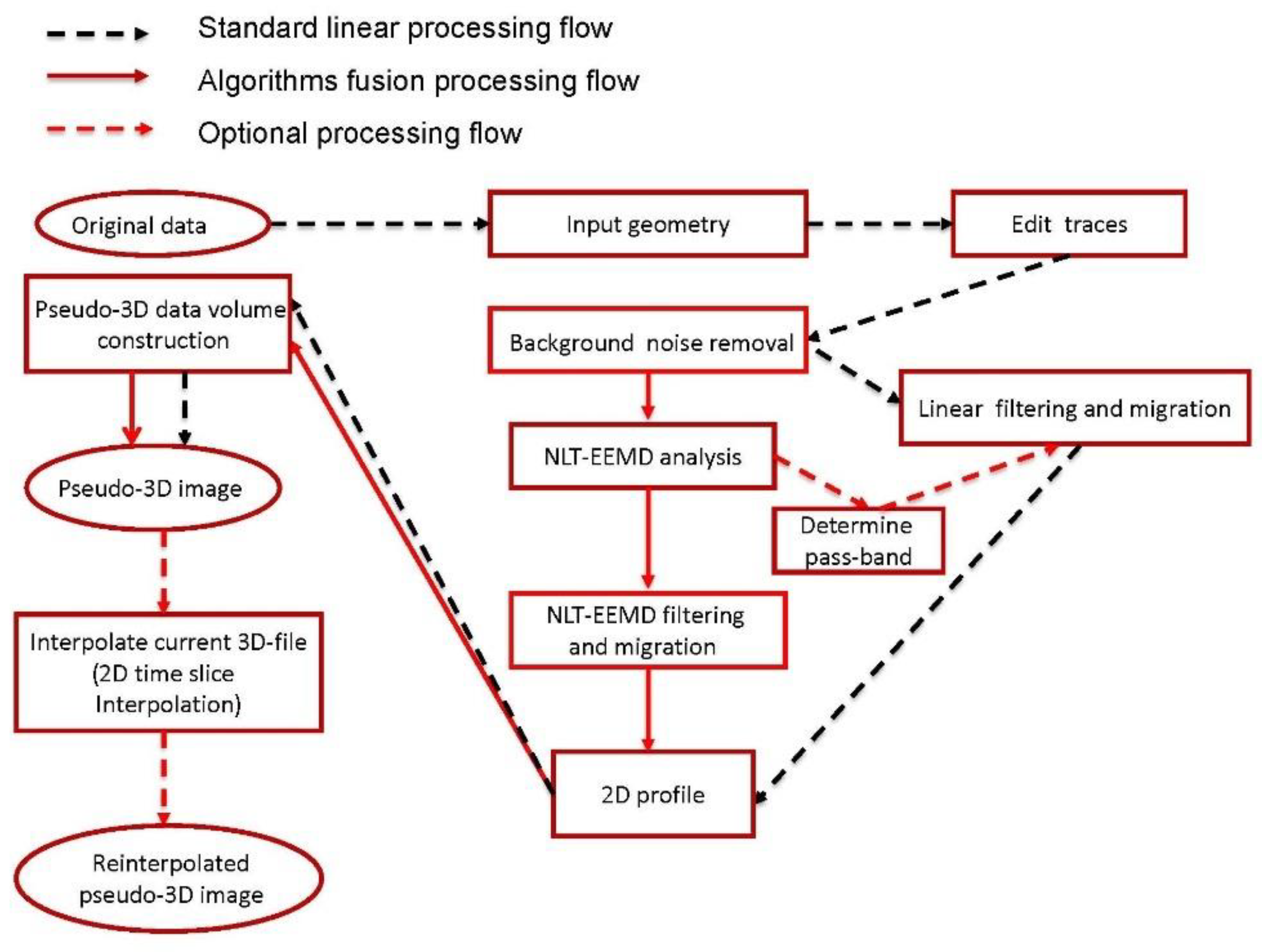
Figure 1. Flowchart of the proposed algorithm fusion. Procedures are the same for the conventional and proposed approach until the completion of background noise removal. After trace editing, the proposed sequence is indicated by the solid red arrow. We use the term pseudo-3D to point out that the original data may not be well-sampled.
Remotesensing 15 02886 g001
Figure 2. Map of Taiwan and landscapes around the Chuping area. The shaded relief map was compiled in Transverse Mercator 2-degree projection (TM2) with a scale in meters.
Remotesensing 15 02886 g002
Figure 3. Brick casket model. (a) Schematic sketch of the buried model. (b) Picture showing survey line EW09 and the projected position of the buried model. (c) Pricking probe survey to confirm the model position.
Remotesensing 15 02886 g003
Figure 4. Linear and NLT processing results for casket model survey line EW09. (a) Original profile in which abnormal pulses and DC bias are removed by the linear method. (b) NLT profile of (a). (c) NLT profile with horizontal background noise removal.
Remotesensing 15 02886 g004
Figure 5. Profile filter bank derived using the EEMD technique. Four significant IMF profile components out of eleven components decomposed from the survey line EW09 profile shown in Figure 4c are demonstrated. (a) Component C3. (b) Component C4. (c) Component C5. (d) Component C6.
Remotesensing 15 02886 g005
Figure 6. Comparison of the proposed scheme with the conventional method. (a) Profile reconstructed using component C4. (b) Profile reconstructed using component C5. Note that in these two subplots, the strong events below the surface reflection are the water table and its multiples (from 5 ns to 10 ns). (c) Profile resulting from the conventional method including background removal, gain function energy compensation, and band-pass filtering. The optimal pass-band of the filter is determined by referring to the spectrograms of the EEMD components.
Remotesensing 15 02886 g006
Figure 7. Miniature model imitating a backfilled house foundation or multilayered objects. The model was two buried DVD drives of different lengths buried at the same site but at different depths. The grid map shows the layout of all survey lines, where the shaded rectangle indicates the position of the buried model.
Remotesensing 15 02886 g007
Figure 8. Original data, NLT data, and EEMD components (C1 to C6) of the GPR profile of E–W survey line T12. The reflection events revealed in the EEMD Component C2 profile clearly indicate two separate reflections from two buried targets. Background noise filtering i = was not applied at this stage. Note that the font of the component number is replaced by a subscript to distinguish it from the symbols used in the 2D algorithm.
Remotesensing 15 02886 g008
Figure 9. Comparison of conventional and EEMD processed 2D images of the miniature model. (a) Conventional profile obtained by using background removal and band-pass filter with pass-band of 400~1000 MHz. (b) Profile reconstructed using NLT EEMD with background removal. The low amplitude values, |amp| ≦ 1024 for conventional processing and |amp| ≦ 7 for NLT EEMD processing, are clipped to enhance the display of the targets. In addition, note that the plotting directions (E–W or W–E) in Figure 8 and Figure 9 are specifically marked to indicate the opposite directions in the figure outputs of the processing software.
Remotesensing 15 02886 g009
Figure 10. Comparison of 3D images of the miniature model. (a) All 21 N–S survey lines were used with conventional filtering methods applied. (b) NLT EEMD processed results using only the three N–S survey lines (L1, L11, and L21) indicated in Figure 7 and interpolating ten equally-spaced lines between two survey lines.
Remotesensing 15 02886 g010
Figure 11. Sketch and pictures showing the field survey squares at the Chuping archaeological site. (a) Sketch of the study area. The background map is redrawn and modified from [59]. In this study, we call the 15 m × 3 m survey square inside the fence the backfilled survey square. The 17.5 m × 11 m survey square outside the north fence is called the incomplete excavation survey square, where another foundation system may exist. The positions of house remains are inferred from the 1980s excavation [59]. (b) Photograph of the fenced backfilled site while conducting the survey. The metallic grid fence shown in this picture is the north boundary of the excavated Chuping archaeological site. (c) Landscape of the incomplete excavation region.
Remotesensing 15 02886 g011
Figure 12. Backfilled survey square and representative 2D profiles. (a) Map with possible buried remains indicated. The house remains may include pieces of slate walls, studs/pillars, cornerstones, and slate rocks. (b) Result of applying standard processing to data from line L1. Background noise removal and band-pass filter with 100–600 MHz pass-band are applied. (c) Result of applying the proposed method. Data from the same survey line with background noise removal and NLT EEMD are applied, and only one component is selected to reconstruct the data.
Remotesensing 15 02886 g012
Figure 13. 3D representation of the interpolated image of the backfilled survey square. The data are processed using the proposed method.
Remotesensing 15 02886 g013
Figure 14. Incomplete excavation survey square and representative 2D profiles. (a) Plan view map of the incomplete excavation survey square (red square), which is located outside the north fence of the Chuping archaeological site. This site may include some reburied excavated house remains and a speculative unexcavated house foundation inferred from the Chuping archaeological site map and our on-site landscape survey. (b) Result of applying standard processing to data from line L1. Background noise removal, band-pass filter with 400–1400 MHz pass-band, and fk migration were applied. The signals of slate fragments are masked by strong coherent horizontal noise. (c) EEMD filtered 2D profile of the same survey line. Background noise removal, NLT EEMD, and fk migration were applied. Similar to the previous cases, only one component was selected to reconstruct the data. More realistic events and deeper structures are imaged as a result.
Remotesensing 15 02886 g014
Figure 15. Pseudo-3D GPR imaging of the incomplete excavation survey square. (a) Plan view map of the survey square. (b) Pseudo-3D GPR imaging of the survey square. Data are processed using the proposed method without interpolation.
Remotesensing 15 02886 g015
Disclaimer/Publisher’s Note: The statements, opinions and data contained in all publications are solely those of the individual author(s) and contributor(s) and not of MDPI and/or the editor(s). MDPI and/or the editor(s) disclaim responsibility for any injury to people or property resulting from any ideas, methods, instructions or products referred to in the content.