Cloud Removal in Remote Sensing Using Sequential-Based Diffusion Models

Abstract

The majority of the optical observations collected via spaceborne optical satellites are corrupted by clouds or haze, restraining further applications of Earth observation; thus, exploring an ideal method for cloud removal is of great concern. In this paper, we propose a novel probabilistic generative model named sequential-based diffusion models (SeqDMs) for the cloud-removal task in a remote sensing domain. The proposed method consists of multi-modal diffusion models (MmDMs) and a sequential-based training and inference strategy (SeqTIS). In particular, MmDMs is a novel diffusion model that reconstructs the reverse process of denosing diffusion probabilistic models (DDPMs) to integrate additional information from auxiliary modalities (e.g., synthetic aperture radar robust to the corruption of clouds) to help the distribution learning of main modality (i.e., optical satellite imagery). In order to consider the information across time, SeqTIS is designed to integrate temporal information across an arbitrary length of both the main modality and auxiliary modality input sequences without retraining the model again. With the help of MmDMs and SeqTIS, SeqDMs have the flexibility to handle an arbitrary length of input sequences, producing significant improvements only with one or two additional input samples and greatly reducing the time cost of model retraining. We evaluate our method on a public real-world dataset SEN12MS-CR-TS for a multi-modal and multi-temporal cloud-removal task. Our extensive experiments and ablation studies demonstrate the superiority of the proposed method on the quality of the reconstructed samples and the flexibility to handle arbitrary length sequences over multiple state-of-the-art cloud removal approaches.

1. Introduction

In recent decades, massive remote sensing data have been collected by Earth-observing satellites, and such data have started to play an important role in a variety of tasks, including environmental monitoring [1], economic development mapping [2], land cover classification [3], and agricultural monitoring [4,5]. However, remote sensing images are often blocked by haze or clouds [6], which impedes the data processing and analysis for target monitoring tasks. Therefore, it is valuable and pivotal to explore the approaches for reconstructing the data corrupted by clouds for subsequent data analysis and employment.

In general, cloud removal can be seen as a special type of inpainting task that fills the missing areas of remote sensing data corrupted by clouds with new and suitable content. Prior approaches to cloud removal can be classified into two main types according to the source of information used for the reconstruction: multi-modal approaches and multi-temporal approaches [7]. In order to expand the information sources, multi-modal approaches [8,9,10,11,12,13,14] have been developed to reconstruct cloud-covered pixels via information translated from synthetic aperture radar (SAR) data or other modal data more robust to the corruption of clouds [15]. Traditional multi-modal approaches [8,9] utilize the digital number of SAR as an indicator to find the repair pixel. Eckardt et al. [9] introduce the term closest feature vector (CFV), combining the closest spectral fit (CSF) algorithm [16] with the synergistic application of multi-spectral satellite images and multi-frequency SAR data. With the wide application of deep learning and the rapid development of generative models, Gao et al. [14] first translate the SAR images into simulated optical images in an object-to-object manner by a specially designed convolutional neural network (CNN) and then fuse the simulated optical images together with the SAR images and the cloudy optical images by a generative adversarial network (GAN) to reconstruct the corrupted area. In contrast to methods using a single time point of observations, multi-temporal approaches [17,18,19,20,21,22] attempt a temporal reconstruction of cloudy observations by means of inference across time series, utilizing the information from other cloud-free time point as a reference, based on the fact that the extent of cloud coverage over a particular region is variable over time and seasons [6]. Traditional multi-temporal approaches [18,19,20] employ hand-crafted filters such as mean and median filters to generate the cloud-covered parts using a large number of images over a specific area. For instance, Ramoino et al. [20] conduct cloud removal using plenty of Sentinel-2 images taken every 6–7 days across a time period of three months. In terms of approaches that utilize deep learning techniques, Sarukkai et al. [17] propose a novel spatiotemporal generator network (STGAN) to better capture correlations across multiple images over an area, leveraging multi-spectral information (i.e., RGB and IR bands of Sentinel-2) to generate a cloud-free image. However, these image reconstruction approaches do not leverage multi-modal information and require a large number of mostly cloud-free images taken over an unchanging landscape, greatly limiting their usability and applications.

Meanwhile, much of the early work on cloud removal used datasets containing simulated cloudy observations, copying cloudy pixel values from one image to another clear-free one [23], but could not precisely reproduce the statistic of satellite images containing natural cloud occurrences [12]. Recently, Ebel et al. [7] curated a new real-world dataset called SEN12MS-CR-TS, which contains both multi-temporal and multi-modal globally distributed satellite observations. They also proposed a sequence-to-point cloud removal method based on 3-D CNN (we denote it as Seq2point) to integrate information across time and within different modalities. However, this method lacks a probabilistic interpretation and the flexibility to handle input sequences of arbitrary length. It just uses the ResNet-based [24] branch and a 3-D CNN structure as a generator to combine the feature maps in the time span and needs to be retrained in a great amount of time when the length of the input sequence changes.

Overall, existing approaches have at least one of three major shortages: (1) They do not use globally distributed real-world datasets, leading to the degraded generalizability of the methods. (2) They are not designed to fully leverage both multi-modal and multi-temporal information to reconstruct the corrupted regions. (3) They lack a probabilistic interpretation and flexibility to handle an arbitrary length of the input sequences.

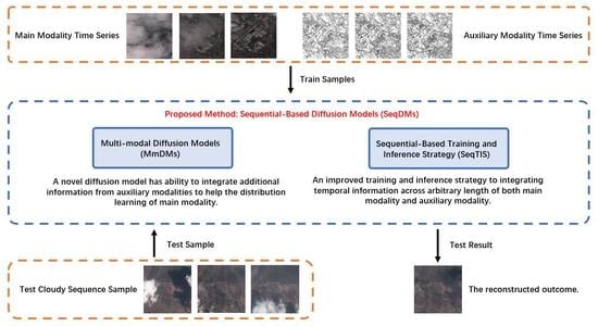
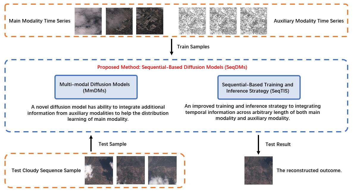
In this paper, we propose a novel method, sequential-based diffusion models (SeqDMs), for the cloud-removal task in remote sensing by integrating information across time and within different modalities. As GANs are known to suffer from the instability training process [25], we choose the denoising diffusion probabilistic models (DDPMs) [26] with a better probabilistic interpretation and a more powerful capability of capturing the data distribution as the backbone model. In particular, we propose novel diffusion models, multi-modal diffusion models (MmDMs), which reconstruct the reverse process of DDPMs to integrate additional information from the auxiliary modalities (e.g., SAR or other modalities robust to the corruption of clouds) to help the distribution learning of main modality (i.e., spaceborne optical satellites data). Since the standard DDPMs training and inference strategy processes the samples only in a single time point, we introduce an improved training and inference strategy named sequential-based training and inference strategy (SeqTIS) to integrate information across time from both main modality and auxiliary modalities input sequences. It is worth noting that SeqDMs have the flexibility to handle an arbitrary length of the input sequences without retraining the model, which significantly reduces the training time cost. We conduct adequate experiments and ablation studies on a globally distributed SEN12MS-CR-TS dataset [7] to evaluate our method and justify its design. We also compare with other state-of-the-art cloud removal approaches to show the superiority of the proposed method.

2. Preliminaries: Denoising Diffusion Probabilistic Models

Our proposed method for cloud removal is based on DDPMs [26]. Here, we first introduce the definition and properties of this type of generative model. The DDPMs define a Markov chain of a diffusion process controlled by a variance schedule ${\{{\beta }_t\in (0,1)\}}_{t=1}^T$ to transform the input sample $x_0$ to white Gaussian noise $x_T\sim \mathcal{N}(0,\mathbf{I})$ in T diffusion time steps. The symbol t represents the diffusion time steps in the diffusion process of DDPMs. We use the symbol l to represent the sample index in sequential data later. In order to distinguish ’time step’ in the diffusion process of the model and in sequential data, we describe it as ’diffusion time step’ and ’sequential time step’, separately. Each step in the diffusion process is given by:

$$q(x_t|x_{t-1})=\mathcal{N}(x_t;\sqrt{1-{\beta }_t}{x}_{t-1},{\beta }_t\mathbf{I}).$$

(1)

The sample $x_t$ is obtained by slowly adding i.i.d. Gaussian random noise with variance ${\beta }_t$ at diffusion time step t and scaling the previous sample $x_{t-1}$ with $\sqrt{1-{\beta }_t}$ according to the variance schedule. A notable property of the diffusion process is that it admits sampling $x_t$ at an arbitrary diffusion time step t from the input $x_0$ in a closed form as

$$q(x_t|x_0)=\mathcal{N}(x_t;\sqrt{{\overline{\alpha }}_t}{x}_0,(1-{\overline{\alpha }}_t)\mathbf{I}),$$

(2)

where ${\alpha }_t:=1-{\beta }_t$ and ${\overline{\alpha }}_t:={\prod }_{s=1}^t{\alpha }_s$.

The inference process (the generation direction) works by sampling a random noise vector $x_T$ and then gradually denoising it until reaches a high-quality output sample $x_0$. To implement the inference process, the DDPMs are trained to reverse the process in Equation (1). The reverse process is modeled by a neural network that predicts the parameters ${\mu }_{\theta }(x_t,t)$ and ${\Sigma }_{\theta }(x_t,t)$ of a Gaussian distribution:

$$p_{\theta }(x_{t-1}|x_t)=\mathcal{N}(x_{t-1}; {\mu }_{\theta }(x_t,t),{\Sigma }_{\theta }(x_t,t)).$$

(3)

The learning objective for the model in Equation (3) is derived by considering the variational lower bound,

$$\mathbb{E}[-log{p}_{\theta }(x_0)]\le {\mathbb{E}}_q[-log\frac{p_{\theta }(x_{0:T})}{q(x_{1:T}|x_0)}]={\mathbb{E}}_q[-logp(x_T)-\sum _{t\ge 1}log\frac{p_{\theta }(x_{t-1}|x_t)}{q(x_t|x_{t-1})}]=L_{VLB},$$

(4)

and this objective function can be further decomposed as:

$$L_{VLB}={\mathbb{E}}_q[\underset{L_T}{\underbrace{D_{KL}(q(x_T|x_0)\left|\right|p(x_T))}}+\sum _{t>1}\underset{L_{t-1}}{\underbrace{D_{KL}(q(x_{t-1}|x_t,x_0)\left|\right|p_{\theta }(x_{t-1}|x_t))}}\underset{L_0}{\underbrace{-log{p}_{\theta }(x_0|x_1)}}].$$

(5)

It is noteworthy that the term $L_{t-1}$ trains the network in Equation (3) to perform one reverse diffusion step. Furthermore, the posterior $q(x_{t-1}|x_t)$ is tractable when conditioned on $x_0$, and it allows for a closed form expression of the objective since $q(x_{t-1}|x_t,x_0)$ is also a Gaussian distribution:

$$q(x_{t-1}|x_t,x_0)=\mathcal{N}(x_{t-1}; {\tilde{\mu }}_t(x_t,x_0),{\tilde{\beta }}_t\mathbf{I}),$$

(6)

where

$${\tilde{\mu }}_t(x_t,x_0)=\frac{\sqrt{{\overline{\alpha }}_{t-1}}{\beta }_t}{1-{\overline{\alpha }}_t}{x}_0+\frac{\sqrt{{\alpha }_t}(1-{\overline{\alpha }}_{t-1})}{1-{\overline{\alpha }}_t}{x}_t$$

(7)

and

$${\tilde{\beta }}_t=\frac{1-{\overline{\alpha }}_{t-1}}{1-{\overline{\alpha }}_t}{\beta }_t.$$

(8)

Instead of directly predicting ${\tilde{\mu }}_t$, a better way is to parametrize the model by predicting the cumulative noise $\epsilon$ that is added to the current intermediate sample $x_t$:

$${\mu }_{\theta }(x_t,t)=\frac{1}{\sqrt{{\alpha }_t}}(x_t-\frac{{\beta }_t}{\sqrt{1-\overline{{\alpha }_t}}}{\epsilon }_{\theta }(x_t,t)),$$

(9)

then, the following simplified training objective is derived from the term $L_{t-1}$ in Equation (5):

$$L_{simple}={\mathbb{E}}_{t,x_0,\epsilon }[{\left|\right|\epsilon -{\epsilon }_{\theta }(\sqrt{{\overline{\alpha }}_t}{x}_0+\sqrt{1-{\overline{\alpha }}_t}\epsilon ,t)\left|\right|}^2].$$

(10)

As introduced by Nichol and Dhariwal [27], learning variance ${\Sigma }_{\theta }(x_t,t)$ in Equation (3) of the reverse process helps to improve the log-likelihood and reduce the number of sampling steps. Since $L_{simple}$ does not depend on ${\Sigma }_{\theta }(x_t,t)$, they define a new hybrid objective:

$$L_{hybrid}=L_{simple}+\lambda L_{VLB}.$$

(11)

Furthermore, they make DDPMs achieve better sample quality than the current state-of-the-art generative models by finding a better architecture through a series of ablations [28]. Hence, we base our proposed method on DDPMs.

3. Materials and Methods

In this section, we describe in detail the proposed method sequential-based diffusion models (SeqDMs) for cloud removal in remote sensing, which consists of two components. In Section 3.1, we first present novel diffusion models, multi-modal diffusion models (MmDMs), which leverage a sequence of auxiliary modal data as additional information to learn the distribution of main modality. In Section 3.2, we introduce an improved training and inference strategy named sequential-based training and inference strategy (SeqTIS) for cloud removal to integrate information across time from both the main modality (i.e., optical satellite data) and auxiliary modalities (e.g., SAR or other modalities more robust to the corruption of clouds) input sequences.

3.1. Multi-Modal Diffusion Models

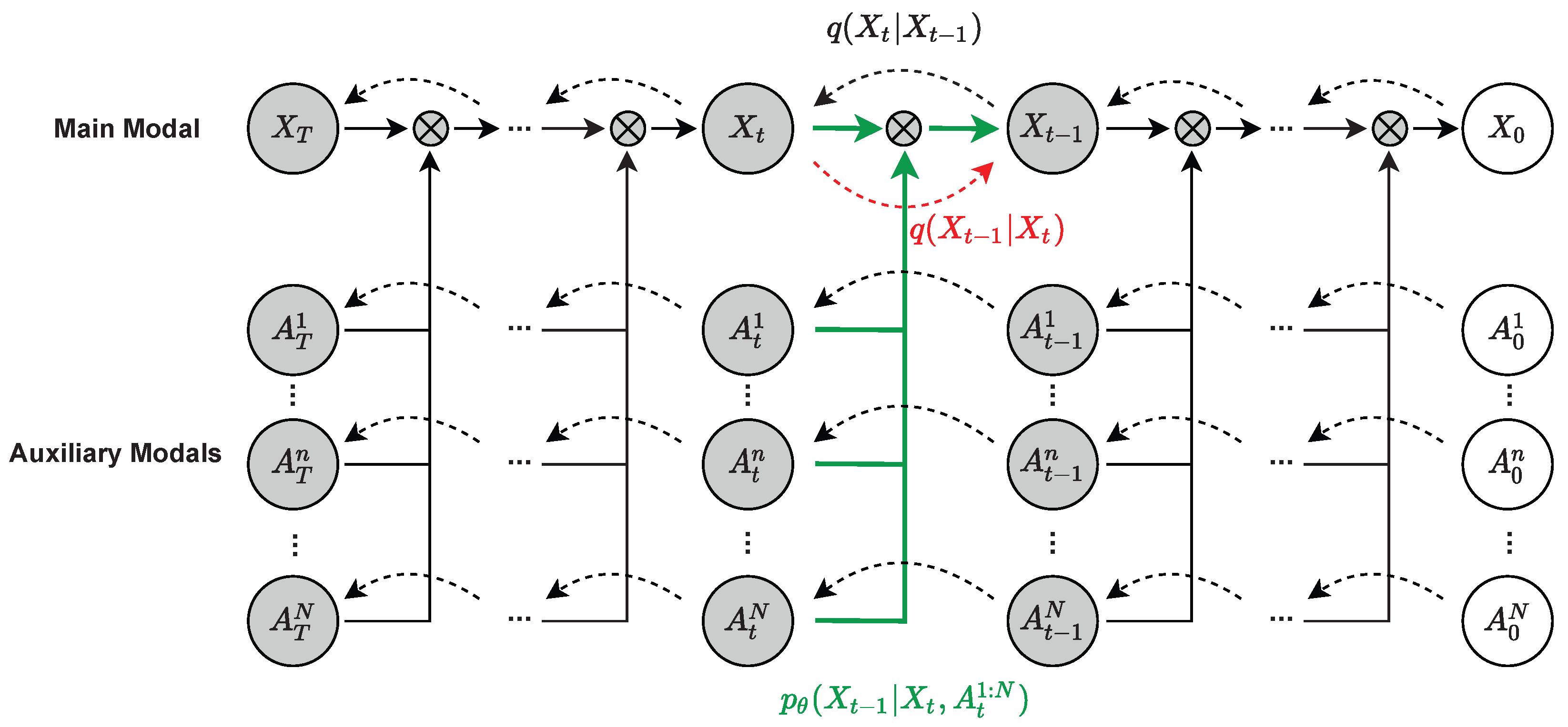
Unlike prior diffusion models [26,27,28], multi-modal diffusion models (MmDMs) leverage auxiliary modalities data as additional inputs to learn the distribution of the main modality, which will complement the partial missing information of the main modality during the inference process (cloud-removal process). The graphical model for MmDMs is shown in Figure 1.

We denote a sequence of multi-modal input data as $\{X,A^1,...,A^n,...,A^N\}$, which consists of one main modality X, as well as N auxiliary modalities A. Since optical satellite data are susceptible to haze or clouds and SAR or other modalities are more robust against these influences [6,15], we consider optical satellite data as the main modality X and SAR or other modalities as auxiliary modalities A in this paper. The most important feature of MmDMs is the powerful ability to capture the distribution of X, and the ability to complement the missing information of X with A during the inference process, leading to a better performance of cloud removal in remote sensing.

The diffusion process of MmDMs is similar to that of DDPMs; it involves individually transforming each modal input sample to white Gaussian noise according to the same variance schedule ${\{{\beta }_t\in (0,1)\}}_{t=1}^T$ in T diffusion time steps. Each diffusion step of the main-modality sample $X_0$ is given by:

$$q(X_{1:T}|X_0):=\prod _{t=1}^{T}q(X_t|X_{t-1}),q(X_t|X_{t-1})=\mathcal{N}(X_t;\sqrt{1-{\beta }_t}{X}_{t-1},{\beta }_t\mathbf{I}),$$

(12)

and the diffusion step for the nth auxiliary modal sample $A_0^n$ is given by:

$$q(A_{1:T}^n|A_0^n):=\prod _{t=1}^{T}q(A_t^n|A_{t-1}^n),q(A_t^n|A_{t-1}^n)=\mathcal{N}(A_t^n;\sqrt{1-{\beta }_t}{A}_{t-1}^n,{\beta }_t\mathbf{I}).$$

(13)

Instead of directly learning a neural network $p_{\theta }(X_{t-1}|X_t)$ to approximate the intractable posterior distribution $q(X_{t-1}|X_t)$ described in Equation (5) of DDPMs, MmDMs add the auxiliary modalities as conditions to the reverse process:

$$p_{\theta }(X_{0:T}|A_{1:T}^{1:N}):=p(X_T)\prod _{t=1}^T{p}_{\theta }(X_{t-1}|X_t,A_t^{1:N}),$$

(14)

$$p_{\theta }(X_{t-1}|X_t,A_t^{1:N})=\mathcal{N}(X_{t-1}; {\mu }_{\theta }(X_t,A_t^{1:N},t),{\Sigma }_{\theta }(X_t,A_t^{1:N},t)).$$

(15)

Then, the training objective for the model in Equation (15) is derived by the variational lower bound on negative log likelihood:

$$\mathbb{E}[-log{p}_{\theta }(X_0)]\le {\mathbb{E}}_q[-log\frac{p_{\theta }(X_{0:T}|A_{1:T}^{1:N})}{q(X_{1:T}|X_0)}]={\mathbb{E}}_q[-logp(X_T)-\sum _{t\ge 1}log\frac{p_{\theta }(X_{t-1}|X_t,A_t^{1:N})}{q(X_t|X_{t-1})}]=L_{VLB},$$

(16)

and it can be further rewritten as:

$$L_{VLB}={\mathbb{E}}_q[\underset{L_T}{\underbrace{D_{KL}(q(X_T|X_0)\left|\right|p(X_T))}}+\sum _{t>1}\underset{L_{t-1}}{\underbrace{D_{KL}(q(X_{t-1}|X_t,X_0)\left|\right|p_{\theta }(X_{t-1}|X_t,A_t^{1:N}))}}\underset{L_0}{\underbrace{-log{p}_{\theta }(X_0|X_1,A_1^{1:N})}}].$$

(17)

Based on Equations (6)–(10) and the property of the diffusion process, we can derive a new version of the simplified training objective from the term $L_{t-1}$ in Equation (17):

$$L_{simple}(\theta )={\mathbb{E}}_{t,X_0,{\epsilon }_x,A_0^{1:N},{\epsilon }_a^{1:N}}[{\left|\right|{\epsilon }_x-{\epsilon }_{\theta }(\sqrt{{\overline{\alpha }}_t}{X}_0+\sqrt{1-{\overline{\alpha }}_t}{\epsilon }_x,\sqrt{{\overline{\alpha }}_t}{A}_0^{1:N}+\sqrt{1-{\overline{\alpha }}_t}{\epsilon }_a^{1:N},t)\left|\right|}^2],$$

(18)

where ${\epsilon }_x$ is the cumulative noise added to the main modal sample $X_0$ and ${\epsilon }_a^{1:N}$ are the noises individually added to N auxiliary modal samples $A_0^{1:N}$.

3.2. Sequential-Based Training and Inference Strategy

To better reconstruct the missing information corrupted by clouds or haze, we introduce sequential-based training and inference strategy (SeqTIS) to integrate the information across time from both main modality and auxiliary modalities. SeqTIS contains a temporal training strategy and a conditional inference strategy, both of which use a reusable module called sequential data fusion module. For ease of description, we extend the multi-modal input data $\{X,A^1,...,A^n,...,A^N\}$ in a prior section into a multi-modal and multi-temporal version $\{X^L,A^{1\_L},...,A^{n\_L},...,A^{N\_L}\}$, where $X^L=\{x^1,...,x^l...,x^L\}$ and $A^{n\_L}=\{a^{n\_1},...,a^{n\_l},...,a^{n\_L}\}$ are the time series of length L. Corresponding to the multi-modal and multi-temporal input data, we also have a ground truth sequence $\{\widehat{X},{\widehat{A}}^1,...,{\widehat{A}}^n,...{\widehat{A}}^N\}$, which contains cloud-free main modality $\widehat{X}$. All of the modules and processes in SeqTIS are described below.

3.2.1. Sequential Data Fusion Module

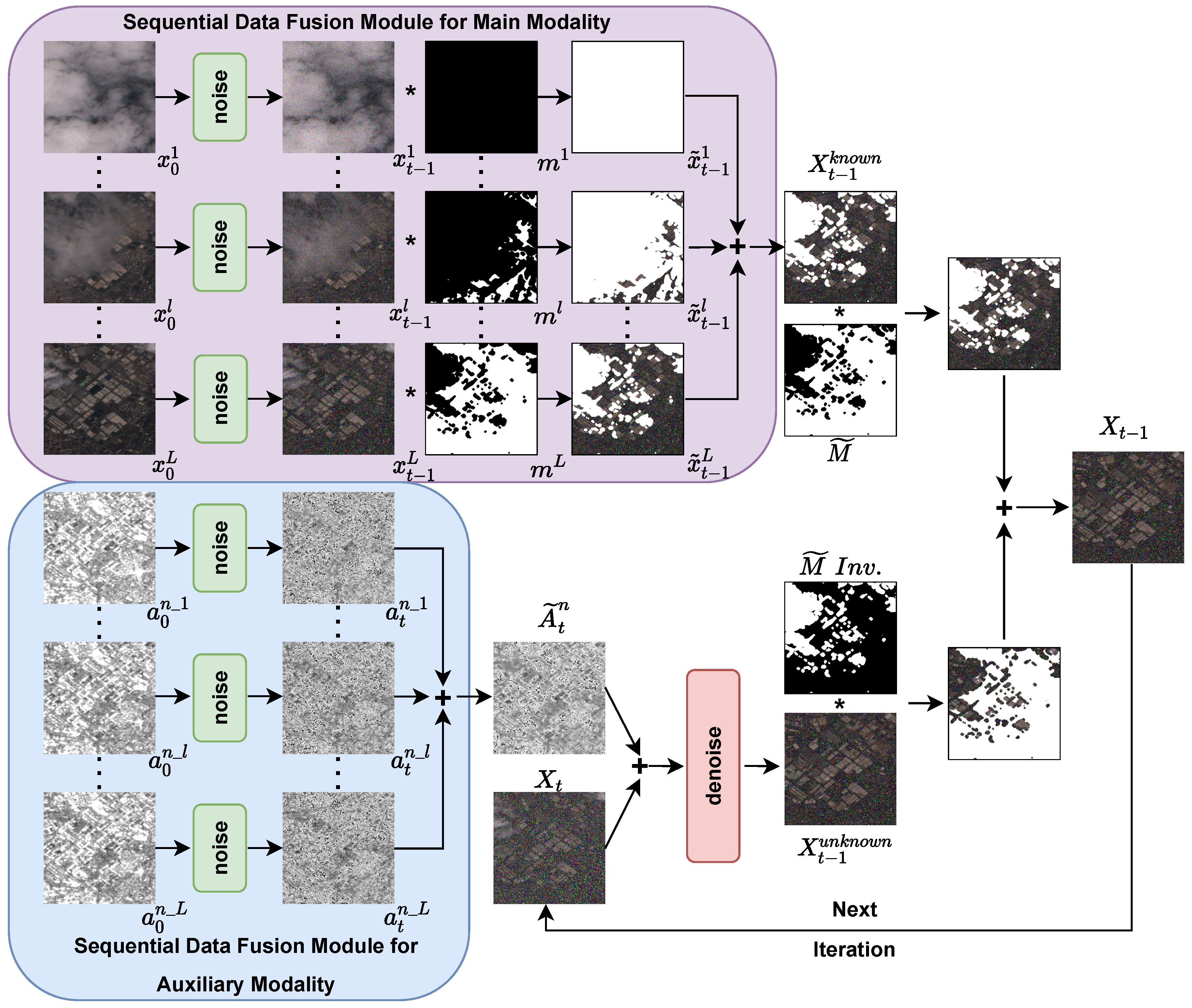
As shown in Figure 2, the sequential data fusion modules are used to integrate the information across time in each modality and are designed separately for either main modality or auxiliary modalities.

Since the auxiliary modalities $A^{1:N}$ are not influenced by clouds or haze, the sequential data fusion module for auxiliary modality is simply designed to individually diffuse data in each sequential time step l into a certain diffusion time step t and then calculate an average weighted value of that diffusion time step to integrate information across time. The nth auxiliary modality sequence $A^{n\_L}$ is processed by the sequential data fusion module for auxiliary modality as follows:

$$a_t^{n\_l}\sim \mathcal{N}(\sqrt{{\overline{\alpha }}_t}{a}_0^{n\_l},(1-{\overline{\alpha }}_t)\mathbf{I})=\sqrt{{\overline{\alpha }}_t}{a}_0^{n\_l}+\sqrt{(1-{\overline{\alpha }}_t)}{\epsilon }_a^{n\_l},l=1,2,...,L,n=1,2,...,N,$$

(19)

where ${\epsilon }_a^{n\_l}\sim \mathcal{N}(0,\mathbf{I})$ is a cumulative noise added to the current intermediate sample $a_t^{n\_l}$. After diffusing the data in each sequential time step l, we calculate the average weighted value of diffusion time step t as follows:

$${\tilde{A}}_t^n=\frac{{\sum }_{l=1}^L{a}_t^{n\_l}}{L},n=1,2,...,N,$$

(20)

which integrates the information of sequence $A^{n\_L}$ across time.

Since the main modality $X^L=\{x^1,...,x^l...,x^L\}$ is susceptible to missing information due to clouds or haze, the sequential data fusion module for the main modality is designed to maintain the known regions’ (cloud-free pixels) information of each sequential time step l as much as possible, which is quite different from that for auxiliary modalities. In order to model the spatial-temporal extent of clouds, the binary cloud masks $M^L=\{m^1,...,m^l...,m^L\}$ are computed on-the-fly for each main modality data in $X^L$ via the cloud detector of s2cloudless [29]. The pixel value 1 of $m^l$ indicates a cloud-free pixel, and value 0 indicates a cloudy pixel. The main modality sequence $X^L$ is processed by the sequential data fusion module for the main modality to the diffusion time step $t-1$ as follows:

$$x_{t-1}^l\sim \mathcal{N}(\sqrt{{\overline{\alpha }}_{t-1}}{x}_0^l,(1-{\overline{\alpha }}_{t-1})\mathbf{I})=\sqrt{{\overline{\alpha }}_{t-1}}{x}_0^l+\sqrt{(1-{\overline{\alpha }}_{t-1})}{\epsilon }_x^l,l=1,2,...,L,$$

(21)

where ${\epsilon }_x^l$ is the noise added to the intermediate sample $x_{t-1}^l$. Then, we maintain the known regions information of $x_{t-1}^l$ by:

$${\tilde{x}}_{t-1}^l=x_{t-1}^l\odot m^l,$$

(22)

where ⊙ indicates the pixel-wise multiplication. Finally, we calculate a weighted value of known regions at diffusion time step $t-1$ for each pixel according to the frequency of value 1, which occurs in masks $M^L$ throughout the whole time step L:

$$X_{t-1}^{known}=\frac{{\sum }_{l=1}^L{\tilde{x}}_{t-1}^l}{{\sum }_{l=1}^L{m}^l+s},$$

(23)

where s is a small offset (set to ${10}^{-19}$) to prevent the unknown regions’ pixels divided by 0.

3.2.2. Conditional Inference Strategy

Before the training strategy, we first describe in detail the conditional inference strategy of SeqTIS, whose overview is shown in Figure 2.

The goal of cloud removal is to reconstruct the pixels corrupted by clouds or haze in optical satellite data using information from known regions (cloud-free pixels) or other modalities as a condition. In order to obtain as many as possible known regions for cloud removal, the multi-modal and multi-temporal sequences $\{X^L,A^{1\_L},...,A^{n\_L},...,A^{N\_L}\}$ are used as inputs to the models during the inference process (cloud-removal process).

Since each reverse step in Equation (15) from $X_t$ to $X_{t-1}$ depends on both the main modality $X_t$ and the auxiliary modalities $A_t^{1:N}$, we need to integrate information across the time of each modality sequence first and then alter the known regions, as long as the correct properties of the corresponding distribution can be maintained.

In order to integrate the information of the main modality $X^L$ at diffusion time step $t-1$, we use the sequential data fusion module for the main modality expressed by Equations (21)–(23) to obtain the known regions’ information $X_{t-1}^{known}$. Then, we use the sequential data fusion modules for auxiliary modality expressed by Equations (19) and (20) to obtain the information integrated value ${\tilde{A}}_t^{1:N}$. After that, we can obtain the unknown regions (corrupted by clouds or haze) information at $t-1$ by using both $X_t$ and ${\tilde{A}}_t^{1:N}$ as inputs:

$$X_{t-1}^{unknown}\sim \mathcal{N}({\mu }_{\theta }(X_t,{\tilde{A}}_t^{1:N},t),{\Sigma }_{\theta }(X_t,{\tilde{A}}_t^{1:N},t))$$

(24)

To utilize the information from the known regions as fully as possible, we define a region mask $\tilde{M}$ for altering the known regions as follows:

$$\tilde{M}=\Theta (\sum _{l=1}^L{m}^l),$$

(25)

where $\Theta$ is a pixel-wise indicator, meaning that the output value will be 1 if the pixel value at the corresponding position is not 0; otherwise, it will be 0. Finally, we can keep the known regions’ information and obtain the next reverse step intermediate $X_{t-1}$ as follows:

$$X_{t-1}=\tilde{M}\odot X_{t-1}^{known}+(1-\tilde{M})\odot X_{t-1}^{unknown}$$

(26)

The conditional inference strategy allows us to integrate temporal information across the arbitrary length of input sequences without retraining the model, which significantly reduces the training cost and increases the flexibility of inference. Algorithm 1 displays the above complete procedure of the conditional inference strategy.

Algorithm 1 Conditional inference (cloud removal) strategy of SeqTIS

1: $X_T\sim \mathcal{N}(0,\mathbf{I})$ 2: for $t=T,...,1$ do 3:     for $l=1,...,L$ do 4:         ${\epsilon }_x^l\sim \mathcal{N}(0,\mathbf{I})$ if $t>1$, else ${\epsilon }_x^l=0$ 5:         $x_{t-1}^l\sim \mathcal{N}(\sqrt{{\overline{\alpha }}_{t-1}}{x}_0^l,(1-{\overline{\alpha }}_{t-1})\mathbf{I})=\sqrt{{\overline{\alpha }}_{t-1}}{x}_0^l+\sqrt{(1-{\overline{\alpha }}_{t-1})}{\epsilon }_x^l$ 6:         ${\tilde{x}}_{t-1}^l=x_{t-1}^l\odot m^l$ 7:         for $n=1,...,N$ do 8:            ${\epsilon }_a^{n\_l}\sim \mathcal{N}(0,\mathbf{I})$ if $t>1$, else ${\epsilon }_a^{n\_l}=0$ 9:            $a_t^{n\_l}\sim \mathcal{N}(\sqrt{{\overline{\alpha }}_t}{a}_0^{n\_l},(1-{\overline{\alpha }}_t)\mathbf{I})=\sqrt{{\overline{\alpha }}_t}{a}_0^{n\_l}+\sqrt{(1-{\overline{\alpha }}_t)}{\epsilon }_a^{n\_l}$ 10:         end for 11:     end for 12:     ${\tilde{A}}_t^n=\frac{{\sum }_{l=1}^L{a}_t^{n\_l}}{L},$ where $n=1,2,...,N$ 13:     $X_{t-1}^{unknown}\sim \mathcal{N}({\mu }_{\theta }(X_t,{\tilde{A}}_t^{1:N},t),{\Sigma }_{\theta }(X_t,{\tilde{A}}_t^{1:N},t))$ 14:     $X_{t-1}^{known}=\frac{{\sum }_{l=1}^L{\tilde{x}}_{t-1}^l}{{\sum }_{l=1}^L{m}^l+s}$ 15:     $\tilde{M}=\Theta ({\sum }_{l=1}^L{m}^l)$ 16:     $X_{t-1}=\tilde{M}\odot X_{t-1}^{known}+(1-\tilde{M})\odot X_{t-1}^{unknown}$ 17: end for 18: return$X_0$

3.2.3. Temporal Training Strategy

Unlike RePaint [30], which only uses the pre-trained unconditional DDPMs based on RGB dataset as a prior, it is necessary to train MmDMs based on multi-spectral satellite data from the beginning. Therefore, we propose a specific training strategy, the temporal training strategy, to accurately capture the real distribution of cloud-free main modality $q(\widehat{X})$ and to force the models to fully leverage the auxiliary modalities’ information to deal with the extreme absence of the main modality.

In order to capture the distribution of $q(\widehat{X})$ as a cloud removal prior, we leverage the powerful distribution capture capability of MmDMs by using the cloud-free samples $\{\widehat{X},{\widehat{A}}^{1:N}\}$ in training split as inputs and optimize the parameter $\theta$ in the neural networks as follows:

$${▿}_{\theta }[{\left|\right|{\epsilon }_{\widehat{x}}-{\epsilon }_{\theta }(\sqrt{{\overline{\alpha }}_t}{\widehat{X}}_0+\sqrt{1-{\overline{\alpha }}_t}{\epsilon }_{\widehat{x}},\sqrt{{\overline{\alpha }}_t}{\widehat{A}}_0^{1:N}+\sqrt{1-{\overline{\alpha }}_t}{\epsilon }_{\widehat{a}}^{1:N},t)\left|\right|}^2+\lambda L_{VLB}].$$

(27)

where ${\epsilon }_{\widehat{x}}\sim \mathcal{N}(0,\mathbf{I})$ is the noise added to the input sample ${\widehat{X}}_0$.

Due to the probability of each sample of cloudy input sequence $X^L$ being severely corrupted by clouds, we have to force the models to make full use of the information from the auxiliary modalities by training with the cloudy sequences as well. We need to process $X^L$ and $A^{(1:N)\_L}$ in the training split by the sequential data fusion modules to obtain the known regions’ information $X_t^{known}$ and ${\tilde{A}}_t^{1:N}$ at diffusion time step t. Then, we use the Gaussian random noise $\mathcal{N}(0,\mathbf{I})$ to fill the unknown regions and optimize the parameter $\theta$ as follows:

$${▿}_{\theta }[{\left|\right|{\epsilon }_{\widehat{x}}-{\epsilon }_{\theta }(X_t,{\tilde{A}}_t^{1:N},t)\left|\right|}^2+\lambda L_{VLB}].$$

(28)

Algorithm 2 displays the complete procedure of the temporal training strategy in detail.

Algorithm 2 Temporal training strategy of SeqTIS

1: repeat 2:     ${\widehat{X}}_0\sim q(\widehat{X})$ 3:     ${\widehat{A}}_0^n,$ where $n=1,2,...,N$          ▹ coregistered and paired with ${\widehat{X}}_0$ 4:     $X_0^L=\{x_0^1,...,x_0^l...,x_0^L\}$               ▹ corresponding to ${\widehat{X}}_0$ 5:     $A_0^{(1:N)\_L}=\{a_0^{(1:N)\_1},...,a_0^{(1:N)\_l},...,a_0^{(1:N)\_L}\}$     ▹ coregistered and paired with $X_0^L$ 6:     $t\sim$ Uniform $(\{1,...,T\})$ 7:     ${\epsilon }_{\widehat{x}}\sim \mathcal{N}(0,\mathbf{I})$ if $t>1$, else ${\epsilon }_{\widehat{x}}=0$ 8:     ${\epsilon }_{\widehat{a}}^n\sim \mathcal{N}(0,\mathbf{I})$ if $t>1$, else ${\epsilon }_{\widehat{a}}^n=0$, where $n=1,2,...,N$ 9:     Take gradient descent step on 10:     ${▿}_{\theta }[{\left|\right|{\epsilon }_{\widehat{x}}-{\epsilon }_{\theta }(\sqrt{{\overline{\alpha }}_t}{\widehat{X}}_0+\sqrt{1-{\overline{\alpha }}_t}{\epsilon }_{\widehat{x}},\sqrt{{\overline{\alpha }}_t}{\widehat{A}}_0^{1:N}+\sqrt{1-{\overline{\alpha }}_t}{\epsilon }_{\widehat{a}}^{1:N},t)\left|\right|}^2+\lambda L_{VLB}]$ 11:     for $l=1,...,L$ do 12:         ${\epsilon }_x^l\sim \mathcal{N}(0,\mathbf{I})$ if $t>1$, else ${\epsilon }_x^l=0$ 13:         $x_t^l\sim \mathcal{N}(\sqrt{{\overline{\alpha }}_t}{x}_0^l,(1-{\overline{\alpha }}_t)\mathbf{I})=\sqrt{{\overline{\alpha }}_t}{x}_0^l+\sqrt{(1-{\overline{\alpha }}_t)}{\epsilon }_x^l$ 14:         ${\tilde{x}}_t^l=x_t^l\odot m^l$ 15:         for $n=1,...,N$ do 16:            ${\epsilon }_a^{n\_l}\sim \mathcal{N}(0,\mathbf{I})$ if $t>1$, else ${\epsilon }_a^{n\_l}=0$ 17:            $a_t^{n\_l}\sim \mathcal{N}(\sqrt{{\overline{\alpha }}_t}{a}_0^{n\_l},(1-{\overline{\alpha }}_t)\mathbf{I})=\sqrt{{\overline{\alpha }}_t}{a}_0^{n\_l}+\sqrt{(1-{\overline{\alpha }}_t)}{\epsilon }_a^{n\_l}$ 18:         end for 19:     end for 20:     ${\tilde{A}}_t^n=\frac{{\sum }_{l=1}^L{a}_t^{n\_l}}{L},$ where $n=1,2,...,N$ 21:     $X_t^{unknown}\sim \mathcal{N}(0,\mathbf{I})$ 22:     $X_t^{known}=\frac{{\sum }_{l=1}^L{\tilde{x}}_t^l}{{\sum }_{l=1}^L{m}^l+s}$ 23:     $\tilde{M}=\Theta ({\sum }_{l=1}^L{m}^l)$ 24:     $X_t=\tilde{M}\odot X_t^{known}+(1-\tilde{M})\odot X_t^{unknown}$ 25:     Take gradient descent step on 26:     ${▿}_{\theta }[{\left|\right|{\epsilon }_{\widehat{x}}-{\epsilon }_{\theta }(X_t,{\tilde{A}}_t^{1:N},t)\left|\right|}^2+\lambda L_{VLB}]$ 27: until converged

4. Results

To verify the feasibility of our method on the cloud-removal task in remote sensing domain, we conduct sufficient experiments on a public real-world dataset for cloud removal.

4.1. Dataset Description

This real-world dataset named SEN12MS-CR-TS [7] is a globally distributed dataset for multi-modal and multi-temporal cloud removal in remote sensing domain. It contains paired and co-registered sequences of spaceborne radar measurements practically unaffected by clouds, as well as cloud-covered and cloud-free multi-spectral optical satellite observations. Complementary to the radar modality’s cloud-robust information, historical satellite data are collected via Sentinel-1 and Sentinel-2 satellites from European Space Agency’s Copernicus mission, respectively. The Sentinel satellite provides public access data and is among the most prominent satellites for Earth observation.

Statistically, it contains observations covering 53 globally distributed regions of interest (ROIs) and registers 30 temporally aligned SAR Sentinel-1 as well as optical multi-spectral Sentinel-2 images throughout the whole year of 2018 in each ROI. Each band of every observation is upsampled to 10-m resolution (i.e., to the native resolution of Sentinel-2’s bands 2, 3, 4, and 8), and then full-scene images from all ROIs are sliced into 15,578 nonoverlapping patches of dimensions $256\times 256{\mathrm{px}}^2$ with 30 time samples for every S1 and S2 measurement. The approximate cloud coverage of all data is about 50%, from clear-view images (e.g., used as ground truth), over semi-transparent haze, or small clouds to dense and wide cloud coverage.

4.2. Evaluation Metrics

We evaluate the quantitative performance in terms of normalized root mean squares error (NRMSE), peak signal-to-noise ratio (PSNR), structural similarity (SSIM) [31], and spectral angle mapper (SAM) [32], defined as follows:

$$NRMSE(x,y)=\sqrt{\frac{1}{C·H·W}{\displaystyle \sum _{c=h=w=1}^{C,H,W}}{(x_{c,h,w}-y_{c,h,w})}^2},$$

(29)

$$PSNR(x,y)=20·{log}_{10}(\frac{1}{NRMSE(x,y)}),$$

(30)

$$SSIM(x,y)=\frac{(2{\mu }_x{\mu }_y+{ϵ}_1)(2{\sigma }_{xy}+{ϵ}_2)}{({\mu }_x+{\mu }_y+{ϵ}_1)({\sigma }_x+{\sigma }_y+{ϵ}_2)},$$

(31)

$$SAM(x,y)={cos}^{-1}(\frac{{\sum }_{c=h=w=1}^{C,H,W}(x_{c,h,w}·y_{c,h,w})}{\sqrt{{\sum }_{c=h=w=1}^{C,H,W}{x}_{c,h,w}^2·{\sum }_{c=h=w=1}^{C,H,W}{y}_{c,h,w}^2}}),$$

(32)

with images x, y compared via their respective pixel values $x_{c,h,w}, y_{c,h,w}\in [0,1]$, dimensions $C=13$, $H=W=256$, which means ${\mu }_x$, ${\mu }_y$; standard deviations ${\sigma }_x$, ${\sigma }_y$; covariance ${\sigma }_{xy}$; and constants ${ϵ}_1$, ${ϵ}_2$, to stabilize the computation. NRMSE belongs to the class of pixel-wise metrics and quantifies the average discrepancy between the target and the prediction. PSNR is evaluated on the whole image and quantifies the signal-to-noise ratio of the prediction as a reconstruction of the target image. SSIM is another image-wise metric that builds on PSNR and captures the SSIM of the prediction to the target in terms of perceived change, contrast, and luminance [31]. The SAM measure is a third image-wise metric that provides the spectral angle between the bands of two multi-spectral images [32]. For further analysis, the pixel-wise metric NRMSE is evaluated in three manners: (1) over all pixels of the target image (as per convention), (2) only over cloud-covered pixels (visible in neither of any input optical sample) to measure reconstruction of noisy information, and (3) only over cloud-free pixels (visible in at least on input optical sample) quantifying the preservation of information. The pixel-wise masking is performed according to the cloud mask given by the cloud detector of s2cloudless [29].

4.3. Baseline Methods

We compare our proposed method with the following baseline methods: (1) Least cloudy: we just take the least-cloudy input optical observation and forward it without further modification to be compared against the cloud-free target image. This provides a benchmark of how hard the cloud-removal task is with respect to the extent of cloud-coverage present in the data. (2) Mosaicing: we perform a mosaicing method that averages the values of pixels across cloud-free time points, thereby integrating information across time. That is, for any pixel, if there is a single clear-view time point, then its value is copied; for multiple cloud-free samples, the mean is formed, and in case no cloud-free time point exists, then a value of 0.5 is taken as a proxy. The mosaicing technique provides a benchmark of how much information can be integrated across time from multi-spectral optical observations exclusively. (3) STGAN [17]: Spatio-temporal generator networks (STGANs) are proposed to generate a cloud-free image from the given sequence of cloudy images, which only leverage the RGB and IR bands of the optical observation. (4) Seq2point [7]: Seq2point denotes the sequence-to-point cloud removal method builds on the generator of STGAN, replacing the pairwise concatenation of 2D feature maps in STGAN by stacking features in the temporal domain, followed by 3D CNNs.

4.4. Implementation Details

To make a fair comparison, we train all versions of SeqDMs by an Adamw [33] optimizer with a learning rate of 0.0001 and utilize the half-precision (i.e., FP16) training technique [34] to obtain significant computational speedup and memory consumption reduction. The architecture of the neural network used in MmDMs is obtained by modifying the input channels suitable for the multi-modal information based on that in [28], which is a U-Net [35] model using a stack of residual layers and downsampling convolutions, followed by a stack of residual layers with upsampling convolutions, with skip connections connecting the layers with the same spatial size. In addition, we use global attention layers at the $32\times 32$, $16\times 16$, and $8\times 8$ resolutions with 4 attention heads, 128 base channels, 2 residual blocks per resolution, BigGAN up/downsampling, and adaptive group normalization. In order to make a consistent comparison with the above compared methods, the modalities S1 and S2 are, respectively, value-clipped within the intervals of [−25,0] and [0,10,000] and then normalized to the range [−1,1] for stable training. We set the sequence length $L=3$ in the training split for the temporal training strategy and train the models with batch size 1 for 10 epochs on GPUs RTX3090 for roughly five days. All of the other compared methods are also trained on SEN12MS-CR-TS according to the training protocol of [7].

4.5. Experimental Results

To evaluate performance and generalization of the proposed method, we use the whole test split over all of the continents of SEN12MS-CR-TS containing S2 observations from the complete range of cloud coverage (between 0% and 100%).

Table 1. Quantitative evalutation of the proposed method SeqDMs with baseline methods in terms of normalized root mean squared error (NRMSE), peak signal-to-noise ratio (PSNR), structural similarity (SSIM) [31], and spectral angle mapper (SAM) [32] metrics. All methods are trained and inferred with the input sequences of length $L=3$.

Model	NRMSE(All) ↓	NRMSE(Cloudy)	NRMSE(Clear)	PSNR ↑	SSIM ↑	SAM ↓
least cloudy	0.079	0.082	0.031	22.98	0.815	0.213
mosaicing	0.062	0.064	0.036	31.68	0.811	0.250
STGAN	0.057	0.059	0.050	25.42	0.818	0.219
Seq2point	0.051	0.052	0.040	26.68	0.836	0.186
SeqDMs(proposed)	0.045	0.046	0.026	28.07	0.827	0.223

The ↓ means lower is better, and ↑ means the higher is better.

compares the results of our proposed method with the baseline methods detailed in Section 4.3, entirely trained and inferred with the input sequences of length $L=3$.

Since mosaicing directly averages the values on cloud-free time points for each pixel to integrate information across time, it does not perform well on imagery structure (e.g., perceived change, contrast, and luminance) as well as multi-spectral structures, while it has very little noise with the highest PSNR, indicating the maximum amount of information can be integrated.

The results also show that the proposed method SeqDMs outperforms the baselines in the majority of pixel-wise metrics and greatly exceeds Seq2point [7] in the image-wise metric PSNR, except for SSIM and SAM (where Seq2point [7] is a little better). This demonstrates that SeqDMs can obtain reconstructed samples with superior image quality due to its powerful ability of distribution capture and can typically outperform trivial solutions to the multi-modal multi-temproal cloud removal problem. 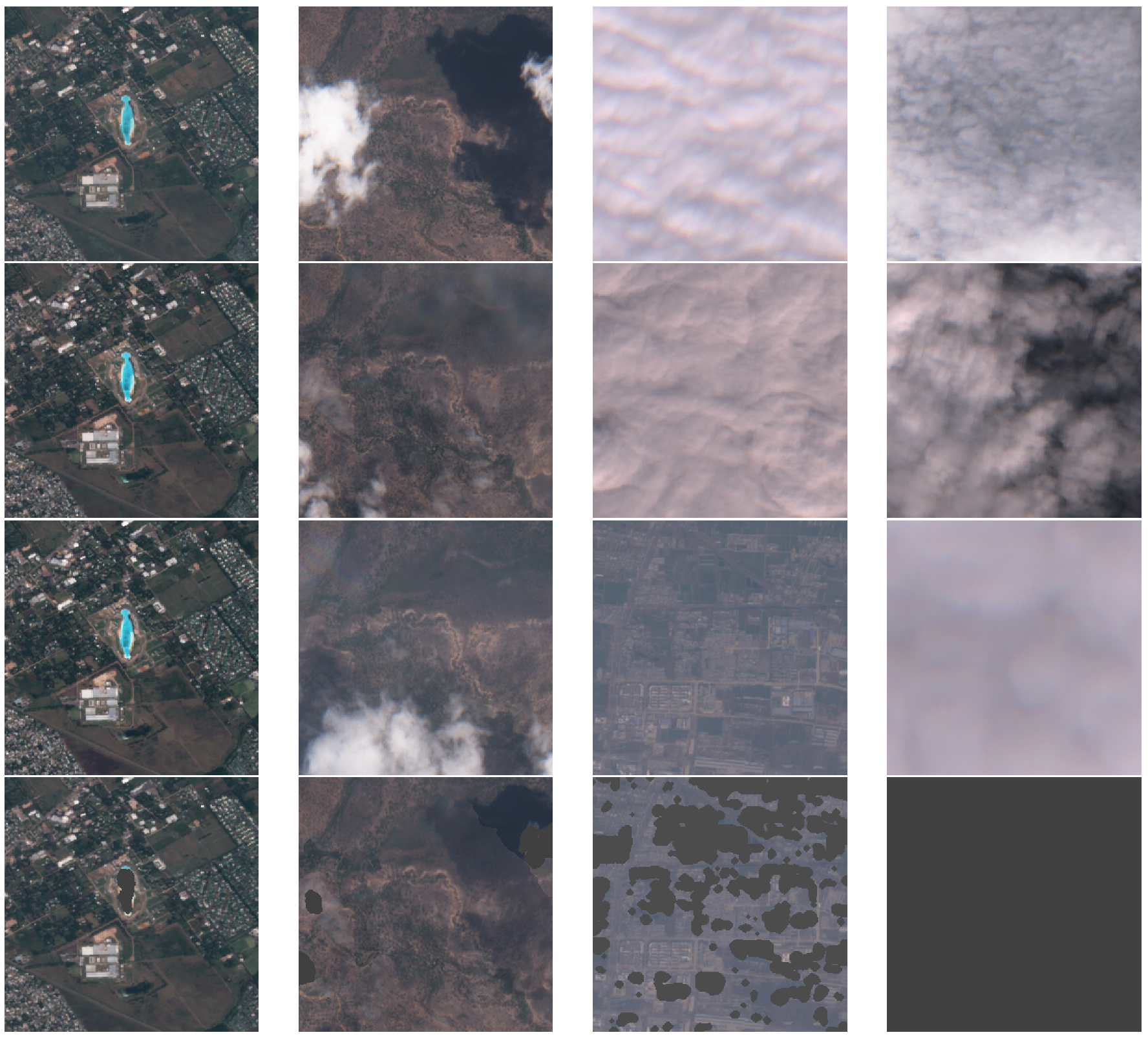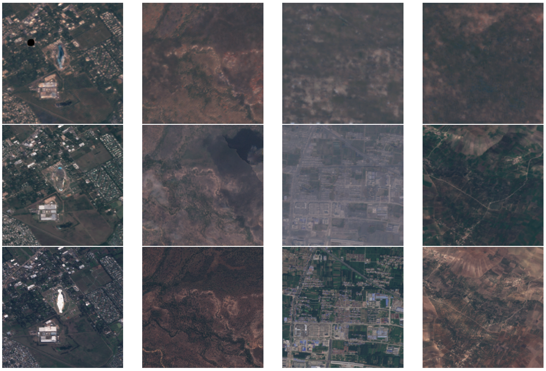The examples of the reconstructed outcomes for the considered baselines on four different samples from the test split are illustrated in Figure 3. The considered cases are cloud-free, partly cloudy, cloud-covered with no visibility except for one single time point, and cloud-covered with no visibility at any time point. The illustrations show that SeqDMs can perfectly maintain any cloud-free pixels of the input sequences and leverage the distribution of the known regions to generate the cloudy pixels.

However, SeqDMs fall short of capturing the imagery structure or multi-spectral structure when the input sequences are quiet short, in terms of SSIM and SAM metrics. The input sequences are quite short, indicating that input samples are collected in a relatively concentrated period. This produces three challenges for the cloud removal using SeqDMs with the powerful ability of distribution capture: (1) Cloud coverage might be quiet high, resulting in severe information loss. (2) The temporal shift between input samples and cloud-free target image might be large, causing significant differences in the perceived change, contrast, or luminance. (3) The robustness of exceptional data due to equipment failure might be weak, misleading the model to a wrong inference direction that is completely different from the cloud-free target image.

To overcome the above challenges, we consider the inference process (i.e., cloud-removal process) over longer input sequences by using the conditional inference strategy detailed in Section 3.2.2 to integrate more information across time without retraining the SeqDMs again.

Table 2. Quantitative evalutation of the proposed method SeqDMs and Seq2point [7] inferred with input sequences of length $L=3,4,5$ in terms of NRMSE, PSNR, SSIM [31], and SAM [32] metrics. It is worth noting that SeqDMs need to be trained only once with sequences of length $L=3$, while Seq2point [7] needs to be trained with sequences of length $L=3,4,5$, respectively.

Model	NRMSE(All) ↓	NRMSE(Cloudy)	NRMSE(Clear)	PSNR ↑	SSIM ↑	SAM ↓
Seq2point (L = 3)	0.051	0.052	0.040	26.68	0.836	0.186
SeqDMs (L = 3)	0.045	0.046	0.026	28.07	0.827	0.223
Seq2point (L = 4)	0.049	0.050	0.041	27.10	0.845	0.172
SeqDMs (L = 4)	0.037	0.038	0.024	28.31	0.847	0.201
Seq2point (L = 5)	0.048	0.048	0.032	27.07	0.846	0.178
SeqDMs (L = 5)	0.038	0.038	0.017	28.21	0.846	0.198

The ↓ means lower is better, and ↑ means the higher is better.

reports the performance of our proposed method SeqDMs and Seq2point [7] inferred with input sequences of length $L=3,4,5$, respectively. It is worth noting that SeqDMs need to be trained only once with sequences of length $L=3$, while Seq2point [7] needs to be trained with sequences of length $L=3,4,5$, respectively. The results indicate that inferring with longer input sequences can significantly improve the performance of SeqDMs in terms of reconstructed quality, imagery structure, and multi-spectral structure and can easily outperform the baseline methods in majority metrics with much less training cost, except for SAM.

To further understand the benefit of conditional inference strategy,

Table 3. Performance of our proposed method SeqDM as a function of cloud coverage, inferred with input sequences of length $L=3,4,5$. The cloud coverage is calculated by averaging the extent of clouds of each images in the sequence of length $L=3$.

Cloud Coverage	L	NRMSE(All) ↓	NRMSE(Cloudy)	NRMSE(Clear)	PSNR ↑	SSIM ↑	SAM ↓
0–10%	3	0.023	0.030	0.023	32.31	0.907	0.118
	4	0.024	0.028	0.021	31.81	0.905	0.120
	5	0.024	0.026	0.015	31.74	0.907	0.120
10–20%	3	0.035	0.035	0.034	28.00	0.863	0.161
	4	0.034	0.033	0.038	28.17	0.865	0.160
	5	0.033	0.033	0.029	28.48	0.871	0.157
20–30%	3	0.033	0.032	0.034	29.30	0.854	0.138
	4	0.032	0.032	0.038	29.25	0.855	0.138
	5	0.032	0.031	0.021	29.61	0.861	0.135
30–40%	3	0.033	0.032	0.032	29.86	0.875	0.156
	4	0.033	0.033	0.028	29.08	0.873	0.160
	5	0.033	0.033	0.027	29.08	0.875	0.160
40–50%	3	0.045	0.045	0.042	26.54	0.826	0.227
	4	0.042	0.042	0.037	26.96	0.834	0.223
	5	0.042	0.042	0.034	26.93	0.834	0.222
50–60%	3	0.042	0.042	0.023	28.40	0.832	0.217
	4	0.041	0.041	0.020	27.91	0.841	0.217
	5	0.041	0.041	0.030	27.91	0.841	0.217
60–70%	3	0.038	0.038	0.029	29.36	0.838	0.217
	4	0.038	0.038	0.024	27.88	0.839	0.220
	5	0.040	0.040	-	27.68	0.832	0.220
70–80%	3	0.048	0.048	-	24.60	0.803	0.268
	4	0.040	0.040	-	27.13	0.842	0.228
	5	0.045	0.045	-	26.68	0.822	0.225
80–90%	3	0.050	0.050	-	24.58	0.779	0.285
	4	0.038	0.038	-	28.60	0.834	0.216
	5	0.040	0.040	-	28.48	0.833	0.209
90–100%	3	0.104	0.104	-	18.80	0.609	0.434
	4	0.059	0.059	-	24.52	0.755	0.288
	5	0.054	0.054	-	24.96	0.782	0.261

The ↓ means lower is better, and ↑ means the higher is better.

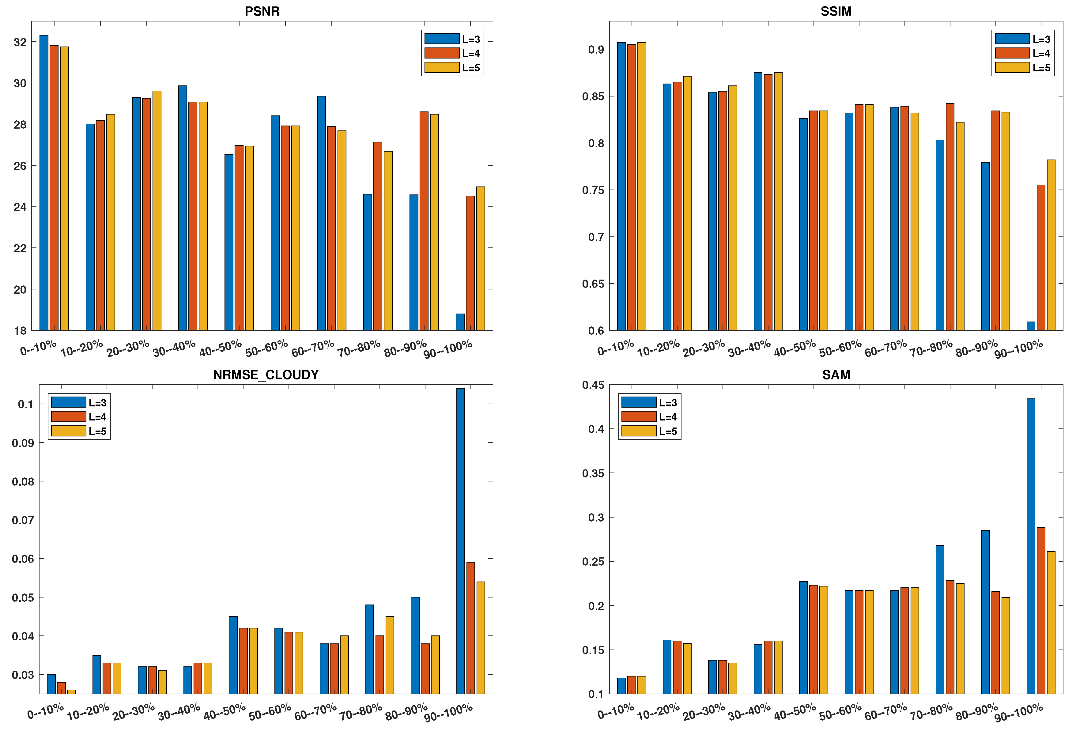
reports the performance of SeqDMs as a function of cloud coverage, inferred with input sequences of length $L=3,4,5$. The cloud coverage is calculated by averaging the extent of clouds of each images in the sequence of length $L=3$. The results show that longer input sequences can significantly improve the performance, especially in the cases of extreme cloud coverage. Figure 4 shows the performance histograms of SeqDMs in terms of PSNR, SSIM, NRMSE(cloudy), and SAM; it visualizes the significant improvements in the extreme cloud coverage cases by increasing input sequences length L. In addition, the cloud-removal performance is highly dependent on the percentage of the cloud coverage. While the performance decrease is not strictly monotonous with an increase in cloud coverage, a strong association still persists.

Finally, we conduct an ablation experiment to assess the benefit of utilizing the temporal training strategy of SeqTIS.

Table 4. Comparison of the proposed method SeqDMs ($L=3$) using the temporal training strategy of SeqTIS versus an ablation version not using the temporal training strategy (i.e., only trained with Equation (27)) in terms of NRMSE, PSNR, SSIM [31], and SAM [32] metrics.

Model	NRMSE(All) ↓	NRMSE(Cloudy)	NRMSE(Clear)	PSNR ↑	SSIM ↑	SAM ↓
SeqDM (no temporal training strategy)	0.048	0.050	0.026	27.90	0.821	0.223
SeqDM (with temporal training strategy)	0.045	0.046	0.026	28.07	0.827	0.223

The ↓ means lower is better, and ↑ means the higher is better.

compares the results of our propose method SeqDMs with an ablation version not using temporal training strategy (i.e., only trained with Equation (27)). The comparison demonstrates that using the whole version of temporal training strategy of SeqTIS leads to a higher quality in the cloud-removal task.

5. Discussion

The main contribution of this paper is in the development of the sequential-based diffusion models (SeqDMs), which is a novel probabilistic generative model for the cloud-removal task of optical satellite imagery. It consists of two parts, multi-modal diffusion models (MmDMs) and sequential-based training and inference strategy (SeqTIS). MmDMs are novel diffusion models that reconstruct the reverse process of DDPMs to integrate additional information from the auxiliary modalities (e.g., SAR or other modalities robust to the corruption of clouds or haze) in order to help the distribution learning of the main modality (i.e., optical satellite imagery). Although the main modality typically is susceptible to the influences of clouds or haze, MmDMs are capable of capturing the distribution of the main modality by conditioning the missing information with the auxiliary modalities during the training and inference process. SeqTIS is an improved training and inference strategy specifically for MmDMs, which allows us to integrate temporal information across arbitrary length of the both main modality and auxiliary modalities input sequences without retraining the model again. With the help of the MmDMs and SeqTIS, our proposed method SeqDMs outperform several other state-of-the-art multi-modal multi-temporal cloud removal methods and have the flexibility to handle the arbitrary length of input sequences, producing significant improvements with only one or two additional input samples and greatly reducing the time cost of model training, as detailed in Table 1 and Table 2. This work serves as an important stepping stone for cloud removal by integrating information across time and data modalities to achieve improved interpretability, model flexibility, and generalizability. However, due to the powerful distribution capture capability of MmDMs and the direct information combination of known regions and unknown regions by SeqTIS, knowing how to more effectively enhance the robustness of the exceptional data in sequence and more efficiently extract useful information based on the transparency of the cloud is still crucial to fundamentally improve the performance of the proposed method rather than inferring over longer input sequences.

6. Conclusions

This paper proposes SeqDMs, a novel probabilistic generative model for the cloud-removal task in remote sensing. Unlike other popular generative models, our method introduces a novel diffusion model by reconstructing the reverse process of DDPMs to integrate additional information from the auxiliary modalities and utilizes a specialized training and inference strategy to handle sequences of an arbitrary length without retraining the model again. Our extensive experiments demonstrate that our method outperforms several state-of-the-art methods in cloud removal with excellent interpretability and flexibility. In the future, we will pursue the direction of studying the characteristics of each band of the multi-spectral optical satellite imagery to extract more helpful information for further reducing the semantic gap between the reconstructions and target images.