Article

Forest Vertical Structure Mapping Using Multi-Seasonal UAV Images and Lidar Data via Modified U-Net Approaches

1
Department of Geoinformatics, University of Seoul, 163 Seoulsiripdae-ro, Dongdaemun-gu, Seoul 02504, Republic of Korea
2
Department of Smart Cities, University of Seoul, 163 Seoulsiripdae-ro, Dongdaemun-gu, Seoul 02504, Republic of Korea
*
Author to whom correspondence should be addressed.
Remote Sens. 2023, 15(11), 2833; https://doi.org/10.3390/rs15112833
Submission received: 19 March 2023 / Revised: 1 May 2023 / Accepted: 27 May 2023 / Published: 29 May 2023

Abstract

:
With the acceleration of global warming, research on forests has become important. Vertical forest structure is an indicator of forest vitality and diversity. Therefore, further studies are essential. The investigation of forest structures has traditionally been conducted through in situ surveys, which require substantial time and money. To overcome these drawbacks, in our previous study, vertical forest structure was mapped through machine learning techniques and multi-seasonal remote sensing data, and the classification performance was improved to a 0.92 F1-score. However, the use of multi-seasonal images includes tree location errors owing to changes in the timing and location of acquisition between images. This error can be reduced by using a modified U-Net model that generates a low-resolution output map from high-resolution input data. Therefore, we mapped vertical forest structures from a multi-seasonal unmanned aerial vehicle (UAV) optic and LiDAR data using three modified U-Net models to improve mapping performance. Spectral index maps related to forests were calculated as optic images, and canopy height maps were produced using the LiDAR-derived digital surface model (DSM) and digital terrain model (DTM). Spectral index maps and filtered canopy height maps were then used as input data and applied to the following three models: (1) a model that modified only the structure of the decoder, (2) a model that modified both the structure of the encoder and decoder, and (3) a model that modified the encoder, decoder, and the part that concatenated the encoder and decoder. Model 1 had the best performance with an F1-score of 0.97. The F1-score value was higher than 0.9 for both Model 2 and Model 3. Model 1 improved the performance by 5%, compared to our previous research. This implies that the model performance is enhanced by reducing the influence of position error.

1. Introduction

Recently, the importance of forests has been emphasized because of the acceleration of global warming [1]. According to the intergovernmental panel on climate change (IPCC), forests could absorb 12–15% of the greenhouse gas emissions that cause global warming, and forests also protect the Earth’s ecosystems from the effects of extreme weather events [2,3]. Owing to their importance, forests are being continually investigated. The vertical forest structure is a hierarchy created by differences in the height of vegetation [4]. It is an indicator of vegetation diversity and vitality and is used to monitor forests [5]. Traditionally, forest structure is classified through field surveys. This requires significant resources, including time, money, and labor, especially in mountainous areas, and some areas are inaccessible. Thus, field surveys of forest structures could not be investigated in the entire area of interest, and it is difficult to update the data quickly [6,7]. Remote sensing has been used to overcome these limitations [8]. Remote sensing data capture electromagnetic waves that are reflected or emitted from the surface and contain physical information about a large area [9]. Spectral indices are generated using specific wavelength bands to allow for in-depth forest research [10]. Remote sensing data has advantages in terms of time and cost compared to field surveys because the data is acquired remotely and periodically for a wide region. However, as it obtains data indirectly, this approach tends to be less accurate than field surveys [11]. To supplement this, remote sensing data has been applied to deep learning techniques.
Deep learning is a machine learning algorithm that attempts to achieve a high level of abstraction by combining multiple nonlinear converter methods and is useful for detecting complex structures in large datasets [12,13]. Deep learning has advanced rapidly in response to increases in computing power and the availability of big data and exceeds the performance of traditional algorithm-based methods [14]. In addition, deep learning has been employed to investigate the vertical structure of forests [15]. Lee et al. [16] generated a topographic and normalized spectral index map from aerial images to reduce topographic errors in mountainous locations and then applied it to an artificial neural network (ANN) to classify forest structures.
In our previous study [17], we applied machine learning techniques to multi-seasonal data acquired from an unmanned aerial vehicle (UAV) to improve the classification performance of forest structures by a 0.92 F1-score. However, this study could not consider spatial characteristics in model training because the model was trained and predicted pixel by pixel, and the tree position error between two period images contained in the multi-seasonal data could not be considered. Since UAV platforms are vulnerable to wind speed, wind direction, aircraft attitude, altitude, and other factors, the tree location of time series data was captured differently in the same site [18,19]. The difference in the locations is an error component in model learning and reduces the performance of the model. These problems can be solved by using a modified U-Net.
U-Net is a model that extracts image context and local information from a large number of image pixels, classifies objects based on them, and consists of encoder and decoder structures [20]. The decoder of U-Net provides a detailed localization on the feature map generated by the encoder by convolution and up-sampling. The encoder applies a convolution filter to each channel of the input map and creates a single feature map by combining the calculated value to all channels [21,22]. This causes a loss in the independent characteristics of each input map. This loss of independent features can be reduced by a deep learning model structure with multiple encoder branches based on the features of each channel [23]. In addition, reducing the up-sampling operation of the decoder corrodes the localization information of the output map. By generating a low-resolution output map that is less sensitive to position errors using high-resolution input data, it is possible to minimize the position error components between the two periods.
In the present study, we trained the model and analyzed its effects by minimizing location errors using multi-season data and a modified U-Net structure. We acquired two periods of UAV optic and Lidar data and utilized them to generate a spectral index and a filtered canopy height map. The preprocessed data were then applied to three different U-Nets: (1) a model with only the decoder structure modified, (2) a model with the encoder and decoder modified, and (3) a model that modified the encoder, decoder, and their connection. The performance of mapping the vertical forest structure was then calculated, evaluated, and analyzed.

2. Study Area and Data

The study area is located in Samcheok-si, Gangwon-do, South Korea, which is a coastal city on Taebaek Mountain. The region has a moderate climate with four distinct seasons, with an average annual temperature of 13.2 °C and precipitation of 1159 mm. The region is affected by anthropogenic interference, with a mix of artificial and natural forests, softwoods and hardwoods. In addition, it is dominated by natural forest Rhododendron mucronulatum and Pinus densiflora and mixed-in alien species of artificial forest Pinus rigida and Robinia pseudoacacia. Figure 1b shows the vertical forest structure map used for the ground truth in this study. The vertical forest structure map was obtained through an in situ survey. Forest structures are known to have four layers in temperate regions [24]. However, in this area, the range is small and consists of three-layered structures: one-, two-, and four-storied. A one-storied forest consists of a canopy and includes Robinia pseudoacacia and Alnus japonica. The two-storied forest consists of a canopy and shrubs and includes Toxi-codendron vernicifluum, Zanthoxylum piperitum, Rhododendron mucronulatum, Quercus mongolica, Pinus densiflora, R. pseudoacacia, and Platycarya quercus serrata. The four-storied forest consists of herbaceous, shrub, understory, and canopy, including Festuca ovina, Z. piperitum, R. mucronulatum, T. vernicifluum, Q. serrata, and Pinus densiflora.
The data used in this research were acquired from two periods of optical images, LiDAR data obtained from sensors mounted on the UAV, and DTM data provided by the National Geographic Information Institute (NGII). The first UAV data were acquired on 22 October 2018 (fall), and the second UAV data were acquired on 29 November 2018 (winter). The temperature difference between the two dates in the region was 8.3 °C, and the deciduous period was included between the two periods [25]. The trees showed different characteristics before and after the leaf fall. Therefore, we intended to reflect the characteristics of seasonal changes through the images of the two dates.
The flight altitude of the UAV was 200 m, the overlap between the lateral and longitudinal directions was 80%, and the scanning time was approximately 46 min. Optical images were acquired using an RX02 camera and had a total of five band bands (Table 1): blue, green, red, red edge, and near-infrared (NIR). Optical images were geometrically corrected using automatic aerial triangulation. Their spatial resolution was 21–22 cm, which was resampled to 20 cm using cubic interpolation. Table 2 lists the specifications of the LiDAR sensors. A Velodyne Lidar Puck (VLP-16) sensor was used to acquire point cloud data for the LiDAR data, and a DSM was produced. The LiDAR-derived DSM was produced by filtering the point cloud data into a grid. The spatial resolution of the DSM was approximately 2 cm, which was resampled to 20 cm. The DEM was also intended to be produced through the LiDAR point cloud. However, the area was densely forested and could not be reproduced. Therefore, the DTM provided by NGII was used. The NGII DTM has a resolution of 5 m, but it uses numerical topographic data created by contour lines. In general, the surface of the terrain can be approximated as a smooth surface; therefore, it was used by resampling 5 m of data to 20 cm.

3. Methodology

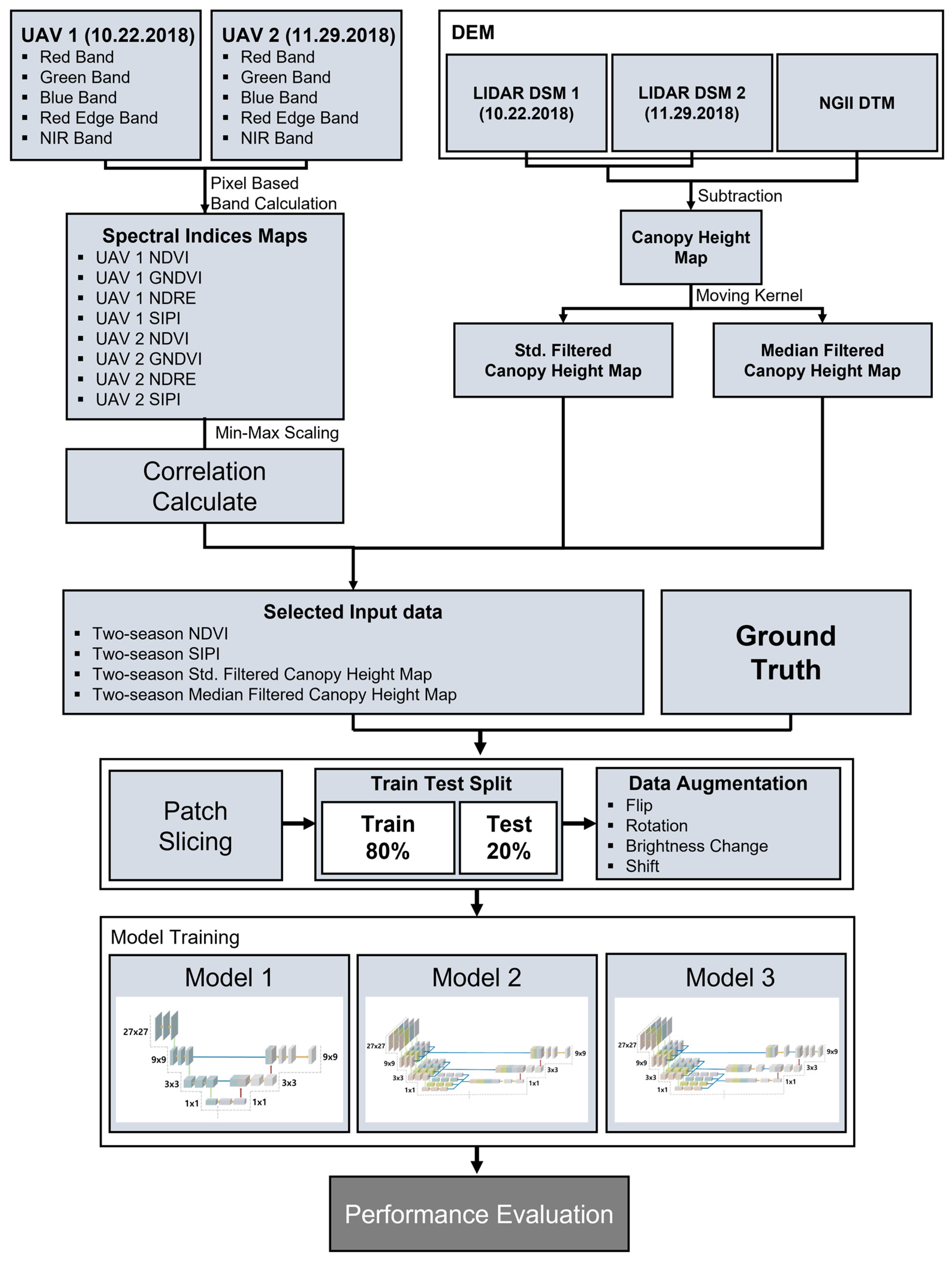
To analyze the effect of learning the model by reducing the tree position error component of the image, three modified U-Net models were produced and trained using preprocessed data. Subsequently, a quantitative performance evaluation was conducted using the test dataset. Figure 2 shows the detailed workflow of this study, which can be largely divided into three parts: (1) data preprocessing, (2) patch slicing and data augmentation, and (3) model training and performance comparison analysis.

3.1. Generation of the Normalized Input Data

3.1.1. Spectral Index Maps

The spectral index map calculated by the spectral characteristics of the remote sensing image is used to analyze the physical characteristics of the Earth’s ecosystem, such as vegetation and water resources [26]. This map reduces distortion components of topography and shadows that act as errors in optical images in quantitatively analyzing and evaluating the Earth’s surface [27,28]. The errors are reduced through pixel-based band ratio calculation; therefore, the spectral index map was used as input data for effective vegetation analysis [29]. For effective vegetation analysis, spectral indexes produced a total of four types: NDVI, GNDVI, NDRE, and SIPI, calculated using the values of the visible, red edge, and NIR bands. Table 3 lists the formulae for the spectral indices used in this study.
NDVI is a vegetation index that was developed to focus on high reflectance in healthy, energetic, or dense vegetation [30]. It uses red and NIR band images to evaluate the vitality and density of the vegetation. The GNDVI uses green band images instead of red band images in the NDVI equation, which represents the sensitivity of vegetation to chlorophyll changes [31]. Variations in the nitrogen content of leaves can be detected using the GNDVI. NDRE is an index that uses red-edge bands instead of red bands to respond more sensitively to changes in plant health and vitality [32]. The SIPI is an effective index for assessing vegetation composed of multiple layers [33]. It was calculated by computing the ratio of chlorophyll carotenoids in the blue, red, and near-infrared bands. The higher the stress of the vegetation, the higher the SIPI. Machine learning algorithms find patterns by analyzing and comparing features between different data [34]. Substantial differences in the range and unit of each feature in the dataset can make it difficult to train the model correctly [35]. Thus, the four spectral index maps were normalized to the range of values from 0–1 with min–max scaling to avoid problems and improve model performance. Subsequently, the input data were selected using correlation calculation. Utilizing two highly correlated datasets as deep-learning input data produced the same results. This increases the model size, which not only decreases computing speed but also diminishes the explanatory power of the model. For this reason, two low-correlation datasets were selected as input data. The correlation coefficient was defined as follows [36]:
C o r ( I m a g e   1 ,   I m a g e   2 ) = C o v ( I m a g e   1 , I m a g e   2 ) V a r ( I m a g e   1 ) V a r ( I m a g e   2 )  

3.1.2. Filtered Canopy Height Maps

The vertical structure of the forest is strongly related to the height of the growing plants. Multi-layered structures have coarse image texture characteristics and reflectivity variation due to height differences with the surrounding individual trees. However, single-layered forests have monotonous image texture because of their similar arrangement of trees [37]. To reflect this in the model, a canopy height map was created by subtracting the NGII DTM from LiDAR-derived DSM. The DSM indicates a height that includes all natural and artificial objects, and the DTM is numerical topographic data created by contour lines, representing the height of the topographic surface. Thus, canopy height data can be obtained by subtracting DTM from DSM. To represent this statistically, the canopy height was filtered with a median and standard deviation kernel of 51 × 51 [38]. Kernel size was determined by factoring in the area (10 m × 10 m) used in the forest survey. The median filtered canopy height map represents the central tendency of tree height, whereas the standard deviation filtered canopy height map represents the amount of variance in tree height. Identical to the spectral index map, min–max scaling was applied to the two filtered canopy height maps.

3.1.3. Patch Slicing and Data Augmentation

U-Net utilizes patch-based data as input [39]. Compared to the pixel-based model, the patch-based model has the advantage of reflecting spatial characteristics [40]. The selected input and label data were split into a 35 × 35 patch format for input into the model, reflecting spatial properties. The patch was split into 80% of the training set and 20% of the test set to avoid overlap. UAV data has high-resolution characteristics, but the amount of data available is limited as the acquisition area is smaller than that of satellite images and is not acquired on a regular basis [41]. Training the model with a variety of datasets aids in preventing overfitting to new datasets and ensuring robustness to new datasets [42]. Therefore, data augmentation was applied to training patches produced to increase the amount and diversity of data by flip, rotation, shift, and brightness change methods. The data were doubled using the upper, lower, left, and right flips of the patch. The patch was also rotated to [15°, 75°, 90°, 105°, 165°, 180°, 195°, 255°, 270°, 285°, and 345°] and increased 11 times. Following this, the augmented patch was shifted by one pixel and two pixels, up, down, left, and right, respectively, to increase the data by a multiple of eight. The brightness change was then applied to the expanded patch. For information on the change in brightness of the image, including vegetation, refer to the paper by Mäyrä et al. [43], and the equation is as follows:
x a u g = σ ( l o g i t ( x ) + l o g i t ( c h a g e 0.5 ) ) ,   σ ( x ) = e x e x + 1 ,   l o g i t ( x ) = log ( 1 x 1 )
where x is the min–max normalized data, and σ(x) represents the sigmoid function. Logit (x) refers to the logit function, and the change value used in the logit function is random among the values of [0.8, 1.2]. After data augmentation, the selected spectral index and filtered canopy height maps were cropped into a 27 × 27 patch in the middle to remove null values caused by rotation. This was used as input data for the model. Moreover, the size of the output is smaller than the model input due to minimizing the positional error by reducing the up-sampling process in the model structure. To consider this, the ground truth was cut into 9 × 9 patches in the middle and used for label data. The quantity of data for the one-storied class was less than that of the two- and four-storied. An imbalance of pixels in each class can cause overfitting. To solve this problem, we used an oversampling method to increase the number of one-storied class pixels. Finally, 591,000 augmented patches were used for model training and 1000 patches were used for testing.

3.2. Training Model

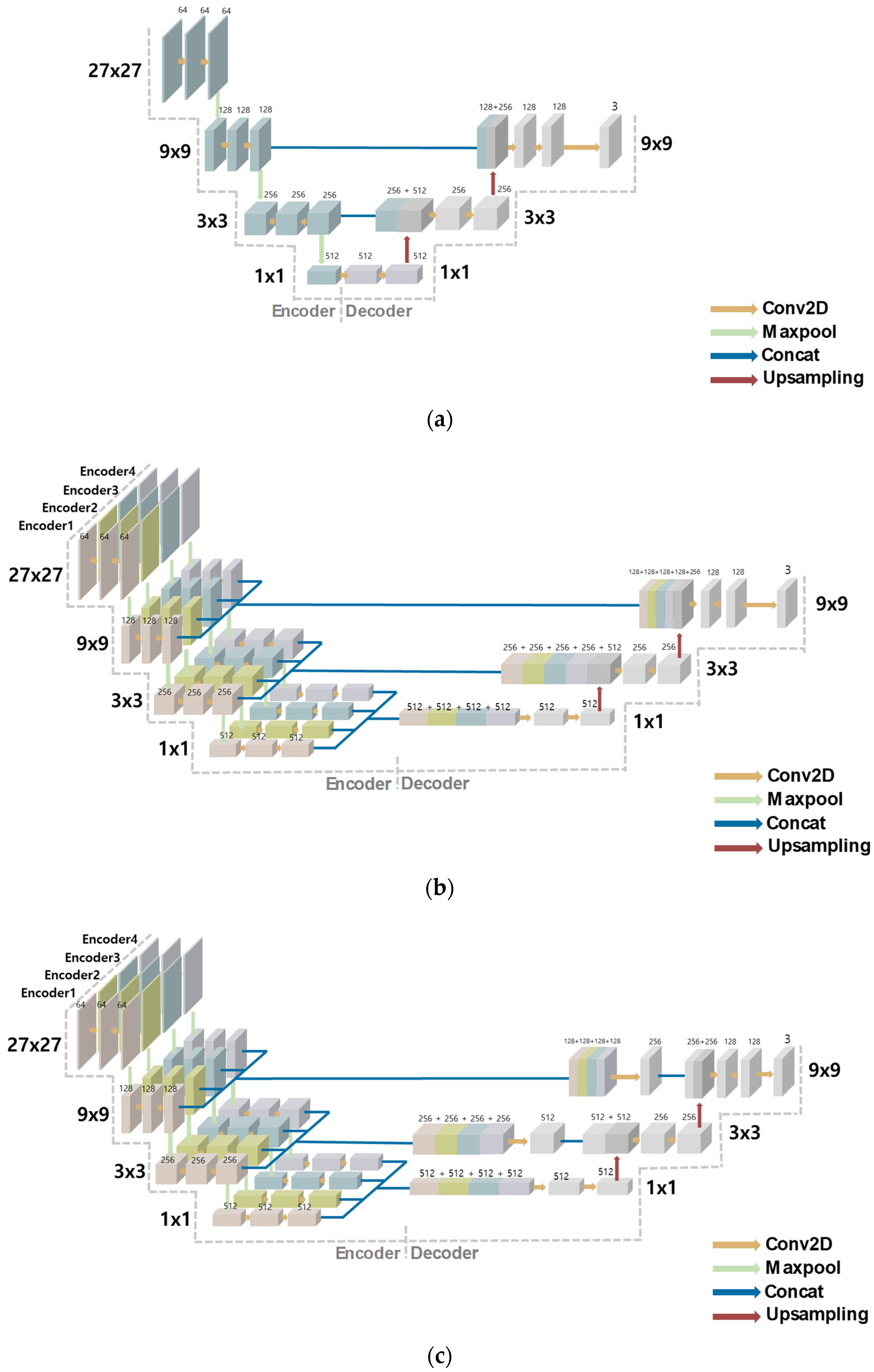
The 591,000 training patches generated were applied to the three modified U-Nets. Deep-learning models produce different results depending on how the structure of the model is configured. To determine which model is best for predicting the vertical structure of a forest, we chose to configure the model structure differently. Figure 3 shows the structure of the three U-Net models used in this study. Model 1 is shown in Figure 3a, and the encoder was the same as the original U-Net structure, but the decoder structure was modified. In contrast to the original U-Net decoder, it was not up-sampled to the same size as the input patch size, and its output size was 9 × 9. By generating a low-resolution output from high-resolution input data, the effect of tree position errors between images from the two periods can be reduced. Model 2 is illustrated in Figure 3b and it additionally modified the encoder structure of Model 1. The encoder of the existing U-Net comprises only a single path. Each channel of the input data is applied to a convolution filter, and the values calculated for all channels are combined to generate a characteristic map. However, the problem with this process is that the independent characteristics of each channel are lost. To reflect the unique features of each channel in the model, the existing structure of one path was changed to a multi-encoder with four paths. Figure 3c represents Model 3. Model 3 has the same encoder and decoder structure as Model 2; however, it is different from the feature map derived from the encoder that performs additional convolution operations before being transmitted from the decoder to match the channel of the decoder feature map.

3.3. Performance Evaluation

After training the model, a confusion matrix between the predicted result and ground truth was produced using the test dataset. The precision, recall, precision-recall (PR) curve, and F1-score were produced using a confusion matrix, and the model was quantitatively analyzed. Precision refers to the proportion of actual true pixels among those classified as true by the trained model, while recall refers to the fraction of actual true pixels retrieved by the trained model. The formulas for precision and recall are as follows [44]:
P r e c i s i o n = T r u e   P o s i t i v e T r u e   P o s i t i v e + F a l s e   P o s i t i v e
R e c a l l = T r u e   P o s i t i v e T r u e   P o s i t i v e + F a l s e   N e g a t i v e
Precision and recall have a trade-off [45]. Therefore, to comprehensively compare and evaluate the performance of the model, the entire performance change in precision and recall must be considered. The PR curve confirms this finding. The PR curve represents the change in the precision and recall values as the algorithm parameters are altered. The PR curve has an average precision (AP) value, which is derived using the bottom area of the graph line and is used as a measure of model classification performance. The higher the AP value, the more adept the model is at classification [46]. The F1-score is an indicator that integrates the trade-off between precision and recall and represents the performance of the model as a single value. It is derived as the harmonized average of the two values. The F1-scores are defined as follows [47]:
F 1   s c o r e = 2 P r e c i s i o n R e c a l l P r e c i s i o n + R e c a l l

4. Results

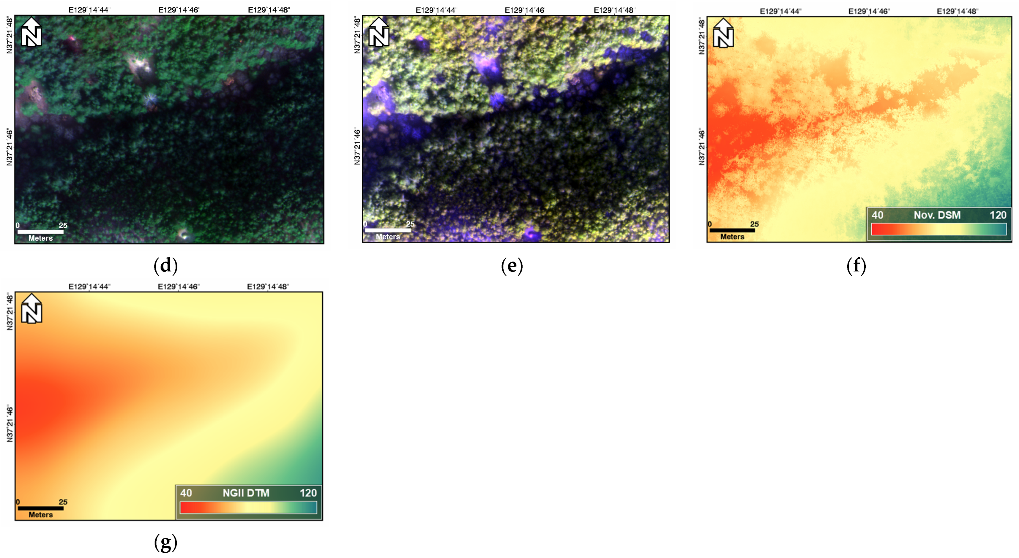
Figure 4 shows the true color (red, green, and blue band composite) images, false color (red edge, NIR, and blue band composite) images, LiDAR DSM, and NGII DEM used in this study. It is difficult to distinguish between the one-, two-, and four-storied in all images using visual analysis. Compared to the images acquired in October, those acquired in November were relatively dark. Figure 4d,e is identified more clearly for a one-storied structure than Figure 4a,b. This is because the one-storied region is more responsive to seasonal changes than the multistoried region. The values shown in Figure 4f are lower than that of Figure 4c, as the height of the tree decreases because the leaves of vegetation fall as the seasons change.
Table 4 shows the results of the correlation coefficients among the spectral indices. The correlation coefficient between the GNDVI and NDVI was 0.825, which was the highest. This is because GNDVI analyzes vegetation vitality using the adjacent green band instead of the red bands in the NDVI equation. Among the spectral indices, the data with the lowest correlation had a value of −0.27 as NDVI and SIPI. The NIR and red bands were used for both indices. However, the SIPI calculation equation additionally included the blue band. Based on the results, NDVI and SIPI with low correlations were selected as the input data for the model.
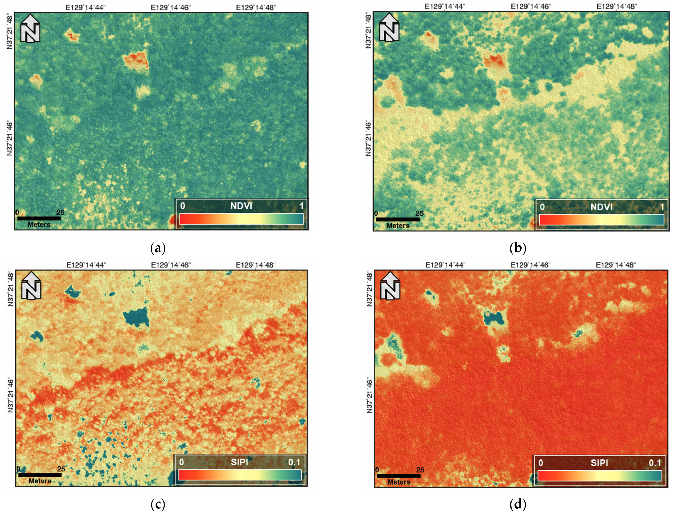
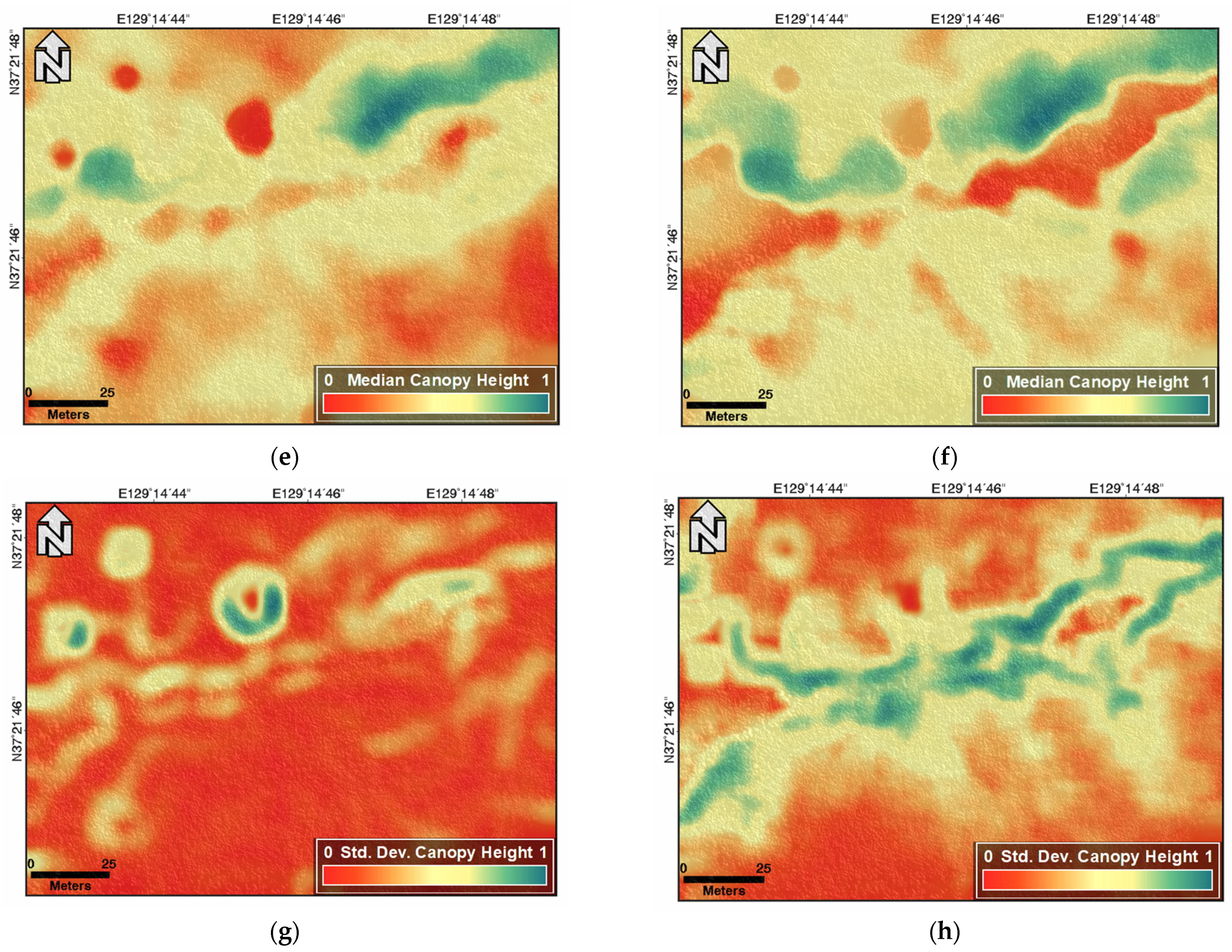
Figure 5 shows the normalized NDVI and SIPI selected through the correlation between the two periods and the canopy height map filtered by the median and standard deviation. The normalized spectral index map does not include shadow effects from topography in the image, as opposed to the true color composite and false color composite images in Figure 4. This is because the effect of topography is reduced when calculating the pixel-based band ratio. Therefore, spectral indices were used as the input data for deep learning instead of optical images. The index map of November has a significantly different value than that of October, which is due to seasonal changes. Figure 5b,d have lower values than those shown in Figure 5a,c because the decrease in temperature causes leaves to fall off, reducing the impact of the trees. Compared to October NDVI, November NDVI showed a clear difference in forests on the first, second, and fourth floors. However, in SIPI, the value distribution of the October index appears to vary more. Figure 5e–h shows filtered canopy height maps. Tree height is closely related to the vertical structure of the forest. Because the spectral index alone lacks explanatory power for the vertical forest structure, filtered height data were also employed. The images filtered by the median and standard deviation tended to be similar to the vertical structure of the forest. Furthermore, the canopy height map derived from LiDAR, such as the spectral index, is affected by the decrease in leaves, and the November image has a pattern that is more evident on the one-, two-, and four-storied images than on the October images. As shown in Figure 5h, the four-storied forest has a high standard deviation value. This implies that trees of various heights exist in the four-storied.
Following the generation of the two-season data in patch form, the amount of training data set was increased and applied to the three modified U-Nets. All three models were trained using common hyperparameters. The model optimization function used Adam, and the learning rate, which is the optimization ratio, was changed from 1 × 10⁻³ to 5 × 10⁻⁵. Additionally, the value of the loss was derived using the sparse category cross-entropy function. The batch size refers to the number of data to collect gradients from one backpropagation, which was set to 1000, and repeated learning was conducted by setting the epoch to 1000.
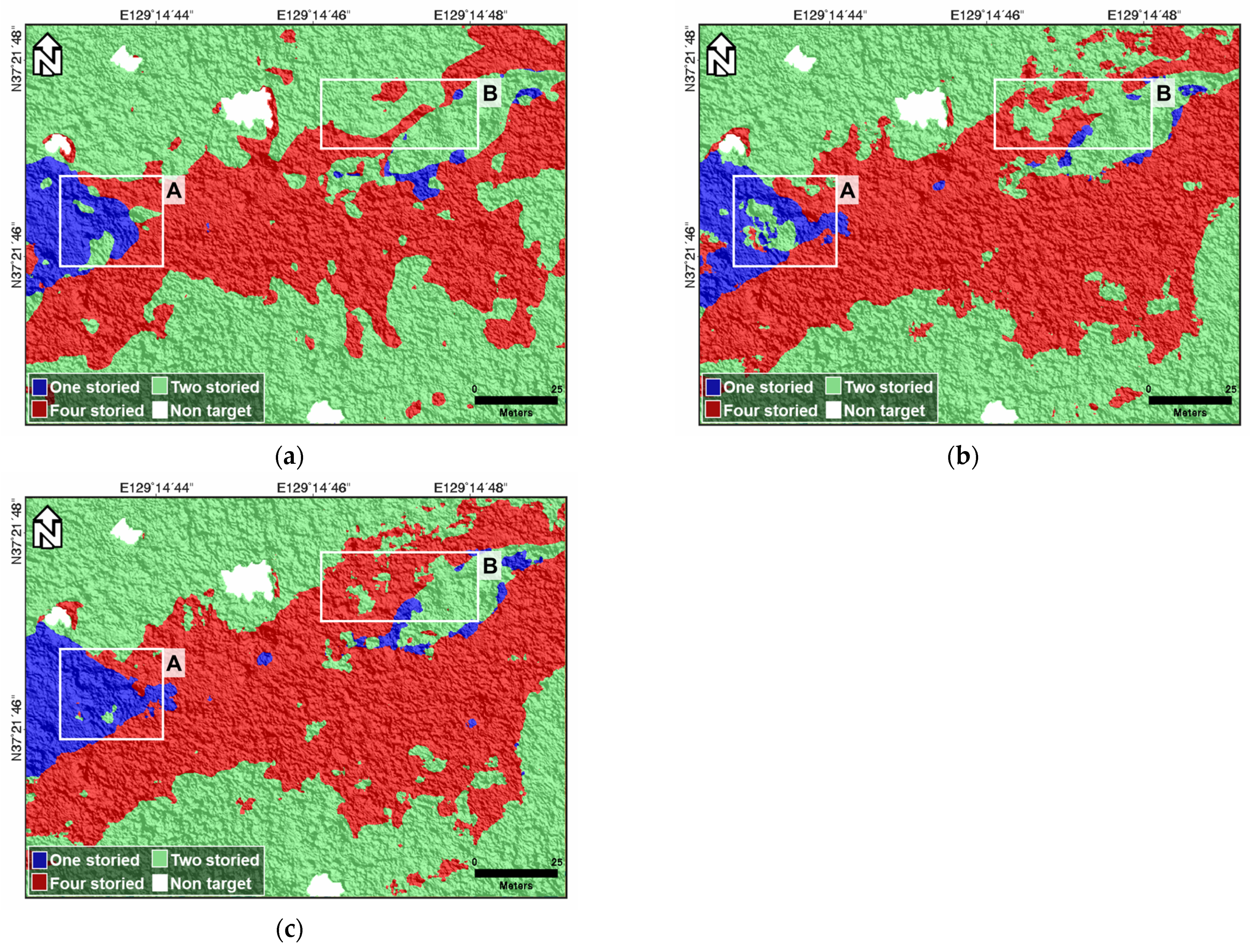
Figure 6 shows the forest structure map estimated using the three modified U-Net models. All the predicted maps tended to be similar to the ground truth. All three maps appear as boundaries between the lumped layers. This is because the map was not predicted based on the value of each pixel but was derived through patch-based input data. Moreover, the boundary between floors was smoothed. By modifying the up-sampling structure of the decoder, a low-resolution output was predicted from the high-resolution input, decreasing the positional error between the two periods of data. The visual analysis shows that Model 3 is the most similar to the ground truth, and Model 1 is the worst. This can be seen in more detail in Box A and Box B. The significant differences identified in Box A are as follows: (1) in Model 3, the one-storied structure is clearly classified, whereas in Models 1 and 2, two-storied structures exist frequently in the one-storied part. (2) Model 3 represents a clear boundary between stories one and two, whereas Models 1 and 2 depict a disturbed boundary between all stories. In Box B, Model 3 properly classified the four-storied into the four-storied, but Models 1 and 2 predicted the two-storied structure. Overall, two- and four-stories appear to be confused in Models 1 and 2, respectively.
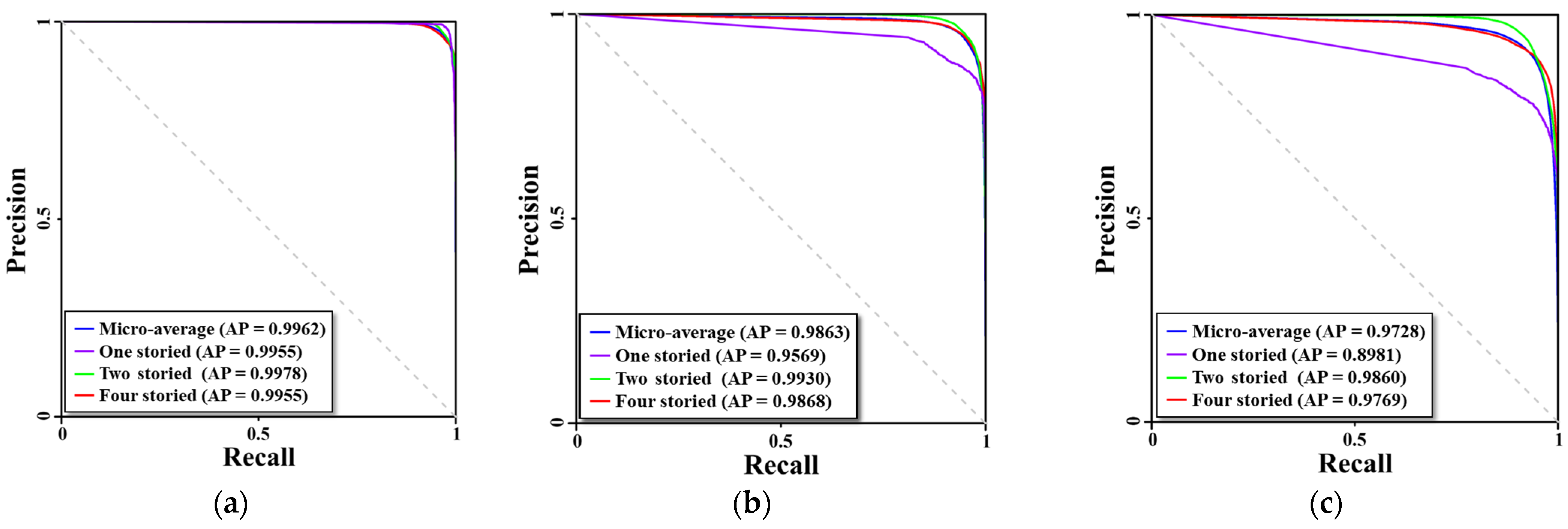
The forest vertical structure maps in Figure 5 were created using both the training data and test data. The training data was directly used for deep learning model convergence and is not adequate to evaluate the general performance of the model. Therefore, the test dataset was applied to the trained model and quantitative analysis was performed to evaluate the performance of the model. Figure 7 shows the precision-recall curve derived by applying a test dataset to the three models. Overall, all three models showed high predictive performance with a micro-average AP of 0.97 or higher. This is because Models 1, 2, and 3 used data from the two periods to reflect the characteristics of the seasonal change in model learning, and the decoder was modified to reduce the position error between the images of the two periods. Furthermore, it was shown that of the three models, the two-storied model had the highest AP value. Except for Model 1, the performance of the one-storied structure was low. The quantity of input data that can be acquired is limited because a single-storied structure has a smaller area than the others. The one-storied AP value of Model 1 was 0.99, which was approximately 0.1, or more, higher than that of Model 3 AP. This result is opposite to that of the visual analysis because Model 1 predicted better than Model 3 on the test data. This shows that Model 1 is the most effective in classifying a one-storied structure. Moreover, among the three models, Model 1 had the highest AP value (0.99), whereas Model 3 had the lowest value (0.97). The AP values of Model 1 were approximately 0.01 to 0.02 higher than those of Models 2 and 3. In contrast to the visual analysis shown in Figure 6, the performance of Model 1 was slightly better than the other models. This indicates that Models 2 and 3 tended to be overfitted to the training data and that Model 1 has a robust performance on new datasets that were not used in training.
Table 5 lists the precision, recall, and F1-scores of each model for the test data. Similar to AP in Figure 7, Model 1 had the best performance among the three evaluation indicators, and Model 3 had the lowest. Total precision is the average value of precision in all layers, total precision of Model 1 was approximately 0.04 and 0.09 higher than those of Models 2 and 3, respectively, and recall was better by 0.01 and 0.02, respectively. The F1-score of Model 1 was also 0.03 and 0.06 higher than those of Models 1 and 2, respectively. Model 3 had a lower performance than the other two models, though the total F1-score was 0.90, which was high.
The results show that Model 1, which only modified the structure of the decoder, outperformed Models 2 and 3, which modified the structure of both the encoder and decoder in mapping the forest vertical structure using multiperiod optic and LiDAR images. The four-path encoders in Models 2 and 3 extracted more features from the training data than were required, causing the models to overfit the training data. Therefore, Models 2 and 3 appear to perform worse than Model 1. In our previous study [17], the vertical forest structure was mapped for the same area using UAV optic and LiDAR data from two periods and machine-learning techniques. The best-performing model in this study was XGBoost, and the F1-score was approximately 0.92. Applying a different machine learning model did not improve the performance of the model above 0.92. This indicates that the tree position error is reflected in the training of the model. But Models 1 and 2 improved the performance by 5% and 2%, respectively, compared to previous research. This is the result of reducing the tree position error included between the two images by improving the model structure when using multi-time images as input data. This implies that applying multi-season high-resolution optics and LiDAR data to the modified U-Net of the decoder structure minimizes the positional error, resulting in a high-accuracy forest vertical structure map.

5. Conclusions

This study improved the performance of forest vertical structure mapping by reducing tree position errors in multi-seasonal images through a modified U-Net structure. A previous study predicted forest vertical structure maps using multi-seasonal images and machine learning techniques, which improved the performance of the model by reflecting the characteristics of seasonal changes. However, we did not consider the tree position error in multiple periods of data.
To compensate for these drawbacks, we redesigned the structure of the original U-Net to generate a low-resolution vertical forest structure map from high-resolution two-period input data. To apply the optical image, four spectral indices were produced, and two data points with low correlations were selected as input data through correlation coefficient calculations. Furthermore, filtered canopy height maps were created using the LiDAR-derived DSM and NGII DTM. The preprocessed spectral indices and filtered canopy height maps were sliced into patches, and data augmentation was performed. This was then applied to the following three modified U-Nets: (1) Model 1, which modified the structure of the decoder; (2) Model 2, which modified both the structure of the encoder and decoder; and (3) Model 3, which modified the encoder, decoder, and connection of the two structures.
The AP values of Models 1, 2, and 3 were approximately 0.99, 0.98, and 0.97, respectively, and Model 1 had the best performance. Model 1′s AP value corresponded to a one-storied structure significantly higher than those of the other two models. In addition, the precision, recall, and F1-scores were calculated for Models 1, 2, and 3. All three evaluation indicators point to Model 1 being the best, and the F1-score was 0.97. By reducing the tree location error contained in the multi-seasonal data with the modified U-Net structure improved the mapping performance of the forest vertical structure by approximately 5% over our previous study. The results show that U-Net modified the structure of decoders, enabling forest vertical forest maps to be generated with an accuracy of 0.95 or higher if the tree position error between multi-seasonal images is reduced. This implies that forest vertical structure mapping using multi-period high-resolution images and deep learning can replace field surveys.
However, this study has a limitation. In this study, images from a specific region and period were used to train the model. The amount and variety of data is important for training deep learning models. This is partially solved by data augmentation, but the generalization of the model to data from other regions or periods is insufficient. Therefore, future study should acquire data from different coverage areas and seasons to generate more generalized forest vertical structure mapping models.

Author Contributions

Conceptualization, H.-S.J.; methodology, J.-W.Y. and H.-S.J.; software, J.-W.Y. and H.-S.J.; validation, J.-W.Y.; formal analysis, J.-W.Y.; investigation, J.-W.Y.; resources, H.-S.J.; data curation, J.-W.Y.; writing—original draft preparation, J.-W.Y.; writing—review and editing, H.-S.J.; visualization, J.-W.Y.; supervision, H.-S.J.; project administration, H.-S.J.; funding acquisition, H.-S.J. All authors have read and agreed to the published version of the manuscript.

Funding

This research was financially supported by the Institute of Civil Military Technology Cooperation funded by the Defense Acquisition Program Administration and Ministry of Trade, Industry and Energy of Korean government under grant No. 22-CM-EO-02.

Data Availability Statement

Not applicable.

Acknowledgments

We sincerely appreciate the three anonymous reviewers for improving this manuscript.

Conflicts of Interest

The authors declare no conflict of interest.

References

  1. Beckage, B.; Osborne, B.; Gavin, D.G.; Pucko, C.; Siccama, T.; Perkins, T. A rapid upward shift of a forest ecotone during 40 years of warming in the Green Mountains of Vermont. Proc. Natl. Acad. Sci. USA 2008, 105, 4197–4202. [Google Scholar] [CrossRef] [PubMed]
  2. Litynski, J.T.; Klara, S.M.; McIlvried, H.G.; Srivastava, R.D. An overview of terrestrial sequestration of carbon dioxide: The United States Department of Energy’s fossil energy R&D program. Clim. Change 2006, 74, 81–95. [Google Scholar]
  3. Bell, J.; Lovelock, C.E. Insuring mangrove forests for their role in mitigating coastal erosion and storm-surge: An Australian case study. Wetlands 2013, 33, 279–289. [Google Scholar] [CrossRef]
  4. Kimes, D.S.; Ranson, K.J.; Sun, G.; Blair, J.B. Predicting lidar measured forest vertical structure from multi-angle spectral data. Remote Sens. Environ. 2006, 100, 503–511. [Google Scholar] [CrossRef]
  5. Bohn, F.J.; Huth, A. The importance of forest structure to biodiversity–productivity relationships. R. Soc. Open Sci. 2017, 4, 160521. [Google Scholar] [CrossRef]
  6. Asner, G.P.; Martin, R.E.; Anderson, C.B.; Knapp, D.E. Quantifying forest canopy traits: Imaging spectroscopy versus field survey. Remote Sens. Environ. 2015, 158, 15–27. [Google Scholar] [CrossRef]
  7. Liang, X.; Wang, Y.; Pyörälä, J.; Lehtomäki, M.; Yu, X.; Kaartinen, H.; Kukko, A.; Honkavaara, E.; Issaoui, A.E.I.; Nevalainen, O.; et al. Forest in situ observations using unmanned aerial vehicle as an alternative of terrestrial measurements. For. Ecosyst. 2019, 6, 20. [Google Scholar] [CrossRef]
  8. Lausch, A.; Erasmi, S.; King, D.J.; Magdon, P.; Heurich, M. Understanding forest health with remote sensing-part II—A review of approaches and data models. Remote Sens. 2017, 9, 129. [Google Scholar] [CrossRef]
  9. Turner, W.; Spector, S.; Gardiner, N.; Fladeland, M.; Sterling, E.; Steininger, M. Remote sensing for biodiversity science and conservation. Trends Ecol. Evol. 2003, 18, 306–314. [Google Scholar] [CrossRef]
  10. Haboudane, D.; Tremblay, N.; Miller, J.R.; Vigneault, P. Remote estimation of crop chlorophyll content using spectral indices derived from hyperspectral data. IEEE Trans. Geosci. Remote Sens. 2008, 46, 423–437. [Google Scholar] [CrossRef]
  11. Campbell, J.B.; Wynne, R.H. Introduction to Remote Sensing; Guilford Press: New York, NY, USA, 2011. [Google Scholar]
  12. LeCun, Y.; Bengio, Y.; Hinton, G. Deep learning. Nature 2015, 521, 436–444. [Google Scholar] [CrossRef] [PubMed]
  13. Dargan, S.; Kumar, M.; Ayyagari, M.R.; Kumar, G. A survey of deep learning and its applications: A new paradigm to machine learning. Arch. Comput. Methods Eng. 2020, 27, 1071–1092. [Google Scholar] [CrossRef]
  14. Goh, G.B.; Hodas, N.O.; Vishnu, A. Deep learning for computational chemistry. J. Comput. Chem. 2017, 38, 1291–1307. [Google Scholar] [CrossRef] [PubMed]
  15. Park, S.H.; Jung, H.S.; Lee, S.; Kim, E.S. Mapping Forest Vertical Structure in Sogwang-ri Forest from Full-Waveform Lidar Point Clouds Using Deep Neural Network. Remote Sens. 2021, 13, 3736. [Google Scholar] [CrossRef]
  16. Lee, Y.S.; Baek, W.K.; Jung, H.S. Forest vertical Structure classification in Gongju city, Korea from optic and RADAR satellite images using artificial neural network. Korean J. Remote Sens. 2019, 35, 447–455. [Google Scholar]
  17. Yu, J.W.; Yoon, Y.W.; Baek, W.K.; Jung, H.S. Forest Vertical Structure Mapping Using Two-Seasonal Optic Images and LiDAR DSM Acquired from UAV Platform through Random Forest, XGBoost, and Support Vector Machine Approaches. Remote Sens. 2021, 13, 4282. [Google Scholar] [CrossRef]
  18. Zarco-Tejada, P.J.; Diaz-Varela, R.; Angileri, V.; Loudjani, P. Tree height quantification using very high resolution imagery ac-quired from an unmanned aerial vehicle and automatic 3D photo-reconstruction methods. Eur. J. Agron. 2014, 55, 89–99. [Google Scholar] [CrossRef]
  19. Turner, D.; Lucieer, A.; De Jong, S.M. Time series analysis of landslide dynamics using an unmanned aerial vehicle. Remote Sens. 2015, 7, 1736–1757. [Google Scholar] [CrossRef]
  20. Ronneberger, O.; Fischer, P.; Brox, T. U-net: Convolutional networks for biomedical image segmentation. In Proceedings of the International Conference on Medical Image Computing and Computer-Assisted Intervention, Munich, Germany, 5–9 October 2015; pp. 234–241. [Google Scholar]
  21. Sun, X.; Zhang, P.; Wang, D.; Cao, Y.; Liu, B. Colorectal polyp segmentation by u-net with dilation convolution. In Proceedings of the 2019 18th IEEE International Conference On Machine Learning And21 Applications, Boca Raton, FL, USA, 16–19 December 2019; pp. 851–858. [Google Scholar]
  22. Wang, Z.; Zou, Y.; Liu, P.X. Hybrid dilation and attention residual U-Net for medical image segmentation. Comput. Biol. Med. 2021, 134, 104449. [Google Scholar]
  23. Zhang, W.; Yang, G.; Huang, H.; Yang, W.; Xu, X.; Liu, Y.; Lai, X. ME-Net: Multi-encoder net framework for brain tumor seg-mentation. Int. J. Imaging Syst. Technol. 2021, 31, 1834–1848. [Google Scholar] [CrossRef]
  24. Korea University. Development of Analyzing Method for Three-Dimensional Vegetation Structure and Policy Application Using Drone; Korea Environmental Industry & Technology Institute: Seoul, Republic of Korea, 2018. [Google Scholar]
  25. Kim, J.H. Seasonal Changes in Plants in Temperate Forests in Korea. Ph.D. Thesis, The Seoul National University, Seoul, Republic of Korea, 2019. [Google Scholar]
  26. Motohka, T.; Nasahara, K.N.; Murakami, K.; Nagai, S. Evaluation of sub-pixel cloud noises on MODIS daily spectral indices based on in situ measurements. Remote Sens. 2011, 3, 1644–1662. [Google Scholar] [CrossRef]
  27. Zhang, L.; Sun, X.; Wu, T.; Zhang, H. An analysis of shadow effects on spectral vegetation indexes using a ground-based imaging spectrometer. IEEE Geosci. Remote Sens. Lett. 2015, 12, 2188–2192. [Google Scholar] [CrossRef]
  28. Valeriano, M.D.M.; Sanches, I.D.A.; Formaggio, A.R. Topographic effect on spectral vegetation indices from landsat TM data: Is topographic correction necessary? Bol. De Ciências Geodésicas 2016, 22, 95–107. [Google Scholar]
  29. Van Beek, J.; Tits, L.; Somers, B.; Deckers, T.; Janssens, P.; Coppin, P. Reducing background effects in orchards through spectral vegetation index correction. Int. J. Appl. Earth Obs. Geoinf. 2015, 34, 167–177. [Google Scholar] [CrossRef]
  30. Pettorelli, N. The Normalized Difference Vegetation Index; Oxford University Press: Oxford, UK, 2013. [Google Scholar]
  31. García Cárdenas, D.A.; Ramón Valencia, J.A.; Alzate Velásquez, D.F.; Palacios Gonzalez, J.R. Dynamics of the indices NDVI and GNDVI in a rice growing in its reproduction phase from multi-spectral aerial images taken by drones. In Proceedings of the International Conference of ICT for Adapting Agriculture to Climate Change, Cali, Colombia, 21–23 November 2018; pp. 106–119. [Google Scholar]
  32. Jorge, J.; Vallbé, M.; Soler, J.A. Detection of irrigation inhomogeneities in an olive grove using the NDRE vegetation index ob-tained from UAV images. Eur. J. Remote Sens. 2019, 52, 169–177. [Google Scholar] [CrossRef]
  33. Penuelas, J.; Baret, F.; Filella, I. Semi-empirical indices to assess carotenoids/chlorophyll a ratio from leaf spectral reflectance. Photosynthetica 1995, 31, 221–230. [Google Scholar]
  34. Osisanwo, F.Y.; Akinsola, J.E.T.; Awodele, O.; Hinmikaiye, J.O.; Olakanmi, O.; Akinjobi, J. Supervised machine learning algo-rithms: Classification and comparison. Int. J. Comput. Trends Technol. 2017, 48, 128–138. [Google Scholar]
  35. Jo, J.M. Effectiveness of normalization pre-processing of big data to the machine learning performance. J. Korea Inst. Electron. Commun. Sci. 2019, 14, 547–552. [Google Scholar]
  36. Benesty, J.; Chen, J.; Huang, Y.; Cohen, I. Pearson correlation coefficient. In Noise Reduction in Speech Processing; Springer: Berlin/Heidelberg, Germany, 2009; pp. 1–4. [Google Scholar]
  37. Hay, G.J.; Niemann, K.O.; McLean, G.F. An object-specific image-texture analysis of H-resolution forest imagery. Remote Sens. Environ. 1996, 55, 108–122. [Google Scholar] [CrossRef]
  38. Kwon, S.K.; Jung, H.S.; Baek, W.K.; Kim, D. Classification of forest vertical structure in south Korea from aerial orthophoto and lidar data using an artificial neural network. Appl. Sci. 2017, 7, 1046. [Google Scholar] [CrossRef]
  39. Lee, B.; Yamanakkanavar, N.; Choi, J.Y. Automatic segmentation of brain MRI using a novel patch-wise U-net deep architecture. PLoS ONE 2020, 15, e0236493. [Google Scholar] [CrossRef]
  40. Flamm, R.O.; Turner, M.G. Alternative model formulations for a stochastic simulation of landscape change. Landsc. Ecol. 1994, 9, 37–46. [Google Scholar] [CrossRef]
  41. Kwak, G.H.; Park, N.W. Impact of texture information on crop classification with machine learning and UAV images. Appl. Sci. 2019, 9, 643. [Google Scholar] [CrossRef]
  42. Rebuffi, S.A.; Gowal, S.; Calian, D.A.; Stimberg, F.; Wiles, O.; Mann, T.A. Data augmentation can improve robustness. Adv. Neural Inf. Process. Syst. 2021, 34, 29935–29948. [Google Scholar]
  43. Mäyrä, J.; Keski-Saari, S.; Kivinen, S.; Tanhuanpää, T.; Hurskainen, P.; Kullberg, P.; Poikolainen, L.; Viinikka, A.; Tuominen, S.; Kumpula, T.; et al. Tree species classification from airborne hyperspectral and LiDAR data using 3D convolutional neural networks. Remote Sens. Environ. 2021, 256, 112322. [Google Scholar] [CrossRef]
  44. Buckland, M.; Gey, F. The relationship between recall and precision. J. Am. Soc. Inf. Sci. 1994, 45, 12–19. [Google Scholar] [CrossRef]
  45. Gordon, M.; Kochen, M. Recall-precision trade-off: A derivation. J. Am. Soc. Inf. Sci. 1989, 40, 145–151. [Google Scholar] [CrossRef]
  46. Fu, G.H.; Yi, L.Z.; Pan, J. Tuning model parameters in class-imbalanced learning with precision-recall curve. Biom. J. 2019, 61, 652–664. [Google Scholar] [CrossRef]
  47. Chicco, D.; Jurman, G. The advantages of the Matthews correlation coefficient over F1 score and accuracy in binary clas-sification evaluation. BMC Genom. 2020, 21, 6. [Google Scholar] [CrossRef]
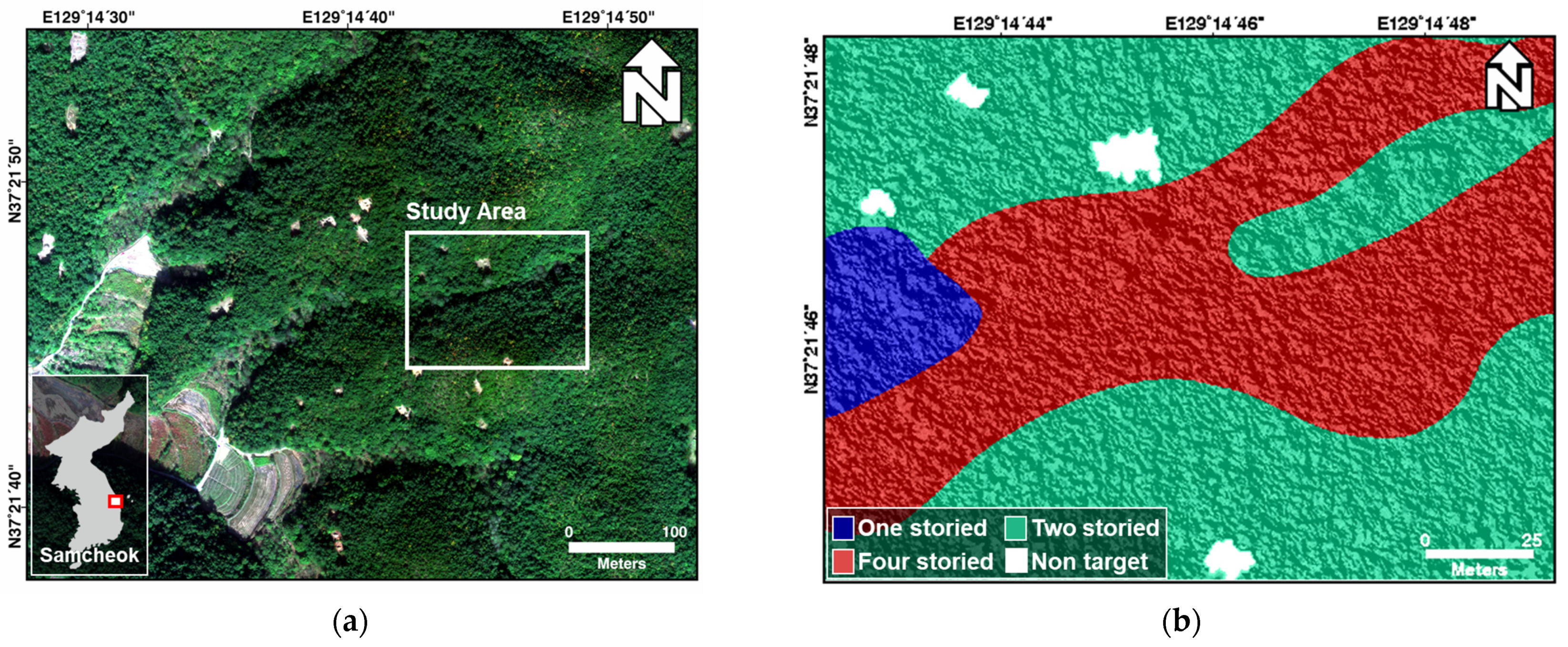
Figure 1. (a) Study area (Samcheok) and (b) ground truth (forest vertical structure) of this study.
Remotesensing 15 02833 g001
Figure 2. Data processing overall workflow.
Remotesensing 15 02833 g002
Figure 3. Modified U-Net architecture: (a) Model 1: a model with only a modified decoder structure; (b) Model 2: a model with modified encoder and decoder structures; and (c) Model 3: a model with modified encoder and decoder architecture, in addition to their connection.
Remotesensing 15 02833 g003
Figure 4. Optic and LiDAR data used in the study: (a) true color (R, G, B) composite image, (b) false color (red edge, NIR, B) composite image, and (c) LiDAR DSM acquired in October; (d) true color (R, G, B) composite image, (e) false color (red edge, NIR, B) composite image, and (f) LiDAR DSM acquired in November; (g) DTM provided by NGII.
Remotesensing 15 02833 g004aRemotesensing 15 02833 g004b
Figure 5. (a,b) Normalized NDVI and (c,d) SIPI index map calculated with October and November data, respectively; (e,f) normalized median and (g,h) standard deviation filtered canopy height map extracted from UAV LiDAR data acquired in October and November, respectively.
Remotesensing 15 02833 g005aRemotesensing 15 02833 g005b
Figure 6. Classification result of the forest vertical structure: (a) model with a modified decoder; (b) model with modified encoder and decoder; and (c) model with modified encoder and decoder, in addition to their connection; Box A represented the boundary of one- and four-storied, and Box B represented the boundary of two- and four-storied.
Remotesensing 15 02833 g006
Figure 7. Precision-recall curves derived from Models 1, 2, and 3. (a) the precision-recall curves in model 1; (b) the precision-recall curves in model 2; (c) the precision-recall curves in model 3. The blue lines represent the micro-average of the PR curve, and the purple, green, and red lines represent one-, two-, and four-storied curves, respectively.
Remotesensing 15 02833 g007
Table 1. Band characteristics of optic images acquired from an RX02 camera.
BandCenterWidth
Blue475 nm32 nm
Green560 nm27 nm
Red668 nm16 nm
Red Edge717 nm12 nm
Near infrared842 nm57 nm
Table 2. Specification of LiDAR sensor mounted on a UAV.
ParameterValue
Channels16 lasers
RangeUp to 200 m
Accuracy±3 cm
Field of View360° (H) × 30° (V)
Table 3. Spectral indices formulas that were used in this study.
NameFormula
NDVI N D V I = N I R R E D N I R + R E D
GNDVI G N D V I = N I R G R E E N N I R + G R E E N  
NDRE N D R E = N I R R E D   E d g e N I R + R E D   E d g e
SIPI S I P I = N I R B L U E N I R R E D
Table 4. Values of the correlation coefficient between spectral indices.
GNDVINDVINDRESIPI
GNDVI-0.8250.492−0.29
NDVI0.825-0.34−0.27
NDRE0.4920.34-−0.67
SIPI−0.29−0.27−0.67-
Table 5. Precision, recall, and F1-score based on the test result from Models 1,2 and 3.
ValueOne-StoriedTwo-StoriedFour-StoriedTotal
Model 1Precision0.9830.9850.9550.974
Recall0.9810.9610.9820.975
F1-score0.9820.9730.9680.974
Model 2Precision0.8670.9750.9380.927
Recall0.9910.9340.9670.964
F1-score0.9250.9540.9520.944
Model 3Precision0.7410.9620.9260.877
Recall0.9920.9110.9460.950
F1-score0.8480.9360.9360.907
Disclaimer/Publisher’s Note: The statements, opinions and data contained in all publications are solely those of the individual author(s) and contributor(s) and not of MDPI and/or the editor(s). MDPI and/or the editor(s) disclaim responsibility for any injury to people or property resulting from any ideas, methods, instructions or products referred to in the content.