
Machine Learning-Based Modeling of Air Temperature in the Complex Environment of Yerevan City, Armenia
 , ,
, ,
Abstract
1. Introduction
- Considering the complexity of the terrain configuration in Yerevan, to assess for the first time the feasibility of estimating urban Tair based on remote sensing data alone.
- Estimate the Urban Tair of the city of Yerevan using the PLSR model with a high (30) number of input variables.
2. Materials and Methods
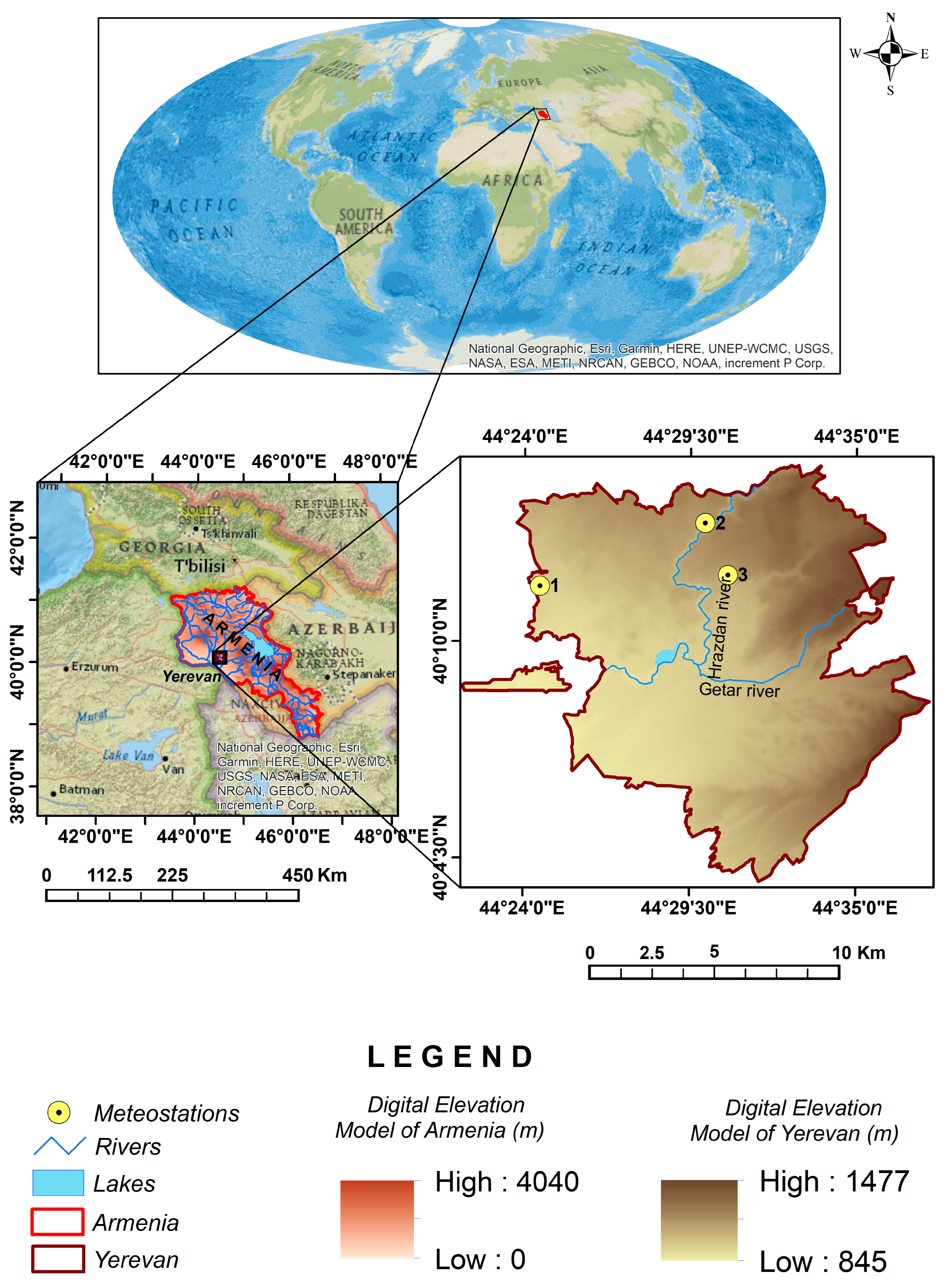
2.1. Test Site, Description and Terrain/Climate Features
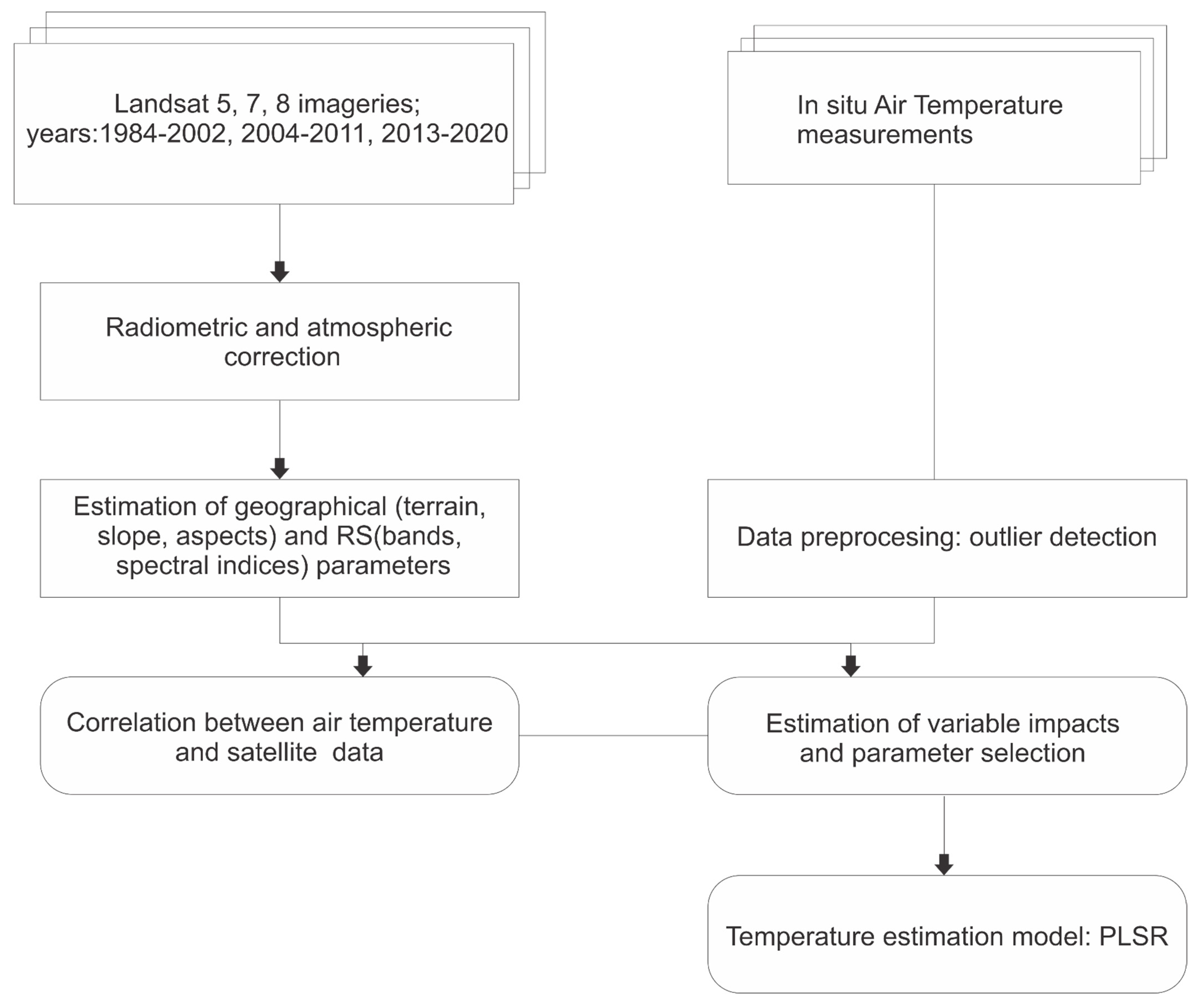
2.2. Preparation of Input Data
2.2.1. Satellite Data
2.2.2. Weather Data
3. Statistical Analysis and Modeling
4. Results and Discussions
5. Conclusions
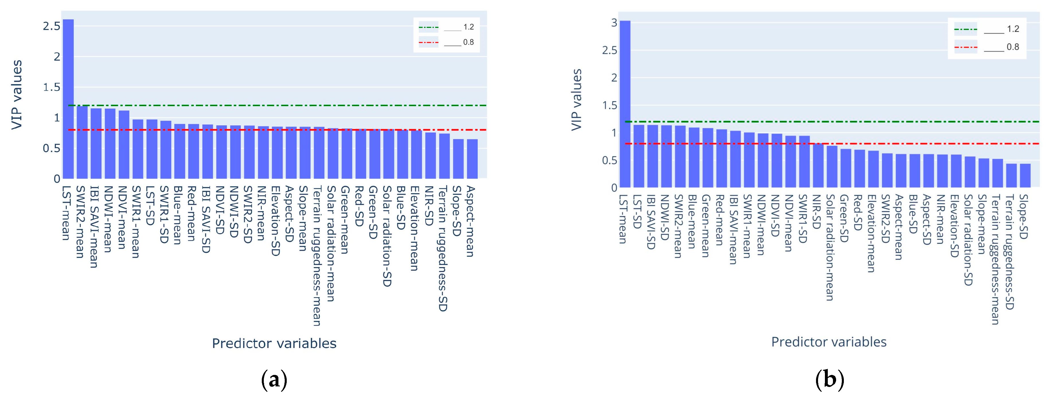
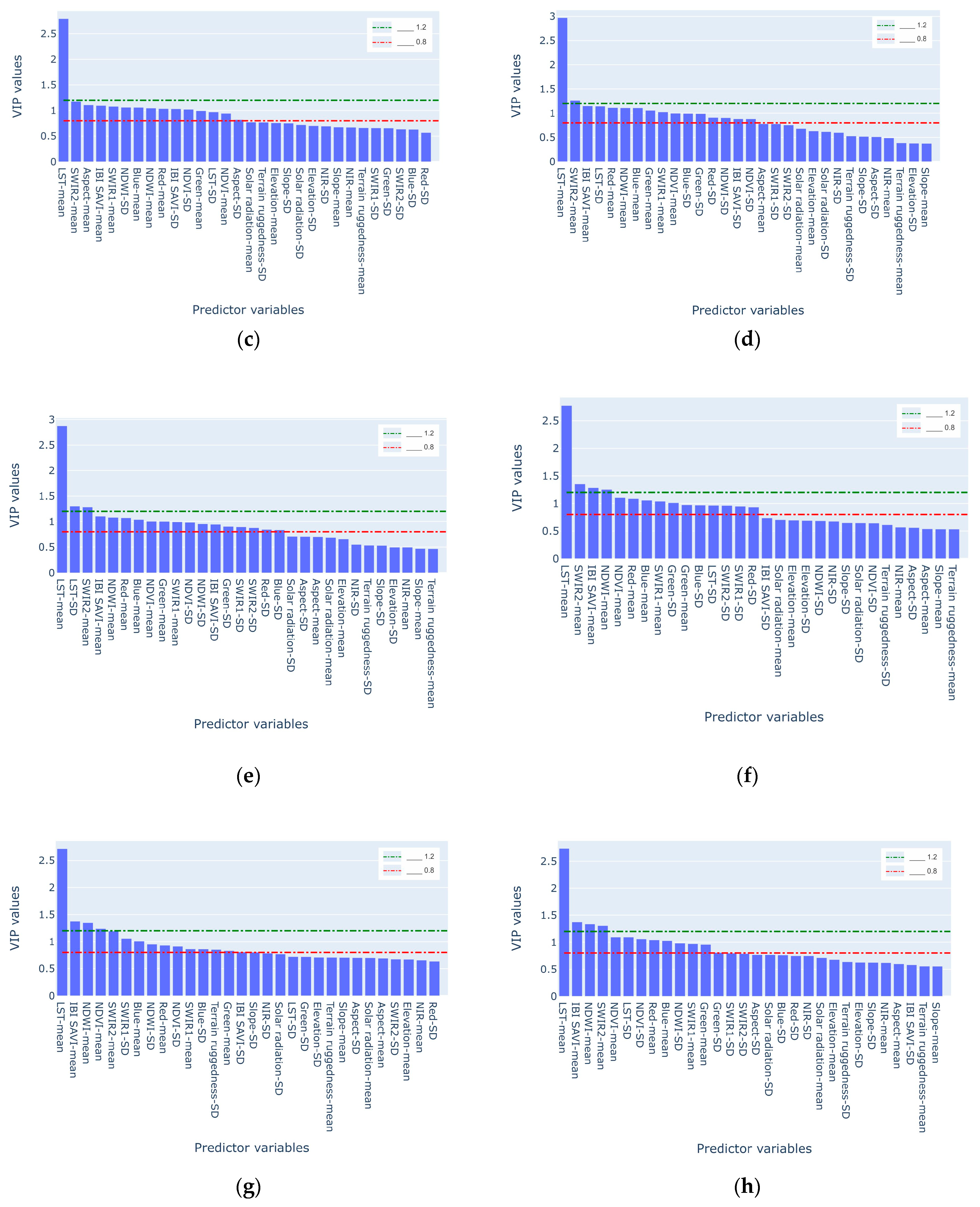
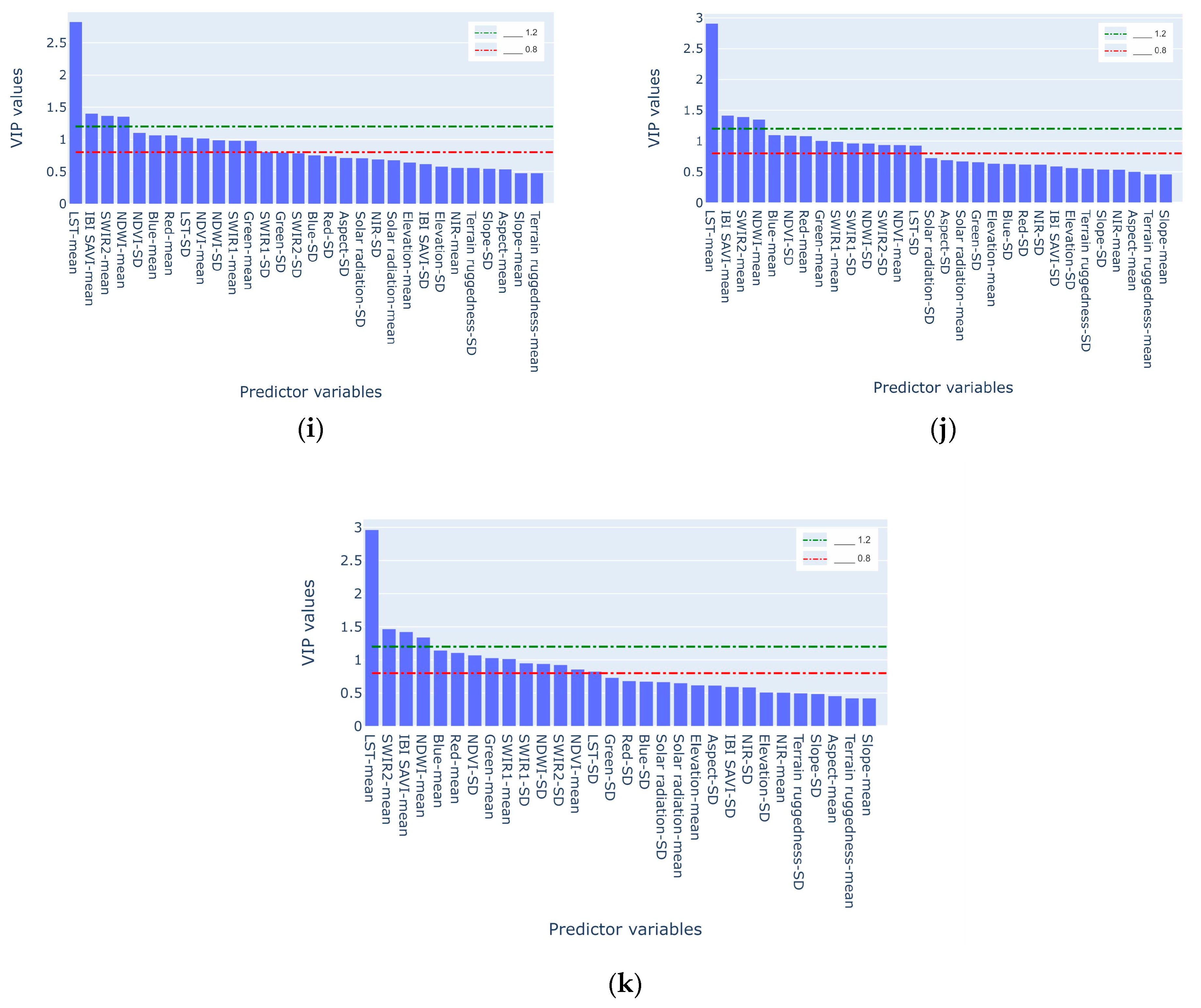
- Of the 30 parameters considered, 10 can be identified as relevant and can be used alone in the prediction; adding more parameters will not improve prediction, but will require more computational resources.
- The relevant parameters include a newly proposed modification of index IBI-SAVI, which turned out to strongly impact Tair prediction.
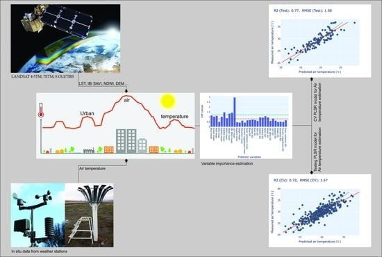
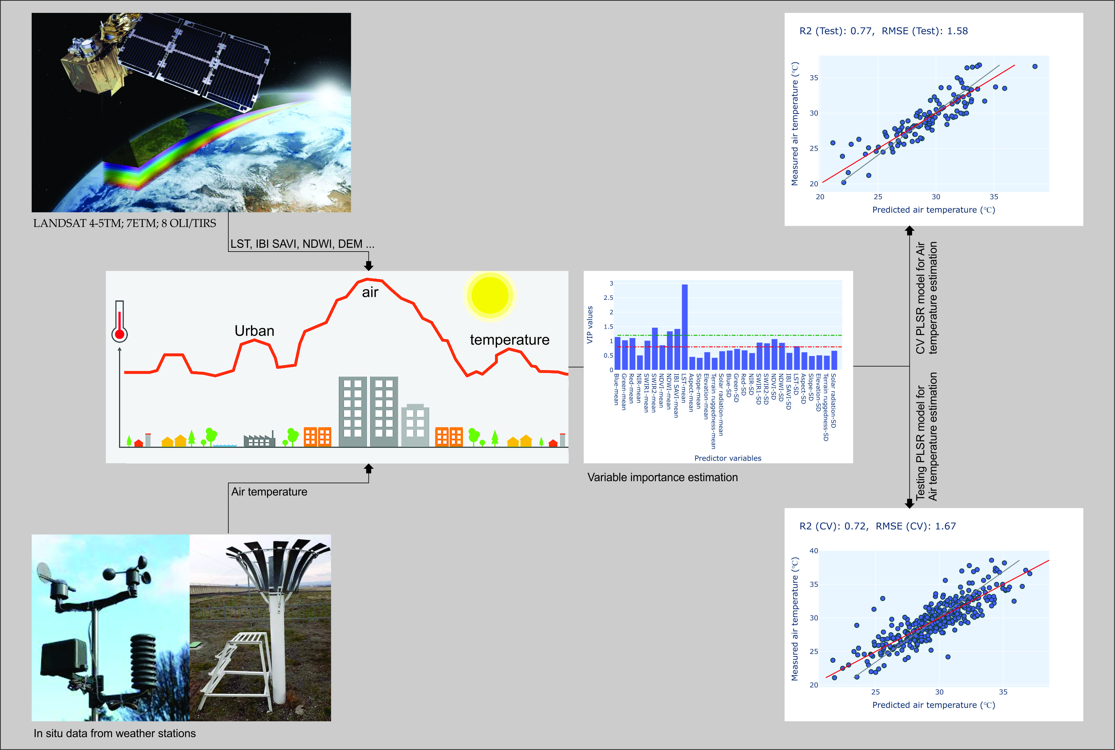
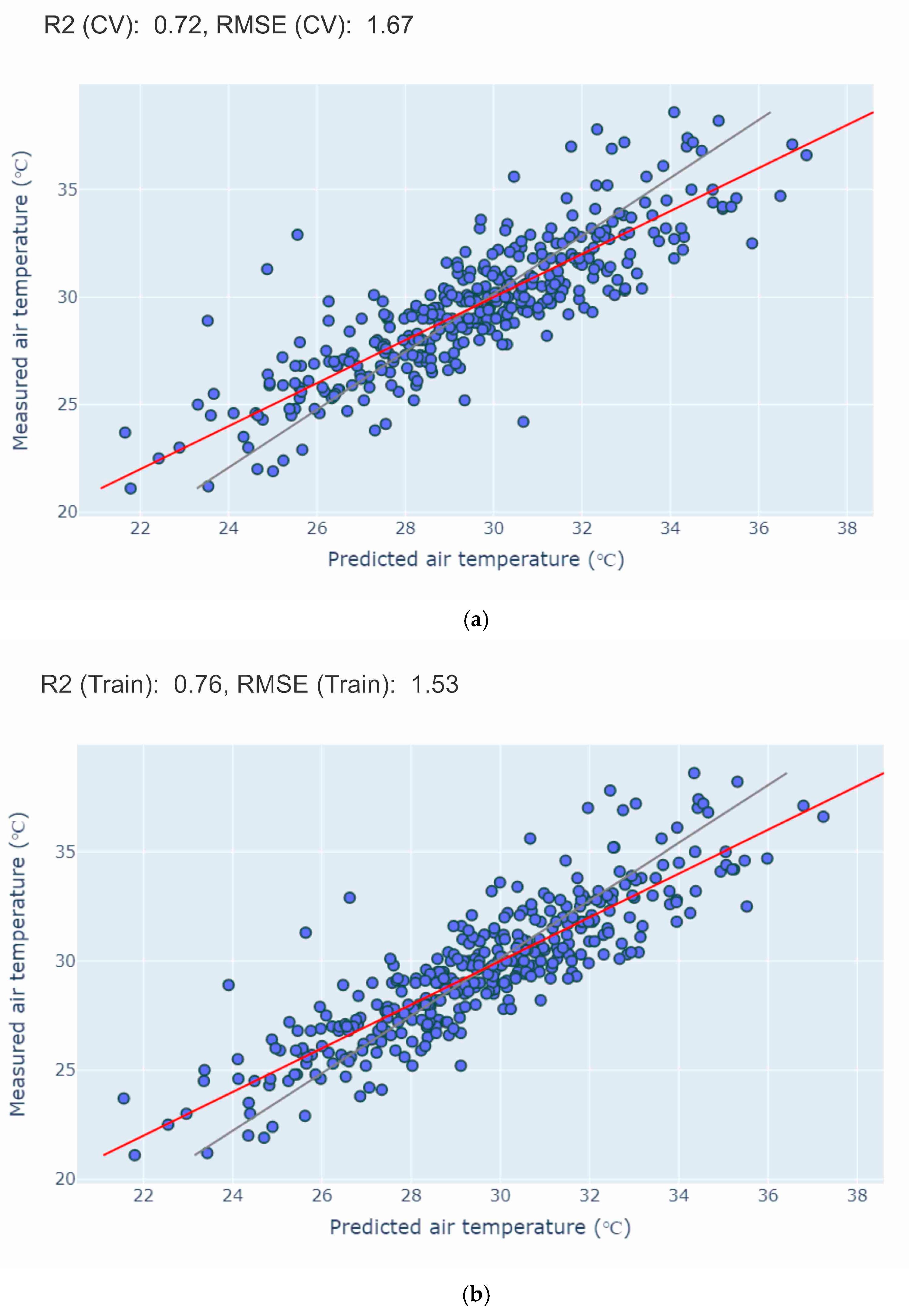
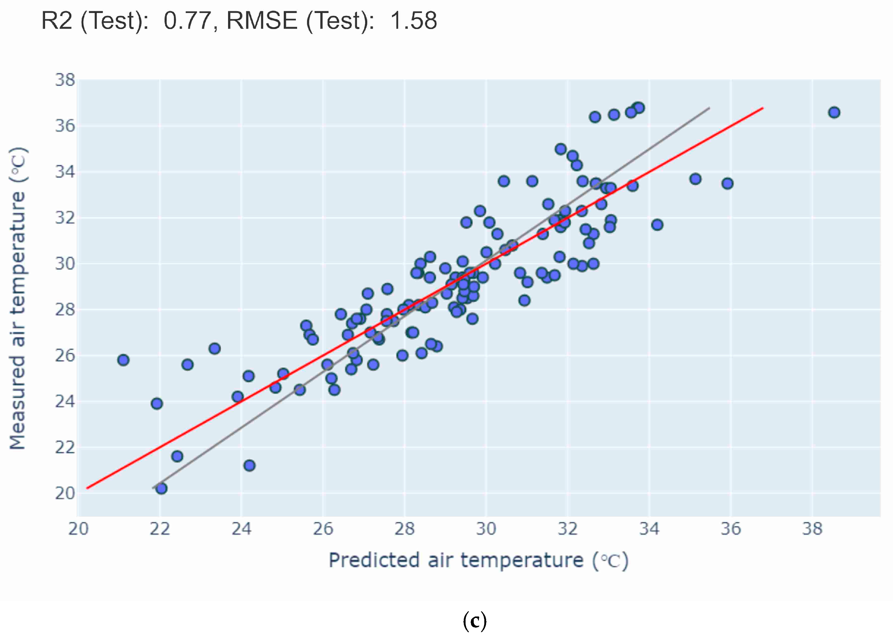
- Cross-validation analysis on temperature predictions across a station-centered 1000 m circular area revealed quite a high correlation (R2Val = 0.77, RMSEVal = 1.58) between the predicted and measured Tair from the test set.
- In light of the above, we may estimate that remote sensing is an effective tool to estimate Tair distribution where a dense network of weather stations is not available.
Author Contributions
Funding
Data Availability Statement
Acknowledgments
Conflicts of Interest
References
- Meliho, M.; Khattabi, A.; Zejli, D.; Orlando, C.A.; Dansou, C.E. Artificial Intelligence and Remote Sensing for Spatial Prediction of Daily Air Temperature: Case Study of Souss Watershed of Morocco. Geo-Spat. Inf. Sci. 2022, 25, 244–258. [Google Scholar] [CrossRef]
- Ding, L.; Zhou, J.; Zhang, X.; Liu, S.; Cao, R. Downscaling of Surface Air Temperature over the Tibetan Plateau Based on DEM. Int. J. Appl. Earth Obs. Geoinf. 2018, 73, 136–147. [Google Scholar] [CrossRef]
- Shah, D.B.; Pandya, M.R.; Trivedi, H.J.; Jani, A.R. Estimating Minimum and Maximum Air Temperature Using MODIS Data over Indo-Gangetic Plain. J. Earth Syst. Sci. 2013, 122, 1593–1605. [Google Scholar] [CrossRef]
- Nichol, J.E.; To, P.H. Temporal Characteristics of Thermal Satellite Images for Urban Heat Stress and Heat Island Mapping. ISPRS J. Photogramm. Remote Sens. 2012, 74, 153–162. [Google Scholar] [CrossRef]
- Fu, P.; Weng, Q. Variability in Annual Temperature Cycle in the Urban Areas of the United States as Revealed by MODIS Imagery. ISPRS J. Photogramm. Remote Sens. 2018, 146, 65–73. [Google Scholar] [CrossRef]
- Vogt, J.V.; Viau, A.A.; Paquet, F. Mapping Regional Air Temperature Fields Using Satellite-Derived Surface Skin Temperatures. Int. J. Climatol. 1997, 17, 1559–1579. [Google Scholar] [CrossRef]
- Zakšek, K.; Schroedter-Homscheidt, M. Parameterization of Air Temperature in High Temporal and Spatial Resolution from a Combination of the SEVIRI and MODIS Instruments. ISPRS J. Photogramm. Remote Sens. 2009, 64, 414–421. [Google Scholar] [CrossRef]
- Cristóbal, J.; Ninyerola, M.; Pons, X. Modeling Air Temperature through a Combination of Remote Sensing and GIS Data. J. Geophys. Res. 2008, 113, D13106. [Google Scholar] [CrossRef]
- Mutiibwa, D.; Strachan, S.; Albright, T. Land Surface Temperature and Surface Air Temperature in Complex Terrain. IEEE J. Sel. Top. Appl. Earth Obs. Remote Sens. 2015, 8, 4762–4774. [Google Scholar] [CrossRef]
- Nikoloudakis, N.; Stagakis, S.; Mitraka, Z.; Kamarianakis, Y.; Chrysoulakis, N. Spatial Interpolation of Urban Air Temperatures Using Satellite-Derived Predictors. Appl. Clim. 2020, 141, 657–672. [Google Scholar] [CrossRef]
- Orellana-Samaniego, M.L.; Ballari, D.; Guzman, P.; Ospina, J.E. Estimating Monthly Air Temperature Using Remote Sensing on a Region with Highly Variable Topography and Scarce Monitoring in the Southern Ecuadorian Andes. Appl Clim. 2021, 144, 949–966. [Google Scholar] [CrossRef]
- Yoo, C.; Im, J.; Park, S.; Quackenbush, L.J. Estimation of Daily Maximum and Minimum Air Temperatures in Urban Landscapes Using MODIS Time Series Satellite Data. ISPRS J. Photogramm. Remote Sens. 2018, 137, 149–162. [Google Scholar] [CrossRef]
- Cifuentes, J.; Marulanda, G.; Bello, A.; Reneses, J. Air Temperature Forecasting Using Machine Learning Techniques: A Review. Energies 2020, 13, 4215. [Google Scholar] [CrossRef]
- Bechtel, B.; Zakšek, K.; Oßenbrügge, J.; Kaveckis, G.; Böhner, J. Towards a Satellite Based Monitoring of Urban Air Temperatures. Sustain. Cities Soc. 2017, 34, 22–31. [Google Scholar] [CrossRef]
- Ho, H.C.; Knudby, A.; Sirovyak, P.; Xu, Y.; Hodul, M.; Henderson, S.B. Mapping Maximum Urban Air Temperature on Hot Summer Days. Remote Sens. Environ. 2014, 154, 38–45. [Google Scholar] [CrossRef]
- Agathangelidis, I.; Cartalis, C.; Santamouris, M. Estimation of Air Temperatures for the Urban Agglomeration of Athens with the Use of Satellite Data. Geoinform. Geostat. Overv. 2016, 4, 1–7. [Google Scholar] [CrossRef]
- Ho, H.C.; Knudby, A.; Xu, Y.; Hodul, M.; Aminipouri, M. A Comparison of Urban Heat Islands Mapped Using Skin Temperature, Air Temperature, and Apparent Temperature (Humidex), for the Greater Vancouver Area. Sci. Total Environ. 2016, 544, 929–938. [Google Scholar] [CrossRef]
- Meyer, H.; Pebesma, E. Predicting into Unknown Space? Estimating the Area of Applicability of Spatial Prediction Models. Methods Ecol. Evol. 2021, 12, 1620–1633. [Google Scholar] [CrossRef]
- Xu, Y.; Shen, Y. Reconstruction of the Land Surface Temperature Time Series Using Harmonic Analysis. Comput. Geosci. 2013, 61, 126–132. [Google Scholar] [CrossRef]
- Noi, P.T.; Degener, J.; Kappas, M. Comparison of Multiple Linear Regression, Cubist Regression, and Random Forest Algorithms to Estimate Daily Air Surface Temperature from Dynamic Combinations of MODIS LST Data. Remote Sens. 2017, 9, 398. [Google Scholar] [CrossRef]
- Otgonbayar, M.; Atzberger, C.; Mattiuzzi, M.; Erdenedalai, A. Estimation of Climatologies of Average Monthly Air Temperature over Mongolia Using MODIS Land Surface Temperature (LST) Time Series and Machine Learning Techniques. Remote Sens. 2019, 11, 2588. [Google Scholar] [CrossRef]
- Wang, C.; Bi, X.; Luan, Q.; Li, Z. Estimation of Daily and Instantaneous Near-Surface Air Temperature from MODIS Data Using Machine Learning Methods in the Jingjinji Area of China. Remote Sens. 2022, 14, 1916. [Google Scholar] [CrossRef]
- Rasul, A.; Balzter, H.; Smith, C. Applying a Normalized Ratio Scale Technique to Assess Influences of Urban Expansion on Land Surface Temperature of the Semi-Arid City of Erbil. Int. J. Remote Sens. 2017, 38, 3960–3980. [Google Scholar] [CrossRef]
- Statistical Committee of the Republic of Armenia. Available online: https://www.armstat.am/en/ (accessed on 13 March 2023).
- Yerevan Green City Action Plan. Available online: https://www.yerevan.am/en/yerevan-green-city-action-plan/ (accessed on 13 March 2023).
- Tepanosyan, G.; Muradyan, V.; Hovsepyan, A.; Pinigin, G.; Medvedev, A.; Asmaryan, S. Studying Spatial-Temporal Changes and Relationship of Land Cover and Surface Urban Heat Island Derived through Remote Sensing in Yerevan, Armenia. Build. Environ. 2021, 187, 107390. [Google Scholar] [CrossRef]
- Climate Change Information Center. Available online: http://www.nature-ic.am/en (accessed on 13 March 2023).
- Third National Communication on Climate Change: Under the United Nations Framework Convention on Climate Change; “Lusabats” Publishing House, Yerevan, 2015. Available online: https://unfccc.int/resource/docs/natc/armnc3.pdf (accessed on 13 March 2023).
- Foga, S.; Scaramuzza, P.L.; Guo, S.; Zhu, Z.; Dilley, R.D.; Beckmann, T.; Schmidt, G.L.; Dwyer, J.L.; Joseph Hughes, M.; Laue, B. Cloud Detection Algorithm Comparison and Validation for Operational Landsat Data Products. Remote Sens. Environ. 2017, 194, 379–390. [Google Scholar] [CrossRef]
- Xu, H. A New Index for Delineating Built-up Land Features in Satellite Imagery. Int. J. Remote Sens. 2008, 29, 4269–4276. [Google Scholar] [CrossRef]
- Parastatidis, D.; Mitraka, Z.; Chrysoulakis, N.; Abrams, M. Online Global Land Surface Temperature Estimation from Landsat. Remote Sens. 2017, 9, 1208. [Google Scholar] [CrossRef]
- Jimenez-Munoz, J.C.; Cristobal, J.; Sobrino, J.A.; Soria, G.; Ninyerola, M.; Pons, X.; Pons, X. Revision of the Single-Channel Algorithm for Land Surface Temperature Retrieval from Landsat Thermal-Infrared Data. IEEE Trans. Geosci. Remote Sens. 2009, 47, 339–349. [Google Scholar] [CrossRef]
- Jimenez-Munoz, J.C.; Sobrino, J.A.; Skokovic, D.; Mattar, C.; Cristobal, J. Land Surface Temperature Retrieval Methods From Landsat-8 Thermal Infrared Sensor Data. IEEE Geosci. Remote Sens. Lett. 2014, 11, 1840–1843. [Google Scholar] [CrossRef]
- Riley, S.; Degloria, S.; Elliot, S.D. A Terrain Ruggedness Index That Quantifies Topographic Heterogeneity. Int. J. Sci. 1999, 5, 23–27. [Google Scholar]
- Chuai, X.W.; Huang, X.J.; Wang, W.J.; Bao, G. NDVI, Temperature and Precipitation Changes and Their Relationships with Different Vegetation Types during 1998–2007 in Inner Mongolia, China. Int. J. Climatol. 2013, 33, 1696–1706. [Google Scholar] [CrossRef]
- Hou, G.; Zhang, H.; Wang, Y. Vegetation Dynamics and Its Relationship with Climatic Factors in the Changbai Mountain Natural Reserve. J. Mt. Sci. 2011, 8, 865–875. [Google Scholar] [CrossRef]
- Yagoub, Y.E.; Li, Z.; Musa, O.S.; Anjum, M.N.; Wang, F.; Bi, Y.; Zhang, B. Correlation between Climate Factors and Vegetation Cover in Qinghai Province, China. J. Geogr. Inf. Syst. 2017, 9, 403–419. [Google Scholar] [CrossRef]
- Zhao, Z.-Q.; He, B.-J.; Li, L.-G.; Wang, H.-B.; Darko, A. Profile and Concentric Zonal Analysis of Relationships between Land Use/Land Cover and Land Surface Temperature: Case Study of Shenyang, China. Energy Build. 2017, 155, 282–295. [Google Scholar] [CrossRef]
- Cui, L.; Shi, J. Temporal and Spatial Response of Vegetation NDVI to Temperature and Precipitation in Eastern China. J. Geogr. Sci. 2010, 20, 163–176. [Google Scholar] [CrossRef]
- Gitelson, A.A.; Kaufman, Y.J. MODIS NDVI optimization to fit the AVHRR data series—Spectral considerations. Remote Sens. Environ. 1998, 66, 343–350. [Google Scholar] [CrossRef]
- Pedregosa, F.; Varoquaux, G.; Gramfort, A.; Michel, V.; Thirion, B.; Grisel, O.; Blondel, M.; Prettenhofer, P.; Weiss, R.; Dubourg, V.; et al. Scikit-Learn: Machine Learning in Python. J. Mach. Learn. Res. 2012, 12, 2825–2830. [Google Scholar]
- Zakharov, V.P.; Bratchenko, I.A.; Artemyev, D.N.; Myakinin, O.O.; Kozlov, S.V.; Moryatov, A.A.; Orlov, A.E. 17-Multimodal Optical Biopsy and Imaging of Skin Cancer. In Neurophotonics and Biomedical Spectroscopy; Elsevier: Amsterdam, The Netherlands, 2019; pp. 449–476. ISBN 978-0-323-48067-3. [Google Scholar]
- Benali, A.; Carvalho, A.C.; Nunes, J.P.; Carvalhais, N.; Santos, A. Estimating Air Surface Temperature in Portugal Using MODIS LST Data. Remote Sens. Environ. 2012, 124, 108–121. [Google Scholar] [CrossRef]
- Zhang, H.; Zhang, F.; Ye, M.; Che, T.; Zhang, G. Estimating Daily Air Temperatures over the Tibetan Plateau by Dynamically Integrating MODIS LST Data. JGR Atmos. 2016, 121, 11–425. [Google Scholar] [CrossRef]


| N | Name of Station | Latitude | Longitude | Height a. s. l. (m) |
|---|---|---|---|---|
| 1. | Yerevan_agro | 40°11′19″N | 44°23′55″E | 942 |
| 2. | Yerevan_aerologia | 40°13′2″N | 44°29′59″E | 1134 |
| 3. | Arabkir | 40°11′43″N | 44°30′44″E | 1113 |
| N | Variables | Correlation Coefficient (r) | p_Value |
|---|---|---|---|
| 1. | Blue_mean | 0.14 | 2 × 10⁻³ |
| 2. | Green_mean | 0.16 | 4 × 10⁻⁴ |
| 3. | Red_mean | 0.26 | 3 × 10⁻⁹ |
| 4. | NIR_mean | 0.01 | 8 × 10⁻¹ |
| 5. | SWIR1_mean | 0.29 | 7 × 10⁻¹¹ |
| 6. | SWIR2_mean | 0.30 | 9 × 10⁻¹² |
| 7. | NDVI_mean | −0.25 | 1 × 10⁻⁸ |
| 8. | NDWI_mean | −0.35 | 2 × 10⁻¹⁵ |
| 9. | IBI SAVI_mean | 0.35 | 1 × 10⁻¹⁵ |
| 10. | LST_mean | 0.79 | 1 × 10⁻¹⁵ |
| 11. | Aspect_mean | −0.07 | 1 × 10⁻¹ |
| 12. | Slope_mean | −0.06 | 2 × 10⁻¹ |
| 13. | Elev_mean | −0.08 | 7 × 10⁻² |
| 14. | Rugged_mean | −0.06 | 2 × 10⁻¹ |
| 15. | Sol_rad_mean | −0.19 | 1 × 10⁻⁵ |
| 16. | Blue_SD | −0.10 | 3 × 10⁻² |
| 17. | Green_SD | −0.09 | 4 × 10⁻² |
| 18. | Red_SD | −0.07 | 1 × 10⁻¹ |
| 19. | NIR_SD | −0.07 | 1 × 10⁻¹ |
| 20. | SWIR1_SD | −0.09 | 4 × 10⁻² |
| 21. | SWIR2_SD | −0.13 | 3 × 10⁻³ |
| 22. | NDVI_SD | −0.26 | 2 × 10⁻⁹ |
| 23. | NDWI_SD | −0.24 | 5 × 10⁻⁸ |
| 24. | IBI SAVI_SD | −0.12 | 5 × 10⁻³ |
| 25. | LST_SD | −0.01 | 9 × 10⁻¹ |
| 26. | Aspect_SD | 0.11 | 1 × 10⁻² |
| 27. | Slope_SD | −0.03 | 6 × 10⁻¹ |
| 28. | Elev_SD | −0.10 | 3 × 10⁻² |
| 29. | Rugged_SD | −0.02 | 6 × 10⁻¹ |
| 30. | Sol_rad_SD | 0.04 | 4 × 10⁻¹ |
| PLSR Descriptive | 30 m | 100 m | 200 m | 300 m | 400 m | 500 m | 600 m | 700 m | 800 m | 900 m | 1000 m |
|---|---|---|---|---|---|---|---|---|---|---|---|
| R2Train | 0.72 | 0.73 | 0.73 | 0.75 | 0.75 | 0.74 | 0.75 | 0.75 | 0.75 | 0.76 | 0.76 |
| RMSETrain | 1.68 | 1.66 | 1.65 | 1.58 | 1.58 | 1.61 | 1.60 | 1.59 | 1.59 | 1.57 | 1.56 |
| R2CV | 0.68 | 0.68 | 0.68 | 0.71 | 0.71 | 0.70 | 0.71 | 0.70 | 0.70 | 0.71 | 0.72 |
| RMSECV | 1.80 | 1.79 | 1.80 | 1.70 | 1.70 | 1.73 | 1.73 | 1.74 | 1.74 | 1.71 | 1.67 |
| R2Test | 0.70 | 0.71 | 0.71 | 0.73 | 0.72 | 0.73 | 0.72 | 0.74 | 0.74 | 0.75 | 0.77 |
| RMSETest | 1.78 | 1.73 | 1.75 | 1.69 | 1.71 | 1.69 | 1.72 | 1.65 | 1.65 | 1.61 | 1.58 |
| N of VIP components | 14 | 14 | 10 | 14 | 14 | 13 | 14 | 10 | 10 | 10 | 10 |
| N | Predictor Variables | VIP Scores |
|---|---|---|
| 1. | Blue-mean | 1.113 |
| 2. | Green-mean | 1.019 |
| 3. | Red-mean | 1.098 |
| 4. | NIR-mean | 0.683 |
| 5. | SWIR1-mean | 1.067 |
| 6. | SWIR2-mean | 1.415 |
| 7. | NDVI-mean | 0.8985 |
| 8. | NDWI-mean | 1.225 |
| 9. | IBI SAVI-mean | 1.285 |
| 10. | LST-mean | 2.772 |
| 11. | Aspect-mean | 0.661 |
| 12. | Slope-mean | 0.667 |
| 13. | Elevation-mean | 0.643 |
| 14. | Terrain ruggedness-mean | 0.666 |
| 15. | Solar radiation-mean | 0.661 |
| 16. | Blue-SD | 0.730 |
| 17. | Green-SD | 0.692 |
| 18. | Red-SD | 0.658 |
| 19. | NIR-SD | 0.712 |
| 20. | SWIR1-SD | 0.910 |
| 21. | SWIR2-SD | 0.894 |
| 22. | NDVI-SD | 1.011 |
| 23. | NDWI-SD | 0.923 |
| 24. | IBI SAVI-SD | 0.586 |
| 25. | LST-SD | 0.960 |
| 26. | Aspect-SD | 0.746 |
| 27. | Slope-SD | 0.651 |
| 28. | Elevation-SD | 0.710 |
| 29. | Terrain ruggedness-SD | 0.650 |
| 30. | Solar radiation-SD | 0.688 |
Disclaimer/Publisher’s Note: The statements, opinions and data contained in all publications are solely those of the individual author(s) and contributor(s) and not of MDPI and/or the editor(s). MDPI and/or the editor(s) disclaim responsibility for any injury to people or property resulting from any ideas, methods, instructions or products referred to in the content. |
© 2023 by the authors. Licensee MDPI, Basel, Switzerland. This article is an open access article distributed under the terms and conditions of the Creative Commons Attribution (CC BY) license (https://creativecommons.org/licenses/by/4.0/).
Share and Cite
Tepanosyan, G.; Asmaryan, S.; Muradyan, V.; Avetisyan, R.; Hovsepyan, A.; Khlghatyan, A.; Ayvazyan, G.; Dell’Acqua, F. Machine Learning-Based Modeling of Air Temperature in the Complex Environment of Yerevan City, Armenia. Remote Sens. 2023, 15, 2795. https://doi.org/10.3390/rs15112795
Tepanosyan G, Asmaryan S, Muradyan V, Avetisyan R, Hovsepyan A, Khlghatyan A, Ayvazyan G, Dell’Acqua F. Machine Learning-Based Modeling of Air Temperature in the Complex Environment of Yerevan City, Armenia. Remote Sensing. 2023; 15(11):2795. https://doi.org/10.3390/rs15112795
Chicago/Turabian StyleTepanosyan, Garegin, Shushanik Asmaryan, Vahagn Muradyan, Rima Avetisyan, Azatuhi Hovsepyan, Anahit Khlghatyan, Grigor Ayvazyan, and Fabio Dell’Acqua. 2023. "Machine Learning-Based Modeling of Air Temperature in the Complex Environment of Yerevan City, Armenia" Remote Sensing 15, no. 11: 2795. https://doi.org/10.3390/rs15112795
APA StyleTepanosyan, G., Asmaryan, S., Muradyan, V., Avetisyan, R., Hovsepyan, A., Khlghatyan, A., Ayvazyan, G., & Dell’Acqua, F. (2023). Machine Learning-Based Modeling of Air Temperature in the Complex Environment of Yerevan City, Armenia. Remote Sensing, 15(11), 2795. https://doi.org/10.3390/rs15112795