Article

Assessment of Wildfire Susceptibility and Wildfire Threats to Ecological Environment and Urban Development Based on GIS and Multi-Source Data: A Case Study of Guilin, China

1
College of Geomatics and Geoinformation, Guilin University of Technology, 319 Yanshan Street, Guilin 541006, China
2
Guangxi Key Laboratory of Spatial Information and Geomatics, 319 Yanshan Street, Guilin 541006, China
*
Author to whom correspondence should be addressed.
Remote Sens. 2023, 15(10), 2659; https://doi.org/10.3390/rs15102659
Submission received: 27 April 2023 / Revised: 16 May 2023 / Accepted: 18 May 2023 / Published: 19 May 2023
(This article belongs to the Special Issue Artificial Intelligence for Natural Hazards (AI4NH))

Abstract

:
The frequent occurrence and spread of wildfires pose a serious threat to the ecological environment and urban development. Therefore, assessing regional wildfire susceptibility is crucial for the early prevention of wildfires and formulation of disaster management decisions. However, current research on wildfire susceptibility primarily focuses on improving the accuracy of models, while lacking in-depth study of the causes and mechanisms of wildfires, as well as the impact and losses they cause to the ecological environment and urban development. This situation not only increases the uncertainty of model predictions but also greatly reduces the specificity and practical significance of the models. We propose a comprehensive evaluation framework to analyze the spatial distribution of wildfire susceptibility and the effects of influencing factors, while assessing the risks of wildfire damage to the local ecological environment and urban development. In this study, we used wildfire information from the period 2013–2022 and data from 17 susceptibility factors in the city of Guilin as the basis, and utilized eight machine learning algorithms, namely logistic regression (LR), artificial neural network (ANN), K-nearest neighbor (KNN), support vector regression (SVR), random forest (RF), gradient boosting decision tree (GBDT), light gradient boosting machine (LGBM), and eXtreme gradient boosting (XGBoost), to assess wildfire susceptibility. By evaluating multiple indicators, we obtained the optimal model and used the Shapley Additive Explanations (SHAP) method to explain the effects of the factors and the decision-making mechanism of the model. In addition, we collected and calculated corresponding indicators, with the Remote Sensing Ecological Index (RSEI) representing ecological vulnerability and the Night-Time Lights Index (NTLI) representing urban development vulnerability. The coupling results of the two represent the comprehensive vulnerability of the ecology and city. Finally, by integrating wildfire susceptibility and vulnerability information, we assessed the risk of wildfire disasters in Guilin to reveal the overall distribution characteristics of wildfire disaster risk in Guilin. The results show that the AUC values of the eight models range from 0.809 to 0.927, with accuracy values ranging from 0.735 to 0.863 and RMSE values ranging from 0.327 to 0.423. Taking into account all the performance indicators, the XGBoost model provides the best results, with AUC, accuracy, and RMSE values of 0.927, 0.863, and 0.327, respectively. This indicates that the XGBoost model has the best predictive performance. The high-susceptibility areas are located in the central, northeast, south, and southwest regions of the study area. The factors of temperature, soil type, land use, distance to roads, and slope have the most significant impact on wildfire susceptibility. Based on the results of the ecological vulnerability and urban development vulnerability assessments, potential wildfire risk areas can be identified and assessed comprehensively and reasonably. The research results of this article not only can improve the specificity and practical significance of wildfire prediction models but also provide important reference for the prevention and response of wildfires.

1. Introduction

Wildfire disasters refer to unplanned and uncontrolled fires that occur in natural environments such as forests, farmland, grasslands, and areas around human settlements [1]. Wildfires not only lead to the loss of natural resources such as forests and grasslands, resulting in a reduction of biodiversity, but also cause damage to soil texture, water resources, and surface environments. They pose a threat to the lives and property of the general public, and directly or indirectly cause economic losses to local industries such as agriculture and tourism [2]. Due to the significant impact of wildfires on ecosystems and socio-economic development, the prediction and management of wildfire disasters have become the main focus of governments and the global scientific community [3]. Wildfires have become more frequent in recent years in various regions of China, especially Guangxi, due to the increased incidence of extreme weather conditions such as high temperatures and droughts, along with the accelerated process of urbanization resulting in deforestation and land development [4]. Therefore, as an important component of wildfire monitoring and prediction, government departments and industries such as tourism and transportation can develop wildfire prevention plans and effectively avoid losses caused by wildfire disasters based on the results of wildfire susceptibility assessments.
Existing research indicates that the causes of wildfires are complex, involving various environmental and anthropogenic factors [5]. For instance, meteorological conditions, land use, topography, and human activities are all potential factors that may affect the probability and magnitude of wildland fire occurrence [6]. For example, in dry and hot environments, the combination of low vegetation coverage and strong winds may significantly increase the degree of wildfire susceptibility. In urban fringe areas, higher population density and human activities may more easily trigger wildland fires and accelerate their spread. Additionally, the weights and variables of the wildfire susceptibility modeling index may differ across different regions [7]. This is due to the variations in terrain, climate, ecology, and population between different areas, resulting in different impacts on wildfire occurrence. Therefore, to assess the susceptibility of wildland fires in a specific area, it is necessary to comprehensively consider the local natural environment, climate conditions, human activities, and attempt to identify the factors that have significant impacts on wildfire occurrence in that area.
With the continuous development of fields such as computer science, geographic information systems, and remote sensing technology, the research methods for regional wildfire susceptibility have undergone a process from qualitative analysis and semi-quantitative analysis to quantitative analysis. Qualitative and semi-quantitative analysis methods, such as expert scoring and hierarchical analysis, generally require rich expert experience as the judgment standard for whether a wildfire event occurs [8,9]. However, these methods rely on human prior knowledge, and when expert opinions are not correct, the calculation results will deviate from objective facts [10]. In contrast, quantitative analysis methods based on data-driven physical models, conditional probability models, and machine learning (ML) algorithms are more reasonable and accurate for evaluating the susceptibility of natural disasters such as wildfires. Among them, physical models are mainly based on fluid mechanics and heat transfer mechanisms, and the probability of wildfire occurrence is obtained by inputting detailed physical parameters. However, it is difficult to obtain data for such methods, and their applicability is limited [11]. Common conditional probability models include frequency ratio [12], evidential belief function [13], and weights of evidence [14]. Such models can explicitly reflect the connection between wildfires and different attribute intervals of a single conditioning factor through statistical algorithms, with simple calculations. However, they cannot accurately express the weight and correlation of each indicator factor, nor can they fully express the complex relationship between conditioning factors and wildfire events [15]. In recent years, various ML models such as logistic regression (LR) [16], artificial neural networks (ANN) [17], support vector machines (SVM) [18], random forests (RF) [19], and gradient boosting decision trees (GBDT) [20] have been widely applied in the evaluation of wildfire susceptibility. They establish a connection between wildfire data and different conditioning factors, and can better fit data samples and highlight the nonlinear relationship between wildfires and factors, thus achieving more accurate prediction results [21].
Currently, research on ML-based wildfire susceptibility has two main shortcomings. Firstly, research is mainly focused on upgrading algorithms and models to improve prediction accuracy, while lacking explanations on the relationship between factors and wildfire events. Although machine learning models have great advantages in dealing with nonlinear problems, they are essentially black box models that lack interpretability, and cannot comprehensively evaluate the prediction results of wildfire susceptibility [22,23]. Therefore, an objective and interpretable method is needed to identify key factors that affect wildfire disasters and clarify the decision mechanism of the model, helping wildfire risk prevention and control workers better understand the assessment results of wildfire susceptibility. SHapley Additive exPlanations (SHAP), based on the idea of game theory, is one of the latest interpretability methods that can solve this problem [24,25]. The SHAP algorithm provides two different interpretation methods: global and local explanations. Global interpretation analyzes the entire dataset to show the contribution of each input feature to the target variable across the dataset, thereby explaining the behavior and prediction results of the entire model. This method is useful in identifying overall trends and patterns but lacks detailed explanations for individual samples. Correspondingly, local interpretation can provide more detailed and specific information, and this method has been applied to local interpretation assessments of disasters such as landslides, floods, and earthquakes [26,27,28,29]. In wildfire susceptibility studies, local interpretation methods can help researchers better understand the impact of individual samples on overall wildfire susceptibility, thereby improving the interpretability and reliability of predictions. Additionally, it can reveal the importance of specific factors for specific samples, providing more specific and practical information to support wildfire management and prevention efforts.
Secondly, current research on regional wildfire disasters mainly focuses on wildfire susceptibility (the degree of spatial possibility of wildfire occurrence), while research on wildfire risk (the degree of risk of damage caused) is relatively scarce. The study of wildfire risk is aimed at improving disaster risk prevention capabilities to mitigate the threat of wildfire disasters to human life, property, and social development, making the prediction results of wildfire susceptibility meaningful [30]. Therefore, assessing only regional wildfire susceptibility is not enough, and the potential risk level of wildfire losses must also be analyzed [31]. Considering that wildfire risk assessment is a complex natural and social problem, it not only involves the loss caused by wildfires to the ecology but also affects the ecology and cities [32]. At the same time, studying only the ecological environment or city development unilaterally is not comprehensive enough. By comprehensively considering ecological environment and urban development factors, integrating wildfire susceptibility degree with the ecological and urban vulnerability degree can improve the reliability and rationality of regional wildfire assessment results, and more accurately describe the potential risk of wildfire losses. However, currently, there is a relative lack of research of this type, which is worth further exploration.
In summary, there are two major flaws in current research on the wildfire susceptibility: (1) most studies only assess wildfire susceptibility, and are lacking detailed analysis and explanation of the specific contributions of factors and model decision mechanisms; (2) only the spatial probability of wildfires occurring has been evaluated, without considering the consequences of wildfire occurrences, such as the loss of the ecological environment and urban development. Therefore, the prediction results of wildfire susceptibility are pertinent and has practical application. To address this issue, this study proposes a framework for a comprehensive analysis of wildfire susceptibility and a risk assessment of the loss of the local ecological environment and urban development caused by wildfires. As one of the Chinese cities with the highest forest coverage, Guilin has extremely rich ecological resources, and the central urban area and its surrounding natural reserves have high vegetation coverage and abundant water resources [33]. In addition, in the past decade, Guilin has undergone rapid urban development and an increase in the level of urbanization [34]. Due to human activities and natural climate factors, frequent wildfire disasters pose a severe threat to the sustainable development of the region’s socio-economy and natural ecology.
Therefore, this manuscript centers on the Guilin region as the research area. Initially, an assessment of the wildfire susceptibility was conducted, using wildfire samples from the past decade (2013–2022) as the foundation. The susceptibility conditioning factors were chosen from the perspectives of topographical, surface environmental, anthropological, and meteorological features, and a multicollinearity analysis was performed to assess the relationships between the factors. Four conventional machine learning algorithms, namely LR, ANN, K-nearest neighbor (KNN), and support vector regression (SVR), as well as four ensemble algorithms, namely RF, GBDT, light gradient boosting machine (LGBM), and eXtreme gradient boosting (XGBoost), were used to construct the wildfire susceptibility models. By comparing the susceptibility zoning rationality and prediction accuracy of various types of models using multiple indicators, the optimal performance model was obtained. The optimal wildfire susceptibility model was analyzed and summarized to reveal the wildfire occurrence patterns and distribution features in Guilin through mechanism interpretation and feature analysis using the SHAP interpretability method in the global and local dimensions. Then, by calculating the indicators, the ecological environment quality and urban development level of the area were obtained, and the ecological–urban disaster vulnerability model was constructed by coupling the two, and the disaster vulnerability of the ecological environment, urban development, and coupled ecological–urban category were evaluated separately. Finally, by fusing the optimal wildfire susceptibility model with the disaster vulnerability models in the three dimensions mentioned above, a corresponding wildfire risk model was constructed to reveal the distribution features of wildfire hazard risk in Guilin.
The purpose of this study is to construct a model for the susceptibility, vulnerability, and risk of wildfire disasters in Guilin. While evaluating the spatial probability of wildfire disasters, the contribution and function rules of susceptibility conditioning factors were analyzed in detail. Additionally, the potential vulnerability of the local ecological environment and urban development was analyzed, and the risk level of wildfire disasters causing damage to the ecological environment and urban development of the city of Guilin was assessed. Furthermore, the spatial distribution characteristics of different wildfire risk areas were summarized. As far as the authors know, the assessment of wildfire susceptibility based on interpretable machine learning models, as well as the study of the disaster risk of wildfires coupled with the ecology and urban areas, have not been used in the southern region of China and similar natural environments. The findings of this study will help decision-makers better understand the decision mechanism of the model and provide a scientific basis for emergency prevention and control measures and governance engineering planning for wildfire disasters in Guilin.

2. Study Area and Data Overview

2.1. Study Area

Guilin is located in the northeast of Guangxi Zhuang Autonomous Region, in the southwestern part of the Nanling Mountains. It spans from longitude 109°36′50″ to 111°29′30″E and latitude 24°15′23″ to 26°23′30″N. The area’s elevation ranges from 0 to 2113 m, covering a total area of 27,800 km2, which accounts for 11.74% of Guangxi’s total area (Figure 1). The terrain in the north, west, and southeast is generally high, while the central part is low, with 88.8% of the city’s total area being mountainous and hilly. Guilin belongs to the subtropical humid monsoon climate zone, characterized by a mild climate, abundant rainfall, an average annual temperature of 19.0 °C, and an average annual rainfall of 1895 mm. The forest area accounts for 70.91% of the total area, with over 50 forest tourist attractions and forest coverage rates ranging from 55.3% to 78.8% in each district and county. Due to its extensive vegetation coverage and unique natural climate environment, Guilin has become a high-risk area for wildfires. Causes of wildfires in this area include dry and hot weather, an accumulation of dry branches and fallen leaves in forests, and human activities.

2.2. Historical Wildfire Dataset

Compared to the historical wildfire data collected by the government, wildfire data based on Earth observation satellites is more comprehensive and easily accessible [35]. The Visible Infrared Imaging Radiometer Suite (VIIRS) is a satellite remote sensing sensor developed jointly by NASA and NOAA that can monitor fires and other environmental changes on Earth’s surface [36]. In this study, we used the VIIRS sensor on the Suomi National Polar-orbiting Partnership (S-NPP) satellite to obtain fire data. This product can provide high-quality fire information, including fire location, time, and thermal radiation intensity [37]. The spatial resolution of the VIIRS fire product is 375 m, which has better responsiveness to fires in relatively small areas and improves nighttime performance. In addition, it can provide multiple observations per day, allowing for the more timely detection and monitoring of fires [38]. To ensure sufficient and reliable wildfire samples, data were collected and screened: (1) historical fire points within the Guilin city area from 2013 to 2022 were obtained from the Fire Information for Resource Management System (FIRMS) website, totaling 12,462 samples; (2) data with low confidence level and not belonging to “presumed vegetation fire” type were removed based on the “Confidence” and “Type” attribute fields, respectively; (3) non-target samples located on artificial surfaces, water systems, bare land, and other areas were removed based on the land use type data of GlobeLand30_V2020 and WorldCover10m_2020, resulting in a total of 8791 historical wildfire samples.

2.3. Susceptibility Conditioning Factors

Selecting appropriate influencing factors is an important prerequisite for conducting any disaster susceptibility assessment research [39,40]. In this study, considering the climate and environmental characteristics of Guilin as well as the distribution of wildfire samples, 17 conditioning factors were selected from four aspects, namely topography, surface environment, anthropology, and meteorology, for wildfire susceptibility assessment. Topographic factors included elevation, slope, aspect, curvature, topographic wetness index (TWI), and stream power index (SPI). Surface environmental factors included fractional vegetation cover (FVC), soil type, and distance to rivers. Anthropological factors included distance to roads, distance to urban areas, land use type, and population density. Meteorological factors included rainfall, solar radiation, temperature, and wind speed. The basic information of these factors is shown in Table 1. To obtain high-resolution susceptibility assessment results, this study preprocessed the susceptibility conditioning factor data, and based on the DEM raster, projected each factor image to the UTM_Zone_48N coordinate system and resampled them to a resolution of 30 m × 30 m. The entire study area was divided into 6634 × 8137 grids, with a total of 30,938,552 grids.
Topographic factors (as shown in Figure 2) can reflect the complexity of terrain, relief and hydrological conditions, which in turn affect the spread and diffusion of wildfires [41]. The difference in elevation in mountainous terrain determines the distribution of vegetation, while slope affects the speed of wildfire spread [42]. Generally speaking, the steeper the slope, the stronger the ability of flames to climb upwards. Different slopes also affect the duration and intensity of sunlight exposure, thereby affecting the likelihood of wildfire occurrence and spread rate [14]. Curvature reflects the degree of surface undulation, which affects vegetation distribution and wildfire spread. TWI and SPI represent terrain wetness and water flow potential, reflecting differences in hydrological terrain. These factors also affect the steepness of the terrain and vegetation growth, further influencing the susceptibility of wildfires [43], with the calculation formula being
T W I = ln α tan θ
S P I = ln α × tan θ
where α corresponds to the upstream catchment and θ represents the inclination angle in radians.
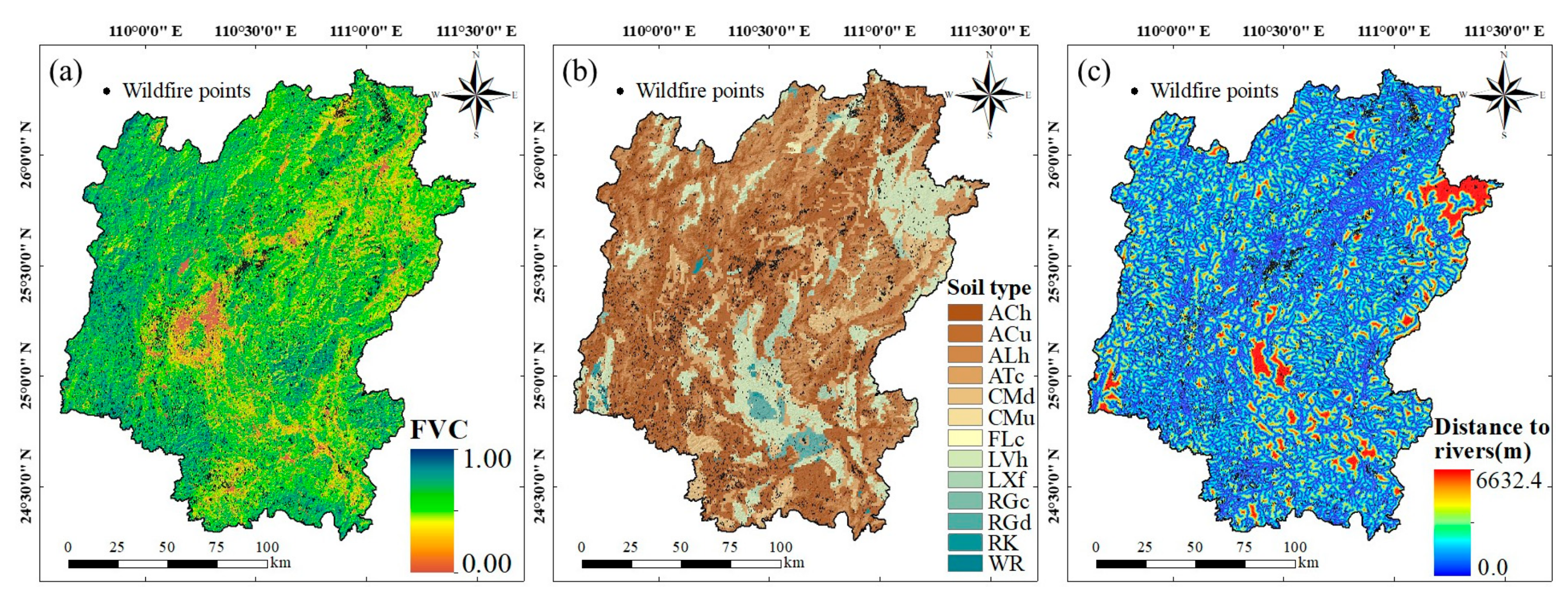
The surface environmental factors depicted in Figure 3 reflect the physical and biological environment of the land surface, which directly affect vegetation growth and water usage, thereby influencing the occurrence and spread of wildfires. Different soil types possess varying capacities for retaining moisture and conducting heat, thereby affecting the rate of vegetation growth and wildfire propagation. The distance from the water system determines human activity and vegetation growth status [44]. FVC indicates the density of surface vegetation, and a high coverage of vegetation signifies more fuel, thereby increasing the likelihood of wildfire ignition and spread [21]. The calculation formula is as follows:
F V C = N D V I N D V I m i n N D V I m a x N D V I m i n         N D V I = N I R R e d N I R + R e d
where N D V I m i n and N D V I m a x are obtained by masking the NDVI values of water bodies at a confidence level of 5% and 95%, respectively, to eliminate outliers and errors caused by soil and vegetation types, sensors, and atmospheric effects.
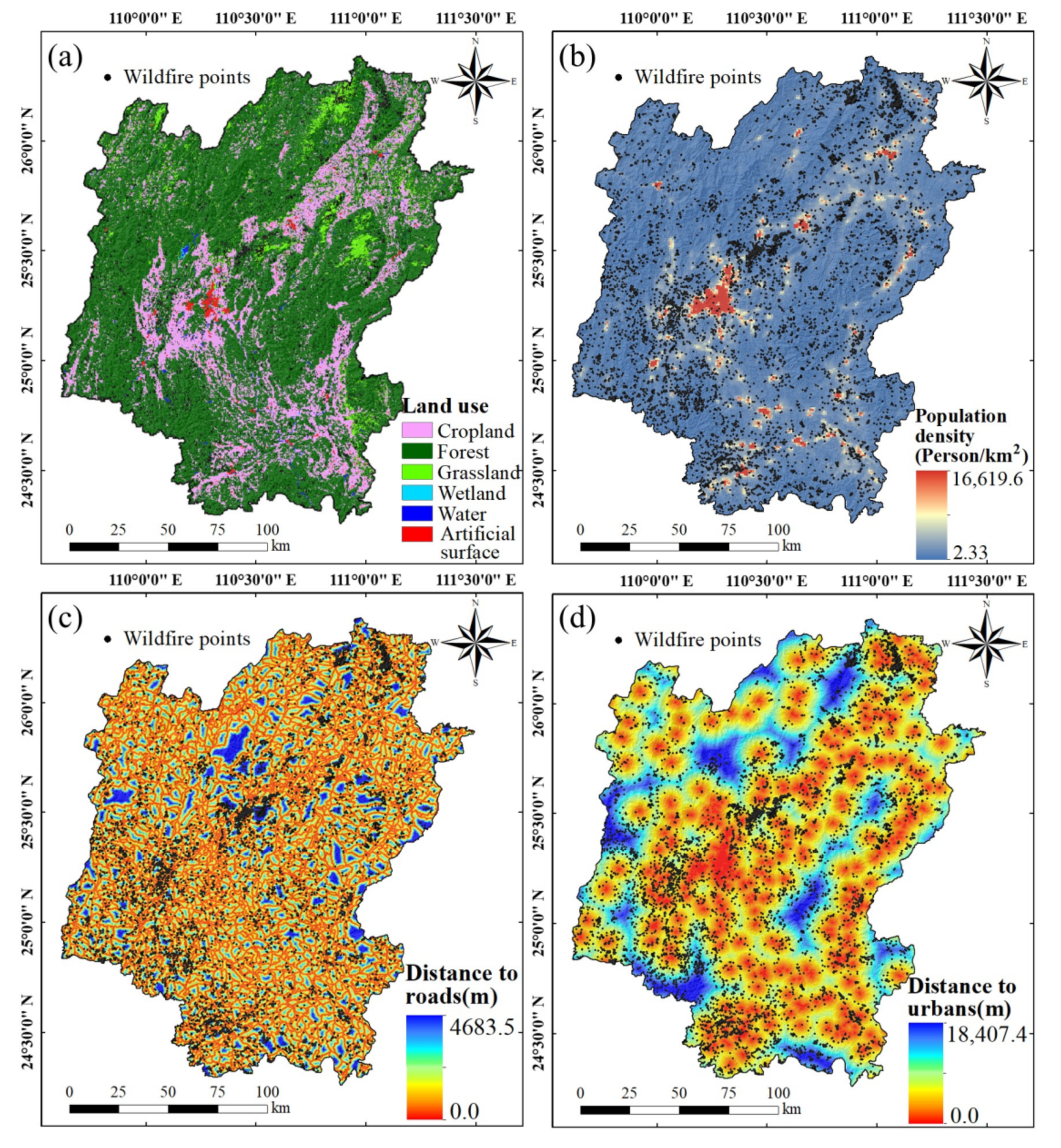
The anthropogenic factors (Figure 4) reflect the impact of human activities on wildfires [45]. Different types of land exhibit varying characteristics, such as vegetation, buildings, and human activities, which can affect the occurrence and spread of wildfires [18]. Higher population density signifies more frequent human activity, resulting in the destruction and alteration of surrounding vegetation, thus increasing the risk of wildfire occurrence [46]. The proximity of roads and residential areas to wildfire outbreaks indicates the distance between human activities and wildfires; the closer the distance, the higher the likelihood of wildfire occurrence, which also affects the speed and range of fire spread [47].
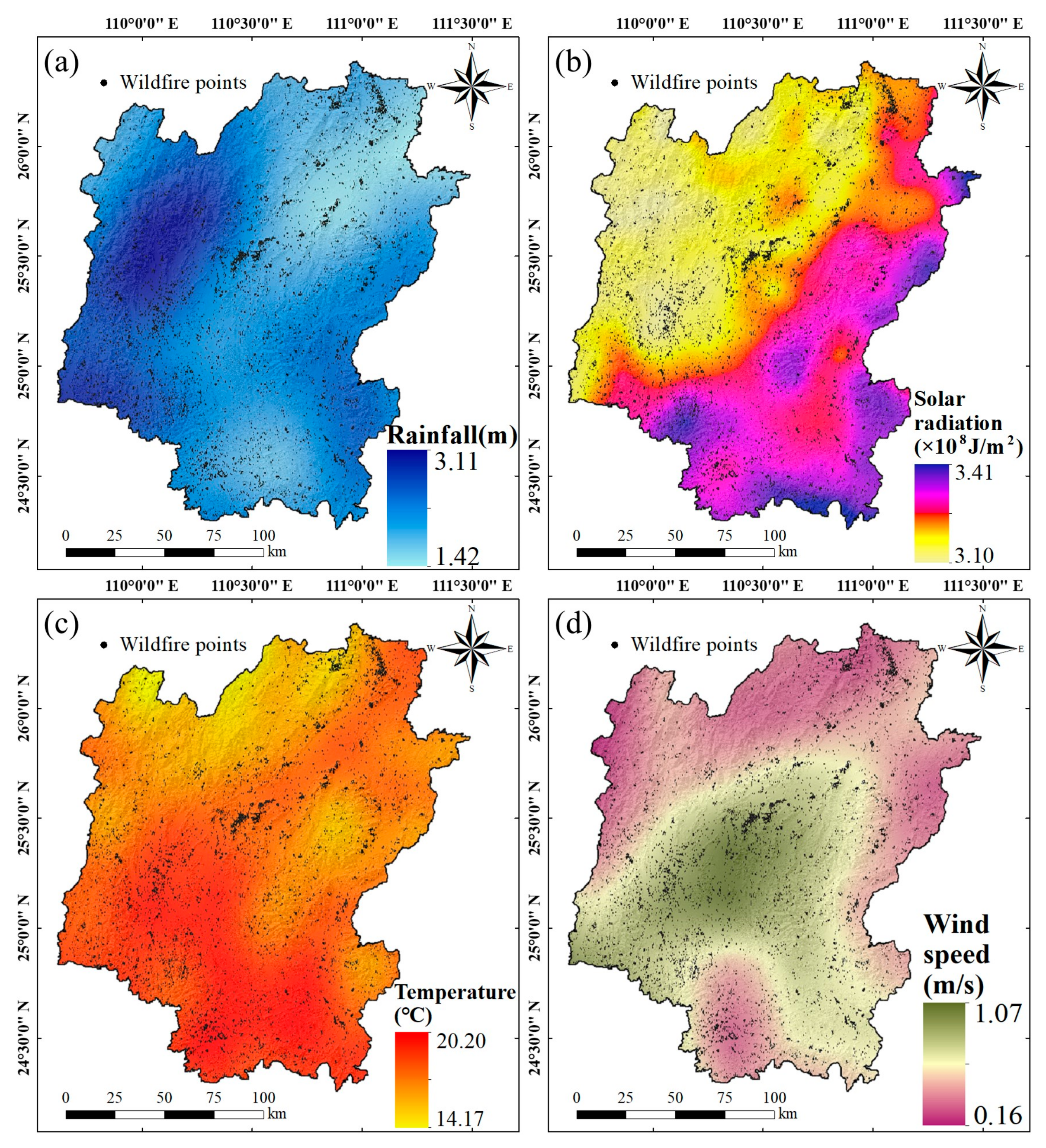
Rainfall, solar radiation, temperature, and wind speed are the primary climatic factors that influence the frequency of wildfire outbreaks and the rate of fire spread [48]. Rainfall can decrease vegetation dryness, reduce the number of ignition sources, and lower the likelihood of fire occurrence [49]. Solar radiation can dry out vegetation, increase its flammability, and consequently elevate the probability of fire outbreaks [50]. High temperature conditions can lead to vegetation withering and burning, while strong winds can accelerate the speed of fire spread [51]. The meteorological factors are shown in Figure 5.

2.4. Ecological and Urban Vulnerability Factors

2.4.1. Ecological Vulnerability Factors

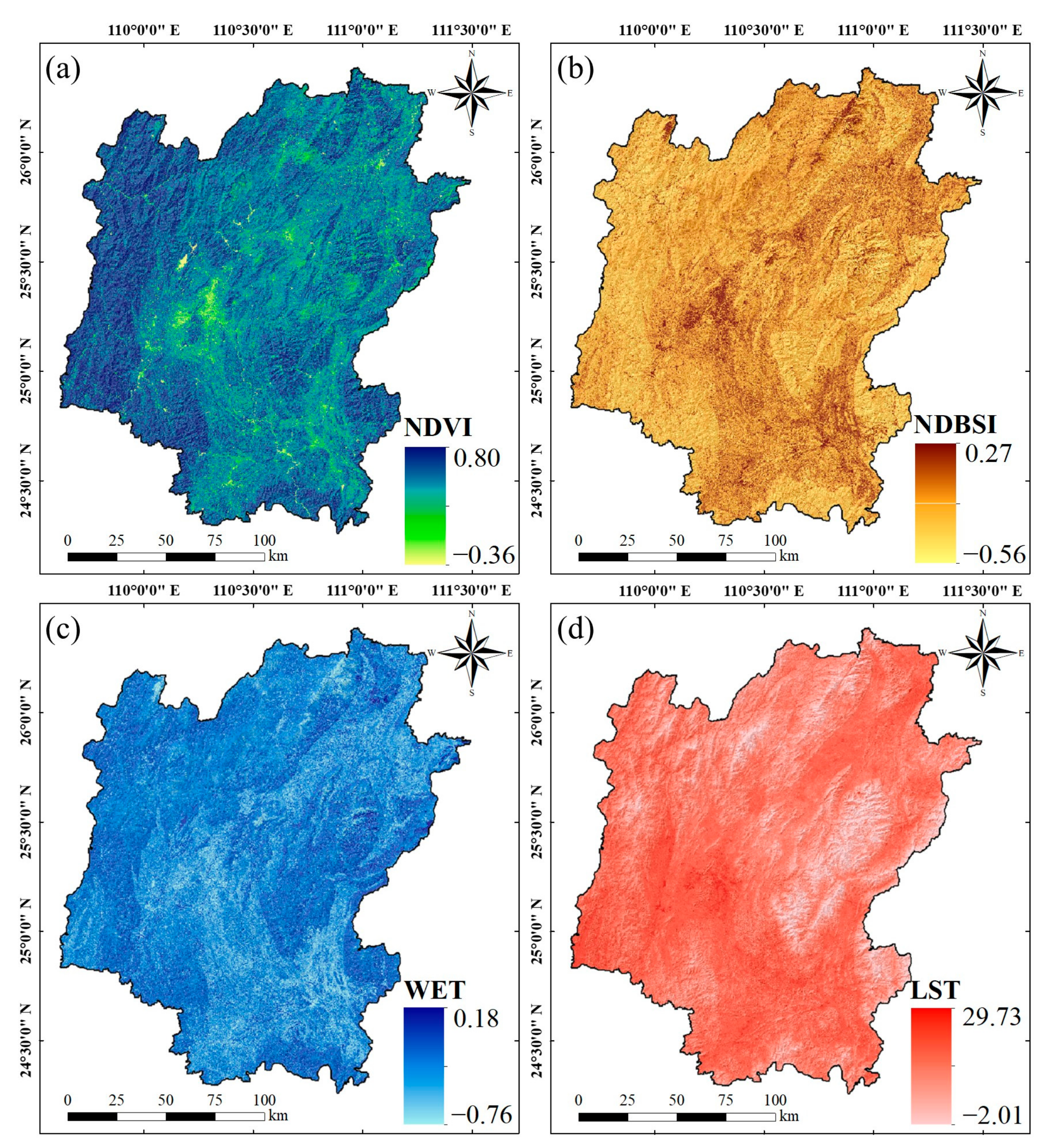
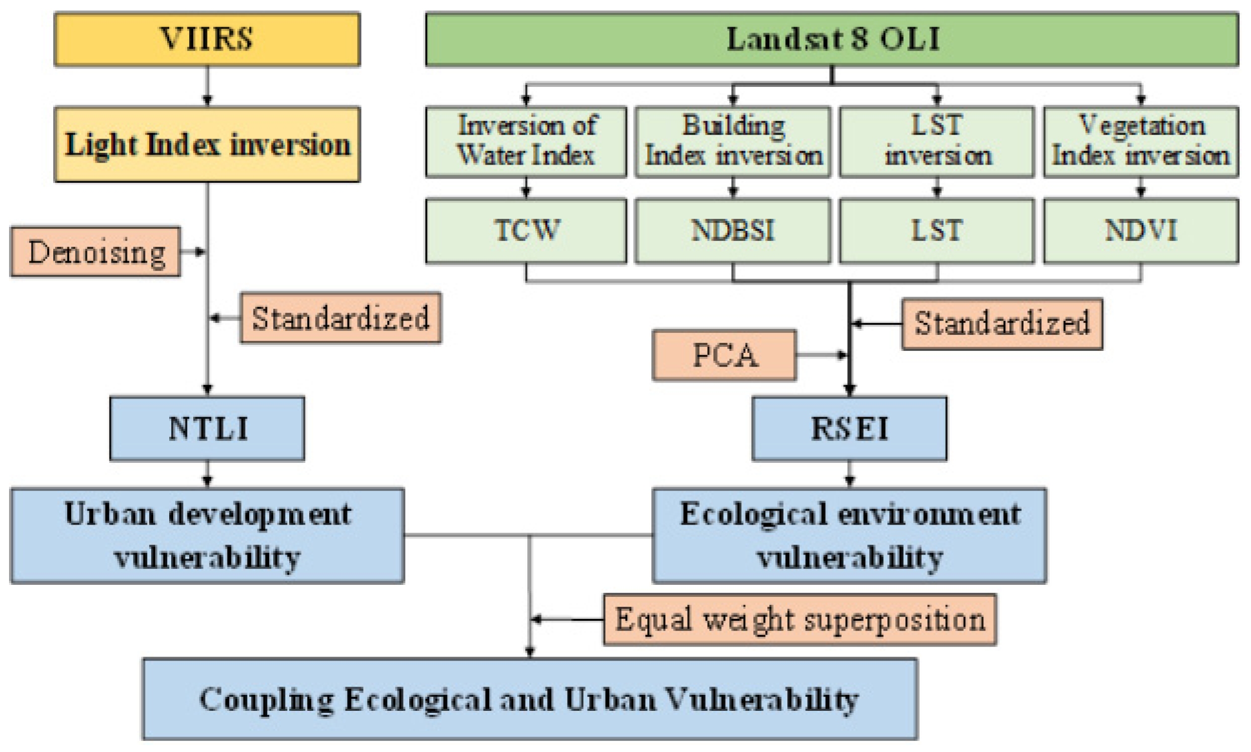
Existing studies have indicated that the Remote Sensing Ecological Index (RSEI) proposed by Xu in 2013 can objectively and rapidly evaluate the ecological environment status of a region [52,53]. RSEI integrates four indicators, namely greenness, dryness, wetness, and warmth, using principal component analysis (PCA) to assess the ecological environment quality of a specific area. Specifically, the normalized difference vegetation index (NDVI) is used to represent the greenness indicator [54]; the normalized difference built-up and soil index (NDBSI) represents the dryness indicator [55]; tasseled cap wetness (TCW) represents the wetness indicator [56]; and the land surface temperature (LST) represents the warmth indicator [57]. Based on the Google Earth Engine (GEE) platform, we used a total of 154 Landsat 8 OLI images with a cloud cover of less than 20%, covering all months from 2020 to 2022, to ensure comprehensive coverage for our analysis. We constructed RSEI by calculating the average value of all factors during this period to accurately reflect the average state of the ecological environment over the entire period (Figure 6). The formulas for calculating each indicator are presented below.
N D V I = N I R R e d N I R + R e d
I B I = 2 S W I R 1 S W I R 1 + N I R N I R N I R + R e d + G r e e n G r e e n + S W I R 1 2 S W I R 1 S W I R 1 + N I R + N I R N I R + R e d + G r e e n G r e e n + S W I R 1
S I = S W I R 1 + R e d N I R + B l u e S W I R 1 + R e d + N I R + B l u e
N D B S I = I B I + S I 2
W E T = 0.1511 × B l u e + 0.1973 × G r e e n + 0.3283 × R e d + 0.3404 × N I R 0.7117 × S W I R 1 + 0.4559 × S W I R 2
L S T = K 2 ln K 1 B T s + 1           B T s = L T L β 1 θ L β θ
where B l u e , G r e e n , R e d , N I R , S W I R 1 , and S W I R 2 represent the blue band (B2), green band (B3), red band (B4), near-infrared band (B5), shortwave infrared band 1 (B6), and shortwave infrared band 2 (B7), respectively. I B I denotes the Index-Based Built-up Index, and S I represents the Soil Index. K 1 and K 2 are calibration coefficients. L T represents the land surface temperature in the thermal infrared band of the satellite. L and L represent the upwelling and downwelling atmospheric radiance, respectively. β is the transmissivity of the thermal infrared band, and θ is the surface emissivity.

2.4.2. Urban Vulnerability Factor

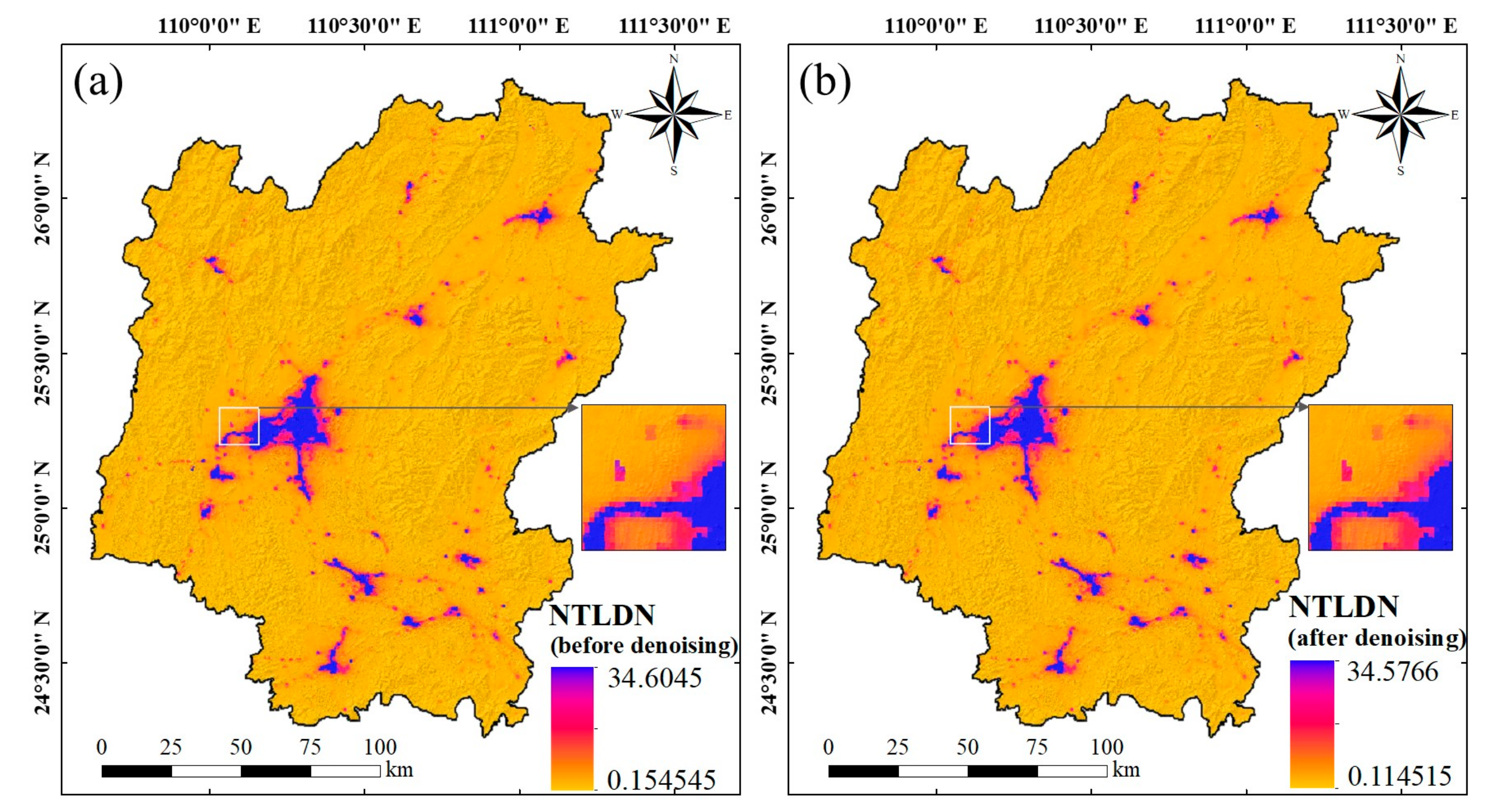
The use of nighttime remote sensing data has been widely applied to assess urban development levels, estimate population and GPD, among other fields. A higher night-time light DN (NTLDN) indicates a higher level of urban development in the area [58]. The acquisition and processing of nighttime light data was performed on the GEE platform by using the “NOAA/VIIRS/DNB/MONTHLY_V1/VCMSLCFG” function to select the “avg_rad” band to obtain the 2022 NTLDN with a resolution of 463.83 m. Despite the product being subjected to stray light correction, there still exists noise interference from unstable light sources and stray light [59]. Therefore, this study employed the S-G filtering function to remove noise from the image. The image was smoothed by setting the sliding smoothing window size and N-th derivative. Multiple experiments have shown that setting the sliding window size to 90 days and the 2nd derivative yields the best results. The results show that the radiation brightness of a certain area is strong (Figure 7a), while the denoised NTLDN becomes smoother, and noise and interference have been effectively eliminated (Figure 7b), facilitating subsequent analysis.

3. Methods

The methodology employed in this research consists of three stages.
In the first stage, wildfire susceptibility assessment was conducted following the process illustrated in Figure 8. The main steps were as follows: (1) Construction of the dataset. Acquisition and screening of historical wildfire samples; selection of negative samples for modeling; acquisition and analysis of susceptibility factors for wildfires. (2) Construction and analysis of wildfire susceptibility models. The sample dataset was randomly divided into a training set (70%) and a test set (30%). Based on the training set, wildfire susceptibility models were constructed using LR, ANN, KNN, SVR, RF, GBDT, LGBM, and XGBoost algorithms. Corresponding maps of wildfire susceptibility were generated, and the optimal model was selected based on the rationality of susceptibility zoning and predictive performance. (3) Using the SHAP interpretable method, the global feature importance, feature dependency, and local properties of typical samples of the optimal prediction model were analyzed to explore the decision mechanism of the model and summarize the laws of factors influencing wildfire occurrence.
In the second stage, the ecological and urban wildfire vulnerability assessment was conducted, and the assessment process is shown in Figure 9. First, the nighttime light data and remote sensing image data were pre-processed, and then each index was inverted to obtain the ecological environment quality and urban development level of the area. Finally, the ecological environment and urban development were coupled to construct an ecology–city wildfire disaster vulnerability model and evaluate the potential damage caused by wildfire disasters from multiple perspectives.
In the third stage, wildfire hazard risk assessment was conducted. Based on UNDHA’s disaster risk assessment method, the optimal wildfire susceptibility model was integrated with the ecological environment, urban development, and ecological–urban coupled disaster vulnerability models, respectively, and three wildfire risk models with corresponding dimensions were constructed. Moreover, the overall pattern of wildfire riskiness and the spatial distribution characteristics of risk areas in each dimension were summarized.

3.1. Multicollinearity Test

When conducting research on wildfire susceptibility, it is common to use the collected susceptibility conditioning factors as input features to train the model. However, these factors may have problems of multicollinearity, where highly correlated variables exist, affecting the stability and predictive ability of the model [60]. Therefore, when using machine learning models for wildfire susceptibility research, it is necessary to diagnose multicollinearity for these factors [61]. In this article, tolerance (TOL) and a variance inflation factor (VIF) were used for multicollinearity diagnosis. TOL reflects the correlation of a factor with other factors, while VIF is the reciprocal of TOL. When the TOL value is smaller or the VIF value is larger, it indicates a stronger correlation between the factor and other factors, and a more serious multicollinearity problem [62]. When the TOL is less than 0.1 or the VIF is greater than 10, it is considered that the factor has a multicollinearity problem and corresponding measures need to be taken to ensure the stability and predictive ability of the model [63,64].

3.2. Wildfire Susceptibility Modeling Based on Machine Learning

Due to varying availability of samples and feature data in different regions, the optimal machine learning (ML) approaches for a specific region may differ from those in other regions. Relying solely on results and recommendations from studies conducted in other regions when constructing wildfire susceptibility models for a new study in a different region can often be unreliable. Hence, this study employed eight ML algorithms to model wildfire susceptibility in Guilin, and explored the most suitable predictive model for the local context. Among these, four traditional ML algorithms, namely LR, ANN, KNN, and SVM, were utilized, along with four ensemble ML algorithms based on decision trees, namely RF, GBDT, LGBM, and XGBoost.
This research utilized historical wildfire points as positive samples, excluding areas with a high wildfire distribution density in order to obtain a selection region for negative samples. The “Create Random Points” tool in ArcGIS 10.2 was employed to randomly select 8791 negative sample data points, equivalent to the number of historical wildfire samples. Positive samples were assigned a value of “1” to indicate wildfire occurrence, while negative samples were assigned a value of “0” to denote the non-occurrence of wildfires. The positive and negative sample data were integrated to form the dataset, which was randomly divided into training and testing sets in a 7:3 ratio. The training set samples were used to build the model, with the factor attribute values of the samples as inputs and the sample attributes as outputs. Additionally, 2629 positive samples and 2646 negative samples that were not used in model construction were selected to validate the predictive performance and generalization ability of the model.

3.2.1. Logistic Regression (LR)

The LR algorithm is a machine learning technique used for classification tasks. It is based on a linear regression model that maps the linear regression outputs through a sigmoid function to estimate the probabilities of positive and negative classes in binary classification problems, constrained within the range of [0, 1] [65]. The computation formula is as follows:
P = e Y 1 + e Y
Y = B 0 + B 1 × X 1 + B 2 × X 2 + + B n × X n
where P represents the probability of wildfire occurrence, ranging from [0, 1]. X 1 , X 2 , …, X n denote the independent explanatory variables that affect wildfire events. B 0 is the intercept, and B 1 , B 2 , …, B n are the logistic regression coefficients, representing the weights of various evaluation factors.

3.2.2. Artificial Neural Network (ANN)

ANN is a sophisticated nonlinear model that is formed by interconnected neurons and possesses adaptive learning capabilities [66]. The fundamental building block of the ANN is the neuron, which receives multiple input signals and produces an output by summing the weighted inputs using an activation function. The primary algorithm employed in ANN is the backpropagation algorithm, which continuously adjusts the weights and biases parameters by computing the gradient of the error, gradually aligning the model’s predicted results with the actual results [67]. The mathematical expression is
y i = σ j = 1 n w i j x j + b i
where y i represents the output of neuron i , σ denotes the activation function, w i j represents the connection weight between input x j and neuron i , and b i represents the bias of neuron i . The input values for the input layer are denoted as x j , while the output values for the output layer are denoted as y i . The output values of the hidden layer serve as the input values for the next layer.

3.2.3. K-Nearest Neighbor (KNN)

KNN, introduced by Cover and Hart in 1967, is a supervised learning algorithm [68]. Its fundamental idea is to determine the K closest training samples to a given unclassified sample by calculating the distances between the samples. Then, utilizing the labels of these K training samples, a voting or weighted voting approach is employed to determine the class or value of the unclassified sample [69]. For a test sample x, assuming its nearest K neighbors are x1, x2, …, xk and corresponding outputs are y1, y2, …, yk, the predicted outcome of the KNN regression is
y ^ = 1 K i = 1 K y i
where y ^ represents the predicted value, and K denotes the number of neighbors.

3.2.4. Support Vector Regression (SVR)

SVR is a regression algorithm based on support vector machines, with the objective of seeking a hyperplane that maps the feature space to a higher-dimensional space, minimizing the error between corresponding function values and the true values [70]. It controls the allowable degree of error by setting boundaries, known as support vectors, which differentiate it from traditional linear regression. Unlike linear regression, SVR employs kernel functions to handle nonlinear problems, enabling the adaptive determination of nonlinear relationships in high-dimensional space. The formula for minimizing the error is
min w , b , ϵ i , ϵ i 1 2 w 2 + C i m ϵ i + ϵ i
y i w T ϕ x i b ϵ i
w T ϕ x i + b y i ϵ i
ϵ i , ϵ i 0
where w is the normal vector of the hyperplane, ϕ x is the function that maps sample points x to a high-dimensional space, b is the bias term, C is the regularization coefficient, ϵ i and ϵ i are the slack variables, y i is the true value of the sample points, and m is the number of sample points.

3.2.5. Random Forest (RF)

RF is an ensemble learning algorithm based on decision trees, whose decision trees, serving as supervised classifiers, can provide decisions at multiple levels. Due to the reduced instability observed in constructing a single decision tree, the ensemble integrates the results of classification and regression trees, thereby mitigating the discontinuity of a single tree and maintaining constant prediction probabilities [71]. Compared to the aforementioned four models, RF exhibits lower sensitivity to multicollinearity among factors. It possesses exceptional robustness, effectively avoiding overfitting problems, and helps reduce the impact of outliers on modeling results.

3.2.6. Gradient Boosting Decision Tree (GBDT)

The GBDT algorithm is another ensemble algorithm, which iteratively trains decision tree models and progressively improves their performance through residual analysis [72]. Specifically, the algorithm first uses a simple model to fit the training data, and then calculates the residual of the model on the training data. Subsequently, the algorithm uses a new decision tree model to fit the residual and obtain a new model. The algorithm repeats this process, generating a new model at each iteration, and adding up the results of all previous models to form the final model [73].

3.2.7. Light Gradient Boosting Machine (LGBM)

LGBM is a machine learning algorithm based on GBDT [74]. In contrast to GBDT, LGBM employs an algorithm based on histograms and a leaf-wise growth strategy, thereby reducing memory consumption and computation time. Moreover, LGBM adopts various strategies, such as regularization, to prevent overfitting, and supports multi-threading and parallel computing, facilitating the processing of massive data and high-dimensional features. This results in faster processing, lower memory consumption, and improved model accuracy.

3.2.8. eXtreme Gradient Boosting (XGBoost)

XGBoost is an optimized and extended algorithm based on the gradient boosting algorithm, which was designed and proposed by Chen in 2016 [75]. It adds a penalty term on the basis of GBDT to reduce model variance and effectively prevent overfitting. XGBoost models and predicts high-uncertainty samples by creating multiple decision trees at different time intervals. In addition, adjusting multiple hyperparameters can reduce the risk of overfitting and prediction variability, thus improving accuracy [76]. The objective function of XGBoost is as follows:
O t = j = 1 T G j w j + 1 2 H j + λ w j 2 + λ T
where O t represents the maximum reduction in the objective after specifying the tree structure at the t -th iteration, where smaller values indicate better tree structures. T denotes the number of leaf nodes, w j represents the weight of the j -th leaf node, and G j and H j , respectively, represent the sum of first-order and second-order derivatives of the j -th sample.
In this study, grid search and cross-validation were employed to adjust the hyperparameters of the models for reliable prediction results. Table 2 represents the hyperparameters of each algorithm and shows the values of these hyperparameters.

3.3. Performance Assessment of Susceptibility Models

In studies of wildfire susceptibility, susceptibility is typically treated as a binary classification problem, where samples are divided into wildfire and non-wildfire categories [77]. To select the optimal model from eight models, multiple metrics were used to comprehensively evaluate the predictive performance of each model. The receiver operating characteristic (ROC) curve and its area under the curve (AUC) are one of the most commonly used metrics for evaluating the performance of binary classification models [78]. AUC can be used to compare the performance of different models, that is, to evaluate the model’s ability to correctly predict the presence or absence of wildfires. The larger the AUC value, the better the model’s performance, and when the AUC value is greater than 0.9, it indicates that the model can distinguish wildfires and non-wildfires very well, and has very high discrimination ability [79,80]. Precision refers to the proportion of samples predicted as wildfires that are actually wildfires; sensitivity refers to the proportion of actual wildfire samples that are correctly predicted as wildfires, and specificity refers to the proportion of actual non-wildfire samples that are correctly predicted as non-wildfires. An F1-score is the harmonic mean of precision and sensitivity, reflecting the comprehensive prediction performance of the model for wildfire samples. Accuracy refers to the proportion of samples that the model correctly predicts, reflecting the overall prediction performance of the model. The formulas for calculating the above metrics are as follows:
A U C = 1 2 × T P T P + F N + T N T N + F P
P r e c i s i o n = T P T P + F P
S e n s i t i v i t y = T P T P + F N
S p e c i f i c i t y = T N T N + F P
F 1 s c o r e = 2 × P r e c i s i o n × S e n s i t i v i t y P r e c i s i o n + S e n s i t i v i t y
A c c u r a c y = T P + T N T P + F N + T N + F P
where T P represents the count of wildfires classified as wildfires; T N represents the count of non-wildfires classified as non-wildfires; F N represents the count of wildfires misclassified as non-wildfires; and F P represents the count of non-wildfires misclassified as wildfires.
Furthermore, the prediction error of the model was assessed by calculating the root mean square error (RMSE) between the predicted outcomes of wildfire samples (1), non-wildfire samples (0), and all samples (All), and the actual attributes [81,82]. The computation formula is as follows:
R M S E A l l ; 1 ; 0 = 1 N i = 1 N Y i f X i 2
where N represents the total number of samples, and Y i and f X i represent the actual value and predicted value, respectively, for the i -th sample.

3.4. SHapley Additive exPlanations (SHAP) Method

SHAP (SHapley Additive exPlanations) is a method proposed by Lundberg and Lee in 2017 to explain the predictive results of machine learning models. The core of the matter is to compute the contribution of each feature to the model’s prediction results [83,84]. It is based on the idea of the Shapley value in game theory, which is transformed into feature importance by calculating the Shapley value of each feature for the predicted outcome of the model [85]. The analysis results can help us understand the impact level (direction and strength) of each feature on the predictive results of the entire dataset, and help us identify which features have a significant impact on the model’s predictive results [86,87]. Due to its theoretical interpretability, the SHAP method has been widely used in interpreting black-box models. The Shapley value is calculated using the following formula:
ϕ j = 1 M i = 1 M S x i / j S ! x i S 1 ! x i ! f S j x i f S x i
where x i represents the i -th sample; j represents one of the features; S represents the subset of features that does not include feature S ; f S x i represents the model’s prediction output after removing feature S ; f S j x i represents the model’s prediction output after adding feature j; and M is the number of samples. The Shapley value represents the contribution of feature j to the prediction output for sample x i , which is equal to the difference between the prediction outputs considering and not considering feature j , multiplied by the weight of the sample subset when considering feature j , and then averaged. In this study, the SHAP (SHapley Additive exPlanations) method was used to analyze the direction and contribution level of each susceptibility conditioning factor to wildfire susceptibility prediction results in both global and local dimensions.

3.5. Ecological and Urban Vulnerability Modeling

According to the vulnerability definition released by the United Nations in 1992, “The degree of loss that may be caused by the potential damage phenomenon,” refers to the degree of vulnerability demonstrated by the carriers of human, material, and environmental elements within the region under the influence of disasters [88]. This paper analyzes wildfire vulnerability based on three dimensions: ecological environment quality, urban development level, and the coupling of ecology and urbanization. Based on research, the Remote Sensing Ecological Index (RSEI) can represent the ecological environment condition, while the Night-Time Lights Index (NTLI) can better represent the level of urban development [34,89]. NTLI is obtained through normalization processing by NTLDN, and the RSEI calculation formula is as follows:
N i = I I m i n I m a x I m i n
R S E I 0 = P C A f L S T , W E T , N D B S I , N D V I
R S E I = R S E I 0 R S E I 0 m i n R S E I 0 m a x R S E I 0 m i n
where N i represents the normalized values of four indicators, including heat, dryness, humidity, and greenness; I represents the pixel values of the corresponding indicators; I m i n represents the minimum pixel value of the indicator; I m a x represents the maximum pixel value of the indicator; R S E I 0 represents the initial remote sensing ecological index based on principal component analysis (PCA); R S E I 0 m i n represents the minimum pixel value of the first principal component; R S E I 0 m a x represents the maximum pixel value of the first principal component; and R S E I represents the standardized remote sensing ecological index, ranging from 0 to 1.
In this study, it was acknowledged that both the ecological environment and urban development are equally significant in assessing the wildfire disaster vulnerability in Guilin. Therefore, weights of 0.5 were assigned to both the ecological environment condition and urban development level to couple the two factors. The calculation formula was as follows:
V R N _ i = 0.5 × V R _ i + 0.5 × V N _ i
where V R N _ i represents the wildfire vulnerability result of the i -th unit, which integrates ecological environment and urban development, while V R _ i and V N _ i , respectively, denote the ecological environment vulnerability result and urban development vulnerability result of the i -th evaluation unit.

3.6. Wildfire Risk Modeling

The conventional definition of risk originates from the fields of natural science, engineering, and economics. It defines risk as the probability of negative consequences resulting from disasters [90]. Additionally, the “Risk = Hazard/Susceptibility × Vulnerability” formula proposed by the United Nations Department of Humanitarian Affairs (UNDHA) in 1991 marked the entry of disaster risk assessment into a quantitative stage [91]. Currently, this method is widely applied in the assessment of natural disaster risks such as landslides and floods, achieving a certain effectiveness [92,93].
Wildfire susceptibility was coupled with the results of ecology, city, and ecology–city vulnerability assessments. By calculating the risk levels of wildfire disaster damage to the ecological environment, urban development, and the ecology–city category, respectively, the risk of wildfire disaster in Guilin was evaluated and analyzed in three dimensions.
R i = S i × V i
where R i represents the risk index of the i -th assessment unit, while S i and V i , respectively, denote the susceptibility and vulnerability (ecological/urban/ecology–city) indices of the i -th assessment unit.

4. Results

4.1. Wildfire Susceptibility Assessment

4.1.1. Multicollinearity Test Results

Table 3 shows the results of multicollinearity analysis among the conditioning factors of wildfire susceptibility. The TOL values for all 17 factors were above 0.1, and the VIF values were below 10.0. The lowest TOL score for elevation was 0.304, and the highest VIF score was 0.287. These findings indicated that there is no multicollinearity among the susceptibility factors, mitigating the risk of model accuracy degradation due to inadequate data quality. Hence, all 17 factors could be employed in the modeling and evaluation of wildfire susceptibility.

4.1.2. Wildfire Susceptibility Map

This study utilized eight machine learning methods combined with 17 susceptibility factors to construct a prediction model for wildfire susceptibility in Guilin, and predicted the susceptibility values for the entire region. Furthermore, the predicted values for all units within the study area were visualized using ArcGIS 10.2 software to generate corresponding maps of wildfire susceptibility. In order to facilitate the direct comparison of wildfire susceptibility maps generated by different algorithms, it is necessary to ensure that specific levels of susceptibility have the same range of wildfire occurrence probabilities in each model’s susceptibility map. Therefore, we adopted a uniform classification scheme based on the intervals of [~, 0.20], (0.20, 0.40], (0.40, 0.60], (0.60, 0.80], and (0.80, ~] to divide the wildfire susceptibility in the study area into five levels: very low, low, moderate, high, and very high. The wildfire susceptibility models based on traditional machine learning methods are shown in Figure 10, while those based on ensemble machine learning are shown in Figure 11. Visually, the zoning patterns of wildfire susceptibility based on different models had certain similarities, but there were significant differences in detail. The high-susceptibility areas of all eight machine learning models were distributed in the central, northeast, south, and southwest parts of the area, while the susceptibility in the north, central south, central east, and southeast regions was relatively low. In addition, compared with LR, ANN, KNN, and SVR, most sample points in the remaining four ensemble machine learning models were located in fewer areas of high susceptibility, and exhibited a superior fitting performance when predicting wildfires.
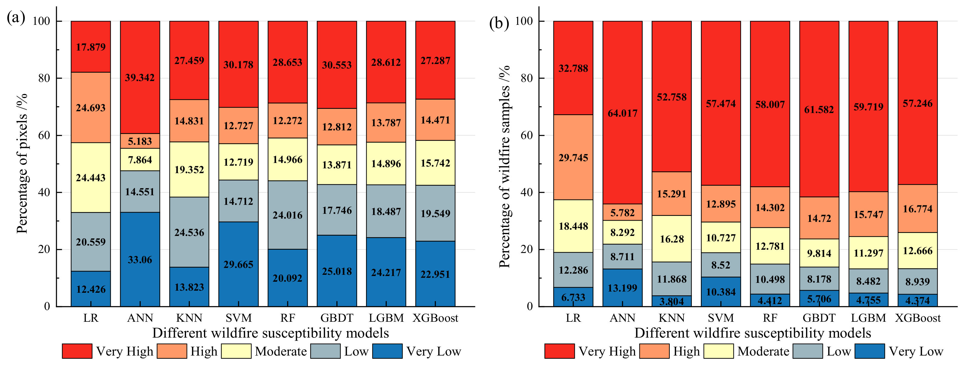
To assess the disparities in the susceptibility delineation details among the models, this study meticulously compiled data on the proportion of area and sample quantity for each susceptibility level in different models (Figure 12). Across all models, the ranking of the proportion of high- and very-high-susceptibility areas was as follows, in ascending order: RF (40.925%) < XGBoost (41.758%) < KNN (42.290%) < LGBM (42.399%) < LR (42.572%) < SVM (42.904%) < GBDT (43.365%) < ANN (44.525%). In addition, the ranking of the wildfire samples included, in descending order, was as follows: GBDT (76.303%) > LGBM (75.466%) > XGBoost (74.021%) > RF (72.309%) > SVM (70.369%) > ANN (69.798%) > KNN (68.049%) > LR (62.533%). It is evident that, in comparison to the other models, the very-high-susceptibility areas of the four ensemble ML models are smaller but contain more wildfire samples. Among them, the XGBoost model exhibits a higher level of reliability in zoning results by covering a larger number of wildfire samples whilst possessing fewer areas of high susceptibility.
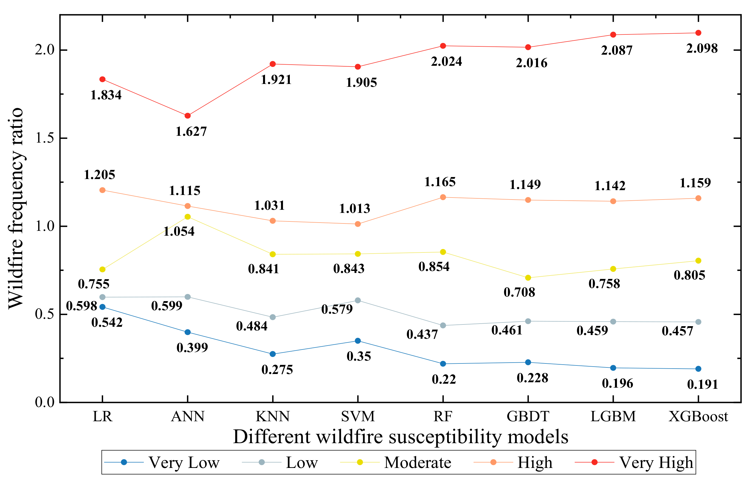
The wildfire frequency ratio was introduced to improve the fit of the wildfire samples to the susceptibility zoning results evaluated by each model. It was calculated by the percentage of wildfire samples falling into each level of susceptibility zone, combined with the proportion of the area of each level of susceptibility zone. A higher ratio indicates that more wildfire samples are located in smaller susceptibility zones, resulting in more reasonable zoning results [94]. As shown in Figure 13, the frequency ratios of all models increase with the increase in susceptibility levels, and the zoning results are reasonable. Moreover, the frequency ratios of RF, GBDT, LGBM, and XGBoost models in the high-susceptibility zones are all greater than 2.0, indicating a good zoning effect for wildfires. Among them, compared with other models, the XGBoost model has the lowest frequency ratio (0.191) in the very-low-susceptibility zones and the highest frequency ratio (2.098) in the very-high-susceptibility zones, resulting in a better fit of the wildfire susceptibility zoning results to the wildfire samples and the most reasonable zoning results.

4.1.3. Model Performance Assessment

The proportion of sample data in different susceptible areas can only reflect the predictive accuracy of the model under specific threshold conditions. Considering that the ROC curve is not affected by the threshold and can clearly indicate the relationship between the cumulative percentage of wildfire occurrence and the wildfire susceptibility index, we evaluated the overall performance and generalization ability of different models using the ROC curve (Figure 14). The AUC values of the ROC curves for the RF, GBDT, LGBM, and XGBoost models were all greater than 0.90, indicating that the ensemble machine learning (ML) model exhibited superior predictive performance compared to traditional ML models. Among them, the XGBoost model demonstrated the highest AUC value of 0.927, surpassing all other models in terms of overall predictive performance.
After validating the overall performance of the models, multiple metrics were utilized to evaluate the predictive accuracy of various wildfire susceptibility models on wildfire samples, as presented in Table 4. Among the eight models examined, LR, ANN, KNN, and SVR models exhibited relatively lower predictive accuracy for both positive and negative samples, with overall predictive accuracies of 0.735, 0.814, 0.807, and 0.821, respectively. On the other hand, the GBDT model demonstrated high predictive accuracy for both positive and negative samples, with an overall predictive accuracy of 0.853. The RF model performed well in terms of predictive accuracy for negative samples, but relatively poorer in terms of predictive accuracy for wildfire samples, with overall predictive accuracies of 0.853. Meanwhile, the LGBM and XGBoost models showed the best predictive accuracy for wildfire samples, although LGBM’s predictive accuracy for negative samples was lower than that of XGBoost, with overall predictive accuracies of 0.852. Notably, the XGBoost model, while ensuring the highest predictive accuracy for wildfire samples, also demonstrated good predictive accuracy for negative samples, with an overall classification accuracy of 0.890 and an F1-score of 0.852, indicating superior discriminative ability for wildfire samples and increased reliability. Additionally, the XGBoost model exhibited lower RMSE (All), RMSE (1), and RMSE (0) values compared to other models, indicating smaller predictive errors for wildfire samples, negative samples, and all samples, thereby aligning more closely with the real situation. In conclusion, the XGBoost model displayed the best predictive performance, followed by the LGBM, GBDT, and RF models, while the predictive performance of the four traditional models (LR, ANN, KNN, and SVR) was relatively poor.

4.1.4. Results of SHAP Method

Consequently, considering the analysis of the rationality of susceptibility zoning results and the predictive performance of the eight models mentioned previously, the wildfire susceptibility evaluation results obtained from the XGBoost model were superior to other models, positioning the XGBoost model as the optimal model in this study. Therefore, we employed the data-driven SHAP interpretability method to explain and analyze the decision mechanism of the XGBoost model for wildfire susceptibility.
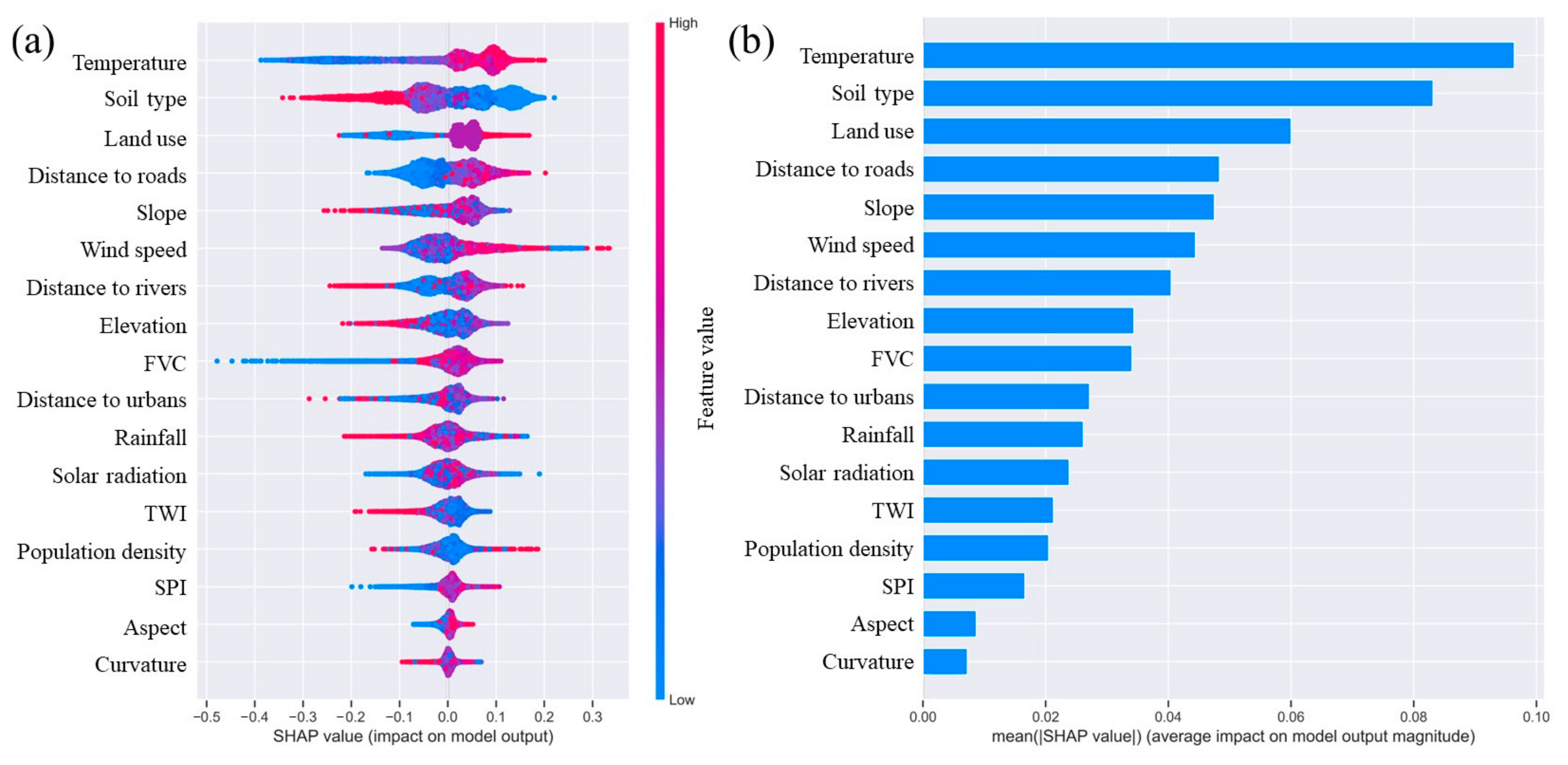
Figure 15 illustrates the directional effects and importance levels of each factor on the prediction results of wildfire susceptibility. Figure 15a plots the Shapley values of each factor for each sample. The horizontal axis displays the Shapley values, where larger values indicate a greater impact on the prediction results. Positive values represent a positive influence, while negative values represent a negative influence. Red represents high attribute values, while blue represents low attribute values. For instance, when NDVI values are high, Shapley values are generally large, indicating that an increase in temperature is conducive to the occurrence of wildfires. When rainfall is high, Shapley values are small, indicating that an increase in rainfall in the region would reduce the likelihood of wildfires. Continuous factors such as temperature, distance to roads, wind speed, FVC, and SPI have varying degrees of positive influence on the prediction of wildfire susceptibility. Elevation, rainfall, TWI, and curvature have varying degrees of negative influence. Slope, distance to rivers, distance to urban areas, solar radiation, and population density have more complex interval monotonicity or no clear positive or negative effects on wildfire susceptibility prediction results. For discrete factors, the likelihood of wildfires occurring is higher on slopes facing southwest, south, and southeast. Acidic soils (such as Ach and Acf) have a strong promoting influence on wildfire occurrence compared to other soil types. Forest and grassland are more prone to wildfire disasters than other land types.
The factor importance ranking results were obtained by calculating the average Shapley absolute values of all samples for each factor in Figure 15a, as shown in Figure 14b. The results indicate that temperature, soil type, land use, distance to roads, slope, wind speed, distance to rivers, elevation, and FVC are the most important factors affecting wildfire susceptibility prediction in Guilin, while the impact of the other eight factors is relatively small.
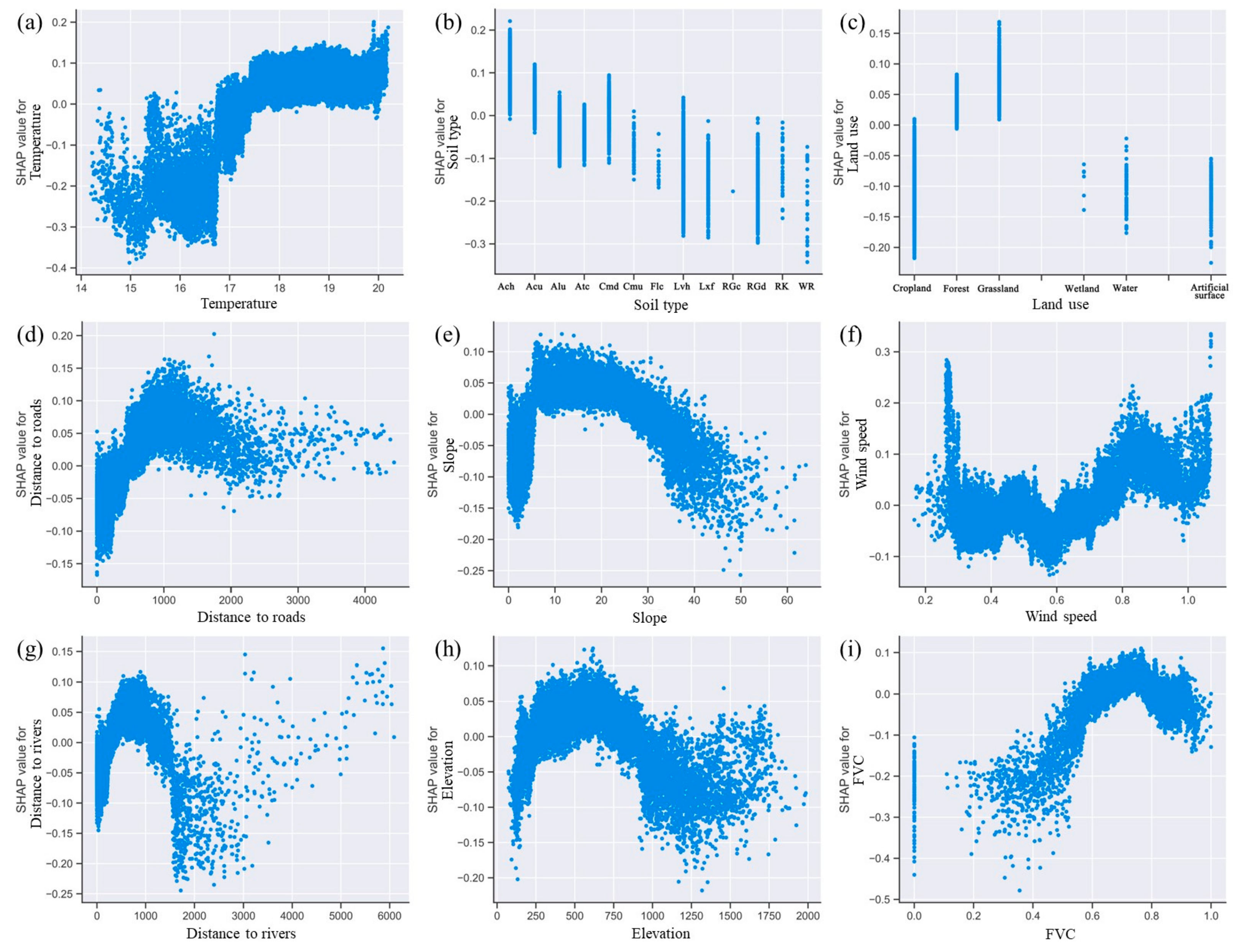
Factor dependence analysis can effectively describe the marginal effects of factors on the predictive results of the model. Single dependency analysis illustrates the impact of a single factor on the prediction of wildfire susceptibility [95,96]. Figure 16 presents the individual dependence of the nine most significant factors in the model. The horizontal axis represents the attribute values of the factors, while the vertical axis represents the Shapley value of the sample associated with the attribute value. Through analysis, it is observed that
(1)
Temperature positively influences the occurrence of wildfires, as higher temperatures result in larger Shapley values and a greater likelihood of wildfire outbreaks. When the temperature exceeds 17.3 °C, the Shapley value is generally greater than 0, indicating higher susceptibility to wildfire disasters.
(2)
Except for FLc, LXf, RGc, RGd, RK, and WR soil types, all other soil types have the potential to experience wildfires. Among them, soil types such as Ach and Acf generally have a Shapley value greater than 0, making them more susceptible to wildfire disasters.
(3)
Compared to cropland and forest, samples belonging to grassland have the highest Shapley value, making them more susceptible to wildfire disasters.
(4)
Overall, the Shapley value of samples increases with an increase in the distance to roads. When the distance to roads is greater than 500 m, the Shapley value is greater than 0, indicating that wildfire disasters in Guilin are more likely to occur in areas far from human activity.
(5)
When slope is within the range of [5°, 25°], the Shapley value is greater than 0, indicating a positive effect on the occurrence of wildfires. The mountains within this range of inclination tend to receive more direct sunlight and are more exposed to natural winds, thus causing vegetation to dry out faster and become more combustible.
(6)
When wind speed is in the interval of [0 m/s, 0.6 m/s], the Shapley value decreases with the increase in the wind speed, while when the wind speed is greater than 0.6 m/s, the wind speed has a positive impact on the occurrence of wildfires, and the Shapley value of the sample increases with the increase in the wind speed. Moreover, when the wind speed is greater than 0.8 m/s, the Shapley value is generally greater than 0, indicating a higher probability of wildfire disasters.
(7)
When the distance to rivers is in the range of (0, 1000 m), the Shapley value of the sample gradually increases and is greater than 0; however, when the distance to rivers is greater than 1000 m, the Shapley value of the sample shows a downward trend, indicating that the area near the river is more prone to wildfire disasters.
(8)
There is a non-monotonic relationship between elevation and wildfire. The samples with Shapley value greater than 0 are basically located in the range of (250 m, 1000 m), and the probability of wildfires is high; when the elevation is greater than 1000 m, the possibility of wildfires is reduced.
(9)
FVC exerts a positive influence on wildfire occurrence overall. When FVC is in the range of (0.6, 0.8), the Shapley value is greater than 0, and the probability of a wildfire disaster is greater.
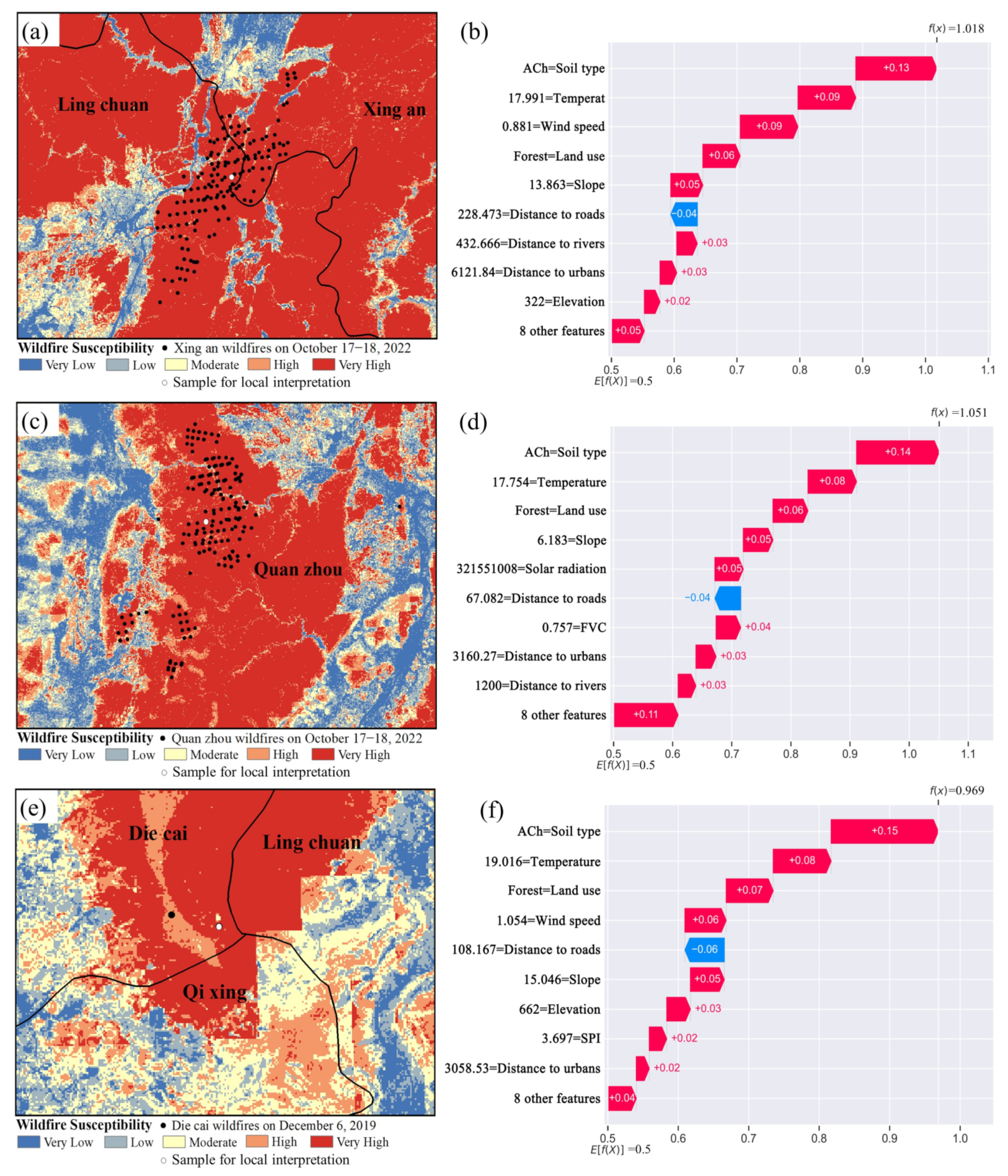
The SHAP method not only provides a global interpretation of the impact of various factors on the overall susceptibility of wildfires, but also enables a local analysis of how the model predicts the impact of different factors on individual samples [97]. We collected information on major wildfire disasters in Guilin from 2013 to 2022 through mainstream media. It was combined with wildfire susceptibility prediction models and sample data to perform local interpretation analysis. Table 5 presents detailed information on three specific historical major wildfires that were selected as representative samples. The latitude and longitude coordinates provided in the table indicate the location of each individual sample within the burned areas. Figure 17a–c represents the local wildfire susceptibility maps for the three wildfire incidents, while Figure 17d–f depicts the local interpretation plots for the corresponding samples in each case. The names and attribute values of the main influencing factors of the samples are displayed on the left-hand side of the figure. The central red color represents the strength of the positive factors that promote wildfire occurrence, while the blue color represents the opposing factors. The positive and negative strengths of the various factors offset each other, leading to the final predicted value displayed in the upper part of the figure. Through analysis, it can be inferred that
(1)
For wildfire case 1, soil type, temperature, wind speed, and land use have a significant positive effect, while slope, distance to rivers, distance to urban areas, and elevation have a minor positive effect. Distance to roads has a significant negative effect, and the remaining eight factors contribute a positive effect of 0.05. The final predicted wildfire susceptibility value is 1.018, and it is classified as a wildfire.
(2)
For wildfire case 2, soil type, temperature, land use, and slope have a significant positive effect, while solar radiation, FVC, distance to urban areas, and distance to rivers have a minor positive effect. Distance to roads has a significant negative effect, and the remaining eight factors contribute a positive effect of 0.11. The final predicted wildfire susceptibility value is 1.051, and it is classified as a wildfire.
(3)
For wildfire case 3, soil type, temperature, wind speed, and land use have a significant positive effect, while slope, elevation, SPI, and distance to urban areas have a minor positive effect. Distance to roads has a significant negative effect, and the remaining eight factors contribute a positive effect of 0.04. The final predicted wildfire susceptibility value is 0.969, and it is classified as a wildfire.
The local interpretation results of typical wildfire samples are consistent with the results of factor dependence analysis. This not only improves the credibility of the wildfire susceptibility analysis results but also effectively verifies the prediction stability of the model for typical wildfire disasters, providing a theoretical basis and targeted recommendations for the prevention and control of wildfire disasters in Guilin.

4.2. Wildfire Vulnerability Assessment Considering Ecology and City

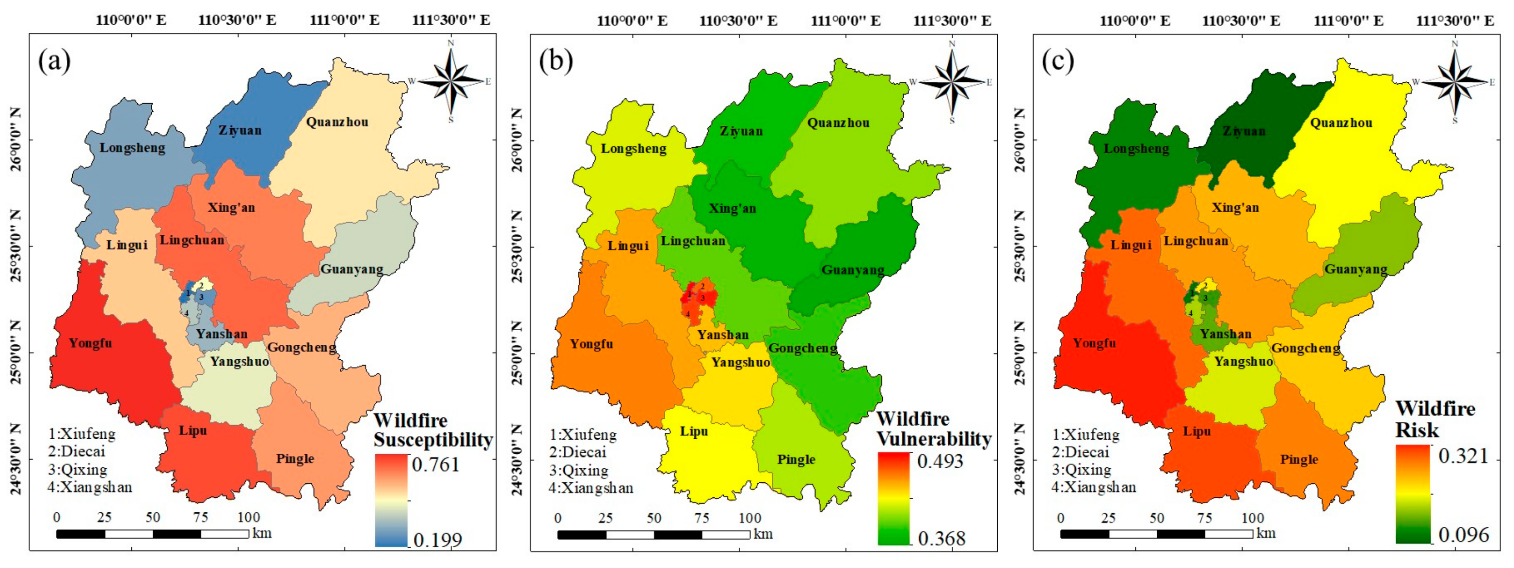
This paper conducted an analysis of wildfire vulnerability from three perspectives: ecological environment, urban development, and ecology–city coupling. The corresponding wildfire vulnerability maps are shown in Figure 18.
Regarding the ecological environment, the RSEI was constructed using PCA based on four indicators, namely NDVI, TCW, LST, and NDBSI, to analyze the recent status of the ecological environment of Guilin. The contribution rate of the first principal component was 95.74%, indicating that it contains most of the information of the four indicators. Therefore, the first principal component was utilized to construct the RSEI. In terms of ecological quality evaluation, the average value of RSEI in Guilin is 0.780 (∈[0.6, 0.8]), indicating a good quality of ecological environment in Guilin [98]. In terms of disaster vulnerability, the southern, western, and northeastern parts of Guilin exhibit relatively higher vulnerability of the ecological environment compared to other areas. The spread of wildfires in these areas can cause significant damage to the ecological environment.
Regarding urban development, the distribution of NTLI in the study area was utilized to delineate the extent of social and economic activities as well as urban expansion. The higher the value, the higher the population and level of economic activities [99]. The results show that Xiufeng, Diecai, Xiangshan, and Qixing Districts, as well as their surrounding counties, and the central areas of each county, have denser population and road distributions and a higher level of economic development compared to other areas. Therefore, when disasters occur, the above-mentioned areas are more vulnerable to population and economic losses.
For the coupled model of ecological environment and urban development, the mean vulnerability result is 0.395, indicating a moderate to low degree of vulnerability to ecology–city disasters in this area. From the vulnerability results of Figure 17, it can be seen that the vulnerability model based on ecology–city coupling covers high-vulnerability areas more comprehensively, and the division between low vulnerability and high vulnerability is more distinct, with more detailed information, thus providing a more comprehensive and accurate description of the loss situation of the ecological environment and population and economic activities when disasters occur.

4.3. Wildfire Risk Assessment

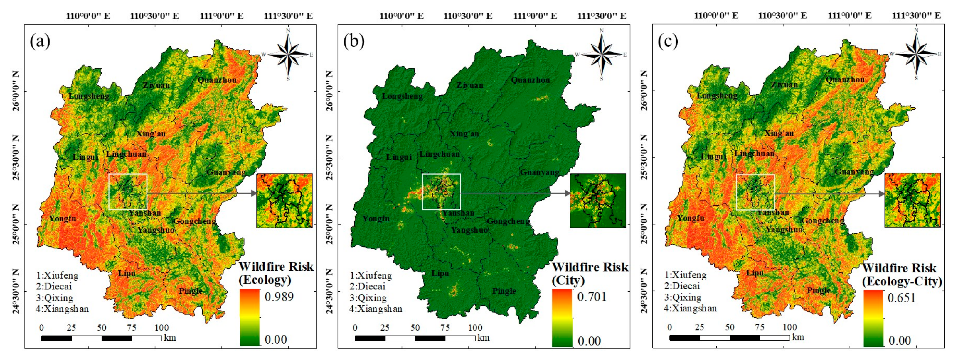
In this study, the wildfire susceptibility result of Guilin was synthesized with the wildfire vulnerability results of three dimensions of ecological environment, urban development and ecological–urban coupling using equation (30) to construct the corresponding wildfire riskiness model, and the results of the wildfire riskiness assessment are shown in Figure 19.
Regarding the ecological environment, the average wildfire risk in the study area is 0.407 (∈[0.4,0.6]), indicating a moderate risk of wildfire damage to the overall ecological environment of Guilin. The overall ecological environment is relatively healthy, with minimal disturbance from wildfires. As for urban development, the average wildfire risk in the study area is 0.003, indicating a low risk of wildfire damage to the overall urban development of Guilin. High-risk areas are mainly distributed in (1) the transitional zones between high-level urban areas such as Xiufeng, Diecai, Xiangshan, Qixing, and Lingui districts and surrounding forest areas, and (2) rural areas adjacent to forest areas with high vegetation cover and relatively high urbanization levels. Considering both the ecological environment and urban development, the average wildfire risk in the study area is 0.205, indicating a relatively low impact and destructive force of wildfires on Guilin overall. Compared with the respective risks of wildfires to the ecological and urban aspects, the integration of wildfire susceptibility and the vulnerability of the ecological–urban coupling has increased the risk in the surrounding urban areas and decreased the wildfire risk in non-urban areas. This makes the wildfire risk assessment more refined and reasonable, providing a good foundation for the sustainable development of Guilin and the protection of its ecological environment.

5. Discussion

5.1. Influence of Sample Confidence on Susceptibility Modeling Results

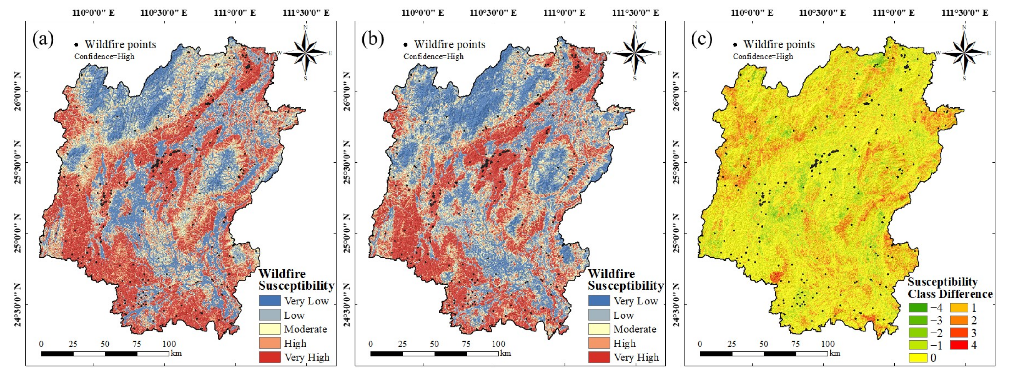
Compared with other wildfire products, active fire products such as VIIRS and MODIS not only possess excellent predictive accuracy but also have the ability to better identify wildfires occurring within small areas [100,101]. However, most current studies on wildfire susceptibility are based on selecting samples according to different criteria, with the most common method being the selection of high-confidence samples [12,102]. However, there are only 386 high-confidence wildfire samples within the study area from 2013 to 2022, and this number only represents the surface area covered by monitored wildfires, not the frequency of wildfire occurrence. Therefore, to ensure the reliability and completeness of the final wildfire susceptibility evaluation results, we selected 8791 samples with high- and nominal-confidence levels to construct the wildfire susceptibility model. Among them, nominal-confidence level refers to pixels that do not have potential solar flicker pollution during the day and are characterized by strong temperature anomalies (>15 K) in daytime or nighttime data.
To investigate the influence of sample confidence on the susceptibility modeling results, this study compared the optimal model in this article with the wildfire susceptibility model constructed using high-confidence samples. For the high-confidence model, the modeling method was consistent with that of this article: the XGBoost algorithm was selected, negative samples were randomly selected in non-wildfire areas with the same number as high-confidence samples, and the ratio of training set to test set was 7:3, with the same susceptibility classification standard. Figure 20 shows the wildfire susceptibility maps based on samples of different confidence intervals, as well as the difference maps of the zoning results between the two models. Through analysis, it was found that the average wildfire susceptibility values for the high-confidence sample-based susceptibility model and the optimal model in this article were 0.514 and 0.547, respectively. For the same evaluation unit, the former has an increased proportion of 16.523% of lower susceptibility regions and an increased proportion of 29.189% of higher susceptibility regions when compared with the latter, with an increase of 2.632% of high-confidence wildfire samples in the low susceptibility regions. Furthermore, the prediction accuracy of the susceptibility model based on high-confidence samples and the optimal model in this paper are 91.228% for high-confidence wildfire samples, and 97.458% and 98.305% for negative samples, respectively. It can be seen that the wildfire susceptibility model constructed by using both high- and nominal-confidence samples has higher prediction accuracy for reliable and accurate high-confidence wildfire samples, and has higher zonal rationality in the distribution of wildfire susceptibility areas.
The above results indicate that, based on qualified samples, using an ML algorithm to construct a wildfire susceptibility model in the city of Guilin with more data samples can not only improve the accuracy and robustness of the model, but also provide more opportunities to capture the trends and relationships between potential factors and wildfire occurrence, thereby reducing the risks of overfitting or underfitting. However, there is currently no good solution to ensure that samples have sufficient information coverage while screening highly reliable samples, which is also the focus of the next step of this research team’s work.

5.2. Comparison of ML Algorithms and Importance of Conditioning Factors

In recent years, ML algorithms have gained popularity for analyzing wildfire susceptibility by considering various environmental and human factors [7]. The main advantage of ML algorithms lies in their ability to handle complex and nonlinear relationships among input variables, which is particularly relevant in wildfire susceptibility modeling due to the intricate interactions among multiple factors leading to wildfires [15]. Several scholars have extensively studied the predictive performance of different ML algorithms on wildfire susceptibility in various regions. In our study, we evaluated the predictive performance of wildfire susceptibility in Guilin using both traditional ML algorithms (LR, ANN, KMM, SVM) and ensemble algorithms (XGBoost, LGBM, GBDT, RF). Our findings demonstrate that the ensemble algorithms (XGBoost, LGBM, GBDT, RF) outperformed the traditional ML algorithms. This conclusion aligns with the findings of other researchers [48,103,104,105,106]. Moreover, previous studies investigating wildfire susceptibility prediction, including the utilization of XGBoost, have also reported its strong performance [107,108,109,110].
Ensemble algorithms have been shown to effectively enhance the predictive performance of wildfire susceptibility compared to traditional ML algorithms. It is worth noting that there is no universally applicable ML algorithm in the field, and the selection of the most suitable algorithm depends on the specific region, task, and dataset. Therefore, different algorithms may exhibit varying predictive performance in different regions and datasets when studying wildfire susceptibility. Based on evaluation metrics such as AUC, accuracy, and RMSE, our study found that the XGBoost algorithm demonstrated the highest predictive performance in assessing wildfire susceptibility in Guilin.
Regarding the factors contributing to wildfire susceptibility in Guilin, our study identified temperature, soil type, land use, distance to roads, slope, and wind speed as the most significant contributors. Numerous studies have highlighted the prominent role of temperature in promoting wildfire occurrence [48,111], which aligns with our findings. However, some studies have suggested a minimal impact of temperature on wildfires [20,112]. Similarly, we found that land use type and distance to roads were important factors influencing wildfire occurrence [1,7,12,20]. The influence of slope as a significant topographical factor in wildfires is supported by extensive research [113,114]. Additionally, elevation, another recognized topographical factor, exhibited a moderate level of influence on wildfire susceptibility in our study. Consistent with prior research, higher wind speeds and lower rainfall were found to significantly increase wildfire susceptibility [48,115]. However, there are also studies suggesting the opposite, where lower wind speeds and higher rainfall lead to higher wildfire susceptibility [22].
It is evident that the analysis of wildfire conditioning factors’ importance may vary across regions and related studies. This variation can be attributed to differences in regional topography, climate, and human patterns, which shape the natural and social environmental factors and their influence on susceptibility. Moreover, variations in machine learning algorithms, their feature extraction methods, and data characteristics can contribute to discrepancies in factor importance rankings. Additionally, differences in datasets, including variations in data collection methods and the presence of outliers, can impact the interpretation of factor importance results.
Ensemble machine learning algorithms combine predictions from multiple weak learners to generate an ensemble prediction, effectively reducing the impact of outliers. This can be achieved through techniques such as voting or weighted averaging, improving prediction stability and accuracy. In parallel, the SHAP interpretability method, rooted in game theory, determines the importance of each feature by calculating their contribution to the prediction outcome, thereby addressing the issue of inconsistency in the way factor weights are evaluated in different algorithms. By employing a combination of ensemble algorithms and the SHAP method, more reliable results can be obtained in determining the importance of factors, enabling a deeper understanding and interpretation of the factors influencing wildfire susceptibility.

5.3. Comparison of SHAP Results between the Different Machine Learning Methods

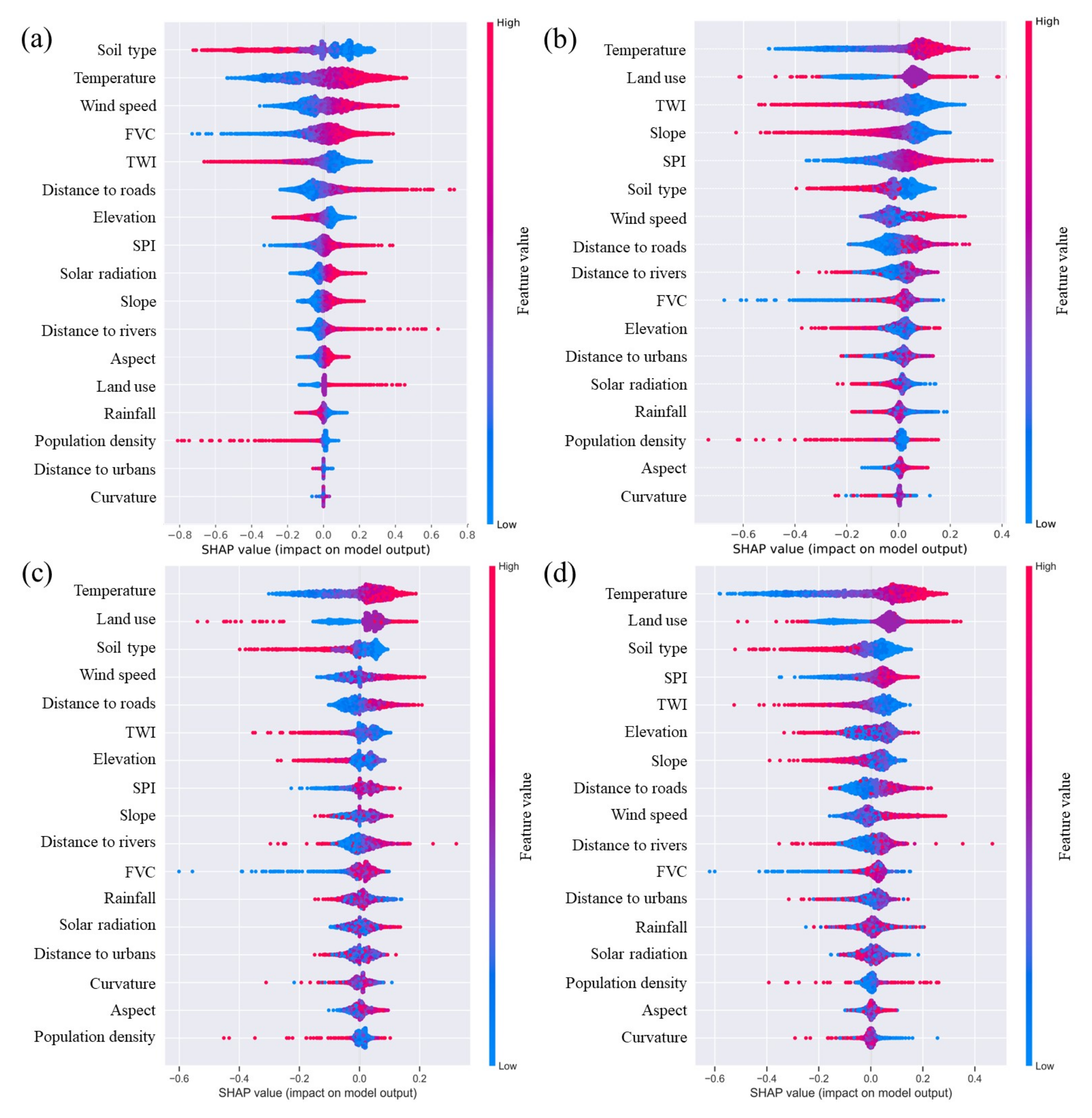
In our study, we used the SHAP method to investigate the effects and directions of various factors in different models on the prediction results, aiming to observe and evaluate the differences in their decision-making mechanisms. The summary SHAP plots for different models are shown in Figure 21 and Figure 22.
Among all the models, temperature was found to be the main influential factor, while aspect and curvature had relatively low impacts. However, the importance levels of other factors varied significantly among different models. In comparison to the ensemble models, traditional ML models (LR, ANN, KNN, SVM) showed a higher impact of TWI and SPI. In the LR model, FVC had a higher contribution, while land use had a lower contribution. In other models, land use generally had a higher contribution, while FVC had a moderate to lower contribution. Additionally, the directions of the effects of the same factor varied across different models. Solar radiation had a noticeable positive impact in the LR and KNN models, while it had a negative impact in the ANN model. In the four ensemble models (RF, GBDT, LGBM, and XGBoost) and the SVM model, the direction of its impact was not evident. Compared to traditional ML models, the same factor’s influence on the prediction results showed no significant differences in direction among the four ensemble models. Furthermore, although the relative importance of each factor varied among the different ensemble models, the fluctuations were relatively small. Temperature, soil type, and land use were found to be the most influential factors in terms of their contributions to the prediction results, while distance to roads, slope, and wind speed had slightly lower contributions compared to temperature, soil type, and land use. SPI, curvature, and aspect were identified as the factors with the least contribution to the model performance. The similarity in SHAP global interpretation results among the four ensemble models effectively validates the credibility of the susceptibility factor explanations results in our study.
It is noteworthy that this study merely employed SHAP to explain how various models, generated from the same factor data, predict wildfire susceptibility, rather than objectively explicate real-world principles. Furthermore, since this research was modeled based on specific sample data, alterations and modifications in any factor or sample may cause changes in the final wildfire susceptibility decision. Thus, SHAP is not essentially a simple causal model. To approach an objective reality in explaining the results of wildfire susceptibility models, not only must models with excellent performance be selected, but also the accuracy of sample data and the integrity of adjusted factors should be ensured.

5.4. Assessment Results of Wildfires in Each District and County

To better understand the comprehensive evaluation results of wildfire in various districts and counties of the city of Guilin, we calculated the average values of wildfire susceptibility, coupled with ecological environment and urban development wildfire vulnerability, and the corresponding wildfire risk within all grids in each district and county, as shown in Figure 23. According to the detailed statistical results (Table 6), Yongfu County, the city of Lipu, Lingchuan County, Xing’an County, Pingle County, Gongcheng County, and Lingui District have susceptibility values greater than 0.50, making them high-susceptibility areas for wildfire disasters in Guilin. Compared to the other 14 districts and counties, Xiufeng District, Qixing District, Xiangshan District, and Diecai District have a higher level of urban development while also possessing a good ecological environment, making them highly vulnerable areas for wildfire disasters in Guilin.
The relative differences in the levels of risk and susceptibility to wildfire disasters among various regions show remarkable similarity, with a high correlation coefficient of R2 = 0.947, indicating that wildfire susceptibility plays a significant role in disaster risk assessment. Among them, Yongfu County, Lipu City, Lingui District, and Pingle County exhibit higher levels of wildfire risk compared to other areas, posing a greater degree of risk in terms of destructive consequences and losses (such as human casualties, environmental damage, and economic losses) in the event of wildfire occurrence. In conclusion, a comprehensive evaluation of wildfire risk should take into account both the degree of wildfire susceptibility and coupled ecological and urban vulnerability, in order to gain a more comprehensive understanding of the likelihood, severity, and extent of wildfire occurrence. In addition, based on the key areas for wildfire prevention and control, planning and adjustment can be made in emergency response plans and resource allocation to improve the effectiveness of wildfire prevention and control.

6. Conclusions

This study presents a wildfire disaster assessment framework that aims to comprehensively analyze the law of wildfire susceptibility and the factors behind it, and to assess the risk of wildfires causing damage to local ecological environments and urban development. The study area selected for this study is Guilin, which has extremely high forest coverage. Multiple dimensions were used to assess and analyze wildfire susceptibility and potential losses. Firstly, based on 10 years of wildfire sample data, susceptibility conditioning factors were selected from topographical, surface environmental, anthropological, and meteorological aspects, and four traditional machine learning algorithms (LR, ANN, KNN, and SVR) and four ensemble algorithms (RF, GBDT, LGBM, and XGBoost) were used to construct a wildfire susceptibility model. The performance of the best model was explained, and feature analysis was conducted using the SHAP method, summarizing the occurrence and distribution characteristics of wildfires in Guilin. Secondly, by calculating the RSEI and NTLI, the ecological environment condition and urban development level of the region were evaluated, and the disaster vulnerability of the ecological environment, urban development, and the coupled ecological–urban disaster vulnerability were assessed. Finally, the best wildfire susceptibility model was combined with three dimensions of disaster vulnerability models to construct corresponding wildfire risk models, revealing the spatial distribution characteristics of the overall rules of wildfire disaster risk in Guilin. The research results indicate that
(1)
The ensemble models demonstrated superior predictive accuracy compared to traditional machine learning models. The XGBoost model achieved an AUC of 0.927 and accuracy of 0.863. High-susceptibility areas were found to be distributed in the central, northeast, south, and southwest regions of the study area, covering 41.758% of the entire region and encompassing 74.021% of wildfire samples. This model achieved the most reasonable susceptibility zoning results and the best predictive performance, making it the optimal model.
(2)
By using SHAP to interpret the results of the optimal model, the impact and intensity of each factor on wildfire occurrence in the study area were identified. The effects of changes in each factor on wildfire occurrence in the region were also explored. The factors that contributed the most to wildfire occurrence were found to be temperature, soil type, land use, distance to roads, slope, wind speed, distance to rivers, elevation, and FVC.
(3)
The ecological environment in the south, west, and northeast of Guilin was found to be vulnerable, while the urban development of Xiufeng, Diecai, Xiangshan, and Qixing districts and their surrounding counties was also found to be vulnerable. Furthermore, the vulnerability model that comprehensively considered ecology and urban development covered more high-vulnerability areas, more accurately divided low-vulnerability and high-vulnerability areas and provided richer detailed information.
(4)
From the perspectives of both ecological environment and urban development, potential wildfire risk areas can be identified and evaluated in a more targeted manner. However, a comprehensive evaluation that considers both aspects can provide a more holistic assessment of the wildfire disasters risk to human survival and environmental damage. This approach can enhance the comprehensiveness and accuracy of wildfire risk assessment and serve as a scientific basis for wildfire prevention and control.
Unlike most previous studies that only focused on improving model predictive accuracy to assess wildfire susceptibility, this study systematically assessed the patterns of susceptibility factors on wildfires, as well as the losses and potential threats of wildfires to the ecological environment and urban development. This research provided new insights for the assessment and study of regional wildfire disasters. The data used in this study can be obtained free of charge from relevant departments and channels and is applicable to other regions for wildfire disaster assessment research. Future research on wildfire-related studies aims to investigate the differences and patterns in wildfire susceptibility and risk distribution between northern and southern regions of China under varying spatiotemporal conditions, while effectively enhancing the reliability and precision of sample data and evaluation factors.

Author Contributions

Conceptualization, W.Y. and C.R.; methodology, W.Y. and C.R.; validation, W.Y. and C.R.; formal analysis, W.Y.; resources, W.Y. and C.R.; data curation, W.Y., C.R. and X.L.; writing original draft preparation, W.Y.; writing—review and editing, W.Y., C.R., Y.L. and J.L.; visualization, W.Y. and Z.W.; supervision, A.Y. and Y.L. and funding acquisition, A.Y. and Y.L. All authors have read and agreed to the published version of the manuscript.

Funding

This work was supported by the National Natural Science Foundation of China (Grant No. 42064003); Guangxi Natural Science Foundation (Grant No. 2021GXNSFBA220046).

Data Availability Statement

The hotspot datasets from 2013 to 2022 utilized in this study are freely available from the Fire In-formation for Resource Management System (FIRMS) at https://firms.modaps.eosdis.nasa.gov/ (accessed on 15 February 2023). Information on roads, buildings, and rivers can be obtained from the National Catalogue Service for Geographic Information (in Chinese) at https://www.webmap.cn/ (accessed on 15 February 2023). Land use type data is sourced from GlobeLand30 (in Chinese) at http://www.globallandcover.com/ (accessed on 15 February 2023). Population density information is obtained from the WorldPop Open Population Repository (WOPR) at https://hub.worldpop.org/ (accessed on 17 February 2023). Soil type data is obtained from the Harmonized World Soil Database (HWSD) at https://www.fao.org/soils-portal/data-hub/soil-maps-and-databases/harmonized-world-soil-database-v12/en/ (accessed on 17 February 2023). All other data are sourced from Google Earth Engine (GEE) at https://code.earthengine.google.com/ (accessed on 19 February 2023).

Conflicts of Interest

The authors declare no conflict of interest.

References

  1. Hong, H.; Jaafari, A.; Zenner, E.K. Predicting spatial patterns of wildfire susceptibility in the Huichang County, China: An integrated model to analysis of landscape indicators. Ecol. Indic. 2019, 101, 878–891. [Google Scholar] [CrossRef]
  2. Sachdeva, S.; Bhatia, T.; Verma, A. GIS-based evolutionary optimized Gradient Boosted Decision Trees for forest fire susceptibility mapping. Nat. Hazards 2018, 92, 1399–1418. [Google Scholar] [CrossRef]
  3. Pourghasemi, H.R.; Gayen, A.; Lasaponara, R.; Tiefenbacher, J.P. Application of learning vector quantization and different machine learning techniques to assessing forest fire influence factors and spatial modelling. Environ. Res. 2020, 184, 109321. [Google Scholar] [CrossRef] [PubMed]
  4. Zhang, G.; Wang, M.; Liu, K. Forest fire susceptibility modeling using a convolutional neural network for Yunnan province of China. Int. J. Disaster Risk Sci. 2019, 10, 386–403. [Google Scholar] [CrossRef]
  5. Gerdzheva, A.A. A comparative analysis of different wildfire risk assessment models (A case study for Smolyan district, Bulgaria). Eur. J. Geogr. 2014, 5, 22–36. [Google Scholar]
  6. Bui, D.T.; Hoang, N.-D.; Samui, P. Spatial pattern analysis and prediction of forest fire using new machine learning approach of Multivariate Adaptive Regression Splines and Differential Flower Pollination optimization: A case study at Lao Cai province (Viet Nam). J. Environ. Manag. 2019, 237, 476–487. [Google Scholar]
  7. Achu, A.; Thomas, J.; Aju, C.; Gopinath, G.; Kumar, S.; Reghunath, R. Machine-learning modelling of fire susceptibility in a forest-agriculture mosaic landscape of southern India. Ecol. Inform. 2021, 64, 101348. [Google Scholar] [CrossRef]
  8. Eskandari, S.; Miesel, J.R. Comparison of the fuzzy AHP method, the spatial correlation method, and the Dong model to predict the fire high-risk areas in Hyrcanian forests of Iran. Geomat. Nat. Hazards Risk 2017, 8, 933–949. [Google Scholar] [CrossRef]
  9. Al-Fugara, A.k.; Mabdeh, A.N.; Ahmadlou, M.; Pourghasemi, H.R.; Al-Adamat, R.; Pradhan, B.; Al-Shabeeb, A.R. Wildland fire susceptibility mapping using support vector regression and adaptive neuro-fuzzy inference system-based whale optimization algorithm and simulated annealing. ISPRS Int. J. Geo-Inf. 2021, 10, 382. [Google Scholar] [CrossRef]
  10. Tavakkoli Piralilou, S.; Einali, G.; Ghorbanzadeh, O.; Nachappa, T.G.; Gholamnia, K.; Blaschke, T.; Ghamisi, P. A Google Earth Engine approach for wildfire susceptibility prediction fusion with remote sensing data of different spatial resolutions. Remote Sens. 2022, 14, 672. [Google Scholar] [CrossRef]
  11. Bui, D.T.; Bui, Q.-T.; Nguyen, Q.-P.; Pradhan, B.; Nampak, H.; Trinh, P.T. A hybrid artificial intelligence approach using GIS-based neural-fuzzy inference system and particle swarm optimization for forest fire susceptibility modeling at a tropical area. Agric. For. Meteorol. 2017, 233, 32–44. [Google Scholar]
  12. Nur, A.S.; Kim, Y.J.; Lee, J.H.; Lee, C.-W. Spatial Prediction of Wildfire Susceptibility Using Hybrid Machine Learning Models Based on Support Vector Regression in Sydney, Australia. Remote Sens. 2023, 15, 760. [Google Scholar] [CrossRef]
  13. Nami, M.; Jaafari, A.; Fallah, M.; Nabiuni, S. Spatial prediction of wildfire probability in the Hyrcanian ecoregion using evidential belief function model and GIS. Int. J. Environ. Sci. Technol. 2018, 15, 373–384. [Google Scholar] [CrossRef]
  14. Salavati, G.; Saniei, E.; Ghaderpour, E.; Hassan, Q.K. Wildfire risk forecasting using weights of evidence and statistical index models. Sustainability 2022, 14, 3881. [Google Scholar] [CrossRef]
  15. Yuan, X.; Liu, C.; Nie, R.; Yang, Z.; Li, W.; Dai, X.; Cheng, J.; Zhang, J.; Ma, L.; Fu, X. A Comparative Analysis of Certainty Factor-Based Machine Learning Methods for Collapse and Landslide Susceptibility Mapping in Wenchuan County, China. Remote Sens. 2022, 14, 3259. [Google Scholar] [CrossRef]
  16. Cao, X.; Cui, X.; Yue, M.; Chen, J.; Tanikawa, H.; Ye, Y. Evaluation of wildfire propagation susceptibility in grasslands using burned areas and multivariate logistic regression. Int. J. Remote Sens. 2013, 34, 6679–6700. [Google Scholar] [CrossRef]
  17. Dutta, R.; Das, A.; Aryal, J. Big data integration shows Australian bush-fire frequency is increasing significantly. R. Soc. Open Sci. 2016, 3, 150241. [Google Scholar] [CrossRef]
  18. Ghorbanzadeh, O.; Valizadeh Kamran, K.; Blaschke, T.; Aryal, J.; Naboureh, A.; Einali, J.; Bian, J. Spatial prediction of wildfire susceptibility using field survey gps data and machine learning approaches. Fire 2019, 2, 43. [Google Scholar] [CrossRef]
  19. Arpaci, A.; Malowerschnig, B.; Sass, O.; Vacik, H. Using multi variate data mining techniques for estimating fire susceptibility of Tyrolean forests. Appl. Geogr. 2014, 53, 258–270. [Google Scholar] [CrossRef]
  20. He, Q.; Jiang, Z.; Wang, M.; Liu, K. Landslide and wildfire susceptibility assessment in southeast asia using ensemble machine learning methods. Remote Sens. 2021, 13, 1572. [Google Scholar] [CrossRef]
  21. Lan, Y.; Wang, J.; Hu, W.; Kurbanov, E.; Cole, J.; Sha, J.; Jiao, Y.; Zhou, J. Spatial pattern prediction of forest wildfire susceptibility in Central Yunnan Province, China based on multivariate data. Nat. Hazards 2022, 116, 565–586. [Google Scholar] [CrossRef]
  22. Abdollahi, A.; Pradhan, B. Explainable artificial intelligence (XAI) for interpreting the contributing factors feed into the wildfire susceptibility prediction model. Sci. Total Environ. 2023, 879, 163004. [Google Scholar] [CrossRef] [PubMed]
  23. Arrieta, A.B.; Díaz-Rodríguez, N.; Del Ser, J.; Bennetot, A.; Tabik, S.; Barbado, A.; García, S.; Gil-López, S.; Molina, D.; Benjamins, R. Explainable Artificial Intelligence (XAI): Concepts, taxonomies, opportunities and challenges toward responsible AI. Inf. Fusion 2020, 58, 82–115. [Google Scholar] [CrossRef]
  24. Cheng, X.; Wang, J.; Li, H.; Zhang, Y.; Wu, L.; Liu, Y. A method to evaluate task-specific importance of spatio-temporal units based on explainable artificial intelligence. Int. J. Geogr. Inf. Sci. 2021, 35, 2002–2025. [Google Scholar] [CrossRef]
  25. Lundberg, S.M.; Erion, G.G.; Lee, S.-I. Consistent individualized feature attribution for tree ensembles. arXiv 2018, arXiv:1802.03888. [Google Scholar]
  26. Dahal, A.; Lombardo, L. Explainable artificial intelligence in geoscience: A glimpse into the future of landslide susceptibility modeling. Comput. Geosci. 2023, 176, 105364. [Google Scholar] [CrossRef]
  27. Pradhan, B.; Lee, S.; Dikshit, A.; Kim, H. Spatial flood susceptibility mapping using an explainable artificial intelligence (XAI) model. Geosci. Front. 2023, 14, 101625. [Google Scholar] [CrossRef]
  28. Jena, R.; Pradhan, B.; Gite, S.; Alamri, A.; Park, H.-J. A new method to promptly evaluate spatial earthquake probability mapping using an explainable artificial intelligence (XAI) model. Gondwana Res. 2022; in press. [Google Scholar] [CrossRef]
  29. Iban, M.C.; Bilgilioglu, S.S. Snow avalanche susceptibility mapping using novel tree-based machine learning algorithms (XGBoost, NGBoost, and LightGBM) with eXplainable Artificial Intelligence (XAI) approach. Stoch. Environ. Res. Risk Assess. 2023, 37, 2243–2270. [Google Scholar] [CrossRef]
  30. Vaillant, N.M.; Kolden, C.A.; Smith, A.M. Assessing landscape vulnerability to wildfire in the USA. Curr. For. Rep. 2016, 2, 201–213. [Google Scholar] [CrossRef]
  31. Tang, X.; Machimura, T.; Li, J.; Yu, H.; Liu, W. Evaluating seasonal wildfire susceptibility and wildfire threats to local ecosystems in the largest forested area of China. Earth Future 2022, 10, e2021EF002199. [Google Scholar] [CrossRef]
  32. Ager, A.A.; Kline, J.D.; Fischer, A.P. Coupling the biophysical and social dimensions of wildfire risk to improve wildfire mitigation planning. Risk Anal. 2015, 35, 1393–1406. [Google Scholar] [CrossRef] [PubMed]
  33. Lan, Y.; Chen, J.; Yang, Y.; Ling, M.; You, H.; Han, X. Landscape Pattern and Ecological Risk Assessment in Guilin Based on Land Use Change. Int. J. Environ. Res. Public Health 2023, 20, 2045. [Google Scholar] [CrossRef] [PubMed]
  34. Liu, T.; Ren, C.; Zhang, S.; Yin, A.; Yue, W. Coupling Coordination Analysis of Urban Development and Ecological Environment in Urban Area of Guilin Based on Multi-Source Data. Int. J. Environ. Res. Public Health 2022, 19, 12583. [Google Scholar] [CrossRef]
  35. Trucchia, A.; Meschi, G.; Fiorucci, P.; Gollini, A.; Negro, D. Defining wildfire susceptibility maps in Italy for understanding seasonal wildfire regimes at the national level. Fire 2022, 5, 30. [Google Scholar] [CrossRef]
  36. Cao, C.; De Luccia, F.J.; Xiong, X.; Wolfe, R.; Weng, F. Early on-orbit performance of the visible infrared imaging radiometer suite onboard the Suomi National Polar-Orbiting Partnership (S-NPP) satellite. IEEE Trans. Geosci. Remote Sens. 2013, 52, 1142–1156. [Google Scholar] [CrossRef]
  37. Boschetti, L.; Roy, D.P.; Giglio, L.; Huang, H.; Zubkova, M.; Humber, M.L. Global validation of the collection 6 MODIS burned area product. Remote Sens. Environ. 2019, 235, 111490. [Google Scholar] [CrossRef]
  38. Giglio, L.; Schroeder, W.; Hall, J.; Justice, C. MODIS Collection 6 Active Fire Product User’s Guide Revision B; University of Maryland: College Park, MD, USA, 2018. [Google Scholar]
  39. Eskandari, S.; Khoshnevis, M. Evaluating and mapping the fire risk in the forests and rangelands of Sirachal using fuzzy analytic hierarchy process and GIS. For. Res. Dev. 2020, 6, 219–245. [Google Scholar]
  40. Youssef, A.M.; Pourghasemi, H.R. Landslide susceptibility mapping using machine learning algorithms and comparison of their performance at Abha Basin, Asir Region, Saudi Arabia. Geosci. Front. 2021, 12, 639–655. [Google Scholar] [CrossRef]
  41. Fang, L.; Yang, J.; Zu, J.; Li, G.; Zhang, J. Quantifying influences and relative importance of fire weather, topography, and vegetation on fire size and fire severity in a Chinese boreal forest landscape. For. Ecol. Manag. 2015, 356, 2–12. [Google Scholar] [CrossRef]
  42. Jaafari, A.; Pourghasemi, H.R. Factors Influencing Regional-Scale Wildfire Probability in Iran: An Application of Random Forest and Support Vector Machine. In Spatial Modeling in GIS and R for EARTH and Environmental Sciences; Elsevier: Amsterdam, The Netherlands, 2019; pp. 607–619. [Google Scholar]
  43. Lee, S.-W.; Won, M.-S.; Lee, J.-M.; Kim, H.-G. Intermediate-scale analysis of landscape characteristics affecting edge formation in burned forests in Samcheok, Korea. J. Mt. Sci. 2014, 11, 384–397. [Google Scholar] [CrossRef]
  44. Chuvieco, E.; Salas, J. Mapping the spatial distribution of forest fire danger using GIS. Int. J. Geogr. Inf. Sci. 1996, 10, 333–345. [Google Scholar] [CrossRef]
  45. Nguyen, Q.-H.; Chou, T.-Y.; Yeh, M.-L.; Hoang, T.-V.; Nguyen, H.-D.; Bui, Q.-T. Henry’s gas solubility optimization algorithm in formulating deep neural network for landslide susceptibility assessment in mountainous areas. Environ. Earth Sci. 2021, 80, 414. [Google Scholar] [CrossRef]
  46. Forkel, M.; Andela, N.; Harrison, S.P.; Lasslop, G.; Van Marle, M.; Chuvieco, E.; Dorigo, W.; Forrest, M.; Hantson, S.; Heil, A. Emergent relationships with respect to burned area in global satellite observations and fire-enabled vegetation models. Biogeosciences 2019, 16, 57–76. [Google Scholar] [CrossRef]
  47. Tonini, M.; D’Andrea, M.; Biondi, G.; Degli Esposti, S.; Trucchia, A.; Fiorucci, P. A machine learning-based approach for wildfire susceptibility mapping. The case study of the Liguria region in Italy. Geosciences 2020, 10, 105. [Google Scholar] [CrossRef]
  48. Iban, M.C.; Sekertekin, A. Machine learning based wildfire susceptibility mapping using remotely sensed fire data and GIS: A case study of Adana and Mersin provinces, Turkey. Ecol. Inform. 2022, 69, 101647. [Google Scholar] [CrossRef]
  49. Eskandari, S.; Pourghasemi, H.R.; Tiefenbacher, J.P. Fire-susceptibility mapping in the natural areas of Iran using new and ensemble data-mining models. Environ. Sci. Pollut. Res. 2021, 28, 47395–47406. [Google Scholar] [CrossRef]
  50. Cyr, D.; Gauthier, S.; Bergeron, Y. Scale-dependent determinants of heterogeneity in fire frequency in a coniferous boreal forest of eastern Canada. Landsc. Ecol. 2007, 22, 1325–1339. [Google Scholar] [CrossRef]
  51. Thach, N.N.; Ngo, D.B.-T.; Xuan-Canh, P.; Hong-Thi, N.; Thi, B.H.; Nhat-Duc, H.; Dieu, T.B. Spatial pattern assessment of tropical forest fire danger at Thuan Chau area (Vietnam) using GIS-based advanced machine learning algorithms: A comparative study. Ecol. Inform. 2018, 46, 74–85. [Google Scholar] [CrossRef]
  52. Xu, H. A remote sensing index for assessment of regional ecological changes. China Environ. Sci. 2013, 33, 889–897. [Google Scholar]
  53. Zheng, Z.; Wu, Z.; Chen, Y.; Yang, Z.; Marinello, F. Exploration of eco-environment and urbanization changes in coastal zones: A case study in China over the past 20 years. Ecol. Indic. 2020, 119, 106847. [Google Scholar] [CrossRef]
  54. Li, X.; Li, D.; Xu, H.; Wu, C. Intercalibration between DMSP/OLS and VIIRS Night-Time Light Images to Evaluate City Light Dynamics of Syria’s Major Human Settlement during Syrian Civil War. In Remote Sensing of Night-Time Light; Routledge: Oxford, UK, 2021; pp. 80–97. [Google Scholar]
  55. Zhu, Q.; Guo, X.; Guo, J.; Wu, J.; Ye, Y.; Cai, W.; Liu, S. The quality attribute of watershed ecosystem is more important than the landscape attribute in controlling erosion of red soil in southern China. Int. Soil Water Conserv. Res. 2022, 10, 507–517. [Google Scholar] [CrossRef]
  56. Lobser, S.; Cohen, W. MODIS tasselled cap: Land cover characteristics expressed through transformed MODIS data. Int. J. Remote Sens. 2007, 28, 5079–5101. [Google Scholar] [CrossRef]
  57. Chander, G.; Markham, B.L.; Helder, D.L. Summary of current radiometric calibration coefficients for Landsat MSS, TM, ETM+, and EO-1 ALI sensors. Remote Sens. Environ. 2009, 113, 893–903. [Google Scholar] [CrossRef]
  58. Cui, H.; Qiu, S.; Wang, Y.; Zhang, Y.; Liu, Z.; Karila, K.; Jia, J.; Chen, Y. Disaster-Caused Power Outage Detection at Night Using VIIRS DNB Images. Remote Sens. 2023, 15, 640. [Google Scholar] [CrossRef]
  59. Gao, S.; Chen, Y.; Liang, L.; Gong, A. Post-earthquake night-time light piecewise (PNLP) pattern based on NPP/VIIRS night-time light data: A case study of the 2015 Nepal earthquake. Remote Sens. 2020, 12, 2009. [Google Scholar] [CrossRef]
  60. Chen, X.; Chen, W. GIS-based landslide susceptibility assessment using optimized hybrid machine learning methods. Catena 2021, 196, 104833. [Google Scholar] [CrossRef]
  61. Zhao, X.; Chen, W. Optimization of computational intelligence models for landslide susceptibility evaluation. Remote Sens. 2020, 12, 2180. [Google Scholar] [CrossRef]
  62. Jaafari, A.; Zenner, E.K.; Pham, B.T. Wildfire spatial pattern analysis in the Zagros Mountains, Iran: A comparative study of decision tree based classifiers. Ecol. Inform. 2018, 43, 200–211. [Google Scholar] [CrossRef]
  63. Tang, X.; Machimura, T.; Li, J.; Liu, W.; Hong, H. A novel optimized repeatedly random undersampling for selecting negative samples: A case study in an SVM-based forest fire susceptibility assessment. J. Environ. Manag. 2020, 271, 111014. [Google Scholar] [CrossRef]
  64. Chen, W.; Li, Y.; Xue, W.; Shahabi, H.; Li, S.; Hong, H.; Wang, X.; Bian, H.; Zhang, S.; Pradhan, B. Modeling flood susceptibility using data-driven approaches of naïve bayes tree, alternating decision tree, and random forest methods. Sci. Total Environ. 2020, 701, 134979. [Google Scholar] [CrossRef] [PubMed]
  65. Pham, B.T.; Prakash, I.; Jaafari, A.; Bui, D.T. Spatial prediction of rainfall-induced landslides using aggregating one-dependence estimators classifier. J. Indian Soc. Remote Sens. 2018, 46, 1457–1470. [Google Scholar] [CrossRef]
  66. Zhang, G.; Patuwo, B.E.; Hu, M.Y. Forecasting with artificial neural networks: The state of the art. Int. J. Forecast. 1998, 14, 35–62. [Google Scholar] [CrossRef]
  67. Safi, Y.; Bouroumi, A. Prediction of forest fires using artificial neural networks. Appl. Math. Sci. 2013, 7, 271–286. [Google Scholar] [CrossRef]
  68. Cover, T.; Hart, P. Nearest neighbor pattern classification. IEEE Trans. Inf. Theory 1967, 13, 21–27. [Google Scholar] [CrossRef]
  69. He, Q.P.; Wang, J. Fault detection using the k-nearest neighbor rule for semiconductor manufacturing processes. IEEE Trans. Semicond. Manuf. 2007, 20, 345–354. [Google Scholar] [CrossRef]
  70. Noble, W.S. What is a support vector machine? Nat. Biotechnol. 2006, 24, 1565–1567. [Google Scholar] [CrossRef]
  71. Rigatti, S.J. Random forest. J. Insur. Med. 2017, 47, 31–39. [Google Scholar] [CrossRef]
  72. Qi, M.L. A Highly Efficient Gradient Boosting Decision Tree [C]. In Neural Information Processing Systems; Curran Associates Inc.: Red Hook, NY, USA, 2017. [Google Scholar]
  73. Sachdeva, S.; Kumar, B. Comparison of gradient boosted decision trees and random forest for groundwater potential mapping in Dholpur (Rajasthan), India. Stoch. Environ. Res. Risk Assess 2021, 35, 287–306. [Google Scholar] [CrossRef]
  74. Aziz, R.M.; Baluch, M.F.; Patel, S.; Ganie, A.H. LGBM: A machine learning approach for Ethereum fraud detection. Int. J. Inf. Technol. 2022, 14, 3321–3331. [Google Scholar] [CrossRef]
  75. Chen, T.; Guestrin, C. Xgboost: A Scalable Tree Boosting System. In Proceedings of the 22nd Acm Sigkdd International Conference on Knowledge Discovery and Data Mining, San Francisco, CA, USA, 13–17 August 2016; pp. 785–794. [Google Scholar]
  76. Fan, J.; Wang, X.; Wu, L.; Zhou, H.; Zhang, F.; Yu, X.; Lu, X.; Xiang, Y. Comparison of Support Vector Machine and Extreme Gradient Boosting for predicting daily global solar radiation using temperature and precipitation in humid subtropical climates: A case study in China. Energy Convers. Manag. 2018, 164, 102–111. [Google Scholar] [CrossRef]
  77. Merghadi, A.; Yunus, A.P.; Dou, J.; Whiteley, J.; ThaiPham, B.; Bui, D.T.; Avtar, R.; Abderrahmane, B. Machine learning methods for landslide susceptibility studies: A comparative overview of algorithm performance. Earth-Sci. Rev. 2020, 207, 103225. [Google Scholar] [CrossRef]
  78. Ling, C.X.; Huang, J.; Zhang, H. AUC: A Better Measure than Accuracy in Comparing Learning Algorithms. In Proceedings of the Advances in Artificial Intelligence: 16th Conference of the Canadian Society for Computational Studies of Intelligence, AI 2003, Halifax, NS, Canada, 11–13 June 2003; pp. 329–341. [Google Scholar]
  79. Tekin, S.; Çan, T. Slide type landslide susceptibility assessment of the Büyük Menderes watershed using artificial neural network method. Environ. Sci. Pollut. Res. 2022, 29, 47174–47188. [Google Scholar] [CrossRef] [PubMed]
  80. Bradley, A.P. The use of the area under the ROC curve in the evaluation of machine learning algorithms. Pattern Recognit. 1997, 30, 1145–1159. [Google Scholar] [CrossRef]
  81. Panahi, M.; Sadhasivam, N.; Pourghasemi, H.R.; Rezaie, F.; Lee, S. Spatial prediction of groundwater potential mapping based on convolutional neural network (CNN) and support vector regression (SVR). J. Hydrol. 2020, 588, 125033. [Google Scholar] [CrossRef]
  82. Nhu, V.-H.; Shirzadi, A.; Shahabi, H.; Singh, S.K.; Al-Ansari, N.; Clague, J.J.; Jaafari, A.; Chen, W.; Miraki, S.; Dou, J. Shallow landslide susceptibility mapping: A comparison between logistic model tree, logistic regression, naïve bayes tree, artificial neural network, and support vector machine algorithms. Int. J. Environ. Res. Public Health 2020, 17, 2749. [Google Scholar] [CrossRef] [PubMed]
  83. Lundberg, S.M.; Lee, S.-I. A Unified Approach to Interpreting Model Predictions. In Advances in Neural Information Processing Systems; Curran Associates Inc.: Red Hook, NY, USA, 2017; p. 30. [Google Scholar]
  84. Chen, S. Interpretation of multi-label classification models using shapley values. arXiv 2021, arXiv:2104.10505. [Google Scholar]
  85. Kavzoglu, T.; Teke, A.; Yilmaz, E.O. Shared blocks-based ensemble deep learning for shallow landslide susceptibility mapping. Remote Sens. 2021, 13, 4776. [Google Scholar] [CrossRef]
  86. Kannangara, K.P.M.; Zhou, W.; Ding, Z.; Hong, Z. Investigation of feature contribution to shield tunneling-induced settlement using Shapley additive explanations method. J. Rock Mech. Geotech. Eng. 2022, 14, 1052–1063. [Google Scholar] [CrossRef]
  87. Mangalathu, S.; Hwang, S.-H.; Jeon, J.-S. Failure mode and effects analysis of RC members based on machine-learning-based SHapley Additive exPlanations (SHAP) approach. Eng. Struct. 2020, 219, 110927. [Google Scholar] [CrossRef]
  88. DHA UN. Internationally Agreed Glossary of Basic Terms Related to Disaster Management; UN DHA (United Nations Dep. Humanit. Aff.): Geneva, Switzerland, 1992. [Google Scholar]
  89. Yue, H.; Liu, Y.; Li, Y.; Lu, Y. Eco-environmental quality assessment in China’s 35 major cities based on remote sensing ecological index. IEEE Access 2019, 7, 51295–51311. [Google Scholar] [CrossRef]
  90. Knight, F.H. Risk, Uncertainty and Profit; Houghton Mifflin: Boston, MA, USA, 1921; Volume 31. [Google Scholar]
  91. Jiménez-Perálvarez, J. Landslide-risk mapping in a developing hilly area with limited information on landslide occurrence. Landslides 2018, 15, 741–752. [Google Scholar] [CrossRef]
  92. Li, X.; Cheng, J.; Yu, D. Research on Landslide Risk Assessment Based on Convolutional Neural Network. IEEE Geosci. Remote Sens. Lett. 2022, 19, 2505705. [Google Scholar] [CrossRef]
  93. Scheuer, S.; Haase, D.; Meyer, V. Exploring multicriteria flood vulnerability by integrating economic, social and ecological dimensions of flood risk and coping capacity: From a starting point view towards an end point view of vulnerability. Nat. Hazards 2011, 58, 731–751. [Google Scholar] [CrossRef]
  94. Xiong, Y.; Zhou, Y.; Wang, F.; Wang, S.; Wang, Z.; Ji, J.; Wang, J.; Zou, W.; You, D.; Qin, G. A Novel Intelligent Method Based on the Gaussian Heatmap Sampling Technique and Convolutional Neural Network for Landslide Susceptibility Mapping. Remote Sens. 2022, 14, 2866. [Google Scholar] [CrossRef]
  95. García, M.V.; Aznarte, J.L. Shapley additive explanations for NO2 forecasting. Ecol. Inform. 2020, 56, 101039. [Google Scholar] [CrossRef]
  96. Cha, Y.; Shin, J.; Go, B.; Lee, D.-S.; Kim, Y.; Kim, T.; Park, Y.-S. An interpretable machine learning method for supporting ecosystem management: Application to species distribution models of freshwater macroinvertebrates. J. Environ. Manag. 2021, 291, 112719. [Google Scholar] [CrossRef]
  97. Sun, D.; Ding, Y.; Zhang, J.; Wen, H.; Wang, Y.; Xu, J.; Zhou, X.; Liu, R. Essential insights into decision mechanism of landslide susceptibility mapping based on different machine learning models. In Geocarto International; Taylor & Francis: Abingdon, UK, 2022; pp. 1–29. [Google Scholar]
  98. Ye, X.; Kuang, H. Evaluation of ecological quality in southeast Chongqing based on modified remote sensing ecological index. Sci. Rep. 2022, 12, 15694. [Google Scholar] [CrossRef]
  99. Tan, M. Use of an inside buffer method to extract the extent of urban areas from DMSP/OLS nighttime light data in North China. Giscience Remote Sens. 2016, 53, 444–458. [Google Scholar] [CrossRef]
  100. Schroeder, W.; Oliva, P.; Giglio, L.; Csiszar, I.A. The New VIIRS 375 m active fire detection data product: Algorithm description and initial assessment. Remote Sens. Environ. 2014, 143, 85–96. [Google Scholar] [CrossRef]
  101. Giglio, L.; Schroeder, W.; Justice, C.O. The collection 6 MODIS active fire detection algorithm and fire products. Remote Sens. Environ. 2016, 178, 31–41. [Google Scholar] [CrossRef]
  102. Wang, W.; Zhao, F.; Wang, Y.; Huang, X.; Ye, J. Seasonal differences in the spatial patterns of wildfire drivers and susceptibility in the southwest mountains of China. Sci. Total Environ. 2023, 869, 161782. [Google Scholar] [CrossRef] [PubMed]
  103. Gholamnia, K.; Gudiyangada Nachappa, T.; Ghorbanzadeh, O.; Blaschke, T. Comparisons of diverse machine learning approaches for wildfire susceptibility mapping. Symmetry 2020, 12, 604. [Google Scholar] [CrossRef]
  104. Pouyan, S.; Pourghasemi, H.R.; Bordbar, M.; Rahmanian, S.; Clague, J.J. A multi-hazard map-based flooding, gully erosion, forest fires, and earthquakes in Iran. Sci. Rep. 2021, 11, 14889. [Google Scholar] [CrossRef] [PubMed]
  105. Cao, Y.; Wang, M.; Liu, K. Wildfire susceptibility assessment in Southern China: A comparison of multiple methods. Int. J. Disaster Risk Sci. 2017, 8, 164–181. [Google Scholar] [CrossRef]
  106. Sun, Y.; Zhang, F.; Lin, H.; Xu, S. A Forest Fire Susceptibility Modeling Approach Based on Light Gradient Boosting Machine Algorithm. Remote Sens. 2022, 14, 4362. [Google Scholar] [CrossRef]
  107. Seddouki, M.; Benayad, M.; Aamir, Z.; Tahiri, M.; Maanan, M.; Rhinane, H. Using Machine Learning Coupled with Remote Sensing for Forest Fire Susceptibility Mapping. Case Study Tetouan Province, Northern Morocco. Int. Arch. Photogramm. Remote Sens. Spat. Inf. Sci. 2023, 48, 333–342. [Google Scholar] [CrossRef]
  108. Shmuel, A.; Heifetz, E. Global wildfire susceptibility mapping based on machine learning models. Forests 2022, 13, 1050. [Google Scholar] [CrossRef]
  109. Akıncı, H.A.; Akıncı, H. Machine learning based forest fire susceptibility assessment of Manavgat district (Antalya), Turkey. Earth Sci. Inform. 2023, 16, 397–414. [Google Scholar] [CrossRef]
  110. Abujayyab, S.K.; Kassem, M.M.; Khan, A.A.; Wazirali, R.; Coşkun, M.; Taşoğlu, E.; Öztürk, A.; Toprak, F. Wildfire Susceptibility Mapping Using Five Boosting Machine Learning Algorithms: The Case Study of the Mediterranean Region of Turkey. Adv. Civ. Eng. 2022, 2022, 3959150. [Google Scholar] [CrossRef]
  111. Yang, X.; Jin, X.; Zhou, Y. Wildfire risk assessment and zoning by integrating Maxent and GIS in Hunan province, China. Forests 2021, 12, 1299. [Google Scholar] [CrossRef]
  112. Hong, H.; Tsangaratos, P.; Ilia, I.; Liu, J.; Zhu, A.-X.; Xu, C. Applying genetic algorithms to set the optimal combination of forest fire related variables and model forest fire susceptibility based on data mining models. The case of Dayu County, China. Sci. Total Environ. 2018, 630, 1044–1056. [Google Scholar] [CrossRef] [PubMed]
  113. De Santana, R.O.; Delgado, R.C.; Schiavetti, A. Modeling susceptibility to forest fires in the Central Corridor of the Atlantic Forest using the frequency ratio method. J. Environ. Manag. 2021, 296, 113343. [Google Scholar] [CrossRef] [PubMed]
  114. Cilli, R.; Elia, M.; D’Este, M.; Giannico, V.; Amoroso, N.; Lombardi, A.; Pantaleo, E.; Monaco, A.; Sanesi, G.; Tangaro, S. Explainable artificial intelligence (XAI) detects wildfire occurrence in the Mediterranean countries of Southern Europe. Sci. Rep. 2022, 12, 16349. [Google Scholar] [CrossRef] [PubMed]
  115. Eskandari, S.; Miesel, J.R.; Pourghasemi, H.R. The temporal and spatial relationships between climatic parameters and fire occurrence in northeastern Iran. Ecol. Indic. 2020, 118, 106720. [Google Scholar] [CrossRef]
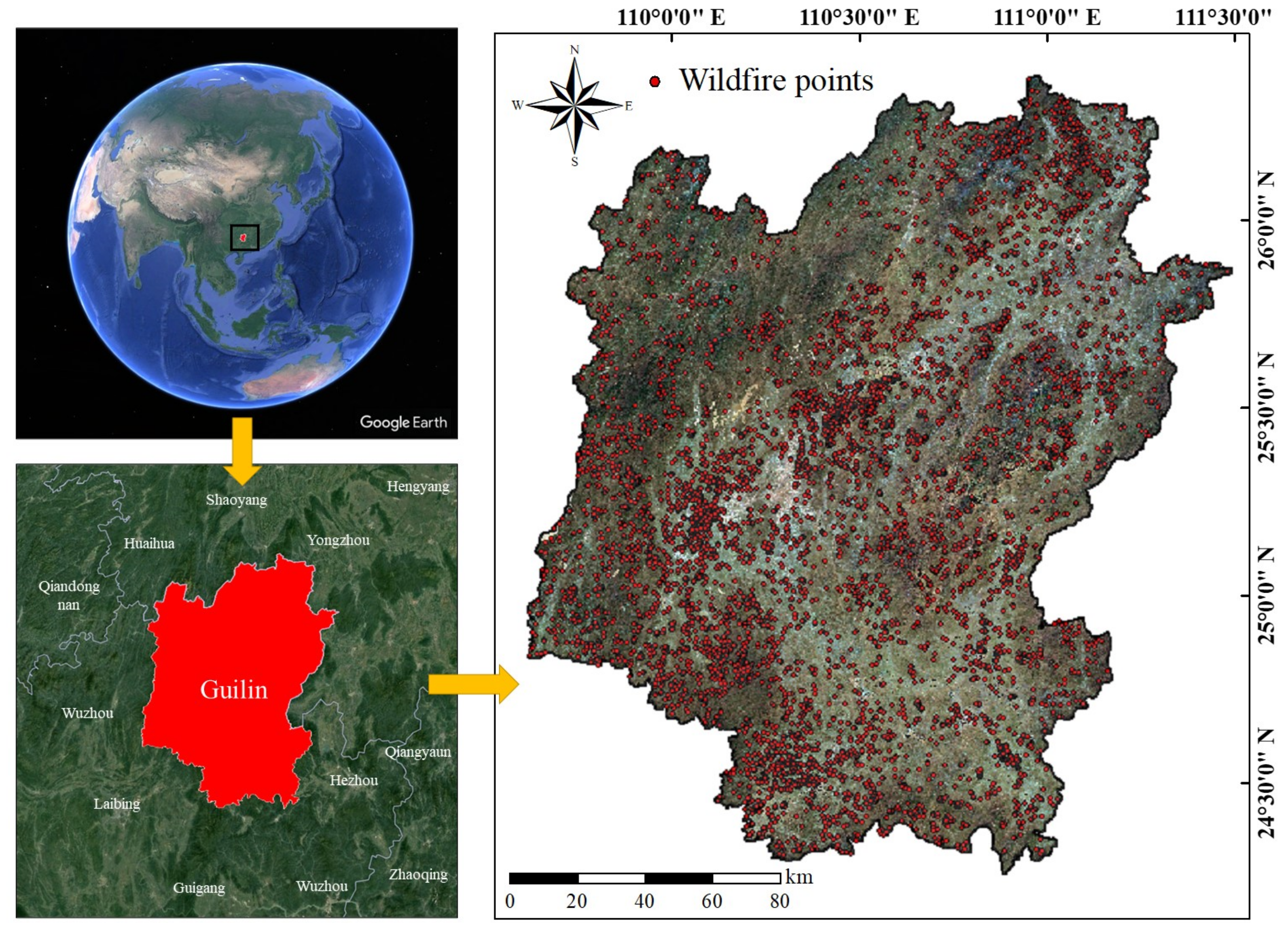
Figure 1. The location of the study area and the distribution of wildfire points.
Remotesensing 15 02659 g001
Figure 2. Maps of topographical conditioning factors: (a) elevation, (b) slope, (c) aspect, (d) curvature, (e) TWI, and (f) SPI.
Remotesensing 15 02659 g002
Figure 3. Maps of surface environmental conditioning factors: (a) FVC, (b) soil type, and (c) distance to rivers.
Remotesensing 15 02659 g003
Figure 4. Maps of anthropological conditioning factors: (a) land use, (b) population density, (c) distance to roads, and (d) distance to urban areas.
Remotesensing 15 02659 g004
Figure 5. Maps of meteorological conditioning factors: (a) rainfall, (b) solar radiation, (c) temperature, and (d) wind speed.
Remotesensing 15 02659 g005
Figure 6. Maps of ecological vulnerability factors: (a) NDVI, (b) NDBSI, (c) WET, and (d) LST.
Remotesensing 15 02659 g006
Figure 7. Maps of urban vulnerability factors: (a) before denoising, (b) after denoising.
Remotesensing 15 02659 g007
Figure 8. Flowchart of wildfire susceptibility assessment in Guilin.
Remotesensing 15 02659 g008
Figure 9. Flowchart of wildfire vulnerability assessment in Guilin.
Remotesensing 15 02659 g009
Figure 10. Wildfire susceptibility maps generated using different ML methods: (a) LR, (b) ANN, (c) KNN, and (d) SVR.
Remotesensing 15 02659 g010
Figure 11. Wildfire susceptibility maps generated using different ML methods: (a) RF, (b) GBDT, (c) LGBM, and (d) XGBoost.
Remotesensing 15 02659 g011
Figure 12. Statistical results of wildfire susceptibility zoning classes: (a) area proportion of each wildfire susceptibility level; (b) proportion of wildfire samples in each wildfire susceptibility level.
Remotesensing 15 02659 g012
Figure 13. Wildfire frequency ratio of each susceptibility level.
Remotesensing 15 02659 g013
Figure 14. ROC curve of each model.
Remotesensing 15 02659 g014
Figure 15. Wildfire conditioning factor ranking: (a) summary plot of Shapley values; (b) factor importance plot.
Remotesensing 15 02659 g015
Figure 16. Dependence plots of main factors: (a) temperature, (b) soil type, (c) land use, (d) distance to roads, (e) slope, (f) wind speed, (g) distance to rivers, (h) elevation, and (i) FVC.
Remotesensing 15 02659 g016
Figure 17. Local interpretation results of major historical disasters: (a) detailed map of wildfire susceptibility in Xing’an, (b) local interpretation plot of wildfire disaster in Xing’an, (c) detailed map of wildfire susceptibility in Quanzhou, (d) local interpretation plot of wildfire disaster in Quanzhou, (e) detailed map of wildfire susceptibility in Diecai, and (f) local interpretation plot of wildfire disaster in Diecai.
Remotesensing 15 02659 g017
Figure 18. Wildfire vulnerability maps: (a) ecology, (b) city, and (c) ecology–city coupling.
Remotesensing 15 02659 g018
Figure 19. Wildfire risk maps: (a) ecology, (b) city, and (c) ecology–city coupling.
Remotesensing 15 02659 g019
Figure 20. Wildfire susceptibility map based on samples with different confidence: (a) confidence = high, (b) confidence = high + nominal (optimal model in this paper), and (c) susceptibility class difference.
Remotesensing 15 02659 g020
Figure 21. Summary plot of Shapley values of different ML methods: (a) LR, (b) ANN, (c) KNN, and (d) SVM.
Remotesensing 15 02659 g021
Figure 22. Summary plot of Shapley values of different ML methods: (a) RF, (b) GBDT, (c) LGBM, and (d) XGBoost.
Remotesensing 15 02659 g022
Figure 23. Wildfire assessment map of each district and county: (a) susceptibility, (b) vulnerability, and (c) risk.
Remotesensing 15 02659 g023
Table 1. Information on susceptibility conditioning factors.
CategoryFactorsSource of DataFormat and Scale/ResolutionData Type
TopographicalElevationSRTM DEM30 m (.tiff)Numerical
SlopeNumerical
AspectCategorical
CurvatureNumerical
TWINumerical
SPINumerical
Surface
environmental
FVCLandsat 8 OLI (2013–2022)30 m (.tiff)Numerical
Soil typeHarmonized World Soil
Database (HWSD)
5′ (.tiff)Categorical
Distance to riversNational Catalogue Service for Geographic Information (in Chinese)1:250,000 (.shp)Numerical
AnthropologicalDistance to roadsNational Catalogue Service for Geographic Information (in Chinese)1:250,000 (.shp)Numerical
Distance to urban areas Numerical
Land useGlobeLand30 V2020 data
(in Chinese)
30 m (.tiff)Categorical
Population densityWorldPop dataset1 km (.tiff)Numerical
MeteorologicalRainfall (surface)ERA5-Land reanalysis dataset
(2013–2022)
11,132 m (.tiff)Numerical
Solar radiation (surface)Numerical
Temperature (2 m)Numerical
Wind speed (10 m)Numerical
Table 2. Hyperparameter tuning results for each algorithm.
AlgorithmHyperparametersValue
LRmax_iter
(The maximum number of iterations)
500
ANNunits
(the number of hidden layers activation)
9
“relu” and “sigmoid”
learning_rate0.001
KNNn_neighbors15
weights“distance”
SVRkernel function“rbf”
C4
gamma0.06
RFmax_features8
n_estimators500
max_depth10
GBDTn_estimators240
max_depth9
subsample0.9
LGBMn_estimators400
max_depth12
num_leaves90
min_child_samples3
colsample_bytree0.6
XGBoostn_estimators600
max_depth10
subsample0.9
min_child_weight3
colsample_bytree0.6
Table 3. Multiple collinearity analysis results of wildfire conditioning factors.
Conditioning FactorMulticollinearity Scores
TOLVIF
Elevation0.3043.287
Slope0.3482.878
Aspect0.9871.013
Curvature0.8451.184
TWI0.4192.389
SPI0.4622.164
Land use0.8011.248
Soil type0.9001.111
Population density0.8261.211
Distance to rivers0.9091.101
Distance to roads0.8521.174
Distance to urbans0.5781.731
FVC0.6961.437
Rainfall0.7991.252
Solar radiation0.7141.400
Temperature0.3372.964
Wind speed0.6411.560
Table 4. Predictive performance of each model.
ModelSensitivitySpecificityPrecisionF1-ScoreAccuracyRMSE (All)RMSE (1)RMSE (0)
LR0.7230.7460.7390.7310.7350.4230.4350.409
ANN0.7370.8910.8700.7980.8140.3720.4230.313
KNN0.7610.8530.8370.7970.8070.3690.3790.360
SVM0.7580.8830.8660.8090.8210.3720.4260.310
RF0.7880.9170.9040.8420.8530.3350.3630.305
GBDT0.8140.8910.8810.8460.8530.3330.3590.305
LGBM0.8180.8990.8900.8520.8590.3300.3580.301
XGBoost0.8180.9070.8980.8560.8630.3270.3560.294
Table 5. Information of historical major wildfire disasters in Guilin.
No.Wildfire Disaster SiteTimeLongitude/°Latitude/°
1Yijia Village, Rongjiang Town, Xing’an County2022.10.17 Day110.4489125.4925
2Baimao Village, Wenqiao Town, Quanzhou County2022.10.17 Day111.0827226.19362
3Yaoshan, Diecai District2019.12.6 Night110.36846925.303186
Table 6. Statistical results of wildfire assessment in each district and county.
District and CountySusceptibility ValueSusceptibility
Ranking
Vulnerability ValueVulnerability RankingRisk ValueRisk
Ranking
Xiufeng0.199170.49310.09816
Diecai0.45190.46140.1968
Xiangshan0.377120.46330.17111
Qixing0.300150.48120.13814
Yanshan0.361130.41570.15113
Lingui0.52170.41960.2193
Yangshuo0.442100.40780.18110
Lingchuan0.62230.386130.2145
Quanzhou0.49680.388120.1959
Xing’an0.55840.375160.2106
Yongfu0.76110.42350.3211
Guanyang0.420110.368170.15912
Longsheng0.317140.404100.13115
Ziyuan0.250160.376150.09617
Pingle0.54350.400110.2184
Lipu0.68520.40690.2772
Gongcheng0.52460.384140.2047
Whole region0.514-0.395-0.205-
Disclaimer/Publisher’s Note: The statements, opinions and data contained in all publications are solely those of the individual author(s) and contributor(s) and not of MDPI and/or the editor(s). MDPI and/or the editor(s) disclaim responsibility for any injury to people or property resulting from any ideas, methods, instructions or products referred to in the content.