Abstract
Landslides are a dangerous natural hazard that can critically harm road infrastructure in mountainous places, resulting in significant damage and fatalities. The primary purpose of this study was to assess the efficacy of three machine learning algorithms (MLAs) for landslide susceptibility mapping including random forest (RF), decision tree (DT), and support vector machine (SVM). We selected a case study region that is frequently affected by landslides, the important Kamyaran–Sarvabad road in the Kurdistan province of Iran. Altogether, 14 landslide evaluation factors were input into the MLAs including slope, aspect, elevation, river density, distance to river, distance to fault, fault density, distance to road, road density, land use, slope curvature, lithology, stream power index (SPI), and topographic wetness index (TWI). We identified 64 locations of landslides by field survey of which 70% were randomly employed for building and training the three MLAs while the remaining locations were used for validation. The area under the receiver operating characteristics (AUC) reached a value of 0.94 for the decision tree compared to 0.82 for the random forest, and 0.75 for support vector machines model. Thus, the decision tree model was most accurate in identifying the areas at risk for future landslides. The obtained results may inform geoscientists and those in decision-making roles for landslide management.
1. Introduction
A landslide is one of the most common and harmful geological disasters in the world, causing fatalities, property damage, and economic downturns [1]. Natural events and anthropogenic activities trigger landslides [2,3]. Many geoscience researchers have emphasised that because of the complexity of both natural and anthropogenic factors that are assumed to be accountable for the evaluation of landslides, it is difficult to predict the spatial and temporal occurrence of landslides [4,5]. These catastrophic occurrences caused a great quantity of fatalities, injuries, and infrastructure damage, especially of road networks [6,7]. Hence, 1.3% of fatalities in all natural disasters occurred from landslides, with Asia accounting for around 54% of these landslides [8].
Iran has always been prone to landslides. The Alborz Mountain and the Zagros Mountain both have a moderate to high susceptibility to landslides, with the Zagros Mountain being considerably more sensitive [9]. Landslides, especially in mountainous regions, have the potential to destroy roads and railroads and even result in fatalities [10]. Previous studies that created landslide susceptibility maps to indicate where landslides are most prone to occur [11] used a variety of statistical techniques [12,13,14]. Recently, machine learning algorithms (MLAs) have gained popularity among academics and industry professionals and have significantly improved geohazard modelling [15,16]. The large datasets of landslide susceptibility maps (LSMs) can be utilized by MLAs techniques such as support vector machine (SVM) [17], decision tree (DT), neuro-fuzzy systems, random forest (RF) [18], decision tree [19], kernel logistic regression (KLR) [20], random forest (RF) [21], and artificial neural networks (ANN) [22]. These techniques have enhanced precision and processing adaptability [23]. To enhance planning and control the risk of landslides, landslide susceptibility mapping can be utilized as a practical technique [24]. Landslides may occur or become more intense as a result of the construction of roads and communication lines in hilly terrain, as is the case for the road that we studied. It is therefore essential to use these algorithms to identify slope movements, the mechanisms causing them, as well as effective factors in slope instability.
To the best of our knowledge, the literature review shows that studies of natural hazards, including landslides, have been carried out by many researchers using various techniques and methods in many different regions of the world. However, this process has not stopped yet, and these studies are still ongoing because achieving a technique that can effectively detect landslide-prone areas, especially using satellite imagery and radar data, is very important in managing areas susceptible to landslides, especially in mountainous areas and places where many people live near these areas [25,26]. Therefore, the main goal of all these studies is to obtain a reliable and reasonable landslide susceptibility map. It is necessary to map such landslide susceptibility maps in every region with different environmental factors that lead to the creation of many uncertainties and cause the results of a technique and method to be different from one region to another. On the other hand, in the studied area, no special technique or method has been used to create a landslide susceptibility map. Therefore, the purpose of this research is to use three conventional machine learning techniques such as Random Forest, Decision Tree, and SVM to achieve a reasonable and reliable landslides susceptibility map to identify places prone along an important and strategic mountain road, the Kamyaran–Sarvabad main road in Kurdistan province, Iran.
2. Study Area
The study area is situated in Iran’s western Kurdistan province, with eastern longitudes ranging from 46°21′01″ to 46°57′24″ and northern latitudes ranging from 34°45′52″ to 35°19′35″. The area covers approximately 775.72 km2 (Figure 1). The length of the Kamyaran–Sarvabad road is around 97 km. The minimum and maximum elevations above sea level are 867 and 2474 m, respectively. The mountainous Kamyaran–Sarvabad road has a large number of sloping movements, including falling rocks and landslides. Due to its mountainous nature, the ridge is covered with snow and temporarily blocked on some winter days. The research region is situated in the Sirvan drainage basin, which is a part of the Sanandaj–Sirjan and Zagros structural zone. Rock outcrops from the Cretaceous to the Quaternary are included in bedrock lithologies. The majority of the research sites are composed of rocks from the Mesozoic and Cretaceous eras, including limestone, sandstone, shale, and volcanic rocks.
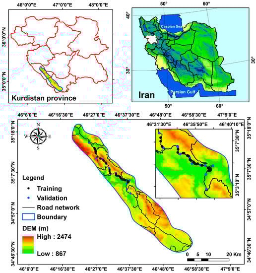
Figure 1.
The location of Kamyaran–Sarvabad road in Iran and Kurdistan province.
3. Landslide Conditioning Factors
A crucial next step for developing machine learning models is identifying the conditioning factors that can affect or cause the occurrence of landslides after gathering the dataset for landslides [27,28]. According to the presumption that new landslides are likely to occur in places with characteristics similar to those observed in the locations of prior landslides, a number of influential factors and a map of existing landslides need to be constructed before building the LSM [29].
We determined the following influencing factors and obtained the relative spatial layers using a literature review and analysis of previous landslide locations: slope, aspect, elevation, distance to river, river density, distance to road, distance to fault, road density, fault density, curvature, land use, lithology, SPI, and TWI (Figure 2) (Table 1). First, a 12.5 × 12.5 m digital elevation model (DEM) was produced using data from the ALOS PALSAR satellite from the Alaska satellite facility website (https://vertex.daac.asf.alaska.edu).
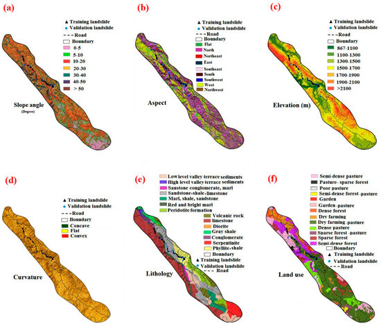
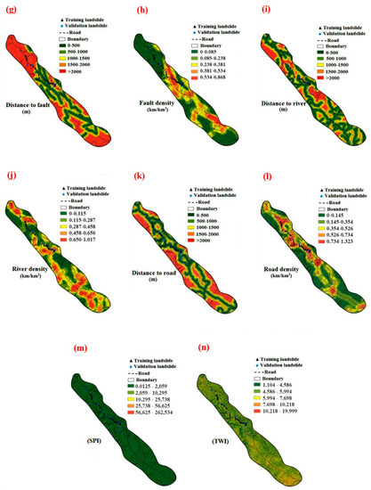
Figure 2.
Landslide influential factors utilized in the current study: (a) Slope, (b) Aspect, (c) Elevation, (d) Curvature, (e) Lithology, (f) Land use, (g) Distance to Fault, (h) Fault density, (i) Distance to river, (j) River density, (k) Distance to road, (l) Road density, (m) SPI, and (n) TWI.

Table 1.
Details of applied conditioning factors in the current study area.
Through the use of ArcGIS, we created slope, aspect, elevation, and curvature maps using the DEM. The seven classes, 0°–5°, 5°–10°, 10°–20°, 20°–30°, 30°–40°, 40°–50°, and >50° were used to categorise slopes (Figure 2a). Aspect was classified into nine classes, N, NE, E, SE, S, SW, W, NW, and Flat (Figure 2b). The DEM was used to derive an elevation map, which was then divided into seven classes, ranging from 867–1100, 1100–1300, 1300–1500, 1500–1700, 1700–1900, 1900–2100, and >2100 (Figure 2c). The slope was described as either having a convex or concave surface shape. In general, the curvature of the earth fluctuates between convex (positive), concave (negative), and flat (zero) values [30]. We mapped curvature in three classes of concave, convex, and flat (Figure 2d). A major controlling variable for the incidence of landslides is lithology [31], the lithology information derived at a scale of 1:100,000 from a geological map (Figure 2e). Since land use has an impact on hydrological conditions and soil strength, it is also regarded as a crucial landslide-controlling factor [32]. In this study, we categorized land use into 13 classes (Figure 2f). We obtained the faults map at a scale of 1:100,000 from the geological map and then computed the distance to faults using “Euclidean distance” tool in the ArcGIS 10.5 software. This was then classified into 5 classes including 0–500, 500–1000, 1000–1500, 1500–2000, and >2000 m (Figure 2g). We constructed a fault density map in five categorised including 0–0.085, 0.085–0.238, 0.238–0.381, 0.381–0.534, and 0.534–0.868 (km/km2) using the “Line density” tool in the ArcGIS 10.5 software (Figure 2h). Additionally, the “Euclidean distance” tool was used to map the distances to rivers, which were then divided into 5 categories: 0–500, 500–1000, 1000–1500, 1500–2000, and >2000 m (Figure 2i). The river density map was extracted using the “Line density” and then categorized into five classes including 0–0.115, 0.115–0.287, 0.287–0.458, 0.458–0.650, and 0.650–1.017 (km/km2) (Figure 2j).
Landslide susceptibility is known to decrease with increasing distance from main roads [33]. Thus, distance to roads was mapped by “Euclidean distance” tool and then categorised into 5 classes including 0–500, 500–1000, 1000–1500, 1500–2000, and >2000 m (Figure 2k). Road density is another factor that influences the incidence of landslides. It was extracted using the “Line density” and then categorized into five classes including 0–0.145, 0.145–0.354, 0.354–0.526, 0.526–0.734, and 0.734–1.323 (km/km2) (Figure 2l).
SPI was utilised to estimate how the topography affected hydrological processes [34]. The value of this parameter is computed from the following equation [35].
where AS () is the precise catchment area and β is the slope angle in degrees. Five categories were used to categorise the SPI map, including 0.0125–2059, 2059–10,295, 10,295–25,738, 25,738–56,625, and 56,625–262,534 (Figure 2m). TWI is important conditioning factor in the incidence of landslides [36]. This index is an index of elevation that captures the ratio between slopes in the basin. It is a measure of the geographical spread of soil wetness throughout the surface of the earth, and it may be calculated using the equation below [37].
where AS () denotes the precise catchment area, tgβ denotes the slope angle at that location, and α denotes the total upslope drainage via a point. Five classes were used to generate the TWI map in this investigation including 1.104–4.586, 4.586–5.994, 5.994–7.698, 7.698–10.218, and 10.218–19.999 (Figure 2n).
4. Methodology
The studied road is a mountainous road with a steep slope, and due to the fact that the areas of landslides were not recorded as polygons by organizations, we had to consider the landslide’s locations at the toe slope as the area prone to landslides (point locations by handy GPS) as they are clearly visible in the photos in Figure 3. The locations of 64 landslide points were identified by field surveys and checked on aerial photographs and Google Earth imageries.
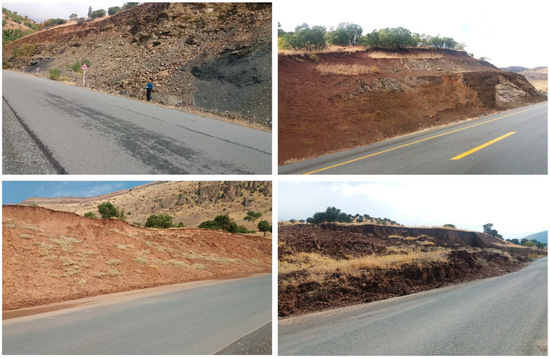
Figure 3.
Examples of landslides located along the Kamyaran–Sarvabad main road, Iran.
The field survey also indicated that most of the landslides are rotational slides. In total, 45 of these points were utilised for the training data, while 19 of these points were employed in the validation dataset. Then, using the training data and all conditioning parameters, three standard MLAs—RF, DT, and SVM—were used to identify the landslide-prone locations. The landslide point validation dataset was then used to validate the models (Figure 4).
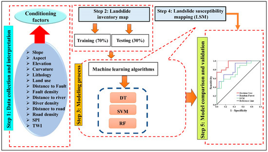
Figure 4.
The study’s proposed methodology’s schematic flowchart.
4.1. Landslide Inventory Map (LIM)
An inventory map for landslides is required for landslide modelling. After that, GIS-based statistical analysis can be used to determine the spatial association among landslides and landslide conditioning factors [38]. Landslides in a particular area are noted in the LIMs along with their position, action level, classification, and date. The primary cause of errors in LSM is a deficiency in the landslide inventory [39,40]. As mentioned above, we identified 64 landslide locations and used them either for model building and training (70%) and the rest for validation (30%). Figure 3 shows some images of landslides that have occurred in the research area.
4.2. Background of the MLAs
4.2.1. Random Forest
Using various selection methods to filter for specific features, we employed the critical features in the Random Forest (RF) model to determine their correlation with the classification. RFs are inherently random; therefore, the model may periodically assign different relevance weights to features [41,42]. By choosing the intersection of the final feature and a predetermined number of features, the model was trained. That way, a predetermined number of features is selected that significantly affects the classification process after repeatedly looping through this stage. The following is a more detailed explanation of how the significance of a particular feature X in RF is determined:
- (1)
- Determine each decision tree’s OOB error, denoted as errOOB1, using the matching out-of-bag (OOB) data in RF, with errOOB1 representing the average error for each calculation using only those predictions from the trees that are not contained in their respective bootstrap sample.
- (2)
- Add noise interference at random to every OOB sample, sampling feature X values. Additionally, a random adjustment may be made to the sample value at feature X. Recalculate the OOB data error after that, and then log the outcome as errOOB2.
- (3)
- Considering that RF contains NS trees, the following is the significance of feature X:
In this research, training was undertaken with 70% of the landslide data, and validation was performed with the remaining 30%. Two factors of decreasing mean accuracy and a Gini mean decreasing factor are used to rank each of the effective parameters in order of importance. The weights acquired for the effective factors in the R software 5.4 were then transferred to the ArcGIS environment, where they were used to create the final landslide map with five classes.
4.2.2. Support Vector Machines
Vapnik introduced the Support Vector Machine (SVM) for the first time (1995). Since then, many researchers have used it to examine natural and environmental hazards [43]. Its theoretical underpinnings are statistical learning theory. SVM is a machine learning classifier that has been employed to address a variety of problems in the real world, including landslide prediction [29,30,31,32,33,34,35,36,37,38,39,40,41,42,43,44].
The larger the separation plate is, the more stable the model will be against distortion and noise, and as a result, the greater its power will be for generalization. SVM model algorithms provide a holistic approach to estimating functions whose main focus is to solve quadratic optimization problems. Consider and corresponding to the factors affecting classified variables and the corresponding vectors of the two types of categorised variables (landslide and non-landslide). The ideal separation hyper plane can be defined as follows if and :
where , and are the offset from the original, n is the number of influencing elements for landslides, and the kernel functions might be polynomial, radial basis functions, sigmoid, or linear, accordingly [45].
4.2.3. Decision Tree Algorithm
A non-parametric method with a hierarchy of trees is called a decision tree (DT) model and can be used to uncover non-additive and non-linear correlations between targeting or predictive factors and input factors [46,47]. Classification trees and regression trees are the two main DT types. Regression trees are used for continuous data, while classification trees are used to predict discrete variables [48]. The primary benefit of the DT is that there is no need to transform variables because the structure of the model will remain the same without conversion; so, it saves time. It is also simple to design and analyse, and it may model complex interactions between variables.
DT modelling is often undertaken in two steps: 1—Tree construction; and 2—Tree pruning [38]. In many instances, pruning may be needed to prevent improper knots in the tree. A good algorithm is the algorithm that creates the largest tree and prunes it after measuring the ideal pruning threshold. There are two types of pruning: pre-pruning and post-pruning. When a tree is pre-pruned, it grows until a specific requirement is reached; however, when a tree is post-pruned, the entire tree is constructed. The interest rate for each node is calculated as per Equation (5):
where T is an educational data set that contains subset Ti (1, 2… n), and the profit ratio for the X characteristic is calculated as per the following Equations (6)–(8):
wherein
For the DT algorithm, Weak 3.9 software was used to run the modelling procedures.
4.2.4. Validation of the Models
Relative operator characteristics (ROC) were used to verify the three models. The x and y axes of the ROC curve, which correspond to the True Positive Rate (TPR) and False Positive Rate (FPR), capture the percentage of times that the true value is accurately predicted and the percentage of times that the false value is predicted to be true [49]. The training data and the susceptibility of landslides were compared to produce this curve.
The “area under this curve” is how the AUC is referred to. Furthermore, the model well with highest AUC will function much better [50]. AUC of 0.5 is the equivalent for the neutral model. The more closely the AUC value approaches one, the better the model performs [51].
4.2.5. Importance of the Factors Using Accuracy and the Gini Indexes
The results of the RF algorithm are examined in the form of two indicators including the accuracy index and the Gini index. By examining both of these indicators, the Gini factor was introduced as the most important input variable to the model. The Gini Index algorithm is based on the Gini theory. Let us assume S as a sample with k class (, and then we can classify S into k subsets by the differences between the classes. Consider as a sample set that belongs to a class , and therefore, the Gini index of the sample set is computed as follows:
where and are the probabilities of landslide occurrence in class and , respectively, which are computed with and , for each sample set of that belongs to [52,53].
5. Results
5.1. Importance of the Factors on Landslide Occurrence
The most significant factors and accompanying assessment indices affecting landslide susceptibility are shown in Table 2. Accordingly, the RF model revealed that slope and curvature parameters had the least influence on the probability of landslides. The model’s outcomes demonstrate that the model chose the distance to road, distance to river, road density, and TWI variables. Consequently, based on these factors, the decision tree is formed, which is most influenced by the distance to the road.
Table 2.
MDA and MDG indices based on a random forest model to determine conditioning factors of landslide susceptibility along the Kamyaran–Sarvabad main road.
5.2. Performance of the Random Forest Model
The error rate changes as the quantity of trees changes, as seen in Figure 5a. The error rate must be modified as the number of trees increases in order to determine the appropriate tree density. The RF algorithm’s estimates of the number of landslide and non-landslide spots are shown in this figure by classes 0 and 1, respectively. The OOB index also represents the estimates of the samples outside of the basket to observe how the error of the RT algorithm changes with increasing the number of trees. Based on the results shown in Figure 5a, all three errors have a similar decreasing trend as the number of trees increases. For the class 0, after alternating the increase and decrease using about 100 trees, the decreasing and increasing trend was repeated again until a constant trend was reached with about 380 trees. For class one, after alternating the increase and decrease using about 100 trees, a constant trend was found after repeating the decreasing and incremental trend in small intervals from about 280 trees onwards. For the OOB error, the increasing and decreasing trend was repeated and the error rate trend was fixed using about 380 trees. Figure 5b shows the ROC curve of the random forest algorithm. In this curve, the positive rate of accuracy versus the positive rate of error is displayed. As can be seen, the area below the curve is 0.96, which indicates a very high accuracy for this model.
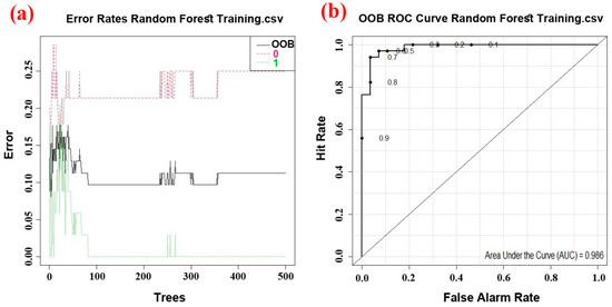
Figure 5.
Performance of the random forest model: (a) Error rate changes with an increasing number of trees (0 non-landslide, 1 landslide), (b) ROC curve based on out-of-basket estimates.
The modelling outcomes of this model demonstrated that the model chose four variables from the analysed variables, including distance to road, distance to river, road density, and TWI. The decision tree is created based on these variables, with distance to the road ranking highest.
5.3. Developing Landslide Susceptibility Maps
The final LSM was obtained by computing the weight of the layers for different conditioning factors in the occurrence of landslides and by obtaining the rate for each class along with the algebraic sum of the raster layers with the weight obtained for each layer of the data mining algorithms. Landslide susceptibly maps based on either an RF, DT, or SVM model are presented in Figure 6. Additionally, the area and the percentage of different classes of landslide potential in each of the three maps are presented in Table 3.
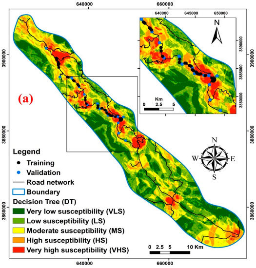
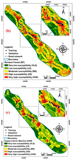
Figure 6.
Landslide susceptibility maps for the Kamyaran–Sarvabad main road, Iran, using three types of models: (a) Decision Tree (b) Random Forest, and (c) Support Vector Machine.
Table 3.
Area and percentage of landslides for each of the susceptibility classes identified for the Kamyaran–Sarvabad main road, Iran, using Support Vector Machine (SVM), Decision Tree (DT), and Random Forest (RF) models.
The ROC curve was used to assess the models that were employed. The AUC values for each model using the validation dataset are displayed in Table 4 and Figure 7. Accordingly, it is the chi-square’s asymptotic significance, or p-value, which we recently ran in SPSS. The statistical significance of the link we just investigated is determined by this value. In all significance tests, a link between the two variables is considered to be statistically significant if p < 0.05.
Table 4.
Area under the curve (AUC) results for the models utilising the validation dataset for the ROC curve.
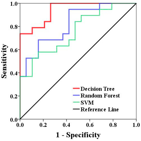
Figure 7.
ROC curve values for the models employed when utilising the validation dataset.
The “textbook” approach to creating confidence intervals is known as the asymptotic confidence interval (Asymptotic 95%). Despite the fact that it is valid for large sample sizes (thus the other moniker, “large-sample” confidence interval), there are no predetermined standards for how big is “large enough.” To put it another way, an exact confidence interval will result in the exact confidence level specified (for example, 95%); it is certain that if you repeated an experiment or poll repeatedly, you would obtain the same results 95% of the time [54]. The DT model demonstrated the greatest performance as compared to the SVM (AUC = 0.75), which demonstrated the lowest performance, with an AUC value of 0.94.
6. Discussion
The intensity and impact of natural hazards depends on their magnitude and severity. This information is critical, and tools are needed for hazard prediction to minimise human and financial loss [55]. Considering the body of research, the data’s accessibility, and the importance of the influencing variables for landslide incidence, as judged by the accuracy and Gini indices, resulting from the RF modelling, our study showed that the distance to the road, the road density, the distance to the river, the geology, and the land use were the five most important factors affecting landslide susceptibility. Constructing roads and not complying with the necessary standards and not protecting the cut-off areas creates dangerous conditions for the saturation of the underground layers, resulting in landslides—especially in places where the geological formation is susceptible and already eroded. Improper road construction and expansion in our study area are indeed the main factors for landslides to occur. The Kamyaran–Sarvabad main road’s high to extremely high landslide susceptibility zones in Iran’s Kurdistan province are located on the phyllite and slate and on the limestone and volcanic rocks covered by a soil layer. Similar results were reported by several others who also concluded that the most crucial factors for landslides to occur are the distance to the road and the density of the roads [56,57,58,59].
Furthermore, the current research showed that MLA models can assist decision-makers in identifying areas that are prone to landslides and may either be excluded from road and other development projects or managed in a way to make construction and use safe. The LSMs developed by all MLAs perform a great deal better than those made by [60]. In contrast to our analysis’s AUC ranges of 94% for DT and 0.82% for RF, their study’s AUC values ranged from 62.4% for GLM to 0.75% for RFs. Additionally, ref. [61], who used RFs for mapping landslide susceptibility along the Wadi Tayyah Basin in the Asir Region of Saudi Arabia, reported that our results for the RF with a prediction rate (AUC = 0.82%) were better.
Our results show that DT, RF, and SVM have respective prediction rates of 0.94, 0.82, and 0.75. We hypothesise that these disparities in prediction rates are due to the unique characteristics of each research location. The current study found potential contributing factors to landslides, and the findings and techniques can be used to create landslide inventory maps in other areas beyond our study area.
7. Conclusions
To produce landslide susceptibility maps for the main road between Kamyaran and Sarvabad, we evaluated SVM, DT, and RF models. The following results in this study can be highlighted:
- (1)
- According to the results for two indices, Mean Decrease Accuracy and Mean Decrease Gini, the RF model was the most accurate in identifying the significance of landslide conditioning factors that caused landslide events in the current experiment. The most important factors in landslide susceptibility modelling for our research region include the distance to roads, road density, distance to rivers, geology, land use, elevation, distance to faults, aspect, fault density SPI, slope, TWI, and curvature.
- (2)
- LSMs were prepared using RF, DT, and SVM models adopting parameter tuning techniques. According on our research, the RF model performed and outperformed the DT and SVM models.
- (3)
- According to the landslide susceptibility maps, the most vulnerable locations are close to roads and follow the density of those roads. They are primarily in the middle of the research area as a result. The findings of this study can thus assist land developers, planners, and civil engineers with preliminary slope management and land-use planning, allowing them to take essential and scientific action to avert landslide dangers.
The best way to lessen the impact of landslides is to develop a map of landslide susceptibility at the national, regional, and local levels. This map can be used to identify risky regions and prevent damage before a disaster strikes. In the future, weight analysis that accounts for predisposing variables will be used to better study these factors. Furthermore, we believe that our prediction model will incorporate landslide risk management and LSM using more potent machine and deep learning architectures.
Author Contributions
Contributing equally to the work, H.S., R.A., M.A., M.H., N.A.-A., A.S., I.D.W. and E.H.A. collected field data and conducted the landslide susceptibility analysis; E.H.A. wrote the manuscript; M.H., N.A.-A., I.D.W. and E.H.A. provided critical comments in planning this paper and edited the manuscript. All the authors discussed the results and edited the manuscript. All authors have read and agreed to the published version of the manuscript.
Funding
This research was funded by the University of Kurdistan, Iran, based on two grants numbered 02-9-3786 and 01-9-22595 (Himan Shahabi and Ataollah Shirzadi) of highly cited researchers in the top 1% of the world (according to the ISC list).
Acknowledgments
The authors thank the University of Kurdistan, Iran, and Universiti Teknologi Malaysia (UTM) for preparing this international collaboration for the scientific sharing experience.
Conflicts of Interest
The authors declare no conflict of interest.
References
- Assilzadeh, H.; Levy, J.K.; Wang, X. Landslide catastrophes and disaster risk reduction: A GIS framework for landslide prevention and management. Remote Sens. 2010, 2, 2259–2273. [Google Scholar] [CrossRef]
- Gordo, C.; Zêzere, J.L.; Marques, R. Landslide susceptibility assessment at the basin scale for rainfall-and earthquake-triggered shallow slides. Geosciences 2019, 9, 268. [Google Scholar] [CrossRef]
- Jones, S.; Kasthurba, A.; Bhagyanathan, A.; Binoy, B. Impact of anthropogenic activities on landslide occurrences in southwest India: An investigation using spatial models. J. Earth Syst. Sci. 2021, 130, 70. [Google Scholar] [CrossRef]
- Tehrani, F.S.; Calvello, M.; Liu, Z.; Zhang, L.; Lacasse, S. Machine learning and landslide studies: Recent advances and applications. Nat. Hazards 2022, 114, 1197–1245. [Google Scholar] [CrossRef]
- Saha, S.; Sarkar, R.; Roy, J.; Hembram, T.K.; Acharya, S.; Thapa, G.; Drukpa, D. Measuring landslide vulnerability status of Chukha, Bhutan using deep learning algorithms. Sci. Rep. 2021, 11, 16374. [Google Scholar] [CrossRef]
- Mavroulis, S.; Diakakis, M.; Kranis, H.; Vassilakis, E.; Kapetanidis, V.; Spingos, I.; Kaviris, G.; Skourtsos, E.; Voulgaris, N.; Lekkas, E. Inventory of Historical and Recent Earthquake-Triggered Landslides and Assessment of Related Susceptibility by GIS-Based Analytic Hierarchy Process: The Case of Cephalonia (Ionian Islands, Western Greece). Appl. Sci. 2022, 12, 2895. [Google Scholar] [CrossRef]
- Petrova, E. Natural hazard impacts on transport infrastructure in Russia. Nat. Hazards Earth Syst. Sci. 2020, 20, 1969–1983. [Google Scholar] [CrossRef]
- Khaliq, A.H.; Basharat, M.; Riaz, M.T.; Riaz, M.T.; Wani, S.; Al-Ansari, N.; Le, L.B.; Linh, N.T.T. Spatiotemporal landslide susceptibility mapping using machine learning models: A case study from district Hattian Bala, NW Himalaya, Pakistan. Ain Shams Eng. J. 2022, 101907. [Google Scholar]
- Aghdam, I.N.; Pradhan, B.; Panahi, M. Landslide susceptibility assessment using a novel hybrid model of statistical bivariate methods (FR and WOE) and adaptive neuro-fuzzy inference system (ANFIS) at southern Zagros Mountains in Iran. Environ. Earth Sci. 2017, 76, 237. [Google Scholar] [CrossRef]
- Ghasemian, B.; Shahabi, H.; Shirzadi, A.; Al-Ansari, N.; Jaafari, A.; Geertsema, M.; Melesse, A.M.; Singh, S.K.; Ahmad, A. Application of a Novel Hybrid Machine Learning Algorithm in Shallow Landslide Susceptibility Mapping in a Mountainous Area. Front. Environ. Sci. 2022, 10, 657. [Google Scholar] [CrossRef]
- Bai, S.-B.; Wang, J.; Lü, G.-N.; Zhou, P.-G.; Hou, S.-S.; Xu, S.-N. GIS-based logistic regression for landslide susceptibility mapping of the Zhongxian segment in the Three Gorges area, China. Geomorphology 2010, 115, 23–31. [Google Scholar] [CrossRef]
- Akinci, H.; Yavuz Ozalp, A. Landslide susceptibility mapping and hazard assessment in Artvin (Turkey) using frequency ratio and modified information value model. Acta Geophys. 2021, 69, 725–745. [Google Scholar] [CrossRef]
- Huang, J.; Zhou, Q.; Wang, F. Mapping the landslide susceptibility in Lantau Island, Hong Kong, by frequency ratio and logistic regression model. Ann. GIS 2015, 21, 191–208. [Google Scholar] [CrossRef]
- Erener, A.; Mutlu, A.; Düzgün, H.S. A comparative study for landslide susceptibility mapping using GIS-based multi-criteria decision analysis (MCDA), logistic regression (LR) and association rule mining (ARM). Eng. Geol. 2016, 203, 45–55. [Google Scholar] [CrossRef]
- Dikshit, A.; Pradhan, B.; Alamri, A.M. Pathways and challenges of the application of artificial intelligence to geohazards modelling. Gondwana Res. 2021, 100, 290–301. [Google Scholar] [CrossRef]
- Wang, X.; Huang, F.; Fan, X.; Shahabi, H.; Shirzadi, A.; Bian, H.; Ma, X.; Lei, X.; Chen, W. Landslide susceptibility modeling based on remote sensing data and data mining techniques. Environ. Earth Sci. 2022, 81, 50. [Google Scholar] [CrossRef]
- Akinci, H.; Zeybek, M. Comparing classical statistic and machine learning models in landslide susceptibility mapping in Ardanuc (Artvin), Turkey. Nat. Hazards 2021, 108, 1515–1543. [Google Scholar] [CrossRef]
- Chen, W.; Panahi, M.; Tsangaratos, P.; Shahabi, H.; Ilia, I.; Panahi, S.; Li, S.; Jaafari, A.; Ahmad, B.B. Applying population-based evolutionary algorithms and a neuro-fuzzy system for modeling landslide susceptibility. Catena 2019, 172, 212–231. [Google Scholar] [CrossRef]
- Tsangaratos, P.; Ilia, I. Landslide susceptibility mapping using a modified decision tree classifier in the Xanthi Perfection, Greece. Landslides 2016, 13, 305–320. [Google Scholar] [CrossRef]
- Tien Bui, D.; Tuan, T.A.; Klempe, H.; Pradhan, B.; Revhaug, I. Spatial prediction models for shallow landslide hazards: A comparative assessment of the efficacy of support vector machines, artificial neural networks, kernel logistic regression, and logistic model tree. Landslides 2016, 13, 361–378. [Google Scholar] [CrossRef]
- Sevgen, E.; Kocaman, S.; Nefeslioglu, H.A.; Gokceoglu, C. A novel performance assessment approach using photogrammetric techniques for landslide susceptibility mapping with logistic regression, ANN and random forest. Sensors 2019, 19, 3940. [Google Scholar] [CrossRef]
- Akinci, H. Assessment of rainfall-induced landslide susceptibility in Artvin, Turkey using machine learning techniques. J. Afr. Earth Sci. 2022, 191, 104535. [Google Scholar] [CrossRef]
- Zhang, W.; Li, H.; Han, L.; Chen, L.; Wang, L. Slope stability prediction using ensemble learning techniques: A case study in Yunyang County, Chongqing, China. J. Rock Mech. Geotech. Eng. 2022, 14, 1089–1099. [Google Scholar] [CrossRef]
- Piacentini, D.; Devoto, S.; Mantovani, M.; Pasuto, A.; Prampolini, M.; Soldati, M. Landslide susceptibility modeling assisted by Persistent Scatterers Interferometry (PSI): An example from the northwestern coast of Malta. Nat. Hazards 2015, 78, 681–697. [Google Scholar] [CrossRef]
- Ghorbanzadeh, O.; Xu, Y.; Zhao, H.; Wang, J.; Zhong, Y.; Zhao, D.; Zang, Q.; Wang, S.; Zhang, F.; Shi, Y. The Outcome of the 2022 Landslide4Sense Competition: Advanced Landslide Detection From Multisource Satellite Imagery. IEEE J. Sel. Top. Appl. Earth Obs. Remote Sens. 2022, 15, 9927–9942. [Google Scholar] [CrossRef]
- Ghorbanzadeh, O.; Gholamnia, K.; Ghamisi, P. The application of ResU-net and OBIA for landslide detection from multi-temporal sentinel-2 images. Big Earth Data 2022, 1–26. [Google Scholar] [CrossRef]
- He, Q.; Shahabi, H.; Shirzadi, A.; Li, S.; Chen, W.; Wang, N.; Chai, H.; Bian, H.; Ma, J.; Chen, Y. Landslide spatial modelling using novel bivariate statistical based Naïve Bayes, RBF Classifier, and RBF Network machine learning algorithms. Sci. Total Environ. 2019, 663, 1–15. [Google Scholar] [CrossRef]
- Ghorbanzadeh, O.; Blaschke, T.; Gholamnia, K.; Meena, S.R.; Tiede, D.; Aryal, J. Evaluation of different machine learning methods and deep-learning convolutional neural networks for landslide detection. Remote Sens. 2019, 11, 196. [Google Scholar] [CrossRef]
- Huang, Y.; Zhao, L. Review on landslide susceptibility mapping using support vector machines. Catena 2018, 165, 520–529. [Google Scholar] [CrossRef]
- Pourghasemi, H.R.; Pradhan, B.; Gokceoglu, C. Application of fuzzy logic and analytical hierarchy process (AHP) to landslide susceptibility mapping at Haraz watershed, Iran. Nat. Hazards 2012, 63, 965–996. [Google Scholar] [CrossRef]
- Lan, H.; Zhou, C.; Wang, L.; Zhang, H.; Li, R. Landslide hazard spatial analysis and prediction using GIS in the Xiaojiang watershed, Yunnan, China. Eng. Geol. 2004, 76, 109–128. [Google Scholar] [CrossRef]
- Kornejady, A.; Ownegh, M.; Bahremand, A. Landslide susceptibility assessment using maximum entropy model with two different data sampling methods. Catena 2017, 152, 144–162. [Google Scholar] [CrossRef]
- Yilmaz, I. Comparison of landslide susceptibility mapping methodologies for Koyulhisar, Turkey: Conditional probability, logistic regression, artificial neural networks, and support vector machine. Environ. Earth Sci. 2010, 61, 821–836. [Google Scholar] [CrossRef]
- Crosby, D.A. The Effect of DEM Resolution on the Computation of Hydrologically Significant Topographic Attributes. Master’s Thesis, University of South Florida, Tampa, FL, USA, 2006. [Google Scholar]
- Devkota, K.C.; Regmi, A.D.; Pourghasemi, H.R.; Yoshida, K.; Pradhan, B.; Ryu, I.C.; Dhital, M.R.; Althuwaynee, O.F. Landslide susceptibility mapping using certainty factor, index of entropy and logistic regression models in GIS and their comparison at Mugling–Narayanghat road section in Nepal Himalaya. Nat. Hazards 2013, 65, 135–165. [Google Scholar] [CrossRef]
- Lee, S.; Lee, M.-J.; Lee, S. Spatial prediction of urban landslide susceptibility based on topographic factors using boosted trees. Environ. Earth Sci. 2018, 77, 656. [Google Scholar] [CrossRef]
- Sezer, E.A.; Nefeslioglu, H.A.; Osna, T. An expert-based landslide susceptibility mapping (LSM) module developed for Netcad Architect Software. Comput. Geosci. 2017, 98, 26–37. [Google Scholar] [CrossRef]
- Tien Bui, D.; Pradhan, B.; Lofman, O.; Revhaug, I. Landslide susceptibility assessment in vietnam using support vector machines, decision tree, and Naive Bayes Models. Math. Probl. Eng. 2012, 2012, 974638. [Google Scholar] [CrossRef]
- Van Westen, C.J.; Castellanos, E.; Kuriakose, S.L. Spatial data for landslide susceptibility, hazard, and vulnerability assessment: An overview. Eng. Geol. 2008, 102, 112–131. [Google Scholar] [CrossRef]
- Pellicani, R.; Spilotro, G. Evaluating the quality of landslide inventory maps: Comparison between archive and surveyed inventories for the Daunia region (Apulia, Southern Italy). Bull. Eng. Geol. Environ. 2015, 74, 357–367. [Google Scholar] [CrossRef]
- De Oliveira, G.G.; Ruiz, L.F.C.; Guasselli, L.A.; Haetinger, C. Random forest and artificial neural networks in landslide susceptibility modeling: A case study of the Fão River Basin, Southern Brazil. Nat. Hazards 2019, 99, 1049–1073. [Google Scholar] [CrossRef]
- Trigila, A.; Iadanza, C.; Esposito, C.; Scarascia-Mugnozza, G. Comparison of Logistic Regression and Random Forests techniques for shallow landslide susceptibility assessment in Giampilieri (NE Sicily, Italy). Geomorphology 2015, 249, 119–136. [Google Scholar] [CrossRef]
- Vapnik, V. The Nature of Statistical Learning Theory; Springer Science & Business Media: Berlin/Heidelberg, Germany, 1999. [Google Scholar]
- Hong, H.; Pradhan, B.; Bui, D.T.; Xu, C.; Youssef, A.M.; Chen, W. Comparison of four kernel functions used in support vector machines for landslide susceptibility mapping: A case study at Suichuan area (China). Geomat. Nat. Hazards Risk 2017, 8, 544–569. [Google Scholar] [CrossRef]
- Dixon, B.; Candade, N. Multispectral landuse classification using neural networks and support vector machines: One or the other, or both? Int. J. Remote Sens. 2008, 29, 1185–1206. [Google Scholar] [CrossRef]
- Fielding, A. Machine Learning Methods for Ecological Applications; Springer Science & Business Media: Berlin/Heidelberg, Germany, 1999. [Google Scholar]
- Jones, M.J.; Fielding, A.; Sullivan, M. Analysing extinction risk in parrots using decision trees. Biodivers. Conserv. 2006, 15, 1993–2007. [Google Scholar] [CrossRef]
- Nefeslioglu, H.; Sezer, E.; Gokceoglu, C.; Bozkir, A.; Duman, T. Assessment of landslide susceptibility by decision trees in the metropolitan area of Istanbul, Turkey. Math. Probl. Eng. 2010, 2010, 901095. [Google Scholar] [CrossRef]
- Uwihirwe, J.; Hrachowitz, M.; Bogaard, T.A. Landslide precipitation thresholds in Rwanda. Landslides 2020, 17, 2469–2481. [Google Scholar] [CrossRef]
- Youssef, A.M.; Pourghasemi, H.R. Landslide susceptibility mapping using machine learning algorithms and comparison of their performance at Abha Basin, Asir Region, Saudi Arabia. Geosci. Front. 2021, 12, 639–655. [Google Scholar] [CrossRef]
- Lee, D.-H.; Kim, Y.-T.; Lee, S.-R. Shallow landslide susceptibility models based on artificial neural networks considering the factor selection method and various non-linear activation functions. Remote Sens. 2020, 12, 1194. [Google Scholar] [CrossRef]
- Algehyne, E.A.; Jibril, M.L.; Algehainy, N.A.; Alamri, O.A.; Alzahrani, A.K. Fuzzy neural network expert system with an improved Gini index random forest-based feature importance measure algorithm for early diagnosis of breast cancer in Saudi Arabia. Big Data Cogn. Comput. 2022, 6, 13. [Google Scholar] [CrossRef]
- Park, S.; Hamm, S.-Y.; Kim, J. Performance evaluation of the GIS-based data-mining techniques decision tree, random forest, and rotation forest for landslide susceptibility modeling. Sustainability 2019, 11, 5659. [Google Scholar] [CrossRef]
- Geyer, C.J. Stat 5102 notes: More on confidence intervals. Univ. Minn. 2003, 24, 1–16. [Google Scholar]
- Tsakiris, G.; Pangalou, D.; Vangelis, H. Regional drought assessment based on the Reconnaissance Drought Index (RDI). Water Resour. Manag. 2007, 21, 821–833. [Google Scholar] [CrossRef]
- Postance, B.; Hillier, J.; Dijkstra, T.; Dixon, N. Extending natural hazard impacts: An assessment of landslide disruptions on a national road transportation network. Environ. Res. Lett. 2017, 12, 014010. [Google Scholar] [CrossRef]
- Jaafari, A.; Rezaeian, J.; Omrani, M.S.O. Spatial prediction of slope failures in support of forestry operations safety. Croat. J. For. Eng. J. Theory Appl. For. Eng. 2017, 38, 107–118. [Google Scholar]
- Schlögl, M.; Richter, G.; Avian, M.; Thaler, T.; Heiss, G.; Lenz, G.; Fuchs, S. On the nexus between landslide susceptibility and transport infrastructure–an agent-based approach. Nat. Hazards Earth Syst. Sci. 2019, 19, 201–219. [Google Scholar] [CrossRef]
- Pham, B.T.; Nguyen-Thoi, T.; Qi, C.; Van Phong, T.; Dou, J.; Ho, L.S.; Van Le, H.; Prakash, I. Coupling RBF neural network with ensemble learning techniques for landslide susceptibility mapping. Catena 2020, 195, 104805. [Google Scholar] [CrossRef]
- Pourghasemi, H.R.; Rahmati, O. Prediction of the landslide susceptibility: Which algorithm, which precision? Catena 2018, 162, 177–192. [Google Scholar] [CrossRef]
- Youssef, A.M.; Pourghasemi, H.R.; Pourtaghi, Z.S.; Al-Katheeri, M.M. Landslide susceptibility mapping using random forest, boosted regression tree, classification and regression tree, and general linear models and comparison of their performance at Wadi Tayyah Basin, Asir Region, Saudi Arabia. Landslides 2016, 13, 839–856. [Google Scholar] [CrossRef]
Disclaimer/Publisher’s Note: The statements, opinions and data contained in all publications are solely those of the individual author(s) and contributor(s) and not of MDPI and/or the editor(s). MDPI and/or the editor(s) disclaim responsibility for any injury to people or property resulting from any ideas, methods, instructions or products referred to in the content. |
© 2023 by the authors. Licensee MDPI, Basel, Switzerland. This article is an open access article distributed under the terms and conditions of the Creative Commons Attribution (CC BY) license (https://creativecommons.org/licenses/by/4.0/).