Article

Orthomosaicking Thermal Drone Images of Forests via Simultaneously Acquired RGB Images

by
Rudraksh Kapil
1,2,*,
Guillermo Castilla
3,
Seyed Mojtaba Marvasti-Zadeh
2,
Devin Goodsman
3,
Nadir Erbilgin
2,† and
Nilanjan Ray
1,†
1
Department of Computing Science, University of Alberta, 116 Street & 85 Avenue, Edmonton, AB T6G 2R3, Canada
2
Department of Renewable Resources, University of Alberta, 116 Street & 85 Avenue, Edmonton, AB T6G 2R3, Canada
3
Northern Forestry Centre, Canadian Forest Service, Natural Resources Canada, 5320 122 Street NW, Edmonton, AB T6H 3S5, Canada
*
Author to whom correspondence should be addressed.
These authors contributed equally to this work.
Remote Sens. 2023, 15(10), 2653; https://doi.org/10.3390/rs15102653
Submission received: 17 April 2023 / Revised: 16 May 2023 / Accepted: 17 May 2023 / Published: 19 May 2023
(This article belongs to the Collection Feature Paper Special Issue on Forest Remote Sensing)

Abstract

:
Operational forest monitoring often requires fine-detail information in the form of an orthomosaic, created by stitching overlapping nadir images captured by aerial platforms such as drones. RGB drone sensors are commonly used for low-cost, high-resolution imaging that is conducive to effective orthomosaicking, but only capture visible light. Thermal sensors, on the other hand, capture long-wave infrared radiation, which is useful for early pest detection among other applications. However, these lower-resolution images suffer from reduced contrast and lack of descriptive features for successful orthomosaicking, leading to gaps or swirling artifacts in the orthomosaic. To tackle this, we propose a thermal orthomosaicking workflow that leverages simultaneously acquired RGB images. The latter are used for producing a surface mesh via structure from motion, while thermal images are only used to texture this mesh and yield a thermal orthomosaic. Prior to texturing, RGB-thermal image pairs are co-registered using an affine transformation derived from a machine learning technique. On average, the individual RGB and thermal images achieve a mutual information of 0.2787 after co-registration using our technique, compared to 0.0591 before co-registration, and 0.1934 using manual co-registration. We show that the thermal orthomosaic generated from our workflow (1) is of better quality than other existing methods, (2) is geometrically aligned with the RGB orthomosaic, (3) preserves radiometric information (i.e., surface temperatures) from the original thermal imagery, and (4) enables easy transfer of downstream tasks—such as tree crown detection from the RGB to the thermal orthomosaic. We also provide an open-source tool that implements our workflow to facilitate usage and further development.

Graphical Abstract

1. Introduction

Forests are essential ecosystems that provide immense economic, social, and ecological value. Monitoring forest health is critical to understanding the challenges these ecosystems face and devising successful management strategies to foster healthy and resilient forests [1]. For example, forest monitoring is important for the detection of bark beetle attacks [2,3] and assessing tree losses due to deforestation [4]. In recent years, drones have become increasingly popular for close-range monitoring of forests to capture high-resolution images of focus areas [5,6,7,8]. Drones can be fitted with multiple-sensor instruments that take synchronized nadir images at regular intervals as the drone flies over areas to be imaged [9]. Optical sensors that capture information from various parts of the electromagnetic spectrum are commonly used for forest health monitoring applications [5]. Among them, RGB sensors take images in the visible range of the spectrum (i.e., three channels—red, green, and blue) and have been extensively used for many applications, owing to their low cost and high resolution [10]. On the other hand, thermal sensors capture images that measure surface temperatures, which is beneficial for numerous applications, e.g., forest fire monitoring [11] or detection of insect-induced canopy temperature increases [12], for instance, those created by bark beetle infestations of Norway spruce (Pinus abies) trees [13]. To facilitate monitoring in Geographic Information Systems (GIS) for such applications, drone-collected images need to be orthorectified and stitched together to generate an orthophoto mosaic (hereafter orthomosaic). For instance, a GIS polygon layer with the location, size, and shape of the crowns of young trees can be automatically derived by an artificial intelligence (AI) from a drone RGB orthomosaic of a regenerating cut block [14].
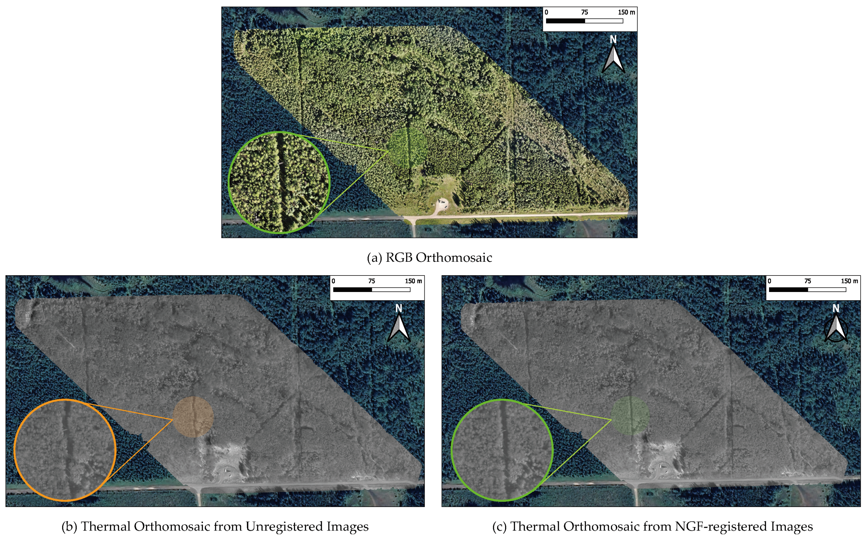
Existing workflows usually generate orthomosaics for RGB and thermal data of forests separately [15]. However, thermal images typically lack enough contrast and salient features to enable smooth orthomosaicking [16], and temperature fluctuations can create different salient features in overlapping images from adjacent flight lines [17]. Hence, some practitioners prefer to skip the thermal orthomosaic entirely and directly work with individual thermal images [12,18], but this complicates the transferral of information to GIS. Specifically, current standard methods that work well for RGB images [10] cannot reliably generate orthomosaics when it comes to thermal images of forests and crop fields [17,19,20,21]. Thermal orthomosaics generated with these standard workflows suffer from swirling artifacts as well as gaps, leading to incomplete coverage of the entire area of interest (Figure 1a). These artifacts are caused by poor depth estimation during the structure from motion (SfM) [22] stage of orthomosaicking [23].
Previous works have attempted to leverage simultaneously acquired RGB imagery to overcome the drawbacks of thermal-only workflows. A technique to improve the thermal orthomosaicking workflow by deriving the thermal image positions using RGB image alignment was proposed in [17]. Once the RGB image alignment is optimized, the external orientation parameters (xyz coordinates along with pitch, yaw, and roll angles) of each image are transferred to its thermal counterpart, and these are used as initial parameters in the SfM workflow for the set of thermal images. While a viable option, the second SfM process may introduce artifacts due to the previously mentioned issues inherent to thermal images. Likewise, [24] performed SfM for RGB and thermal images separately prior to registering (aligning) the resulting point clouds for the multi-modal 3D reconstruction of buildings. However, the thermal SfM step can introduce issues here as well. Similar to [17,25] proposed a workflow in which the external orientations of the RGB–thermal image pairs were aligned, but without any subsequent registration step. As the authors observed, using unregistered images leads to errors in the mosaic even for the urban setting they considered. Another combined approach was proposed in [26], where each pair of RGB and thermal images was stacked into a 4-channel image prior to orthomosaicking and separated afterward. However, this method requires an additional object-based geometric alignment stage that relies on the manual selection of objects clearly visible in both types of images and that cannot fully resolve distortions due to different focal lengths in the lenses of the thermal and RGB cameras. Similarly, [27] used a technique that relies on manually supplied pixel location correspondences between image pairs to fuse RGB and thermal point clouds of 3D structures. As precursors of our proposed automated co-registration (i.e., aligning the pixel-wise geometry of image pairs), the enhanced correlation coefficient (ECC) [28] was applied with varying levels of success to RGB and thermal images of crop fields at different heights: [29] used ECC to register images taken 1.6 m above the crop canopy, [30] applied ECC-based registration to drone imagery at a flight height of 30 m, and more recently, [31] used ECC to register images of olive groves at a 45–50 m altitude for generating aligned point clouds. However, these studies did not include the generation of orthomosaics. An edge feature-based image registration technique with the aid of image metadata was proposed in [32], whereas other works relied on point feature extraction [33,34,35]. Although these methods perform well for urban/generic settings, their application to nadir forest images is limited due to the lack of distinctive features in these scenarios. Moreover, they did not include orthomosaicking.
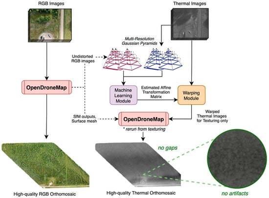
We propose a new integrated RGB and thermal processing workflow to overcome the mentioned challenges of thermal orthomosaicking of forest imagery. It is applicable to drone instruments that can simultaneously capture both RGB and thermal images. The proposed workflow is summarized in Figure 1b. It relies on an orthomosaicking algorithm based on texture mapping, as implemented in [36]. Texturing is a crucial step in this implementation of orthomosaicking, where rather than orthorectifying and stitching together the individual drone photos, a 2.5D mesh representing the outer envelope of the dense point cloud is created, and then the mesh is textured by projecting onto each small triangular mesh surface a particular patch of a drone photo from which it is best observed; the orthomosaic is then simply the orthographic projection of that textured mesh. Following this process applied directly to the RGB images, we obtain an orthomosaic along with important intermediate outputs—a surface mesh of the study site, the estimated external camera orientations used for texturing, and undistorted RGB images that have been corrected for radial and tangential distortions. Next, we co-register the simultaneously acquired RGB–thermal image pairs and rerun the orthomosaicking process from the texturing step using the intermediate RGB outputs. This involves re-texturing the previously constructed surface mesh with the thermal images, based on the camera orientations estimated using the RGB images. Thus, we generate two geometrically aligned orthomosaics, where the same objects appear in the same pixel locations of both the RGB and thermal orthomosaics. Because we do not use thermal images for SfM, which would perform poorly due to the low contrast and lack of features in these images, we avoid the gap and swirling issues present in thermal-only orthomosaicking workflows, as shown in Figure 1b.
Before the RGB intermediate outputs can be reused with the thermal images as described, we need to precisely align the geometry of the individual thermal and RGB images to ensure that objects appear in the same pixel locations in each RGB–thermal pair. We do this through an intensity-based image co-registration method using gradient descent, inspired by [37,38]. In particular, the precise co-registration of RGB–thermal pairs is achieved through a multi-scale framework utilizing the matrix exponential representation [39,40] and the normalized gradient fields (NGF) loss function [38]. According to [38] and confirmed by our results, this loss function is more suitable than ECC for multi-modal drone imagery of forests. The co-registered thermal images are what we use to replace the RGB undistorted images prior to rerunning the orthomosaicking process.
Rather than relying on manually selected objects like in [26,27], our geometric alignment is automated and offers more degrees of freedom than just displacement. In addition, bypassing the SfM process for the thermal images helps overcome the issues of lower contrast and lower resolution, and is thus preferable to previous feature-based techniques [32,33,34,35]. The proposed workflow assumes that the RGB and thermal nadir images are captured simultaneously during the same flight (i.e., using a multi-sensor setup), which is the case for many commercially available drone cameras, for instance, the DJI Zenmuse H20T, DJI Zenmuse XT2, DJI Mavic 3T, senseFly Duet T, FLIR Hadron RGB/Thermal Camera Module, and Autel EVO II Dual 640T. A slight delay in the capture times of the two sensors does not cause any problems, so long as the delay is systematic and there are an equal number of RGB and thermal images taken during the flight.
We demonstrate the effectiveness of our proposed orthomosaicking workflow using drone data from multiple dates over a forest stand in central Alberta, Canada. Aside from the high quality of the thermal orthomosaics generated (no gaps or swirling artifacts), we also demonstrate that the orthomosaicking process preserves the radiometry of the images—both the individual thermal images and the corresponding part of the generated orthomosaic have the same thermal information. To highlight the utility of our proposed workflow that outputs geometrically aligned RGB and thermal orthomosaics, we use a pre-trained deep learning model for individual tree crown detection from RGB images [41]. We show that the bounding boxes detected from the RGB orthomosaic can be directly used to extract tree crowns from the thermal orthomosaic (since they appear at the same pixel locations). As a further contribution, we provide a tool with an extensive graphical user interface (GUI) that simplifies the implementation of our integrated RGB–thermal orthomosaic generation workflow. The developed tool is open-source to facilitate modification for specific projects and to encourage the integration of additional functionalities.
In summary, the contributions presented in this paper are the following:
  • We propose an integrated RGB and thermal orthomosaic generation workflow that bypasses the need for thermal SfM by leveraging intermediate RGB orthomosaicking outputs and co-registering RGB and thermal images through an automated intensity-based technique.
  • We show that our workflow overcomes common issues associated with thermal-only orthomosaicking workflows while preserving the radiometric information (absolute temperature values) in the thermal imagery.
  • We demonstrate the effectiveness of the geometrically aligned orthomosaics generated from our proposed workflow by utilizing an existing deep learning-based tree crown detector, showing how the RGB-detected bounding boxes can be directly applied to the thermal orthomosaic to extract thermal tree crowns.
  • We develop an open-source tool with a GUI that implements our workflow to aid practitioners.

2. Materials and Proposed Workflow

We first describe the dataset used in our experiments and then provide an in-depth description of the proposed integrated orthomosaicking workflow for thermal images. Following this, we explain how an example downstream task is used to highlight the utility of our workflow. Next, we outline our GUI tool that implements the proposed workflow, as well as provide recommendations for its use. At the end, we describe how we empirically assessed the performance of our proposed method.

2.1. Cynthia Cutblock Study Site

We repeatedly collected drone data from an 8-hectare forest stand approximately 3.5 km to the northeast of Cynthia, central Alberta (Canada), referred to as the Cynthia cutblock in this paper. The location is shown in Figure 2. The region is at an elevation of around 950 m above sea level. Lodgepole pine (Pinus contorta ssp. latifolia) and aspen (Populus tremuloides) make up the majority of the tree species found within the cutblock. A Zenmuse H20T instrument mounted on a DJI Matrice 300 RTK quadcopter was used to take nadir RGB and thermal images of the cutblock. The H20T is fitted with three cameras. The wide-angle RGB camera takes images of 3040 × 4056 pixels and covers the most terrain ( 83 ° field of view (FOV)). The thermal images are 650 × 512 pixels and have a FOV of 41 ° . The zoom camera (not used in this study) can go up to 4 ° FOV and has dimensions of 5184 × 3888 pixels. The two RGB sensors are CMOS sensors, whereas the thermal one is an uncooled VOx microbolometer that produces 16-bit radiometric JPEGs (RJPEGs). We considered a total of five flights on different days in 2022 over the Cynthia cutblock using the described camera setup (20 July, 26 July, 9 August, 17 August, and 30 August). Each flight lasted approximately 30 min and was conducted between 10 a.m. and 1 p.m. Weather conditions varied across all flights—air temperature was between 20 °C and 25 °C, relative humidity was between 40% and 61%, and cloud cover was limited. Specific air temperature and relative humidity values during each flight are reported in Table 1, where the values are averages from the three nearest weather stations. The drone was flown at 120 m above the ground, following the same flight path across all dates. The thermal and wide-angle RGB images were taken simultaneously, such that thermal images had a 75% side overlap and 80% front overlap. Roughly the same number of image pairs (∼800) were captured during all flights. The EXIF header of each JPEG image contains the GPS coordinates of the drone when that image was taken. This information is helpful for individual image localization and georeferencing during the orthomosaicking process. Each output orthomosaic covers an area of around 30 hectares encompassing the cutblock.

2.2. Proposed Integrated Orthomosaicking Workflow

Here, we describe our proposed workflow for generating a thermal orthomosaic by leveraging RGB data. Our workflow relies on Open Drone Map (ODM) [36], an open-source framework that implements a texturing-based orthomosaicking algorithm similar to that described in [42]. ODM is described in further detail in Section 2.2.1, but briefly, a textured surface mesh reconstruction of the scene is first produced to yield an orthomosaic, rather than relying on a digital surface model (DSM) for orthorectification of images prior to stitching. We leverage the intermediate outputs generated from the RGB orthomosaicking process (i.e., surface mesh reconstruction and external camera orientations) to initialize the thermal orthomosaic generation, bypassing the need for SfM with thermal images, and therefore avoiding the issues present in thermal-only orthomosaicking workflows. Instead, we only use thermal images to texture the surface mesh previously reconstructed from the RGB images and thereby obtain a high-quality thermal orthomosaic.
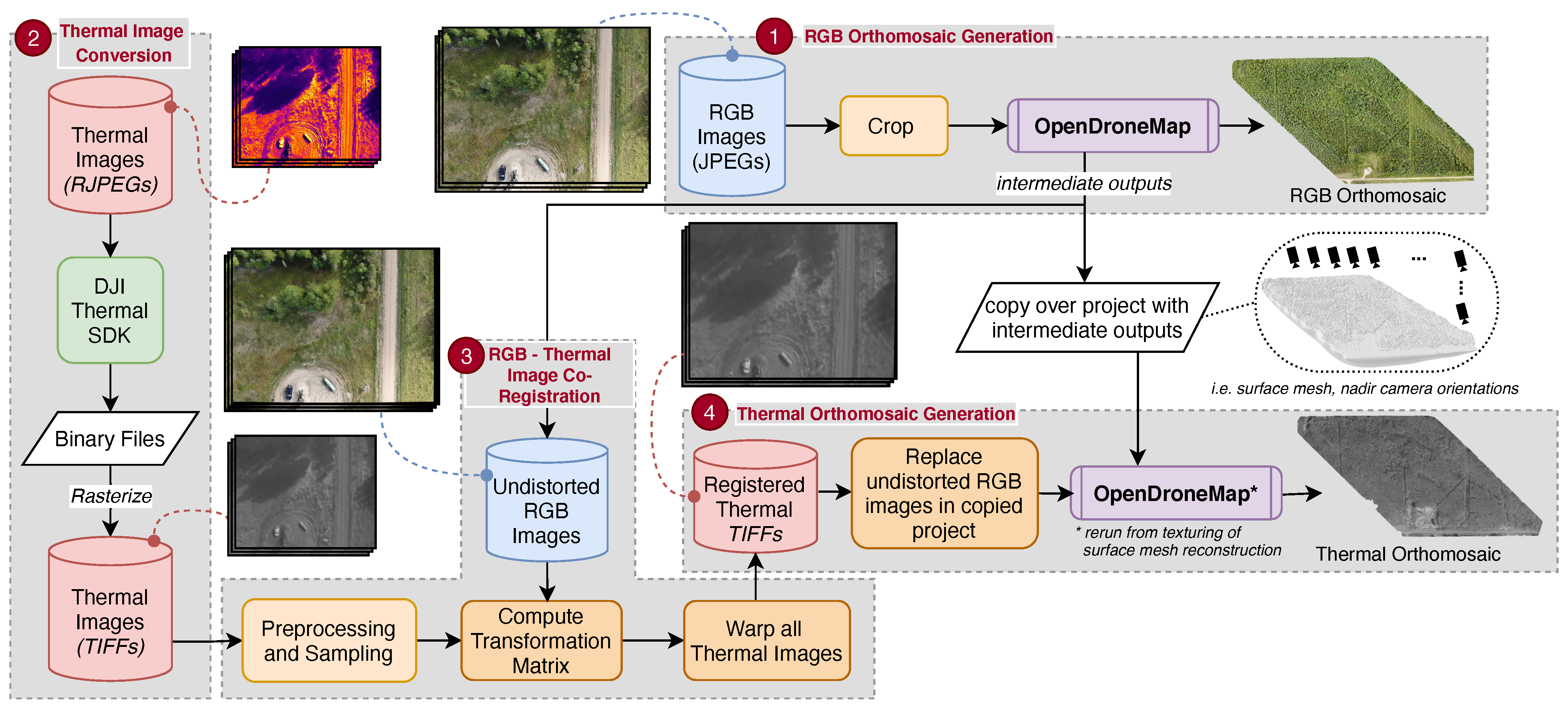
The proposed integrated orthomosaicking workflow comprises four stages, as shown in Figure 3: (1) RGB orthomosaic generation, (2) thermal image conversion (from R-JPEG to grayscale TIFF), (3) RGB–thermal image co-registration, and (4) thermal orthomosaic generation. The proposed workflow has also been implemented as an open-source tool, which is presented with more details in Section 2.4.
The rest of this section provides a brief summary of our integrated workflow, and the following subsections describe each stage in more detail. In the first stage, ODM is used to generate an RGB orthomosaic. This relies on structure from motion (SfM) [22], a computer vision process that automatically aligns the overlapping drone photos. After this, a dense point cloud and a surface mesh of the study area are derived together with the estimated camera orientations, as shown in the dotted bubble on the right side of Figure 3. Undistorted RGB images are also obtained as intermediate outputs—these are the original input RGB images, but are corrected for radial and tangential distortions. After the RGB orthomosaic is generated, we duplicate the ODM project along with its intermediate outputs and replace the undistorted RGB images with thermal ones, which are created in the following two stages.
In the second stage, we preprocess the thermal images to obtain, out of the native R-JPEG format, a single-channel (i.e., grayscale) image that displays the surface temperature of each object. In the third stage, we compute the transformation matrix that co-registers every preprocessed thermal image with its corresponding undistorted RGB image, such that both are geometrically aligned and objects appear in the same pixel locations in both. Note that this geometric alignment (i.e., co-registration) is different from the ‘alignment’ during SfM, which yields the external orientations of the cameras.
Finally, in the fourth stage, we replace the undistorted RGB images in the duplicate of the ODM project with the co-registered thermal images obtained from the previous stage and restart the ODM process from the texturing step. In this way, we avoid using any thermal images for SfM. Instead, we only use the co-registered thermal images to texture the surface mesh previously derived from the RGB images during the first stage. This stage outputs a high-quality thermal orthomosaic that is geometrically aligned with the RGB orthomosaic.

2.2.1. RGB Orthomosaic Generation

In the first stage of our proposed workflow, we use ODM to generate the RGB orthomosaic of the study site from the collected RGB nadir drone images. If the FOVs of the RGB and thermal cameras differ drastically, such as for the H20T instrument, the central regions of the RGB images are cropped so that each RGB–thermal pair depicts roughly the same scene. This is necessary for effective geometric alignment in the RGB–thermal image co-registration stage later on. The exact amount of cropping depends on the specific cameras used. In general, the cropping must maintain sufficient forward and sideways overlap between adjacent images for effective orthomosaicking. In our case, we crop the 3040 × 4056 wide-angle RGB images to 1622 × 1216 pixels (60% reduction in width and height). An additional advantage of cropping wide-angle RGB images is that it mitigates lens distortion from the edges of such images from propagating to the orthomosaic. Without cropping, relief displacement (tree lean) effects would likely occur in the RGB orthomosaic due to the relatively low flight height [23]. Moreover, reducing the image size by cropping enables faster processing in ODM. Once the RGB orthomosaic is successfully generated by ODM, we duplicate the project to be used in later stages.
The key steps involved in the orthomosaic generation process of ODM are summarized as follows. The 3D structure of the area of interest (AOI) is reconstructed using the SfM technique within ODM, namely OpenSFM [43]. This involves extracting tie points (corresponding to salient features) from images using the scale-invariant feature transform algorithm [44] and then matching tie points from overlapping images. These points are then located in 3D space using parallax. Next, the external orientation of the camera for each image is refined in an iterative process called bundle adjustment. Finally, new points are added to the initial point cloud of tie points using a process called multiple view 3D reconstruction based on depth maps [45], yielding a dense point cloud with thousands of points per square meter.
The SfM process additionally performs internal camera calibration, providing estimates for the focal length, principal point, and distortion coefficients of the camera model. The same internal camera parameters apply to all RGB images, since they are all captured by the same sensor. The estimated distortion coefficients are used to undistort every individual RGB image under the Brown–Conrady distortion model [46]. This models the radial distortion in the RGB images using coefficients k 1 , k 2 , and k 3 , and tangential distortion with coefficients p 1 and p 2 , both arising from the camera lens shape. Briefly, every pixel location in the original image is mapped to its corresponding location in the undistorted image, meanwhile correcting for the distortions using these coefficients. More details about the exact formulation can be found in [46]. Compared to the (distorted) image taken from the wide-angle lens, the undistorted image is warped to look closer to what it would look like using a pinhole camera. For instance, straight lines in the real world that appear curved in the captured image are recovered as straight in the undistorted image.
OpenMVS [47] is then used to produce a textured mesh with the undistorted images: outliers in the dense point cloud are filtered out, and the 2.5-dimensional surface mesh, i.e., a warped surface typically made of small triangles that represents the outer envelope of the point cloud, is generated using Screened Poisson Reconstruction [48]. At this point, the estimated external orientations (one for each image) and camera internal parameters (same for all images) are used to determine how to texture the triangular mesh surfaces, which involves selecting for each small triangle the undistorted image from which it is best observed. This is performed through Triangle to Image Assignment, whichs takes into account each image’s proximity to the triangle, the triangle’s amount of occlusion (if any), and the viewing angle’s steepness relative to the triangle surface [42]. Once assigned, the relevant pixels of the undistorted images are projected on to the triangular surfaces using the calculated transformation matrices from the exterior and interior parameters. Finally, the orthomosaic is generated as the orthographic projection of the textured mesh onto the horizontal plane defined by the chosen coordinate system (NAD83 UTM 12 N in our case). The default ground sampling distance (GSD) corresponds to the average pixel size on the mesh surface. In our case, we rounded GSD up to 5 cm. This results in a single, high-resolution RGB orthomosaic of the study area. This texturing-based orthomosaicking is different from alternative methods that use a digital surface model to orthorectify individual images that are later stitched together.

2.2.2. Thermal Image Conversion

The 3-channel, 8-bit RJPEG images captured by the H20T camera, which are intended for visualization (as in the top left of Figure 3), are converted to absolute surface temperature readings in degrees Celsius and stored as 32-bit floating point TIFF images. This is performed through the DJI Thermal SDK (software development kit) using the ‘measure’ functionality, with average emissivity as 0.95 and distance to target as >25 m for all flights. Relative humidity and reflected temperature (i.e., air temperature) are set independently for each flight using the values reported in Table 1. The SDK outputs one binary file for each image, which are then rasterized into grayscale TIFF images such as those in Figure 3.

2.2.3. RGB–Thermal Image Co-Registration
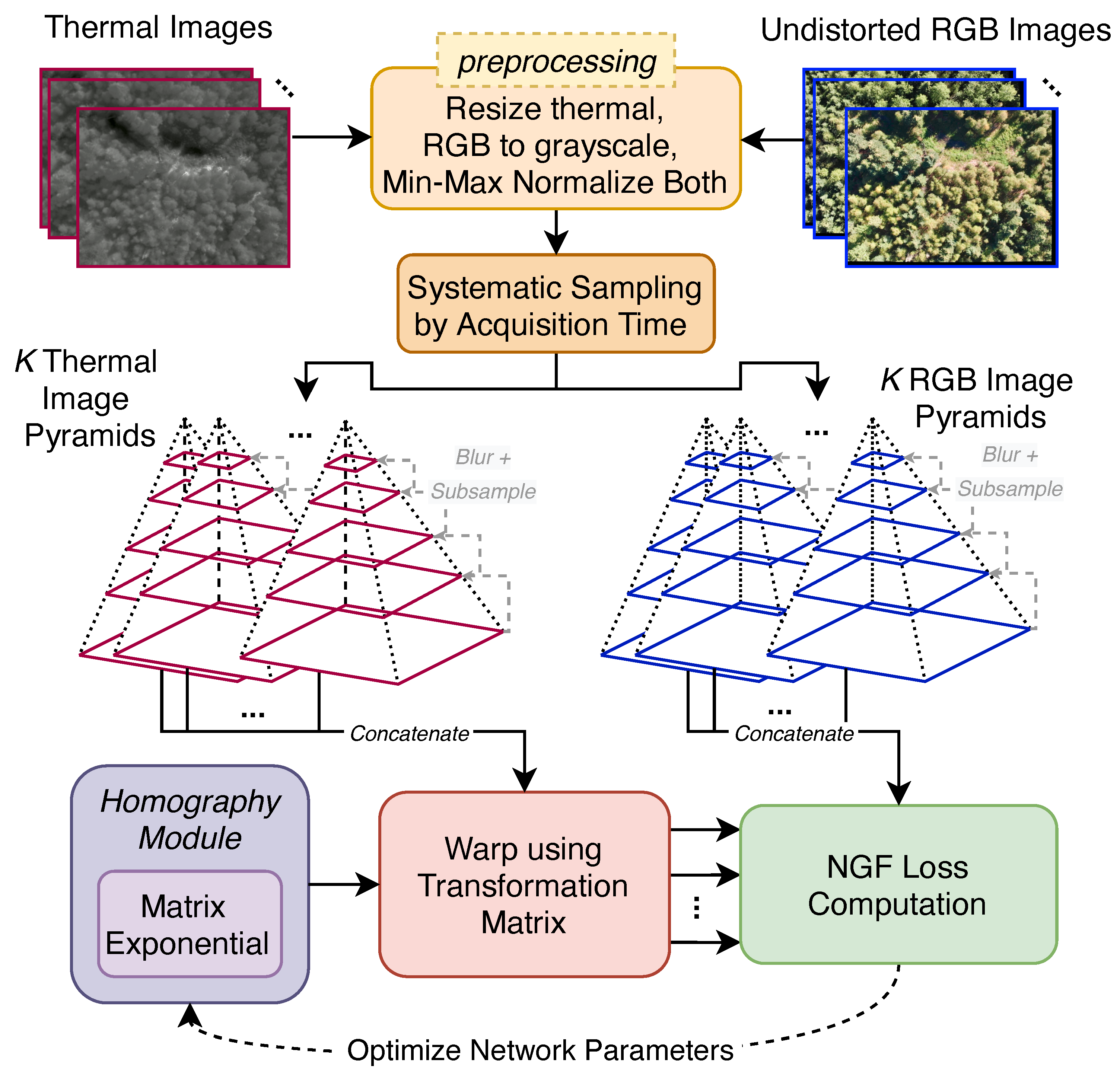
As a result of the initial cropping of the RGB images, the footprint of a preprocessed thermal image roughly coincides with that of its corresponding undistorted RGB image. In this stage, the geometry of the image pairs is more precisely aligned through image co-registration. Specifically, we compute an estimate to the optimal geometric transformation matrix M * that co-registers every thermal image with its corresponding undistorted RGB image, such that objects appear in the same pixel locations in both. In this work, we compute a single affine linear transformation matrix, i.e., a 3 × 3 matrix with 6 degrees of freedom that preserves parallel lines. The same transformation applies to all image pairs as they all come from the same instrument that simultaneously captures both modalities. This has the advantage of being computationally efficient while not adversely impacting co-registration performance, as we will demonstrate in Section 3. Once we have a close approximation to the optimal M * , we use it to warp all the thermal images to emulate their undistorted RGB counterpart, using the concept of inverse warping [49]. For every pixel location ( x o u t , y o u t ) in the warped output thermal image, the pixel location ( x i n , y i n ) in the input thermal image is obtained by performing matrix multiplication of the inverse of M * with the homogenous coordinates ( x o u t , y o u t , 1 ) T . Note that the third dimension is used to scale coordinates in the projective plane and set by convention to 1. Then, we assign the value at the pixel location ( x i n , y i n ) in the unwarped image to ( x o u t , y o u t ) in the warped image, performing re-sampling through bicubic interpolation.
In this work, we investigate two methods for computing the optimal transformation matrix M * . One is to manually supply up to four-point correspondences between a pair of RGB and thermal images, and then to solve a system of linear equations for an estimate of M * [50]. Although these correspondences need to only be supplied once, the quality of co-registration (and optimality of the computed transformation matrix) heavily depends on their correctness.
In the second method, M * is automatically computed through intensity-based image co-registration using gradient descent optimization, inspired by [37,38]. Given a set of N thermal images and their corresponding N RGB counterparts, we compute an approximation to the optimal transformation matrix M * that aligns the geometry of the pairs. The gradient descent optimization iteratively refines the 6 learnable parameters (i.e., variables) within a Homography Module that encapsulates the computation of the transformation matrix M [37]. We use intensity-based co-registration, which does not rely on extracting features from both images, working instead directly with the pixel values and image gradients [38]. Figure 4 summarizes this process, and a detailed description follows below.
First, both sets of images need to be preprocessed to facilitate further computations. We resize the grayscale thermal images extracted during the previous stage by upscaling through bicubic interpolation to match the dimensions of the undistorted RGB images (i.e., from 640 × 512 to 1622 × 1216). We then min–max normalize the resized thermal images. As for the undistorted RGB images, we convert them to a single-channel luminance representation using the weighted formula L ( x , y ) = 0.2125 R + 0.7154 G + 0.0721 B for each pixel location ( x , y ) , as defined in the rgb2gray function of the scikit-image processing library [51]. We also min–max normalize the resulting grayscale images.
Figure 4. Steps involved in our automated intensity-based image co-registration. After preprocessing the images, K RGB and thermal image pairs are systematically sampled for batch processing. The parameters of the Homography Module [37] represent the values in the transformation matrix being computed and are learned during gradient descent optimization [52] of the normalized gradient fields (NGF) loss [53] between each transformed thermal Gaussian pyramid and its corresponding RGB pyramid.
Remotesensing 15 02653 g004
The gradient descent-based optimization is a computationally intensive process. To avoid loading all image pairs into the hardware memory (CPU or GPU) while still ensuring the transformation matrix computation is robust, we sample a batch of 64 image pairs, which we deemed sufficient after empirically testing different batch sizes. Furthermore, working with a batch rather than a single pair ensures less variance in gradient calculations while encouraging good convergence during gradient descent [52]. Although any image pairs can be selected for the batch as we are trying to compute a single linear transformation matrix that applies to all pairs, appropriately choosing batch pairs is important for good co-registration performance. We, therefore, perform systematic sampling: the RGB–thermal image pairs are first ordered by acquisition time and every j-th pair is selected for the batch, where j = N / K and K is the batch size. Besides the intuitive reasoning that the computed M should be more robust due to more complete coverage of the AOI within the batch, our quantitative results will also show that systematic sampling is preferable to random sampling for batch pairs. A multi-resolution Gaussian pyramid is then constructed for all the grayscaled, normalized RGB and thermal image pairs in the batch, where each smaller layer is obtained by blurring followed by sub-sampling from the previous larger one [39]. We utilize a batch size of 64, with 11 levels in each pyramid at a downscale factor of 1.5. Blurring is performed with a filter mask twice the size of the downscale factor that covers more than 99% of the Gaussian distribution, and sub-sampling is performed through pixel averaging. This multi-resolution framework ensures that the current estimate of M will be refined simultaneously at multiple scales, allowing for more precise and robust co-registration [54].
During gradient descent, the following objective function is optimized to find the transformation matrix M that warps every thermal image T to most closely align its geometry with that of its corresponding RGB image R [37],
min M L ( R , W a r p ( T , M ) ) ,
where L is the normalized gradient fields (NGF) loss function [53]. This loss function is well suited for optimization and is also preferable for multi-modal images [38]. It is based on the principle that two images are well-registered if intensity changes occur at the same locations. NGF computation requires the x-direction gradient ( x I ( x , y ) ) and y-direction gradient ( y I ( x , y ) ) of the image I at every pixel location ( x , y ) , which we numerically approximate using central finite difference [55],
x I ( x , y ) I ( x + 1 , y ) I ( x 1 , y ) 2 , y I ( x , y ) I ( x , y + 1 ) I ( x , y 1 ) 2
Then, the NGF loss L ( I , J ) for two grayscale images I and J as in [38],
L ( I , J ) = 1 w h x = 1 w y = 1 h [ ( x I ( x , y ) I ( x , y ) x J ( x , y ) J ( x , y ) ) 2 + ( y I ( x , y ) I ( x , y ) y J ( x , y ) J ( x , y ) ) 2 ] ,
where h and w are the numbers of rows and columns in both images, and I ( x , y ) denotes the point-wise gradient magnitude at pixel ( x , y ) .
For the gradient descent-based optimization to work, M is encapsulated as the learnable parameters v within a simple differentiable module, termed the Homography Module [37], using the matrix exponential representation [56],
e x p ( A ) = k = 0 A k k ! .
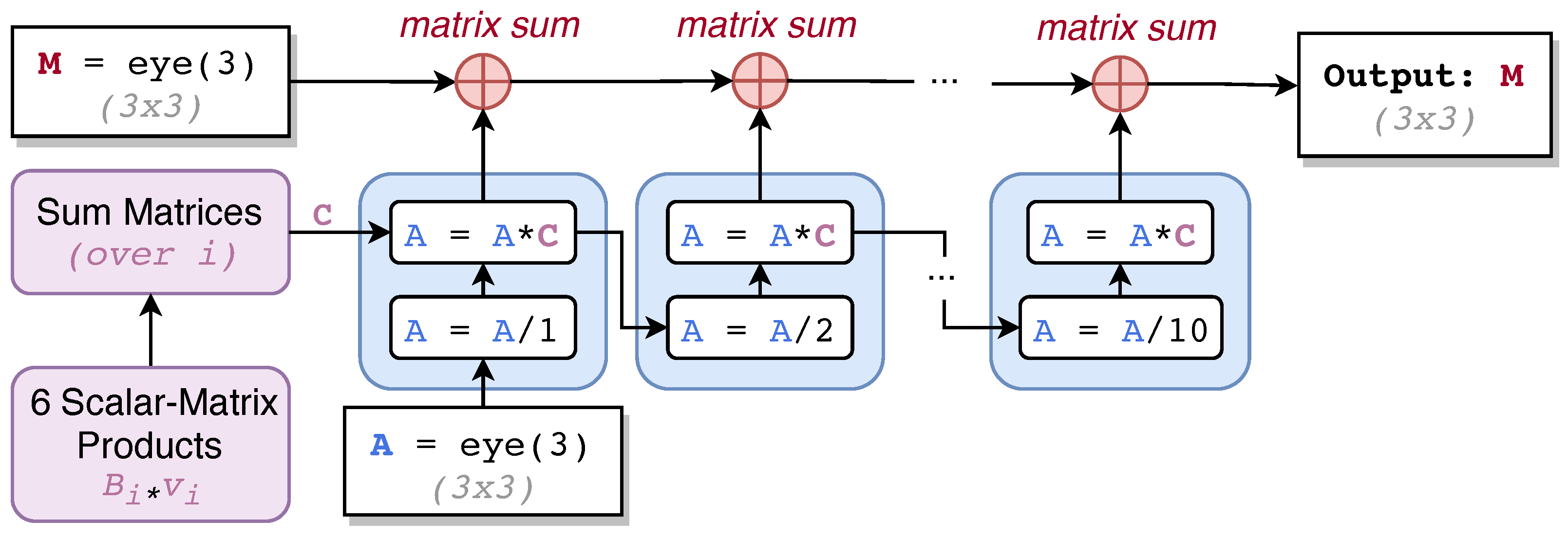
The matrix exponential formulation has the following two desirable properties [40]. Its computation is differentiable, which is necessary for learning the Homography Module’s parameters v through backpropagation during the gradient descent optimization. Moreover, the output of the matrix exponential function (i.e., the computed transformation matrix) is always invertible, so we can reliably combine forward and inverse transforms for more robust NGF loss computation. In practice, using 10 terms closely approximates the sum of the infinite series. Using the matrix exponential representation, the objective function in Equation (1) can be rewritten as
min v L ( R , W a r p ( T , M ( B , v ) ) ) ,
M ( B , v ) = e x p ( i = 1 6 v i B i ) ,
where M ( B , v ) is the current estimate of the affine transformation matrix, derived from the current parameters v = { v i | i = 1 , , 6 } of the Homography Module and the constant basis matrices B = { B i | i = 1 , , 6 } . These 3 × 3 matrices are generators of the group of affine transformations on the 2D plane, as described in [37]. Therefore, any affine transformation matrix may be computed using this formulation. Before commencing training, we initialize v i = 1 for all i = 1 , , 6 . Figure 5 summarizes the mechanism of the Homography Module and how the matrix exponential is implemented within it.
At every step of the optimization loop in Figure 4, the current parameters v of the Homography Module are used to derive M. Using M, we compute the average NGF loss between RGB and warped thermal pairs (forward transform loss), as well as between thermal and warped RGB pairs (inverse transform loss) at every image pyramid level and sum both losses. The total multi-resolution loss is the sum of bi-directional losses over all levels of the pyramid. Backpropagation [57] is used to learn the parameters within the Homography Module v by using the partial derivatives with respect to v of the computed multi-resolution NGF loss to adjust v in a way that decreases loss. We utilize the Adam optimizer [58] (as implemented in the PyTorch software library [59]) with a learning rate of 0.005. All other optimizer hyperparameters are unchanged from their defaults. After each training iteration, the computed loss should decrease and the estimates of v should be closer to their optimal values. Training is terminated once convergence is reached (i.e., loss stops decreasing), for which we found 200 iterations to be sufficient during all our experiments. At this point, the best approximation to the optimal transformation matrix M * has been found. In the final step of this stage, we use M * to warp all the resized, non-normalized thermal images. We warp the non-normalized images because we want to preserve the original absolute temperature values during orthomosaicking in the next stage.
Note that the described intensity-based co-registration we utilize is different from previous feature-based registration techniques that match salient feature descriptors between the images, for example in [32]. It is also different from the mutual information (MI)-based registration in [37], which trains an additional neural network to approximate MI for image pairs as a measure of similarity of their gray-level histogram distributions, and performs gradient descent with respect to MI loss to compute the transformation matrix for registration. They consider pixels that belong to edges (determined by Canny edge detection) to compute MI, but we use all pixels in our intensity-based registration to compute NGF loss, since we observed Canny edge detection to not be robust for the aerial forest images in our dataset. Lastly, in comparison to the pair-specific diffeomorphic (non-linear) transformations used in [38] for medical image registration that deforms images unevenly, we restrict the computation to a single linear transformation matrix for all image pairs, which is both efficient and effective for our work as our results will corroborate.

2.2.4. Thermal Orthomosaic Generation

In the final stage of our proposed workflow, we first replace the undistorted RGB images in the duplicate of the RGB orthomosaic project with the co-registered thermal images obtained from the previous stage. Then, we rerun this duplicated ODM project starting from the texturing step. The same external camera orientations estimated from the RGB SfM process during orthomosaicking are reused here. As a result, the co-registered thermal images are used to texture the surface mesh previously obtained as an intermediate output of the RGB orthomosaicking process. In this way, ODM outputs a thermal orthomosaic. Because the individual undistorted RGB and thermal images were co-registered in the previous stage, the RGB and thermal orthomosaics are also co-registered (i.e., geometrically aligned)—each tree appears at the same pixel locations in both orthomosaics. Both orthomosaics also contain the same georeferencing information, and hence they line up exactly when viewed using GIS software (see the next section).

2.3. Downstream Tree Crown Detection Task

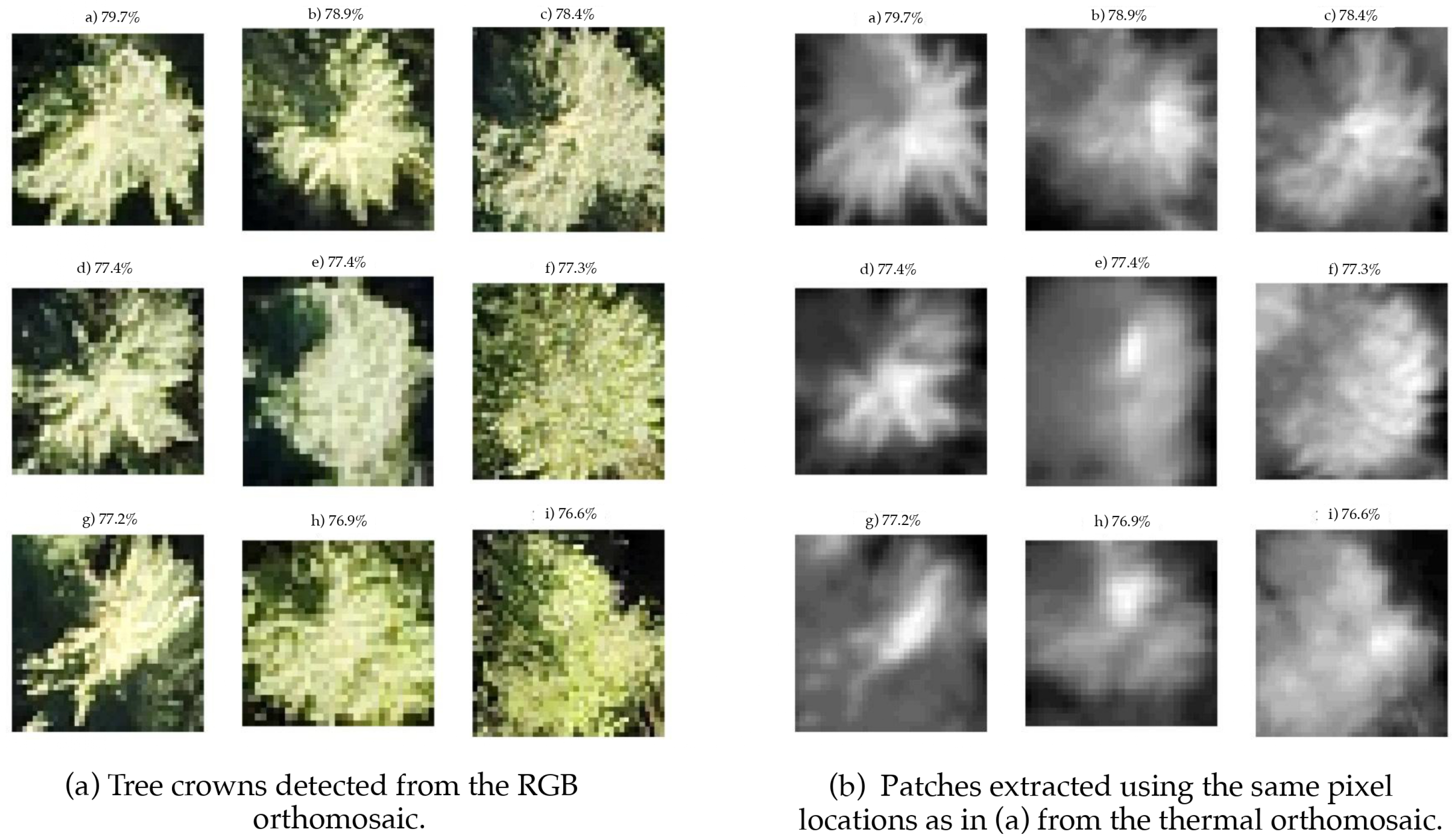
To highlight the versatility and utility of the proposed workflow, we will demonstrate how the generated orthomosaics can be used for a practical downstream task, specifically tree crown detection. We will use DeepForest [41], a pre-trained deep neural network, to delineate individual tree crowns from the RGB orthomosaic. This model was pre-trained using RGB images, not thermal ones. However, since our workflow generates geometrically aligned orthomosaics, our results in Section 3.5 will show that the same bounding boxes obtained from the RGB orthomosaic apply directly to the thermal orthomosaic generated from our proposed workflow.
The DeepForest network is based on the one-stage object detection RetinaNet [60] framework. Its backbone comprises a ResNet-50 [61] neural network that extracts multi-scale features from the image, and a feature pyramid network (FPN) [62] that combines semantically low-resolution features with low-level, high-resolution ones. Each level of the FPN feeds its computation to a regression head that locates bounding boxes in the image and to a classification head that outputs a confidence score for each box. This score denotes the model’s confidence that a tree crown is contained within the predicted box.

2.4. Proposed Open-Source Tool

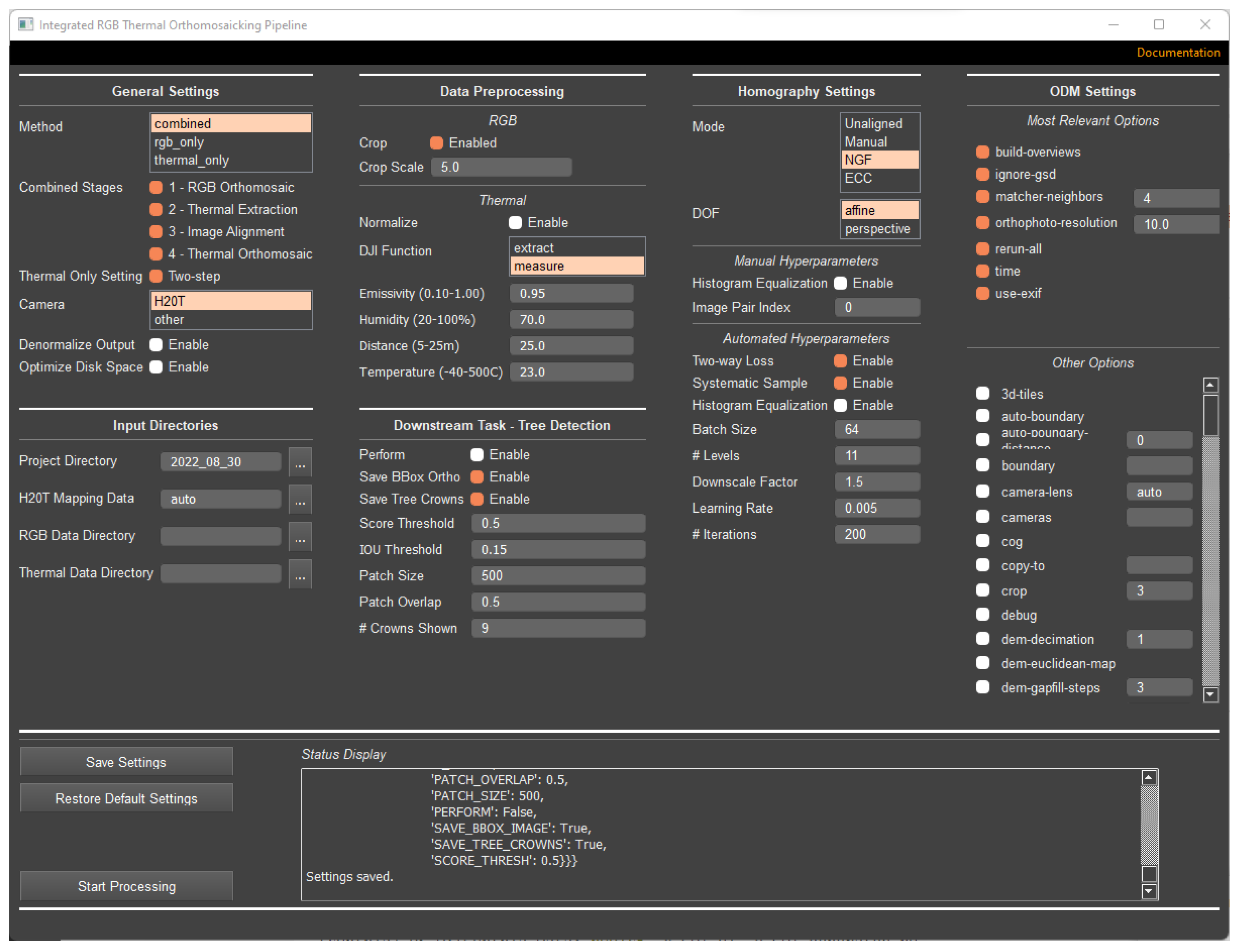
To facilitate the usage of our proposed workflow, we have created an open-source tool that offers both a command line interface and a graphical user interface (GUI) that was developed using the PyQt5 Python library. As shown in Figure 6, every setting for each stage of our workflow can be easily customized from the GUI depending on the specific requirements of a project. The tool runs on the Windows operating system. It leverages GPU acceleration if a graphics card is available. The tool offers the option to toggle each processing stage, including the downstream tree detection, and to specify their relevant hyperparameters. For example, it is possible to specify the batch size, the number of pyramid levels, and the degrees of freedom in the co-registration stage. Additionally, there is an option to either supply manual point correspondences for a chosen image pair or to compute the transformation automatically using the described intensity-based co-registration. The tool also offers the option to select RGB-only or thermal-only processing.

2.5. Performance Assessment

We generate all orthomosaics at a ground sampling distance (GSD) of 10 cm, which is close to the spatial resolution of the original thermal images taken at nadir. The drone images used are those collected from the Cynthia cutblock, as described in Section 2.1. Although we used the same H20T camera for all flights, we compute separate transformation matrices for the geometric alignment of each flight individually. We compare the quality of four different co-registration techniques on individual thermal and RGB image pairs. The first is the baseline, i.e., not performing any co-registration of thermal and RGB images, similar to that in [25]. The second is manual co-registration, where an affine transformation matrix is computed using three-point correspondences supplied manually by a user when looking at a randomly chosen RGB–thermal pair, similar to that in [27]. We conducted 10 repeated trials and report the best result obtained. The third technique is our proposed intensity-based registration framework using the NGF loss function, as described in Section 2.2.3. For the fourth, we simply replace NGF with the enhanced correlation coefficient (ECC) [28] as the loss function in our proposed workflow. ECC seeks to maximize the pixel-wise correlation between image pairs and has been used in previous works for RGB–thermal co-registration [29,30,31]. We compare these techniques using mutual information (MI) as a quantitative metric, which measures how well the intensity in one image can be predicted given the intensity in the other. Thus, it can be used to measure the similarity in gray-level distributions for two images using their histograms. We also use MI in further experiments to determine the optimal design choices for other parts of our proposed workflow, such as batch size for sampling. We then present qualitative comparisons by displaying the co-registered images and orthomosaics of the unregistered baseline and our proposed NGF-based workflow. Additionally, we use the Bhattacharyya coefficient [63] to compare the histograms of randomly chosen original thermal images and their corresponding patch in the thermal orthomosaic to show that our workflow preserves radiometric information in the form of absolute temperature values. We then present the performance of the downstream tree crown detection task on the thermal orthomosaics using the RGB-detected tree crowns, and finally provide information on the processing times of our workflow. The observed results are discussed in Section 4.

3. Experimental Results

3.1. Quantitative Results

Typically, image registration techniques are evaluated against a ‘gold standard’ registration using a measure of positional error between known ground truth correspondence points when available [64]. However, we do not have this information for our study site for the two modalities, as many of the image pairs lack any salient geometric feature to be used as ground truth. Specifically, points on swaying tree crowns due to wind are not suitable, and easily identifiable hotspots in thermal images do not necessarily correspond to salient features in the RGB images (and vice versa). Therefore, we propose to use the MI between an RGB and thermal image pair as a quantitative metric to measure the performance of each image co-registration technique. Better co-registration corresponds to a higher MI value. For all image pairs, we compute MI using the histograms of the min–max normalized images with 100 equally spaced bins, as described in [37].
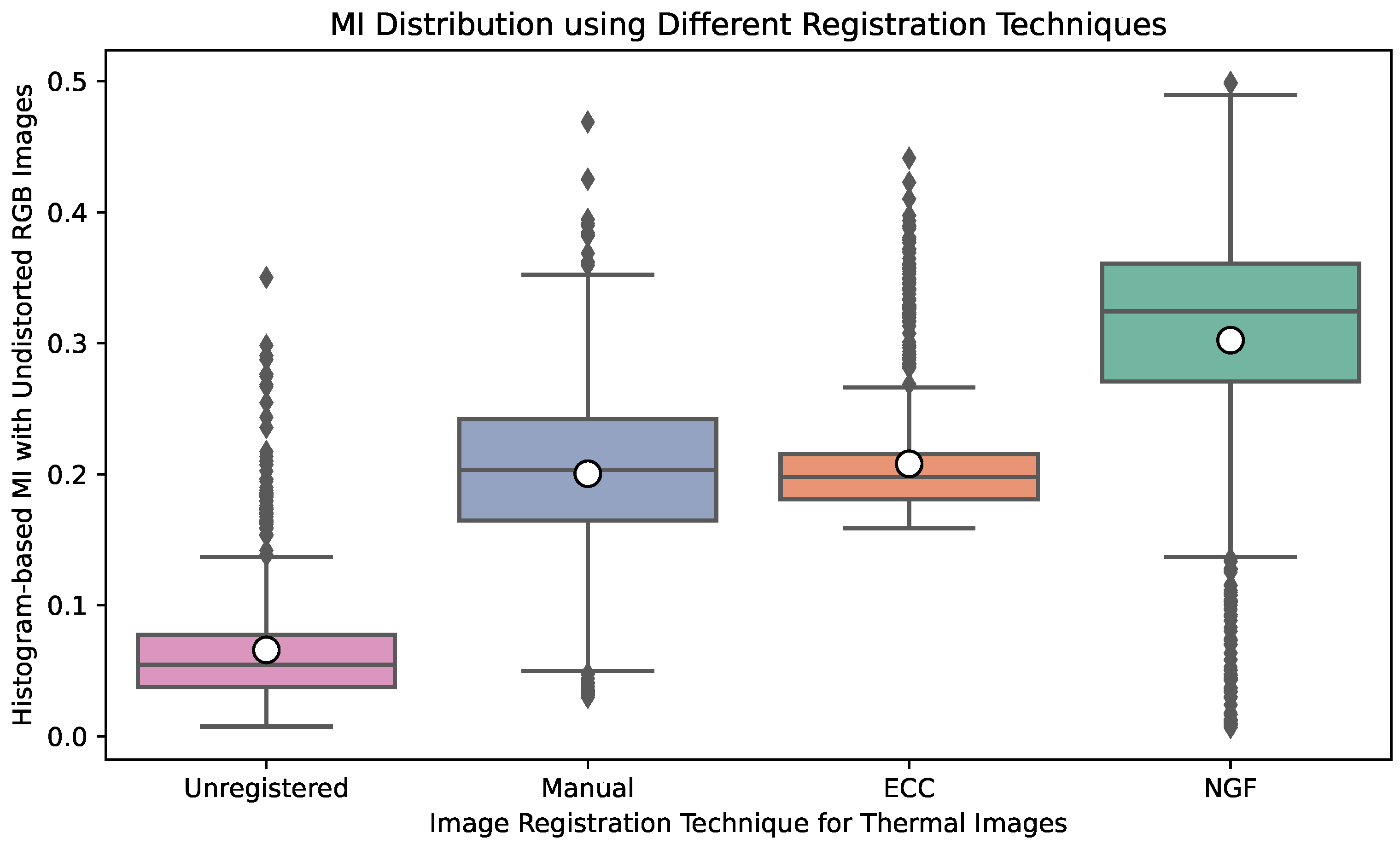
Figure 7 shows the MI between the individual RGB and thermal images from the August 30 Cynthia flight. The unregistered images have a median MI of 0.054. Performing manual image co-registration improves the median MI of the image pairs to around 0.203. Although this is a considerable improvement, it could be even higher if more accurate point correspondences are provided. The transformation matrix computed automatically using intensity-based co-registration with NGF as the loss function results in the highest MI, with a median value of 0.324. Using ECC in place of NGF produces a significantly lower median value of 0.198, close to the performance achieved by manual registration. Except for July 26 where ECC performs slightly better than NGF, similar results in terms of relative performance were obtained for the other flights (Table 2). These results indicate that the intensity-based co-registration using NGF most closely aligns the geometry of the RGB and thermal images compared to the other co-registration techniques.
In Table 2, we report the average MI from co-registering all individual thermal and RGB images using different design choices within our proposed workflow. There is one column for each flight in the Cynthia cutblock data, and the final column reports the arithmetic mean over all five flights. The rows are divided into multiple sections, one for each design choice. Each design choice is tested independently while setting all others to their best-performing options (indicated in bold). We make the following observations from the reported results: (1) Co-registration using NGF outperforms the other techniques on average over the 5 flights by 0.2196 units over unregistered, 0.0853 units over ECC, and 0.0575 units over manual. (2) Restricting the transformation matrix to six degrees of freedom (affine) results in a slightly higher average MI than allowing eight degrees of freedom (perspective). (3) The multi-resolution Gaussian image pyramid framework performs immensely better than using only the single highest-resolution image by 0.2519 units. (4) Using larger batches leads to higher average MI, with a batch size of 64 yielding the most performance improvement by least 0.02 units over smaller batches. Finally, (5) systematically sampling image pairs for the batch marginally improves performance compared to choosing pairs randomly. Setting each design choice to its best-performing option yields the highest average MI of 0.2787, indicated in bold. In comparison, the average MI between the perfectly registered red and blue channels of the same RGB images from the August 30 flight is 1.4896, which is predictably higher than the reported values between grayscaled RGB and thermal pairs of different modalities.

3.2. Qualitative Results

The quality of the generated thermal orthomosaic depends on the accuracy of the geometric alignment between the individual RGB and thermal images. If the co-registration is poor, some tree crowns tend to appear twice while others are missing from the orthomosaic. Additionally, objects tend to not line up correctly. Figure 8a shows the RGB orthomosaic generated for the Cynthia cutblock from the August 30 flight. Figure 8b shows the orthomosaic obtained by texturing using unregistered thermal images. Although there are no gaps (similar to the RGB orthomosaic), the poor quality of this thermal orthomosaic is noticeable from the jagged nature of the vertical paths through the trees (cutlines). Using the co-registered images obtained after applying the transformation matrix computed with NGF and the other best-performing design choices denoted in Table 2, a higher quality orthomosaic is generated, as shown in Figure 8c. The cutlines are straight, and no individual trees are missing or duplicated.
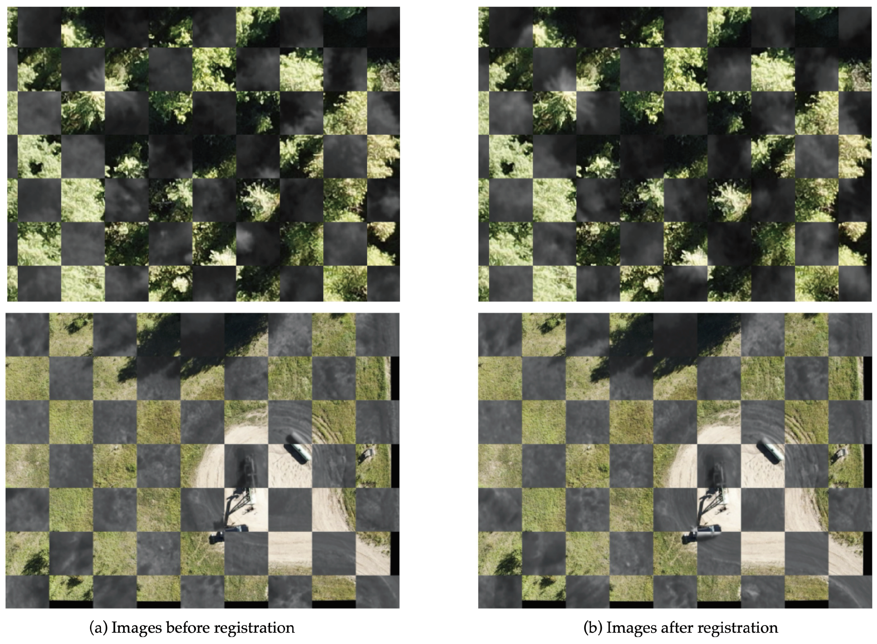
The co-registration performance can also be observed by interlacing an undistorted RGB image with its corresponding thermal image before and after co-registration, as shown in Figure 9. Prior to co-registration, there is an offset between the images that is especially noticeable from the larger individual trees in the top row, as well as from the road and parked vehicles in the bottom row. The geometric alignment of the two images significantly improves after co-registration. This explains why our co-registration technique results in a higher quality orthomosaic when the images are used to texture the surface mesh reconstruction. Because of the geometric alignment of the individual RGB and thermal images, the resulting orthomosaics are also geometrically aligned.

3.3. Robustness of Transformation Matrix Computation

As mentioned previously, we compute five separate transformation matrices for performing co-registration, one for each of the five flight dates. Since the same H20T instrument is used across all flights, the computed transformation matrices are expected to be identical in theory. In practice, variations may arise due to differences in lighting conditions during the times of data acquisition, for example. Table 3 reports statistics of the average, minimum, and maximum values of each component of the affine transformation matrices computed for all five flights. The maximum coefficient of variation (CoV) is observed to be 33.69% for M 2 , 1 (the component that controls vertical shear). Despite this high relative value, the maximum absolute difference from the average for this component across the 5 flights is merely 0.00536, and therefore leads to a minor impact on the final transformation. For instance, with the point (400, 300) in the original image (approximately the middle point between the image center and top left corner), applying the 3 × 3 transformation matrix corresponding to the highest value of M 2 , 1 yields the point (390.36, 269.04). On the other hand, applying the matrix with the smallest value of M 2 , 1 yields (391.74, 266.85). The Euclidean distance between these 2D image points is just 2.59 pixels, or around 13 cm on the ground. This confirms that our co-registration workflow is robust, with only minor differences in the computed transformation matrices across different flights.

3.4. Radiometric Analysis

Here, we show that our workflow preserves the radiometric information present in the individual thermal images that are used to generate the orthomosaic. Specifically, we show that the captured absolute temperature values are the same before and after orthomosaicking for any given region. Figure 10 shows the central 256 × 204 pixel region of a sample thermal image and its corresponding patch (of the same size) extracted from the thermal orthomosaic generated by our workflow. Cropping for this experiment is performed to ensure the orthomosaic patch corresponds to only this single image, as the texture mapping tends to only use the central portion of images during orthomosaic generation. It also shows that their temperature histograms (in bins of 0.1 °C) are nearly identical. The level of similarity between the histograms can be quantified using the Bhattacharyya coefficient [63], which measures overlap between two statistical populations. For 50 randomly chosen thermal images across all 5 flights, the average Bhattacharyya coefficient with their corresponding orthomosaic patches is 0.992 (minimum 0.984, maximum 0.998). This is very close to the theoretical maximum value of 1. Therefore, our orthomosaicking workflow successfully preserves radiometric information, i.e., absolute temperature values.

3.5. Downstream Task Performance

Figure 11a shows some examples of the detected tree crown patches from RGB orthomosaics using the DeepForest pre-trained tree crown detector. The confidence score of each prediction in the figure is greater than 75%—there is only one tree centered tightly within each patch. In total there were 8729 trees detected with confidence over 50%. We use the same bounding box coordinates on the thermal orthomosaic, and the patches are shown in Figure 11b. As a result of the good geometric alignment between the generated orthomosaics, the same trees appear in each of the corresponding pairs at the same locations. Hence, the proposed workflow enables applying an external model trained solely on RGB images to correctly detect individual tree crowns from the generated thermal orthomosaic from our workflow.

3.6. Processing Time

The CPU-only processing time for 814 RGB images (cropped to 1622 × 1216) and 814 thermal images (640 × 512) for the August 30 flight through all stages of the proposed workflow was around 2 h and 25 min (with around 75 min for co-registration). This result was for a machine running on a 12th Generation Intel Core i9-12900 K 3.19 GHz processor with 32 GB of RAM. With a single NVIDIA GeForce RTX 3090 GPU, the total time was reduced to around 80 min. The bulk of this processing time is taken up by the ODM process with RGB images for obtaining the surface mesh and undistorted RGB images. The co-registration stage takes just around 10 min.

4. Discussion

The quantitative results reported in Section 3.1 emphasize the importance of choosing the correct hyperparameters during the RGB–thermal image co-registration stage. Automated intensity-based co-registration through gradient descent of the NGF loss function on average outperformed the other co-registration techniques, owing to its suitability for gradient descent optimization and multi-modal data [38]. Using ECC as the loss function resulted in a higher MI for one of the flights (July 26), but overall it performed poorly compared to using NGF. This indicates that ECC as a loss function in our proposed workflow is not as robust to different data as NGF for co-registering RGB and thermal drone images of forests. Manually supplying point correspondences for co-registration performed slightly better than ECC but worse than NGF, possibly due to human errors in selecting the exact pixels for correspondence. These errors stem from the possibility that hotspots (i.e., bright points) in a thermal image may not correspond to easily identifiable features in the RGB counterpart, and vice versa. Regarding the transformation matrix, restricting it to six degrees of freedom (affine) yielded a slightly better mean MI than allowing all eight degrees of freedom (perspective). This is because the RGB and thermal sensors lie on the same plane (or at least parallel planes) in the drone instrument, and both capture nadir images. Hence, there is only a variation in the scale and translation, with possible rotation and skew between the two sets of images [32]. Allowing the two additional degrees of freedom in perspective transformation matrices led to a non-zero level of warping in the z-direction (perpendicular to the image plane). While this did not significantly reduce MI (and actually increased MI for the August 30 flight), we observed that it introduces a regular pattern of distortion in the generated orthomosaic due to the misalignment of the image planes. Hence, our proposed workflow only considers affine transformation matrices.
The quantitative results further show that using a multi-resolution Gaussian pyramid framework is essential for proper co-registration—only relying on the single-scale original image significantly deteriorated performance even compared to the unregistered images. This is consistent with previous research showing that multi-resolution frameworks are beneficial for image registration [54]. It can also be seen from our results that batch processing consistently outperformed single-image processing due to the computation of average gradients during optimization that reduces variance and promotes good convergence [52]. Using larger batch sizes increased performance for all flights, and although a batch size of 16 or 32 yielded competitive results with a size of 64, the latter option performed the best on average across all flights. Finally, our results corroborate the intuition that systematic sampling of image pairs for batch processing offers a good starting point for successfully performing co-registration. Compared to random selection, systematic selection was more robust, resulting in a slightly higher mean MI value. Overall, the reported results justify the specific design choices of the intensity-based co-registration stage within our proposed integrated workflow by demonstrating the robustness and high performance of the automated co-registration using the NGF loss function, multi-resolution image pyramid framework, batch processing, and systematic sampling. In our experiments, we achieved the highest MI of 0.2787 by using this co-registration framework. This may seem low compared to the average MI of 1.4896 for the blue and red channels of the undistorted RGB images. However, this can be explained by the fact that thermal and RGB images carry very different information, so the MI for two perfectly co-registered optical images (i.e., red and blue channels of the same RGB image) has to be much higher than that of a precisely co-registered optical–thermal pair.
The qualitative results shown in Section 3.2 confirm that the selected design choices for the co-registration workflow, which individually were the best-performing options in terms of MI, collectively yield a high-quality thermal orthomosaic that is geometrically aligned with its RGB counterpart. The co-registration of individual RGB and thermal images allows us to properly reuse the intermediate outputs of the RGB orthomosaicking process to bypass the more problematic initial stages of the thermal orthomosaic generation. As a result, gaps and swirling artifacts [23] are not present in the generated thermal orthomosaic, demonstrating that our proposed integrated workflow overcomes these common issues of thermal-only processing workflows. The orthomosaic generated from unregistered thermal images is of poorer quality because the lack of geometric alignment of the individual RGB–thermal pairs renders the camera orientations inapplicable to the unregistered thermal images during texturing. Despite variations in conditions such as lighting across different flights, the five transformation matrices computed for RGB–thermal co-registration show only minor variances as reported in Section 3.3, thereby additionally demonstrating that our workflow is robust for different flight data. The results in Section 3.4 further show that our thermal orthomosaic generation preserves radiometric information—absolute temperature values are unchanged by the orthomosaicking process. This is evidenced by the intensity histograms of image patches before and after orthomosaicking appearing highly similar and yielding a Bhattacharyya coefficient close to 1, the theoretical maximum. Additionally, the tree crown detection performed in Section 3.5 validates that the generated orthomosaics are indeed geometrically aligned while simultaneously demonstrating the value of this alignment. The perfect match of the RGB crown boxes when applied to the thermal orthomosaic arises from the geometric alignment performed during the RGB–thermal image co-registration stage of our proposed integrated workflow. If the individual images themselves are unregistered, the generated thermal orthomosaic has inconsistencies, for example, the jaggedness of straight cutlines. Another less-noticeable yet significant issue of improper co-registration we observed is that some trees in the study area become missing, while others are duplicated.
In the remainder of this section, we discuss additional recommendations to effectively utilize our proposed workflow (and developed tool). Within our workflow, it is required to first crop the central region of the RGB images This can be performed by specifying an appropriate scale in our GUI tool. For our H20T camera, we cropped the 1622 × 1216 central region out of the original 4056 × 3040 wide-angle RGB images (i.e., 40% of width and height). When working with wide-angle RGB images, this has the added benefit of preventing the barrel distortion present near the edges of such images from propagating to the generated orthomosaic (so that there is no visible tree lean) without significantly reducing the overlap between successive images. This results in a high-quality RGB orthomosaic, as shown in Figure 8a.
The implementation of the thermal extraction stage within our workflow (and tool) is specific to thermal images captured using a camera supported by the DJI Thermal SDK (e.g., Zenmuse H20 series, Matrice 30 series, and DJI Mavic 3 enterprise). If using our tool with these cameras, the input thermal images to our tool can be the unprocessed RJPEG files. For unsupported cameras, there is an option to skip this stage and instead directly specify the path to the converted thermal images that should be used. These images should be similar to the 32-bit floating TIFFs output by the DJI Thermal SDK, i.e., images representing temperature values.
In a multi-resolution framework, the exact number of levels and the downscale factor also affect co-registration performance. A good minimum size for the width of the smallest image level is 20 pixels, so we recommend the following formula for a given downscale factor d and original image width w, the number of levels L should be set to log d ( w 20 ) . Based on this formula, we found that d = 1.5 and L = 11 performed well for the Cynthia cutblock data. Additionally, the success of co-registration depends on the learning rate and number of gradient descent iterations during optimization. These typically vary depending on the dataset, but we found 200 iterations at a fixed learning rate of 0.005 to be sufficient to reach convergence in all experiments, using the Adam optimizer [58]. In addition to co-registration performance, hardware memory constraints and processing time are important considerations. Datasets with more images or with larger image dimensions necessitate longer processing times. Larger image dimensions also require more hardware memory, and so a smaller batch size may be needed; in our experiments a batch size of 32 or even 16 led to competitive results and should be safe alternatives.
An important choice we make in this work is that a single linear transformation matrix can be used to co-register all thermal and undistorted RGB image pairs. Our results showed that this choice yields good thermal orthomosaicking performance in terms of both quality and geometric-alignment with the RGB orthomosaic. An alternative, pair-specific diffeomorphic co-registration can be performed, as in [38] for medical images. This non-linear warping has the advantage of accounting for any uncorrected differential distortions present in the image. However, it has significant drawbacks that prevent its effective application for our purpose. First, it is not robust for a given flight—since we would be computing a specific transformation for each pair, if any of the registrations performed worse than the others, that part of the orthomosaic would be of poorer quality and possibly even unusable. Second, it is not computationally efficient to compute a non-linear transformation for each pair, especially for longer flights having more image pairs.

5. Conclusions

In this work, we have proposed a new workflow that generates two geometrically aligned orthomosaics from simultaneously acquired RGB and thermal drone images. Compared to previous workflows that process thermal data separately and hence generate lower-quality orthomosaics that suffer from gaps and swirling artifacts, our proposed workflow leverages the intermediate outputs of RGB orthomosaic generation and only uses thermal images for texturing, thereby overcoming those issues. Using an automated intensity-based image co-registration method, we achieve good geometric alignment between the individual thermal and RGB images, which allows us to use the thermal images to properly texture the surface mesh previously reconstructed from the RGB images. The co-registration optimizes the NGF loss function that is based on image gradients and is found to outperform both manual registration and registration using ECC, an alternative technique commonly used in previous works. The co-registration of the individual images translates to the co-registration of the two generated orthomosaics. This geometric alignment of the thermal and RGB orthomosaics is advantageous for downstream forest monitoring tasks, as demonstrated by the tree crown bounding boxes detected from the RGB orthomosaic by a deep learning model being directly applicable to the same tree crowns in the thermal orthomosaic generated from our workflow. We also showed that our proposed workflow preserves the radiometric information present in the individual thermal images. In addition, we have developed a free open-source tool that implements our proposed workflow. The tool we present is easy-to-use and flexible, allowing all the underlying algorithms’ parameters to be conveniently tweaked through a GUI for specific project applications as required.
While we have shown good alignment for forest images, our proposed method (and the developed tool) can be easily tested for other applications that need multi-modal orthomosaics, such as urban or agricultural monitoring. The open-source nature of our tool inherently allows for continuous improvement in the future, and we believe it will be a valuable resource for the remote sensing community. Our workflow can be easily extended to generate orthomosaics captured from other sensors—such as multispectral or hyperspectral—as long as the images are simultaneously captured with the RGB images using a multi-sensor camera. Future work includes making our tool work reliably for these different modes of data. Specific postprocessing techniques such as thermal drift correction can also be integrated into our tool in the future.

Author Contributions

Conceptualization, R.K., N.R., S.M.M.-Z., N.E., G.C. and D.G.; methodology, R.K., N.R. and G.C.; software, R.K. and N.R.; validation, R.K. and G.C.; formal analysis, R.K.; investigation, R.K.; resources, N.E., G.C. and D.G.; data curation, R.K., G.C. and D.G.; writing—original draft preparation, R.K.; writing—review and editing, R.K., G.C., S.M.M.-Z., D.G., N.R. and N.E.; visualization, R.K.; supervision, N.R., N.E., G.C., S.M.M.-Z. and D.G.; project administration, N.R. and N.E.; funding acquisition, N.E., N.R., D.G. and G.C. All authors have read and agreed to the published version of the manuscript.

Funding

This research was funded by fRI Research-Mountain Pine Beetle Ecology Program.

Data Availability Statement

Our open-source tool is available at https://github.com/rudrakshkapil/Integrated-RGB-Thermal-orthomosaicing (accessed on 16 May 2023). All hyperparameters used to obtain our results are set as the default options in our published code. The August 30 Cynthia H20T data presented in this study is openly available in Zenodo at https://doi.org/10.5281/zenodo.7662405 (accessed on 16 May 2023). Data for other dates are available upon request from the corresponding author.

Acknowledgments

We thank the Weyerhauser Company, holder of the Forest Management Agreement to which the Cynthia cutblock belongs, for kindly granting access to the area and permission to fly the drone over it. Michael Gartrell, Jim Weber, and Steven Wager of Natural Resources Canada contributed to drone mission planning and data acquisition. We additionally thank the Computing Science Department at the University of Alberta for support throughout the duration of this project.

Conflicts of Interest

The authors declare no conflict of interest.

Abbreviations

The following abbreviations are used in this manuscript:
CoVCoefficient of Variation
CPUCentral Processing Unit
DOAJDirectory of Open Access Journals
DSMDigital Surface Model
ECCEnhanced Correlation Coefficient
EXIFExchangeable Image File Format
FOVField of View
FPNFeature Pyramid Network
GISGeographic Information System
GPUGraphics Processing Unit
GUIGraphical User Interface
JPEGJoint Photographic Experts Group (image format)
MDPIMultidisciplinary Digital Publishing Institute
MIMutual Information
NGFNormalized Gradient Fields
ODMOpen Drone Map
RGBRed Green Blue
RJPEGRadiometric JPEG
SfMStructure from Motion
TIFFTag Image File Format

References

  1. Potter, K.M.; Conkling, B.L. Forest Health Monitoring: National Status, Trends, and Analysis 2021; U.S. Department of Agriculture Forest Service, Southern Research Station: Asheville, NC, USA, 2022. [CrossRef]
  2. Hall, R.; Castilla, G.; White, J.; Cooke, B.; Skakun, R. Remote sensing of forest pest damage: A review and lessons learned from a Canadian perspective. Can. Entomol. 2016, 148, S296–S356. [Google Scholar] [CrossRef]
  3. Marvasti-Zadeh, S.M.; Goodsman, D.; Ray, N.; Erbilgin, N. Early Detection of Bark Beetle Attack Using Remote Sensing and Machine Learning: A Review. arXiv 2022, arXiv:2210.03829. [Google Scholar]
  4. Ouattara, T.A.; Sokeng, V.C.J.; Zo-Bi, I.C.; Kouamé, K.F.; Grinand, C.; Vaudry, R. Detection of Forest Tree Losses in Côte d’Ivoire Using Drone Aerial Images. Drones 2022, 6, 83. [Google Scholar] [CrossRef]
  5. Ecke, S.; Dempewolf, J.; Frey, J.; Schwaller, A.; Endres, E.; Klemmt, H.J.; Tiede, D.; Seifert, T. UAV-Based Forest Health Monitoring: A Systematic Review. Remote Sens. 2022, 14, 3205. [Google Scholar] [CrossRef]
  6. Duarte, A.; Borralho, N.; Cabral, P.; Caetano, M. Recent Advances in Forest Insect Pests and Diseases Monitoring Using UAV-Based Data: A Systematic Review. Forests 2022, 13, 911. [Google Scholar] [CrossRef]
  7. Manfreda, S.; McCabe, M.; Miller, P.; Lucas, R.; Madrigal, V.P.; Mallinis, G.; Dor, E.B.; Helman, D.; Estes, L.; Ciraolo, G.; et al. On the Use of Unmanned Aerial Systems for Environmental Monitoring. Remote Sens. 2018, 10, 641. [Google Scholar] [CrossRef]
  8. Junttila, S.; Näsi, R.; Koivumäki, N.; Imangholiloo, M.; Saarinen, N.; Raisio, J.; Holopainen, M.; Hyyppä, H.; Hyyppä, J.; Lyytikäinen-Saarenmaa, P.; et al. Multispectral Imagery Provides Benefits for Mapping Spruce Tree Decline Due to Bark Beetle Infestation When Acquired Late in the Season. Remote Sens. 2022, 14, 909. [Google Scholar] [CrossRef]
  9. Sedano-Cibrián, J.; Pérez-Álvarez, R.; de Luis-Ruiz, J.M.; Pereda-García, R.; Salas-Menocal, B.R. Thermal Water Prospection with UAV, Low-Cost Sensors and GIS. Application to the Case of La Hermida. Sensors 2022, 22, 6756. [Google Scholar] [CrossRef]
  10. Guimarães, N.; Pádua, L.; Marques, P.; Silva, N.; Peres, E.; Sousa, J.J. Forestry Remote Sensing from Unmanned Aerial Vehicles: A Review Focusing on the Data, Processing and Potentialities. Remote Sens. 2020, 12, 1046. [Google Scholar] [CrossRef]
  11. Merino, L.; Caballero, F.; de Dios, J.R.M.; Maza, I.; Ollero, A. An Unmanned Aircraft System for Automatic Forest Fire Monitoring and Measurement. J. Intell. Robot. Syst. 2011, 65, 533–548. [Google Scholar] [CrossRef]
  12. Smigaj, M.; Gaulton, R.; Barr, S.L.; Suárez, J.C. UAV-Borne Thermal Imaging for Forest Health Monitoring: Detection of Disease-Induced Canopy Temperature Increase. Int. Arch. Photogramm. Remote Sens. Spat. Inf. Sci. 2015, XL-3/W3, 349–354. [Google Scholar] [CrossRef]
  13. Zakrzewska, A.; Kopeć, D. Remote sensing of bark beetle damage in Norway spruce individual tree canopies using thermal infrared and airborne laser scanning data fusion. For. Ecosyst. 2022, 9, 100068. [Google Scholar] [CrossRef]
  14. Chadwick, A.J.; Goodbody, T.R.H.; Coops, N.C.; Hervieux, A.; Bater, C.W.; Martens, L.A.; White, B.; Röeser, D. Automatic Delineation and Height Measurement of Regenerating Conifer Crowns under Leaf-Off Conditions Using UAV Imagery. Remote Sens. 2020, 12, 4104. [Google Scholar] [CrossRef]
  15. Iizuka, K.; Watanabe, K.; Kato, T.; Putri, N.; Silsigia, S.; Kameoka, T.; Kozan, O. Visualizing the Spatiotemporal Trends of Thermal Characteristics in a Peatland Plantation Forest in Indonesia: Pilot Test Using Unmanned Aerial Systems (UASs). Remote Sens. 2018, 10, 1345. [Google Scholar] [CrossRef]
  16. Hartmann, W.; Tilch, S.; Eisenbeiss, H.; Schindler, K. Determination of the Uav Position by Automatic Processing of Thermal Images. Int. Arch. Photogramm. Remote Sens. Spat. Inf. Sci. 2012, XXXIX-B6, 111–116. [Google Scholar] [CrossRef]
  17. Maes, W.; Huete, A.; Steppe, K. Optimizing the Processing of UAV-Based Thermal Imagery. Remote Sens. 2017, 9, 476. [Google Scholar] [CrossRef]
  18. Maes, W.; Huete, A.; Avino, M.; Boer, M.; Dehaan, R.; Pendall, E.; Griebel, A.; Steppe, K. Can UAV-Based Infrared Thermography Be Used to Study Plant-Parasite Interactions between Mistletoe and Eucalypt Trees? Remote Sens. 2018, 10, 2062. [Google Scholar] [CrossRef]
  19. Dillen, M.; Vanhellemont, M.; Verdonckt, P.; Maes, W.H.; Steppe, K.; Verheyen, K. Productivity, stand dynamics and the selection effect in a mixed willow clone short rotation coppice plantation. Biomass Bioenergy 2016, 87, 46–54. [Google Scholar] [CrossRef]
  20. Hoffmann, H.; Nieto, H.; Jensen, R.; Guzinski, R.; Zarco-Tejada, P.; Friborg, T. Estimating evaporation with thermal UAV data and two-source energy balance models. Hydrol. Earth Syst. Sci. 2016, 20, 697–713. [Google Scholar] [CrossRef]
  21. Ribeiro-Gomes, K.; Hernández-López, D.; Ortega, J.; Ballesteros, R.; Poblete, T.; Moreno, M. Uncooled Thermal Camera Calibration and Optimization of the Photogrammetry Process for UAV Applications in Agriculture. Sensors 2017, 17, 2173. [Google Scholar] [CrossRef]
  22. Ullman, S. The interpretation of structure from motion. Proc. R. Soc. Lond. Ser. B Biol. Sci. 1979, 203, 405–426. [Google Scholar]
  23. Whitehead, K.; Hugenholtz, C.H. Remote sensing of the environment with small unmanned aircraft systems (UASs), part 1: A review of progress and challenges. J. Unmanned Veh. Syst. 2014, 2, 69–85. [Google Scholar] [CrossRef]
  24. Maset, E.; Fusiello, A.; Crosilla, F.; Toldo, R.; Zorzetto, D. Photogrammetric 3D building reconstruction from thermal images. ISPRS Ann. Photogramm. Remote Sens. Spat. Inf. Sci. 2017, IV-2/W3, 25–32. [Google Scholar] [CrossRef]
  25. Sledz, A.; Unger, J.; Heipke, C. Thermal IR Imaging: Image Quality and Orthophoto Generation. Int. Arch. Photogramm. Remote Sens. Spat. Inf. Sci. 2018, XLII-1, 413–420. [Google Scholar] [CrossRef]
  26. Yang, Y.; Lee, X. Four-band Thermal Mosaicking: A New Method to Process Infrared Thermal Imagery of Urban Landscapes from UAV Flights. Remote Sens. 2019, 11, 1365. [Google Scholar] [CrossRef]
  27. Javadnejad, F.; Gillins, D.T.; Parrish, C.E.; Slocum, R.K. A photogrammetric approach to fusing natural colour and thermal infrared UAS imagery in 3D point cloud generation. Int. J. Remote Sens. 2019, 41, 211–237. [Google Scholar] [CrossRef]
  28. Evangelidis, G.; Psarakis, E. Parametric Image Alignment Using Enhanced Correlation Coefficient Maximization. IEEE Trans. Pattern Anal. Mach. Intell. 2008, 30, 1858–1865. [Google Scholar] [CrossRef]
  29. Dandrifosse, S.; Carlier, A.; Dumont, B.; Mercatoris, B. Registration and Fusion of Close-Range Multimodal Wheat Images in Field Conditions. Remote Sens. 2021, 13, 1380. [Google Scholar] [CrossRef]
  30. López, A.; Jurado, J.M.; Ogayar, C.J.; Feito, F.R. A framework for registering UAV-based imagery for crop-tracking in Precision Agriculture. Int. J. Appl. Earth Obs. Geoinf. 2021, 97, 102274. [Google Scholar] [CrossRef]
  31. López, A.; Ogayar, C.J.; Jurado, J.M.; Feito, F.R. Efficient generation of occlusion-aware multispectral and thermographic point clouds. Comput. Electron. Agric. 2023, 207, 107712. [Google Scholar] [CrossRef]
  32. Li, H.; Ding, W.; Cao, X.; Liu, C. Image Registration and Fusion of Visible and Infrared Integrated Camera for Medium-Altitude Unmanned Aerial Vehicle Remote Sensing. Remote Sens. 2017, 9, 441. [Google Scholar] [CrossRef]
  33. Yahyanejad, S.; Rinner, B. A fast and mobile system for registration of low-altitude visual and thermal aerial images using multiple small-scale UAVs. ISPRS J. Photogramm. Remote Sens. 2015, 104, 189–202. [Google Scholar] [CrossRef]
  34. Saleem, S.; Bais, A. Visible Spectrum and Infra-Red Image Matching: A New Method. Appl. Sci. 2020, 10, 1162. [Google Scholar] [CrossRef]
  35. Truong, T.P.; Yamaguchi, M.; Mori, S.; Nozick, V.; Saito, H. Registration of RGB and Thermal Point Clouds Generated by Structure From Motion. In Proceedings of the 2017 IEEE International Conference on Computer Vision Workshops (ICCVW), Venice, Italy, 22–29 October 2017. [Google Scholar] [CrossRef]
  36. OpenDroneMap Authors. ODM—A Command Line Toolkit to Generate Maps, Point Clouds, 3D Models and DEMs from Drone, Balloon or Kite Images. OpenDroneMap/ODM GitHub Page 2020. Available online: https://github.com/OpenDroneMap/ODM (accessed on 15 February 2023).
  37. Nan, A.; Tennant, M.; Rubin, U.; Ray, N. DRMIME: Differentiable Mutual Information and Matrix Exponential for Multi-Resolution Image Registration. In Proceedings of the Third Conference on Medical Imaging with Deep Learning, Montreal, QC, Canada, 6–8 July 2020; Arbel, T., Ben Ayed, I., de Bruijne, M., Descoteaux, M., Lombaert, H., Pal, C., Eds.; Volume 121, pp. 527–543. [Google Scholar]
  38. Haber, E.; Modersitzki, J. Intensity Gradient Based Registration and Fusion of Multi-modal Images. In Medical Image Computing and Computer-Assisted Intervention–MICCAI 2006; Springer: Berlin/Heidelberg, Germany, 2006; pp. 726–733. [Google Scholar] [CrossRef]
  39. Adelson, E.H.; Anderson, C.H.; Bergen, J.R.; Burt, P.J.; Ogden, J.M. Pyramid Methods in Image Processing. RCA Eng. 1984, 29, 33–41. [Google Scholar]
  40. Hall, B.C. An Elementary Introduction to Groups and Representations. arXiv 2000, arXiv:math-ph/0005032. [Google Scholar]
  41. Weinstein, B.G.; Marconi, S.; Bohlman, S.; Zare, A.; White, E. Individual Tree-Crown Detection in RGB Imagery Using Semi-Supervised Deep Learning Neural Networks. Remote Sens. 2019, 11, 1309. [Google Scholar] [CrossRef]
  42. Hanusch, T. Texture Mapping and True Orthophoto Generation of 3D Objects. Ph.D. Thesis, ETH Zurich, Zurich, Switzerland, 2010. [Google Scholar] [CrossRef]
  43. Mapillary. Mapillary-OpenSfM. An Open-Source Structure from Motion Library That Lets You Build 3D Models from Images. Available online: https://opensfm.org/ (accessed on 15 February 2023).
  44. Lowe, D.G. Object recognition from local scale-invariant features. In Proceedings of the Seventh IEEE International Conference on Computer Vision, Corfu, Greece, 20–27 September 1999; Volume 2, pp. 1150–1157. [Google Scholar]
  45. Shen, S. Accurate Multiple View 3D Reconstruction Using Patch-Based Stereo for Large-Scale Scenes. IEEE Trans. Image Process. 2013, 22, 1901–1914. [Google Scholar] [CrossRef]
  46. Brown, D.C. Decentering Distortion of Lenses. Photogramm. Eng. Remote Sens. 1966, 32, 444–462. [Google Scholar]
  47. Cernea, D. OpenMVS: Open Multiple View Stereovision. Available online: https://github.com/cdcseacave/openMVS/ (accessed on 15 February 2023).
  48. Kazhdan, M.; Hoppe, H. Screened Poisson Surface Reconstruction. ACM Trans. Graph. 2013, 32, 1–13. [Google Scholar] [CrossRef]
  49. Szeliski, R. Computer Vision; Springer: London, UK, 2011; Chapter 3; pp. 107–190. [Google Scholar] [CrossRef]
  50. Hartley, R.; Zisserman, A. Multiple View Geometry in Computer Vision, 2nd ed.; Cambridge University Press: New York, NY, USA, 2004; Chapter 2; pp. 25–64. ISBN 0521540518. [Google Scholar]
  51. Van der Walt, S.; Schönberger, J.L.; Nunez-Iglesias, J.; Boulogne, F.; Warner, J.D.; Yager, N.; Gouillart, E.; Yu, T.; The Scikit-Image Contributors. Scikit-image: Image processing in Python. PeerJ 2014, 2, e453. [Google Scholar] [CrossRef]
  52. Ruder, S. An overview of gradient descent optimization algorithms. arXiv 2016, arXiv:cs.LG/1609.04747. [Google Scholar]
  53. Konig, L.; Ruhaak, J. A fast and accurate parallel algorithm for non-linear image registration using Normalized Gradient fields. In Proceedings of the 2014 IEEE 11th International Symposium on Biomedical Imaging (ISBI), Beijing, China, 29 April–2 May 2014. [Google Scholar] [CrossRef]
  54. Maes, F.; Collignon, A.; Vandermeulen, D.; Marchal, G.; Suetens, P. Multimodality image registration by maximization of mutual information. IEEE Trans. Med. Imaging 1997, 16, 187–198. [Google Scholar] [CrossRef] [PubMed]
  55. Wilmott, P. The Mathematics of Financial Derivatives; Cambridge University Press: Cambridge, UK, 1995; p. 317. [Google Scholar]
  56. Hall, B.C. Lie Groups, Lie Algebras, and Representations; Springer International Publishing: Berlin, Germany, 2015. [Google Scholar] [CrossRef]
  57. Rumelhart, D.E.; Hinton, G.E.; Williams, R.J. Learning representations by back-propagating errors. Nature 1986, 323, 533–536. [Google Scholar] [CrossRef]
  58. Kingma, D.P.; Ba, J. Adam: A Method for Stochastic Optimization. arXiv 2014, arXiv:cs.LG/1412.6980. [Google Scholar]
  59. Paszke, A.; Gross, S.; Massa, F.; Lerer, A.; Bradbury, J.; Chanan, G.; Killeen, T.; Lin, Z.; Gimelshein, N.; Antiga, L.; et al. PyTorch: An Imperative Style, High-Performance Deep Learning Library. In Proceedings of the NeurIPS 2019, Advances in Neural Information Processing Systems 32, Vancouver, BC, Canada, 8–14 December 2019; pp. 8024–8035. [Google Scholar]
  60. Lin, T.Y.; Goyal, P.; Girshick, R.; He, K.; Dollár, P. Focal Loss for Dense Object Detection. arXiv 2017, arXiv:cs.CV/1708.02002. [Google Scholar]
  61. He, K.; Zhang, X.; Ren, S.; Sun, J. Deep Residual Learning for Image Recognition. arXiv 2015, arXiv:cs.CV/1512.03385. [Google Scholar]
  62. Lin, T.Y.; Dollar, P.; Girshick, R.; He, K.; Hariharan, B.; Belongie, S. Feature Pyramid Networks for Object Detection. In Proceedings of the 2017 IEEE Conference on Computer Vision and Pattern Recognition (CVPR), Honolulu, HI, USA, 21–26 July 2017. [Google Scholar] [CrossRef]
  63. Bhattacharyya, A. On a Measure of Divergence between Two Statistical Populations Defined by Their Probability Distributions. Bull. Calcutta Math. Soc. 1943, 35, 99–109. [Google Scholar]
  64. Penney, G.; Weese, J.; Little, J.; Desmedt, P.; Hill, D.; Hatwkes, D. A comparison of similarity measures for use in 2-D-3-D medical image registration. IEEE Trans. Med. Imaging 1998, 17, 586–595. [Google Scholar] [CrossRef]
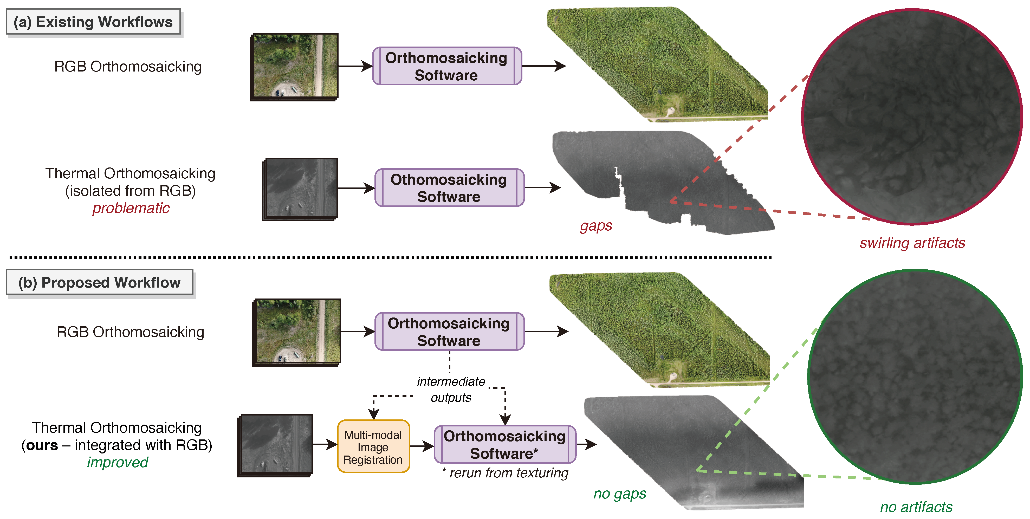
Figure 1. Comparison of (a) existing thermal orthomosaic generation workflows and (b) our proposed workflow that leverages intermediate outputs from RGB orthomosaic generation. Thermal-only processing workflows are prone to gaps and swirling artifacts (shown in red), which are tackled by our proposed workflow.
Remotesensing 15 02653 g001
Figure 2. Left: Location of Cynthia cutblock in Alberta, Canada. Red lines indicate provincial borders. Right: A close-up of the area including the village of Cynthia.
Remotesensing 15 02653 g002
Figure 3. Our integrated RGB–thermal orthomosaicking workflow. Example images of each type of data are also included, connected by dashed lines. Stage 3 is depicted in more detail in Figure 4.
Remotesensing 15 02653 g003
Figure 5. Internal mechanism of the Homography Module, which leverages the matrix exponential to compute the affine transformation matrix M using 6 basis matrices B and learnable scalar parameters v. The same 3 × 3 matrix C is used to update A at each of the 10 substeps, which are finally summed to yield M. The term eye(3) denotes the identity matrix of size 3 × 3.
Remotesensing 15 02653 g005
Figure 6. Graphical user interface (GUI) for our open-source orthomosaicking tool.
Remotesensing 15 02653 g006
Figure 7. Box (interquartile range, IQR) and whisker (within 1.5× IQR) plot showing mutual information (MI) of the 814 individual RGB–thermal image pairs using different co-registration techniques from the August 30 Cynthia flight data. NGF is normalized gradient fields [38], while ECC is enhanced correlation coefficient [28]. The white circles denote mean values.
Remotesensing 15 02653 g007
Figure 8. Visualization of orthomosaics generated from August 30 Cynthia cutblock data. (a) Georeferenced RGB orthomosaic. (b) Georeferenced thermal orthomosaic from unregistered images. (c) Georeferenced thermal orthomosaic from NGF-registered images. The improved quality of the orthomosaic in (c) is especially evident from the circular inset showing a straight path between the trees (similar to (a)) compared to the jagged path in (b).
Remotesensing 15 02653 g008
Figure 9. Checkerboard visualization of two undistorted RGB images interlaced with their corresponding thermal images (a) before and (b) after performing image co-registration with our proposed workflow. Colored squares correspond to the RGB images and grayscale ones to the thermal images.
Remotesensing 15 02653 g009
Figure 10. Visual and radiometric similarity between thermal images and the thermal orthomosaic. (a) A thermal image, (b) its corresponding patch in the thermal orthomosaic generated from our proposed workflow, and (c) temperature histograms for both in equally spaced bins of 0.1 °C.
Remotesensing 15 02653 g010
Figure 11. Visualization of downstream tree crown detection task performance for the August 30 Cynthia data. (a) Detected tree crowns from the RGB orthomosaic. The percentages represent the detection model’s confidence score for each RGB crown. (b) Corresponding patches extracted from the thermal orthomosaic at the same pixel locations as in (a).
Remotesensing 15 02653 g011
Table 1. Summary of Cynthia cutblock data for each flight date. Temperature and humidity values are taken from three weather stations closest to the cutblock and averaged.
20 Jul26 Jul9 Aug17 Aug30 Aug
Number of RGB–Thermal Image Pairs827828820825814
Average Air Temperature (°C)20.320.819.824.525.4
Average Relative Humidity (%)42.761.053.040.746.3
Table 2. Average MI of individual RGB and thermal images obtained using different design choices in our proposed workflow for five flights over the Cynthia cutblock. The best values are emboldened.
Design ChoiceJul 20Jul 26Aug 09Aug 17Aug 30Mean
Unregistered0.05390.04730.06950.05890.06580.0591
Manual0.24170.17810.26120.22470.20030.2212
ECC0.16580.21410.17420.20510.20790.1934
NGF0.29990.20030.31810.27150.30380.2787
Perspective0.29940.19950.31760.27070.30520.2785
Affine0.29990.20030.31810.27150.30380.2787
Single-resolution0.02390.03230.02710.02620.02470.0268
Multi-resolution0.29990.20030.31810.27150.30380.2787
Batch size = 10.04200.03960.06020.05060.04770.0480
Batch size = 40.14200.07590.10530.13430.10360.1122
Batch size = 160.30030.19660.31760.26720.30170.2767
Batch size = 320.29660.19820.31820.26790.29990.2762
Batch size = 640.29990.20030.31810.27150.30380.2787
Random sampling0.30000.19630.31770.26820.30230.2769
Systematic sampling0.29990.20030.31810.27150.30380.2787
Table 3. Average, minimum, and maximum observed values for each affine transformation matrix M component over all flights, obtained through NGF-based co-registration. The coefficient of variation (CoV) for each component is reported in the final column. M i , j denotes the value in the ith row and jth column. M 3 , 1 and M 3 , 1 are always 0 for affine transformation matrices and thus omitted.
ComponentAverageMinimumMaximumCoV (%)
M 1 , 1 1.014421.013801.0152000.05
M 1 , 2 0.006180.005790.0066004.45
M 1 , 3 0.025370.020750.03024012.19
M 2 , 1 −0.00861−0.01397−0.00599033.69
M 2 , 2 0.945460.944420.9467300.08
M 2 , 3 −0.06670−0.08146−0.04987016.40
M 3 , 3 1.042591.041531.0439700.09
Disclaimer/Publisher’s Note: The statements, opinions and data contained in all publications are solely those of the individual author(s) and contributor(s) and not of MDPI and/or the editor(s). MDPI and/or the editor(s) disclaim responsibility for any injury to people or property resulting from any ideas, methods, instructions or products referred to in the content.