Attention-Aware Spectral Difference Representation for Hyperspectral Anomaly Detection

Abstract

Hyperspectral Anomaly Detection (HAD) aims to detect the pixel or target whose spectral characteristics are significantly different from the surrounding pixels or targets. The effectiveness of reconstructing the background model is an essential element affecting the improvement of the HAD performance. This paper proposes a Hyperspectral Anomaly Detection method based on Attention-aware Spectral Difference Representation (HAD-ASDR) to reconstruct more accurate background models by using the generated noise distribution matchable to the background as input. The proposed HAD-ASDR mainly includes three modules: Attention-aware Spectral Difference Representation Module (ASDRM), Convolutional Auto-Encoder based Background Reconstruction Module (CAE-BRM) and Joint Spectrum Intensity and Angle based Anomaly Detection Module (JSIA-ADM). First, inspired by Generative Adversarial Network (GAN), ASDRM is proposed to generate a noise distribution that better matches the background by the attention mechanism and the different operation. Then, CAE-BRM is employed to reconstruct the accurate background using the generated noise distribution as input and the convolutional auto-encoder with skip connections. Finally, JSIA-ADM is presented to detect anomalies more accurately by calculating the reconstructed errors from both spectral intensity and angle perspectives. The proposed HAD-ASDR has been verified on five data sets and achieves better or comparable HAD results compared to six other comparison methods. The average AUC of HAD-ASDR on these five data sets is 0.9817 higher than that of the comparison methods, resulting in an improvement of 0.0253. The experimental results demonstrate its superior performance and stability.

1. Introduction

Hyperspectral imaging techniques aim to analyze a wide spectrum of light instead of only three basic colors (red, green, and blue). Hyperspectral images (HSI) generally contain hundreds or even several thousand bands to provide more information about each pixel, which can be utilized to distinguish targets and other objects from background clutter. This has led to its application in a variety of domains, including target classification [1], change detection [2] and anomaly detection [3].

Hyperspectral Anomaly Detection (HAD) is an important task in the HSI processing. The purpose of HAD is to identify pixels or regions whose spectral properties differ significantly from those of nearby pixels or the entire background map. The main difference between HAD and hyperspectral target detection is that HAD does not require a priori knowledge of the anomaly and the background’s scene. In the HSI, the pixels or objects whose spectral curve are significantly distinguished from the surrounding environment are defined as anomalies, and the remaining pixels or objects in the HSI are viewed as the background. HAD can be applied to environmental monitoring [4], defense reconnaissance [5] and mineral exploration [6] fields.

The existing HAD methods can be roughly classified into traditional HAD methods and deep learning based HAD methods [7,8]. Traditional HAD methods are mainly classified into statistical [9], representation based [10], and tensor decomposition based [11] methods. All these traditional HAD methods rely on manual features or shallow features learned by the statistical model, sparse representation, collaborative representation, matrix decomposition and so on. Hence, they cannot represent anomalies very well and distinguish anomalies from the background very well.

Since deep learning techniques have the ability to extract abstract, hierarchical and deep features that can represent anomalies or the background more accurately, many deep learning structures, such as Deep Belief Nets (DBN) [12], Auto-Encoder (AE) [13], Convolutional Neural Network (CNN) [14], Recursive Neural Network (RNN) [15], Long Short-Term Memory (LSTM) [16] and Generative Adversarial Network (GAN) [17], are applied to HAD tasks.

Since the types of anomalies vary with the different environmental scenes and the sizes of the anomalies are generally small in the HAD task, it is difficult to directly model anomalies, which is a challenge for improving the HAD performance. As a result, a larger number of traditional HAD methods and deep learning based HAD methods focus on identifying anomalies by constructing a background model. Therefore, the ability of the constructed background model to accurately represent the background is a significant factor affecting the HAD performance. However, in most real-world scenarios, the background land cover types are various and complex, which can lead to inaccuracies in background modeling for HAD algorithms.

Our goal is to consider various and complex land cover types when generating the background, in order to construct a more accurate background model and thereby improve the accuracy of HAD. Therefore, a HAD method based on Attention-aware Spectral Difference Representation (HAD-ASDR) is proposed, which guides a more accurate background reconstruction by generating the noise distribution that better matches the background. The proposed HAD-ASDR contains three modules: Attention-aware Spectral Difference Representation Module (ASDRM), Convolutional Auto-Encoder based Background Reconstruction Module (CAE-BRM), and Joint Spectrum Intensity and Angle based Anomaly Detection Module (JSIA-ADM). With the use of spectral channel and spatial attention mechanisms, as well as the corresponding difference operations between the input images and the learned features, ASDRM seeks to generate a noise distribution that more accurately represents the background, which contains various and complex land cover types. CAE-BRM uses the above-mentioned generated noise as input to reconstruct the more accurate background. JSIA-ADM aims to better detect anomalous pixels by measuring the reconstruction errors from both the spectral intensity and angle perspectives. Experiments are conducted on five real hyperspectral data sets to prove the efficacy of the proposed HAD-ASDR method. It achieves superior or equivalent HAD results when compared with six other methods.

The main contributions of our study can be summarized as follows:

(1)

An attention-aware spectral difference representation module is proposed to generate a noise distribution that better matches the background by employing the attention mechanism and spectral difference strategy, which can guide the construction of a more accurate background model in situations where the types of land covers are diverse and complex.

(2)

A compound loss function is designed to better detect anomalies, which simultaneously calculates the reconstruction errors between the original input image and the reconstructed image from both the spectrum intensity and angle perspectives.

(3)

The proposed HAD-ASDR method is verified on five hyperspectral data sets and achieves better or comparable HAD performance than the comparison HAD methods.

2. Related Work

2.1. Hyperspectral Anomaly Detection Method

HAD is generally defined as an unsupervised task without requiring prior knowledge of the background or anomalies [18]. HAD methods can be categorized into two groups: traditional HAD methods and deep learning based HAD methods [19].

Statistical based, representation based, and tensor decomposition based methods form the primary categories for traditional HAD methods [20,21]. Assuming that the background makes up the majority of the images for the HAD task, a Gaussian distribution is utilized by numerous methods to model the background, which provides the possibility to statistically separate anomalies from the background. The RX method [9], proposed by Reed-Xiaoli, is one of the classical methods based on statistics, and can be viewed as Global RX (GRX). The Local RX (LRX) methods improve the RX method from the local perspective by estimating the background statistics using the local sliding double windows for HAD. There are other RX based HAD methods such as Kernel RX [22] for improving the HAD performance. The HSIs acquired in real scenes do not always obey the Gaussian distribution [23], which will make the detection outcomes of the RX based methods not always unsatisfactory. The representation based HAD methods make the assumption that certain coefficients in a specific constructed dictionary can collaboratively represent the background and anomalous pixels [24]. Li et al. [25] proposed a HAD method that incorporates background joint sparse representation (BJSR) and an adaptive subspace based detector. The approach assumes that neighboring pixels belonging to the same subspace can accurately represent background pixels, whereas anomalous pixels cannot. Li et al. [26] presented a HAD technique (LTDD) that employs low-rank tensor decomposition to decompose the HSI data cube into a 3D tensor. The background is modeled as a low-rank matrix, while anomalies are represented by a sparse matrix. To detect anomalies, an unmixing method based on LTDD is applied to the decomposed tensor, resulting in the effective anomaly detection. Kang et al. [27] introduced a novel hyperspectral anomaly detection approach that employs attribute filtering for initial detection and edge-preserving filtering for post-processing to improve the HAD performance. The majority of the above-mentioned traditional HAD methods might face difficulties in accurately modeling backgrounds with a variety of intricate features, which can result in false alarms or undetected anomalies.

Deep learning based HAD methods can be classified according to the network structure used. The network structures such as CNN, AE, GAN, DBN, LSTM are applied to HAD tasks. Fu et al. [28] presented a HAD method based on a Plug-and-play regularized denoising CNN, which used a denoised CNN network introduced into the background dictionary construction to address the problem of requiring a priori representation coefficients, and finally achieved the anomaly detection map from the clustering results. Bati et al. [29] utlized the AE structure to extract the overcomplete representation of hyperspectral images through the encoding and decoding operations, and anomalies are identified by computing reconstruction errors in the detection stage. Xie et al. [30] designed a semi-supervised HAD method based on the AE network and the adversarial learning strategy, which was trained to estimate the background using high probability background samples obtained by clustering as labels, and captured the background by the joint adversarial reconstruction loss. Chang et al. [31] presented a sparse AE network, which used pixels in concentric double-window as the network input to make the learned features more representative, and the residuals of the reconstruction errors were viewed as the anomaly detection results. Jiang et al. [32] designed a HAD method based on GAN, which combined the discriminators of GAN and AE to learn the normal distribution of the background in the potential feature layer, and finally generated the anomaly detection map using a joint space and distance detector. Ma et al. [18] presented a HAD method based on DBN. It used DBN to extract the discriminatory characteristics of hyperspectral images and adaptive weights to minimize the impact of anomalies on the reconstructed background, then utlized the Euclidean distance to separate anomalies from the background. Zhu et al. [33] presented a HAD method based on LSTM and AE, which utilized the internal control machine in LSTM to fit the spectral continuity of HSI data in adjacent bands by adjusting the context propagation to make the reconstructed background more accurate, used principal component analysis to downscale the reconstructed image to reduce the anomalous information, and finally used the Mahalanobis distance to measure the anomalies. The deep learning based HAD methods mentioned above have achieved promising results. However, they did not pay sufficient attention to the impact of feature diversity and complexity on the accuracy of background model construction, which will affect the HAD performance.

2.2. Convolutional Auto-Encoder

Auto-Encoder (AE) is a type of unsupervised deep learning network. It aims to convert input data to output data with minimal loss, which is usually used for compressing data, image denoising [34]. Convolutional Auto-Encoder (CAE) [35] introduces the convolutional operations to AE to improve spatial feature extraction and learning ability, which is applied to the HSI processing, such as hyperspectral classification [36], hyperspectral anomaly detection and target detection [37].

In the field of hyperspectral classification, Zhao et al. [38] designed a multiscale convolution autoencoder to extract global deep features, which used a logistic regression classifier to classify the learned deep features. In the hyperspectral anomaly detection, Hosseiny and Shah-Hosseini [39] designed a stacked auto-encoder to extract deep and nonlinear features using a 1D AE and a 2D AE, and then performed the anomaly detection based on the reconstruction error of the target pixels in each segmented map. Shi et al. [40] designed a 3D residual CAE for target detection, which extracts features at different spatial scales and fuses them to separate the target from the background using distance-constrained errors. This method achieves accurate and robust segmentation results by combining information from multiple scales.

2.3. Attention Mechanism

The attention mechanism in the computer vision field refers to selectively concentrating on one or a few objects in the images while ignoring others. The attention mechanism is a technique used in deep learning models that enables the model to focus on important elements of the input data by assigning weights to different parts of the input. By dynamically adjusting these weights during training, the model can effectively filter out irrelevant information and concentrate on the most salient features, leading to the improved accuracy and efficiency. Hence, the attention mechanism is widely applied to image generation [41], classification, target recognition and other tasks.

In the area of image generation, Chen et al. [42] introduced the attention mechanism into GAN by guiding the network attention to the relevant regions of audiovisual signals and designing a dynamically tunable pixel loss function with the attention mechanism to generate more robust images. In the field of classification, Cai and Wei [43] designed an algorithm based on the graph convolution network and the cross-attention mechanism, which utilizes the joint horizontal and vertical weight assignment to obtain features of an image. Then, the low-dimensional features obtained by the principal component analysis are combined to complete the image prediction. In the target detection field, Ju et al. [44] presented an improved the YOLO V3 and DSSD network for target detection, which used global and spatial attention mechanisms to learn features at different scales for adaptive fusion, and then improved the detection performance by a constructed multi-scale target detector.

3. Method

The proposed HAD-ASDR is shown in Figure 1, which is mainly composed of three modules: ASDRM, CAE-BRM and JSIA-ADM. ASDRM extracts more discriminative features of anomalies by the spatial and spectral channel attention blocks, and then uses the auto-encoder and the difference operations to generate the noise distribution that better matches the background. CAE-BRM uses the generated noise distribution learned by ASDRM as input and then employs the convolutional auto-encoder with skip connections to reconstruct the background more accurately. JSIA-ADM utilizes the reconstruction errors calculated between the input hyperspectral image and the background reconstructed by CAE-BRM from both the spectral intensity and angle perspectives in order to achieve a more accurate anomaly detection map.

3.1. Attention-Aware Spectral Difference Representation Module

Anomalies in the hyperspectral images generally are rare and smaller than the background, which have a low probability of occurring in the hyperspectral images. Moreover, since hyperspectral images contain a lot of noises, it is difficult to detect anomalies directly from hyperspectral images. It is a reasonable method to generate the anomaly detection map by constructing a background model and comparing it with the input hyperspectral image. Hence, the accuracy of the reconstructed background model is one of the important factors influencing the HAD performance. Inspired by the GAN that uses the noise as input and generates an image as output, we try to reconstruct the background image from the noise. Since the noise distributions of different backgrounds are different, ASDRM in the proposed HAD-ASDR is presented to generate a noise distribution that better matches the background to make the reconstructed background more accurate. ASDRM contains a spectral channel attention block, a spatial attention block, an auto-encoder block and difference operations.

The spectral channel attention block, the spatial attention block, and the auto-encoder block are denoted as $B_{SCA}$, $B_{SA}$ and $B_{AE}$, respectively. The structure of $B_{SCA}$, $B_{SA}$ and $B_{AE}$ is shown in

Table 1. Structure of the blocks in the Attention-aware Spectral Difference Representation Module (ASDRM).

Block	Layer	Input	Kernel Size	Stride Size	Output
Spectral chanel attention	Avg_pool	(C,H,W)	-	-	(C,1,1)
	Conv2d	(1,C,1,1)	(1,1)	(1,1)	(1,C,1,1)
	Conv2d	(1,C,1,1)	(1,1)	(1,1)	(1,C,1,1)
	Max_pool	(1,C,1,1)	-	-	(C,1,1)
	Conv2d	(1,C,1,1)	(1,1)	(1,1)	(1,C,1,1)
	Conv2d	(1,C,1,1)	(1,1)	(1,1)	(1,C,1,1)
Spatial attention	Concat	2 × (1,1,H,W)	-	-	(1,2,H,W)
	Conv2d	(1,2,H,W)	(7,7)	(1,1)	(1,1,H,W)
Auto-encoder	Conv2d	(1,C,H,W)	(3,3)	(1,1)	(1,128,H,W)
	Conv2d	(1,128,H,W)	(3,3)	(1,1)	(1,64,H,W)
	Conv2d	(1,64,H,W)	(3,3)	(1,1)	(1,32,H,W)
	ConvTranspose2d	(1,32,H,W)	(3,3)	(1,1)	(1,64,H,W)
	ConvTranspose2d	(1,64,H,W)	(3,3)	(1,1)	(1,128,H,W)
	ConvTranspose2d	(1,128,H,W)	(3,3)	(1,1)	(1,C,H,W)

. The structure of $B_{SCA}$ includes an average pooling layer (Avg_pool), a maximum pooling layer (Max_pool) and four convolutional layers (Conv2d). The kernel size of the four Conv2d is (1,1) with a stride of (1,1). The extended dimensional operation after the Avg_pool and the Max_pool layers is added to ensure that the upper and lower layers are the same size. $B_{SA}$ compute the mean and maximum values of the features extracted from $B_{SCA}$ at first, and then the mean and maximum values are concatenated and fed to a Conv2d with kernel size of (1,1) and a stride of (1,1). $B_{AE}$ contains of three Conv2d and three deconvolution layers (ConvTranspose2d). The kernel size of three Conv2ds and ConvTranspose2ds are (3,3) with a stride size of (1,1). All three blocks utilize the sigmoid function as the nonlinear activation function. ASDRM is trained by the loss function MSE for 50 epochs to obtain the optimal model.

It is noteworthy that ASDRM employs a spectral channel and spatial attention mechanism that aims to explore the targets that are different from others in the image. Hyperspectral anomaly detection seeks to detect targets whose spectrum is much different from that of surrounding pixels. Therefore, the purpose of HAD is very close to that of the spectral channel and spatial attention mechanism. The spectral channel attention block and the spatial attention block in the proposed ASDRM are utilized to search for anomalies. The noise of the background is obtained by two different operations.

The process of ASDRM is as follows: firstly, the hyperspectral image with the size of $C\times H\times W$ (C, H, W represents depth, height and width) as input, denoted as X, is fed to $B_{SCA}$ block to extract features by considering the spectral channel attention mechanism, denoted as $F_{SCA}$. Secondly, $F_{SCA}$ is fed to $B_{SA}$ block to obtain features with taking both the channel and spatial attention into account, denoted as $F_{SA}$. Thirdly, the initial background $F_{IB}$ is achieved by subtracting $F_{SA}$ from the original input X. The difference operation is utilized as shown in Equation (1). Fourthly, the initial background $F_{IB}$ is fed to the auto-encoder block $B_{AE}$ to obtain the reconstructed background $F_{RB}$. Finally, the noise of the background $N_B$ can be calculated by Equation (2), which is obtained by subtracting $F_{RB}$ from $F_{IB}$.

$$F_{IB}=X-F_{SA}$$

(1)

$$N_B=F_{IB}-F_{RB}$$

(2)

3.2. Convolutional Auto-Encoder Based Background Reconstruction Module

Since CAE is an unsupervised learning network that does not need any label information to train, it matches the hyperspectral anomaly detection tasks that require no prior information. Hence, CAE is used as the backbone structure to reconstruct the background. Moreover, the skip connections are added to CAE to enhance the discriminative ability of learned features by considering intermediate information to make up for the information loss during the reconstruction process.

The background noise generated by ASDRM is used as the input to CAE-BRM. CAE-BRM contains two blocks: the encoder and decoder. The encoder includes 15 convolutional layers, all of which have 128 neurons. The first and second convolutional layers have the kernel sizes of $1\times 1$ and $3\times 3$, and the stride sizes of 1 and 2, respectively. The middle layers are a combination of four three-layer convolutions with the kernel size of $3\times 3$, $1\times 1$ and $3\times 3$, the stride sizes of 1, 1 and 2, respectively. The last layer is a convolutional layer with the kernel size of $3\times 3$ and the stride size of 1.

The decoder consists of 11 convolutional layers and 5 up-sampling operations, where the number of neurons in each of the convolutional layers is 128 and the up-sampling operation is a nearest-neighbor interpolation with a scale of 2. The decoder starts with an up-sampling operation, followed by four combinations of a convolution with the kernel size of $3\times 3$ and the stride size of 1, a convolution with the kernel size of $1\times 1$ and the stride size of 1, and an up-sampling operation. The last three convolutional layers have kernel sizes of $3\times 3$, $1\times 1$, $3\times 3$ and the stride sizes of 1, 3, 1, respectively. The skip connection has the ability to compensate for the pixel-level feature information lost by downsampling in the encoding stage. Hence, the outputs of the 1st, 4th, 7th, 10th and 13th convolutional layers of the encoder are skip-connected to the feature maps obtained from the up-sampling operation in the decoder in turn. For example, the output of the 13th convolutional layer of the encoder and the feature map obtained from the first up-sampling operation of the decoder are fed into the first convolutional layer of the decoder. Some important information in the encoder can be retained by adding the skip connections, which will achieve a more accurate background. The output of CAE-BRM is the reconstructed background, denoted as $X_R$.

CAE-BRM is trained by a compound loss function that calculates the similarity based on both the spectral intensity and angle. The total loss function of CAE-BRM $L_{all}$ contains two terms: $L_1$ and $L_2$. $L_1$ represents the spectral intensity loss. $L_2$ means the spectral angle loss. $L_{all}$ of CAE-BRM is defined as follows:

$$L_{all}=L_1+\alpha L_2$$

(3)

where $\alpha$ is the penalty parameter for the spectral angle loss $L_2$ that aims to adjust the contribution of $L_2$ to $L_{all}$. The formulas of $L_1$ and $L_2$ can be defined as follows:

$$L_1(X,X_R)=\frac{1}{n}\sum _{i=1}^n{∥X_i-X_{R_i}∥}_1$$

(4)

$$L_2(X,X_R)=\frac{1}{n}\sum _{i=1}^n{cos}^{-1}(\frac{{X_{R_i}}^T{X_i}^{*}}{\left(∥X_{R_i}∥\right)\left(∥{X_i}^{*}∥\right)})$$

(5)

where n denotes the number of pixels in the input hyperspectral image. $X_i$ and $X_{R_i}$ represent the ith pixel of the input hyperspectral image X and the output of CAE-BRM $X_R$, $i\in [1,n]$.

3.3. Joint Spectrum Intensity and Angle Based Anomaly Detection Module

Assuming anomalies in hyperspectral images are rare and have a low possibility of occurrences, the majority of input samples of CAE-BRM belong to the background. Hence, CAE-BRM has the ability to learn background patterns. When a background pixel is fed to the learned model, it satisfies the background patter with a small reconstruction error. On the contrary, when an anomalous pixel is fed to the learned model, it does not satisfy the background pattern with a larger reconstruction error. Hence, the reconstruction error can be utilized to detect anomalies. However, if the reconstructed error is calculated only from the spectral intensity perspective, the important spectral curves of land covers in hyperspectral images are not considered, which has proved to be effective for detecting targets in hyperspectral images. Moreover, the total loss function of CAE-BRM $L_{all}$ shown in Equation (3) includes the spectral intensity loss function and the spectral angle loss function. Hence, in order to fully utilize the spectral information of hyperspectral images, JSIA-ADM is proposed in the HDM-ASDR to detect anomalies by calculating the reconstructed errors based on joint spectral intensity and angle.

The reconstructed error of the ith pixel based on joint spectral intensity and angle, denoted as $RErro{r}^i$, can be calculated as follows:

$$RErro{r}^i=RErro{r}_{Intensity}^i+\alpha RErro{r}_{Angle}^i$$

(6)

where $RErro{r}^i$ represents the total reconstructed error of the ith pixel, $i\in [1,n]$. $RErro{r}_{Intensity}^i$ means the reconstructed error of the ith pixel computed by the spectral intensity. $RErro{r}_{Angle}^i$ denotes the reconstructed error of the ith pixel computed by the spectral angel. $\alpha$ is the penalty parameter for $RErro{r}_{Angle}^i$ that aims to adjust the contribution of $RErro{r}_{Angle}^i$ to the total reconstructed error of the ith pixel $RErro{r}^i$.

The $RErro{r}_{Intensity}^i$ and the $RErro{r}_{Angle}^i$ can be computed by the following formulas:

$$RErro{r}_{Intensity}^i(X_i,{\widehat{X}}_i)={∥X_i-{\widehat{X}}_i∥}_1$$

(7)

$$RErro{r}_{Angle}^i(X_i,{\widehat{X}}_i)={cos}^{-1}(\frac{{{\widehat{X}}_i}^T{X_i}^{*}}{\left(∥{\widehat{X}}_i∥\right)\left(∥{X_i}^{*}∥\right)})$$

(8)

where $X_i$ is the ith pixel in the input hyperspectral image. ${\widehat{X}}_i$ represents the ith pixel in the reconstructed image, $i\in [1,n]$.

3.4. The Process of HAD-ASDR

In the training stage, the optimizing process is composed of ASDRM and CAE-BRM. Firstly, the hyperspectral image is fed to the $B_{SCA}$ block to obtain features $F_{SCA}$. Secondly, the learned $F_{SCA}$ is fed to $B_{SA}$ block to obtain features $F_{SA}$. Thirdly, the initial background $F_{IB}$ is calculated according to Equation (1). Fourthly, $F_{IB}$ is fed to $B_{AE}$ to generate the reconstruction background $F_{RB}$. Fifthly, the optimal ASDRM is obtained through updating all the parameters by utilizing Adam optimizer to minimize MSELoss. Sixthly, the noise of the background $N_B$ is calculated according to Equation (2). Seventhly, $N_B$ is fed to CAE-BRM to obtain the reconstructed background $X_R$. Eighthly, the overall loss $L_{all}$ is computed according to Equation (3). Ninthly, the optimal CAE-BRM is obtained through updating all the parameters by utilizing Adam optimizer to minimize $L_{all}$ in Equation (3). Finally, the final reconstructed image $\widehat{X}$ is obtained by feeding the input hyperspectral image to the learned optimal ASDRM and CAE-BRM, and the anomaly detection map is achieved by calculating reconstruction errors between X and $\widehat{X}$ using Equation (6). The process of HAD-ASDR is shown in Algorithm 1.

Algorithm 1 The process of HAD-ASDR.

Input:

The hyperspectral images X.

Initialization:

1. Adam optimizer is used in the ASDR model, and the learning rate is set to   1 × 10$-3$.

The loss function is MSELoss, and the number of epochs is set to 50.

2. The Adam optimizer is used in the CAE-BRM, the learning rate is set to 1 × 10$-2$,             and the loss function is used in Equation (3).

Step:

1. Feed X into the $B_{SCA}$ block to obtain $F_{SCA}$.

2. Feed the learned $F_{SCA}$ to the $B_{SA}$ block to obtain $F_{SA}$.

3. The initial background $F_{IB}$ is calculated by Equation (1).

4. Feed $F_{IB}$ to $B_{AE}$ to generate the reconstructed background $F_{RB}$.

5. Update all the parameters by utilizing Adam optimizer to minimize MSELoss.

Until: achieve the optimal ASDR model after a fixed number of epochs.

6. Calculate the noise of the background $N_B$ by Equation (2).

7. Feed $N_B$ to CAE-BRM to obtain the reconstructed background $X_R$.

8. Compute the overall loss $L_{all}$ according to Equation (3).

9. Update all the parameters by minimizing $L_{all}$ utilizing Adam optimizer.

Until: achieve the optimal CAE-BRM model after a fixed number of epochs.

10. The anomaly detection map is achieved by calculating reconstruction errors             between X and $\widehat{X}$ obtained from the optimal ASDR and CAE-BRM by Equation (6).

Output:

1. The anomaly detection map.

2. Area Under Curve (AUC) values.

4. Experiments and Analysis

4.1. Data Sets

To validate the efficacy of the proposed HDM-ASDR method, we carried out experiments on five real hyperspectral data sets that will be described in the following.

(1)

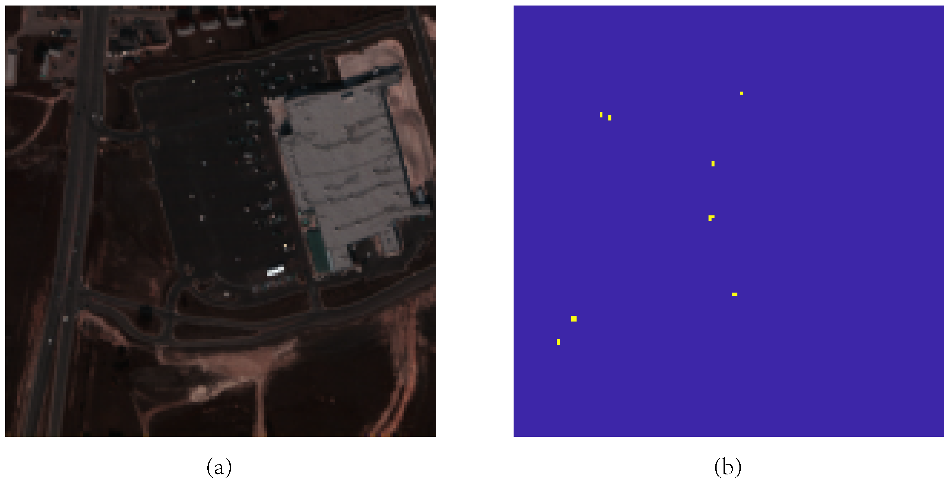
AVIRIS Airplane Data: The AVIRIS sensor is utilized to shoot the specific area of San Diego, CA, USA to acquire the AVIRIS airplane data. The AVIRIS airplane data has a spatial resolution of 20 m and a spectral resolution of 10 nm, whose spectral wavelengths span from 370 to 2510 nm. The AVIRIS airplane image has the spatial size of $100\times 100$ and 224 spectral bands. A total of 189 spectral bands are retained because of removing the bad or noise bands. In the hyperspectral image, three airplanes are classified as anomalies. The visualization of the AVIRIS airplane data and its corresponding ground truth are shown in Figure 2.

(2)

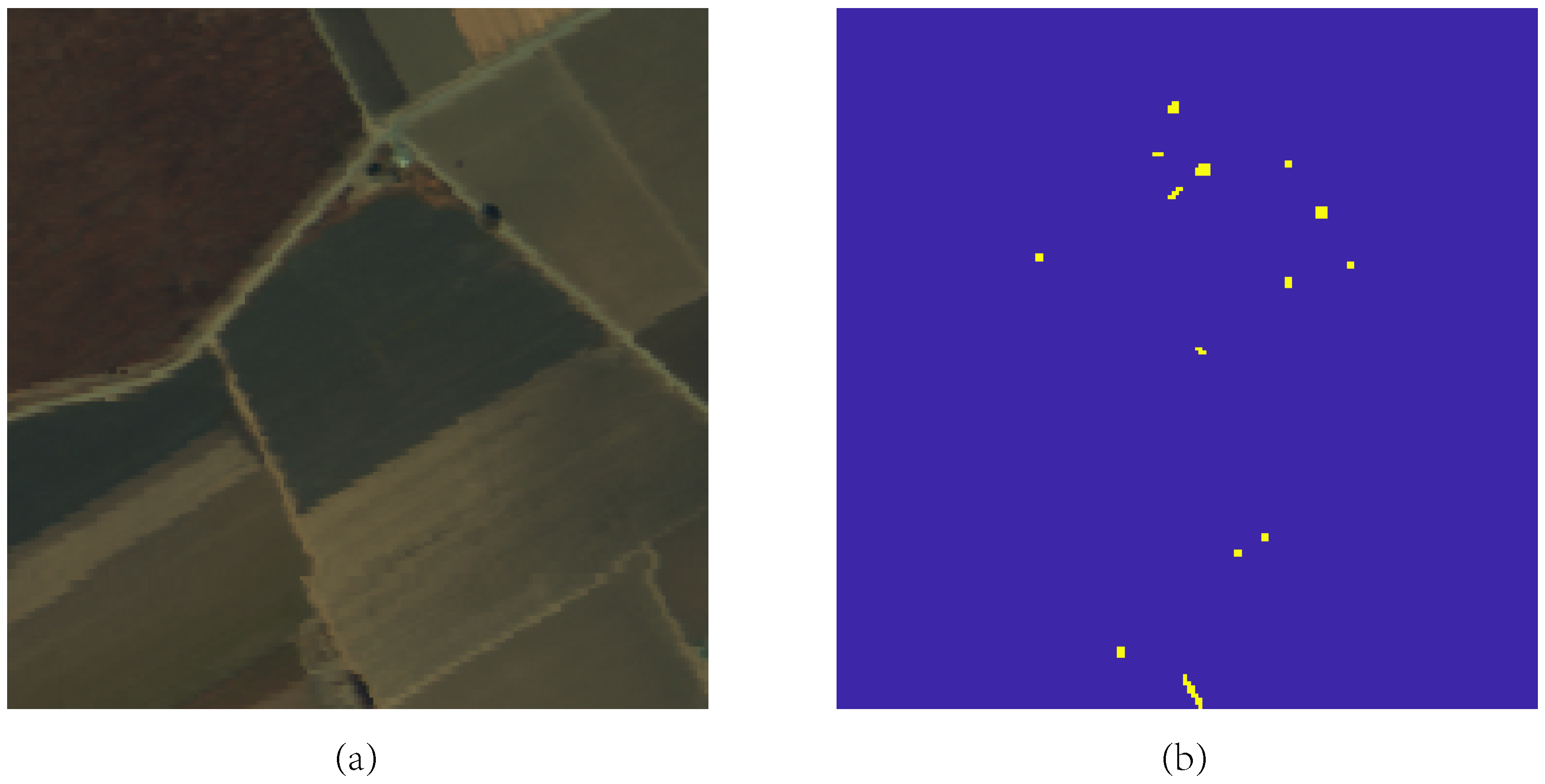
HYDICE Urban Data: The HYDICE airborne sensor is employed to collect HYDICE urban data. The HYDICE urban image has $150\times 150$ pixels in the spatial dimension and includes 210 spectral bands, with wavelengths ranging between 400 and 2500 nm. 162 valid spectral bands have remained after removing bad bands such as low-SNR and water absorbing bands. The cars and roofs in these data are considered as anomalies. The HYDICE urban data and its corresponding ground truth are illustrated in Figure 3.

(3)

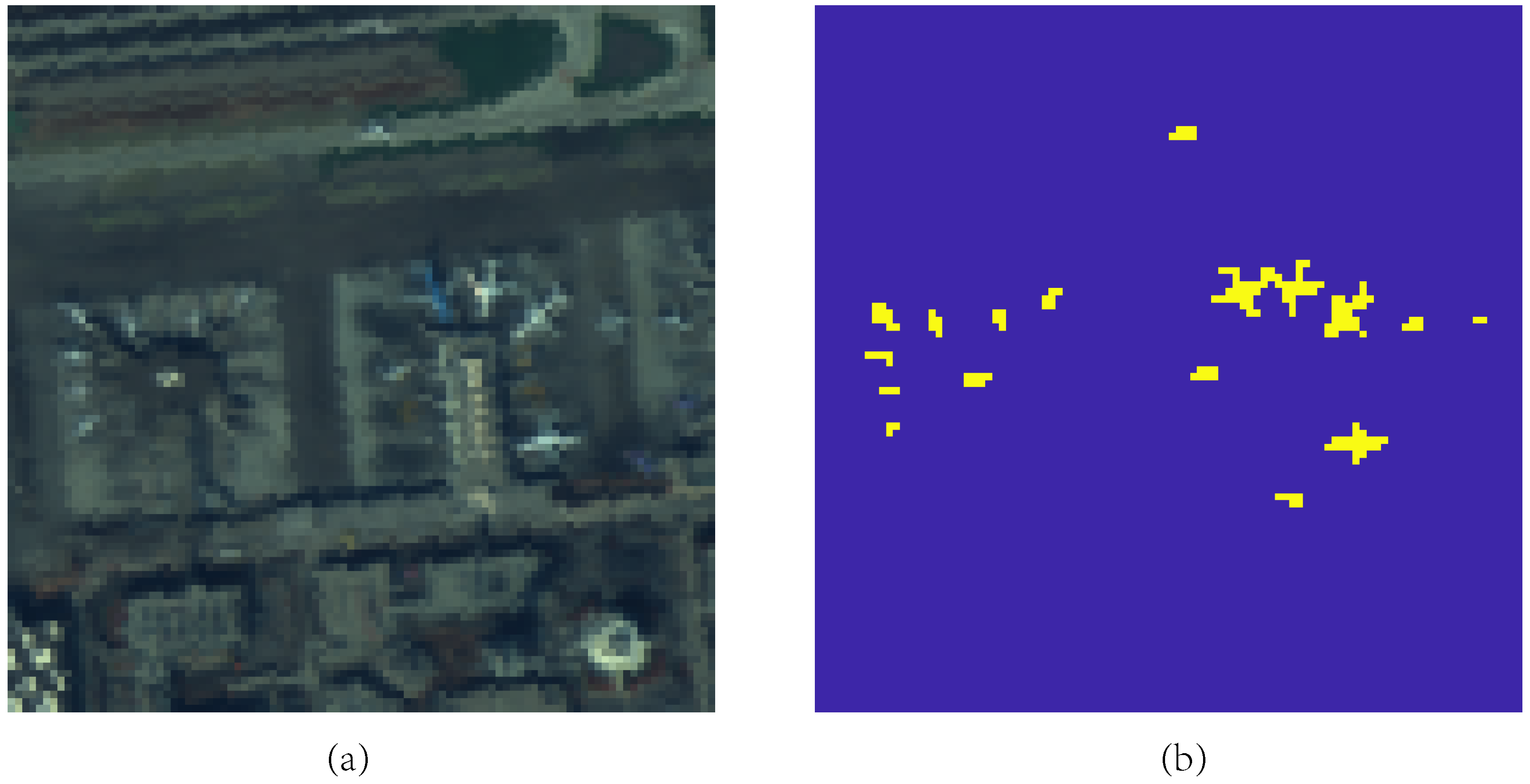
Salinas Scene Data: The AVIRIS sensor is utilized to shoot the Salinas valley of California, USA to acquire the Salinas scene data. The Salinas scene image has $180\times 180$ pixels in the spatial dimension and includes 224 spectral bands. Vegetables, vineyard fields, and bare soils are considered as anomalies in the Salinas scene. Figure 4 shows the Salinas scene data and their corresponding ground truth.

(4)

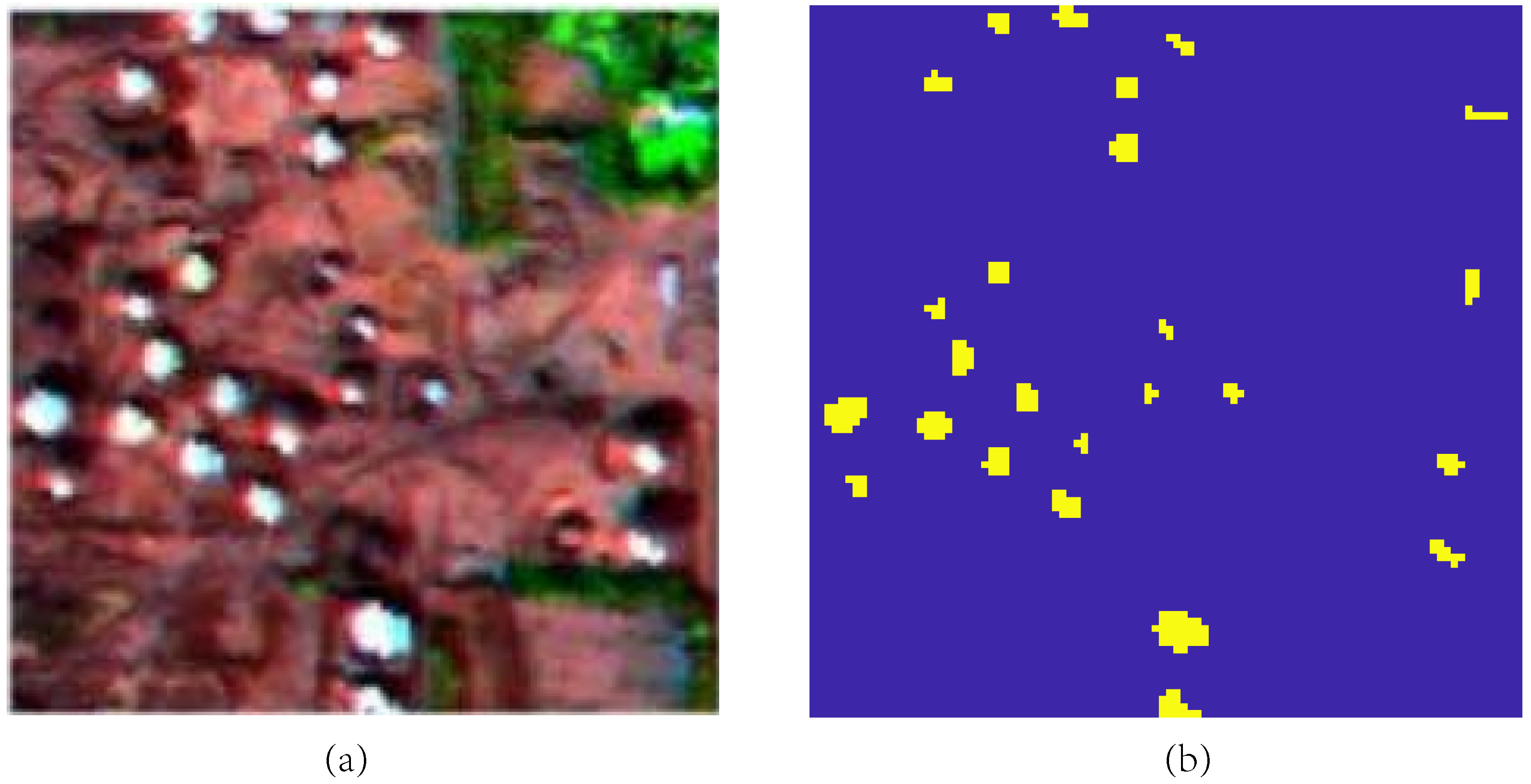
Abu-airport-3 Data: The AVIRIS sensor is utilized to collect Abu-airport-3 Data, which represents the airport in Los Angeles, USA. The Abu-airport-3 image consists of a spatial dimension of $100\times 100$ pixels and includes 205 spectral bands after removing bad bands. Airplanes in these data are considered anomalies. Figure 5 illustrates the Abu-airport-3 data and their corresponding ground truth.

(5)

Abu-urban-4 Data: The AVIRIS sensor is employed to capture data from the urban area in Los Angeles, USA, resulting in the Abu-urban-4 data. These data are collected using the same equipment as the Abu-airport-3 data. It has the spatial size of $100\times 100$ and 205 spectral bands after eliminating the bad or noise bands. Houses in these data are considered anomalies. Figure 6 displays the Abu-urban-4 data and their corresponding ground truth.

4.2. Evaluation Criteria

In order to fully evaluate the performance of the proposed HDM-ASDR method, we performed the qualitative and quantitative analysis using Receiver Operating Characteristic curves (ROC) and Area Under Curve (AUC) values.The ROC curve is a graph that illustrates how changing the discrimination threshold of a binary classifier affects its ability to correctly classify targets. It shows the relationship between the True Positive Rate (TPR) and False Positive Rate (FPR), with TPR plotted along the Y-axis and FPR plotted along the X-axis for different threshold values. By analyzing the ROC curve, we can determine the optimal threshold for our classifier based on the trade-off between sensitivity and specificity. The FPR and TPR are defined as

$$TPR=\frac{TP}{P}$$

(9)

$$FPR=\frac{FP}{N}$$

(10)

where $TP$ means that the sample is classified to be positive and the label is positive. P represents all samples with positive labels, $FP$ means the sample is classified to be positive but the label is negative, and N indicates all samples with negative labels. The AUC is a valuable metric for evaluating binary classifiers. It measures the area under the ROC curve and provides a standardized numerical measure of classification accuracy. When the AUC value is much closer to 1, the anomaly detection performance is better.

4.3. Training Parameters

The hyper-parameters in the experimental process of this method are described in this section. The proposed HAD-ASDR is implemented by Pytorch. The comparison and ablation experiments are run on a PC with an Intel(R) Core(TM) i7-7700HQ CPU, 2.80 GHz and the Windows 10 operating system.

The ASDR and the CAE-BRM module are trained separately. The ASDR model’s training epoch is set to 50. The batch size is 1. MSELoss is used as the loss function and the Adam optimizer are employed with the learning rate of $0.001$ to train ASDR. The CAE-BRM model’s training epoch is set to 600. The Adam optimizer is utlized with the learning rate of $0.01$. The loss function in Equation (3) is employed to train CAE-BRM, where $\alpha$ is $0.0001$.

4.4. Comparison with State-of-the-Arts

Six other methods are used to compare with the proposed HAD-ASDR to validate its effectiveness on five hyperspectral data sets. The comparison methods are listed as follows:

(1)

Local RX (LRX) [45] uses the strategy of the double sliding window for estimating local background statistics. It has the ability to identify anomalies by computing the Mahalanobis distance between a pixel under consideration and its surrounding pixels.

(2)

The Background Joint Sparse Representation (BJSR) [25] based method makes the assumption that each pixel can be represented by the constructed background dictionary and a specific coefficient, and employs the reconstructed errors to identify anomalies with large reconstructed errors.

(3)

Manifold Constrained AutoEncoder Network (MC-AEN) [46] based method extracts latent features by the auto-encoders with constraints by the manifold structure, and calculates the global and local reconstructed errors to detect anomalies.

(4)

The Autonomous Hyperspectral Anomaly Detection Network (Auto-AD) [47] method designs a fully convolutional auto-encoder architecture, which incorporates skip connections to reconstruct the background. An adaptive-weighted loss function is utilized to reduce the influence of potential anomalous pixels with large reconstruction errors in order to distinguish anomalies effectively.

(5)

DeCNN-AD algorithm [28] uses the clustering strategy to construct a new dictionary and incorporates a flexible denoiser as a prior for the representation coefficients in the dictionary to enhance the accuracy of HAD.

(6)

The LRSNCR algorithm [48] is a non-convex regularized approximation technique that builds on the improved RPCA for HAD. LRSNCR improves the discriminative ability between anomalies and the background significantly through the use of non-convex regularization.

The detection results of the comparison methods LRX and BJSR depend on the window size. The window sizes of LRX and BJSR are set to $W_{out}$ = $15\times 15$, $W_{in}$ = $3\times 3$ for five real data sets in our experiment.

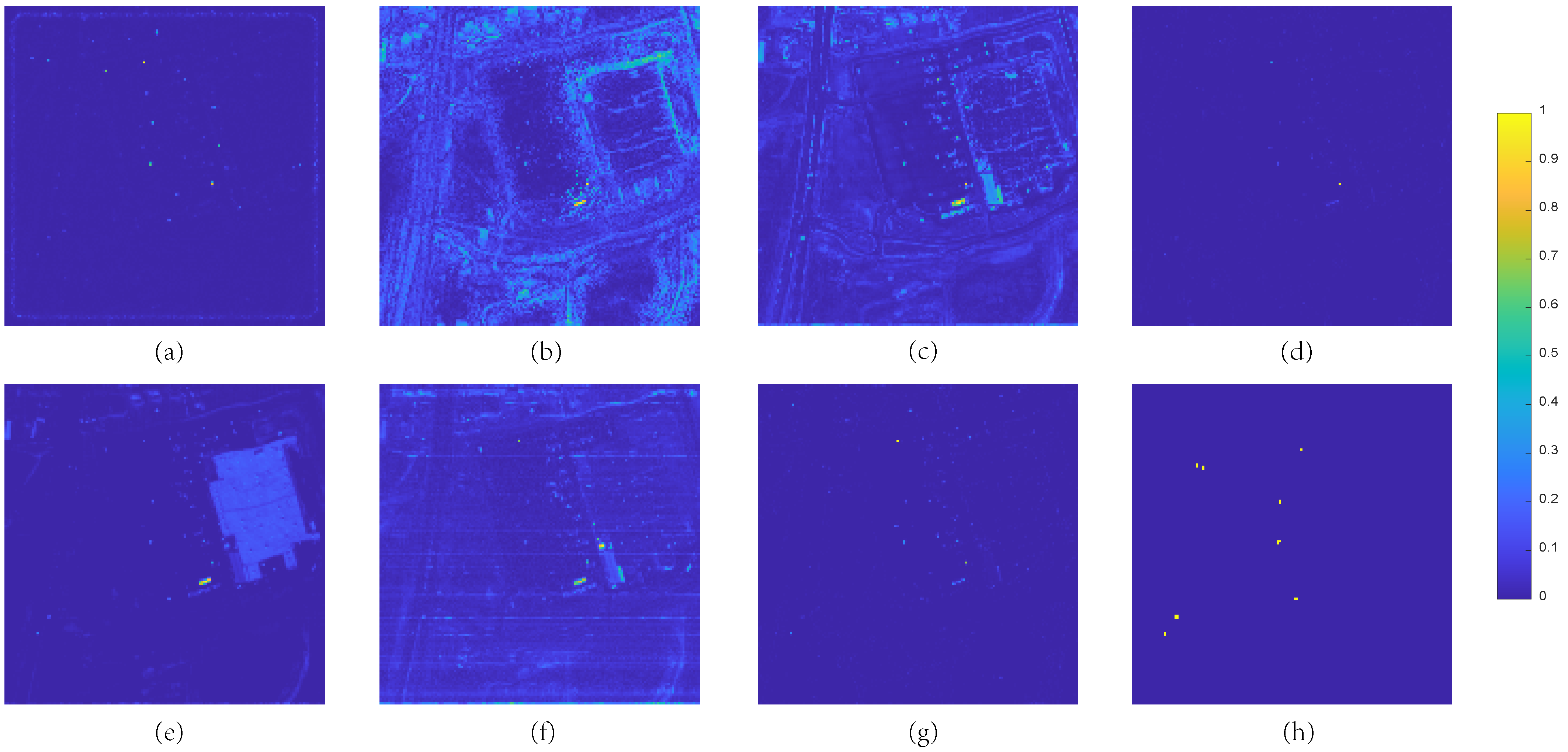
Figure 7 illustrates the visualized display of anomaly detection results on the AVIRIS airplane data set. Although BJSR and MC-AEN have a better detection ability for three airplanes, they have a relatively high false detection rate that incorrectly identifies many background pixels as anomalies. On the contrary, LRX has a relatively high miss detection rate that detects many anomalies as the background by mistake. Auto-AD fails to detect most anomalies. Although DeCNNAD, LRSNCR and the proposed HAD-ASDR can detect all the anomalies, DeCNNAD and LRSNCR incorrectly detect many background pixels in the upper-right of the image as anomalies with a high false detection rate. Compared with DeCNNAD and LRSNCR, the proposed HAD-ASDR has a lower false detection rate, especially in the upper-right of the image. It is obvious that the reconstructed background errors generated by HAD-ASDR are very small and close to 0. This is because the proposed HAD-ASDR makes the reconstructed background more accurate by considering the different noise distributions in different backgrounds.

The results of the anomaly detection analysis on the HYDICE urban data set are visualized in Figure 8. BJSR, MC-AEN and LRSNCR have higher false detection rates compared with the proposed HAD-ASDR, and some background pixels are incorrectly identified as anomalies. Although LRX, Auto-AD, DeCNNAD, and the proposed HAD-ASDR can separate anomalies from the background, LRX, Auto-AD and DeCNNAD have relatively higher miss detection rates. It is obvious that Auto-AD does not respond to anomalies significantly. Since the size of the anomalies in these data is relatively small, the proposed HAD-ASDR is more suitable for small anomalies because it calculates the reconstruction errors from both the spectral intensity and angle perspectives. Hence, the proposed HAD-ASDR achieves the best anomaly detection performance.

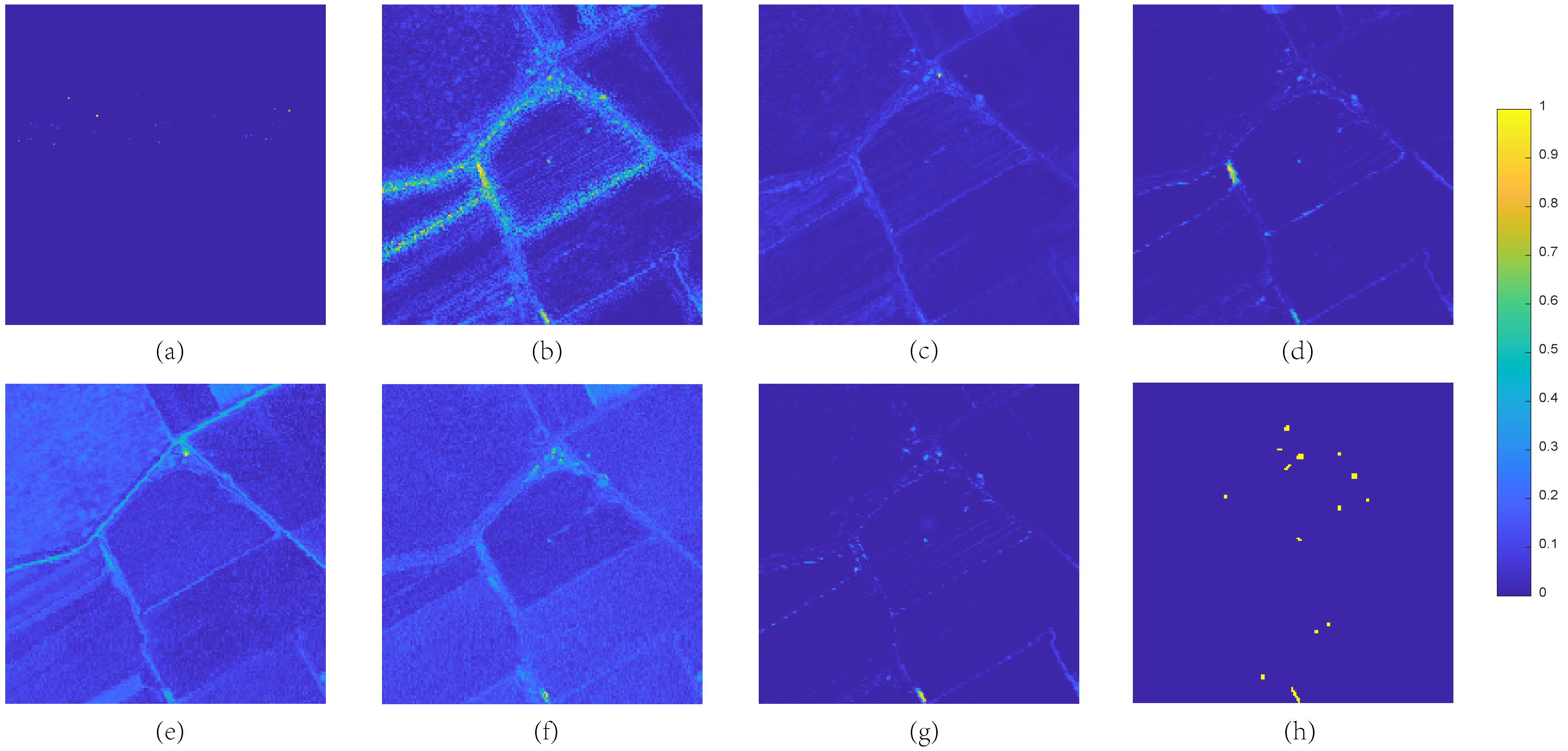
Figure 9 presents a depiction of the anomaly detection results on Salinas scene data. The anomaly detection result of LRX is the worst, and most of the anomalies are not detected. Compared with MC-AEN, Auto-AD and the proposed HAD-ASDR, BJSR, DeCNNAD and LRSNCR have higher false detection rates, which detect some background pixels as anomalies by mistake. It is obvious that the responses of the background of BJSR, DeCNNAD and LRSNCR are stronger than those of MC-AEN, Auto-AD and the proposed HAD-ASDR. It means the reconstruction error values of the background in BJSR, DeCNNAD and LRSNCR are too large, which makes it difficult to seperate anomalies from the background. Compared with MC-AEN, Auto-AD, the proposed HAD-ASDR has lower false-positive and miss-positive detection rates. It can be observed that the response of the background of the proposed HAD-ASDR is weaker than that of the other six methods, while the vast majority of anomalies are also detected. It proves that the proposed HAD-ASDR has achieved the best result due to its more accurate background reconstruction and calculation of the reconstructed errors based on the spectral intensity and angle.

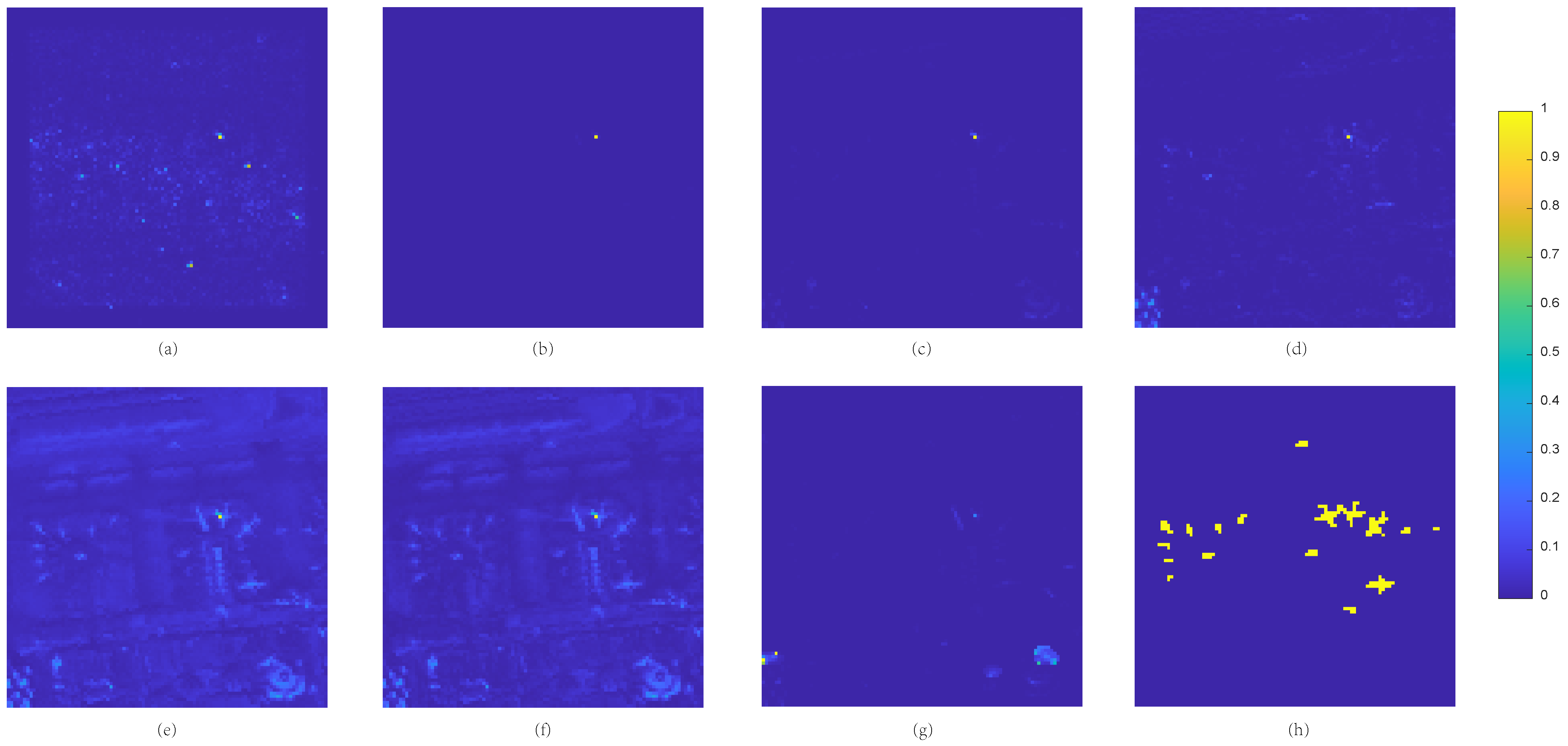
Figure 10 shows the anomaly detection results on Abu-airport-3 data. The performance of the proposed HAD-ASDR method and the comparison methods on Abu-airport-3 data is not very satisfactory. BJSR and MC-AEN only detect a small portion of anomalies. LRX, Auto-AD, and the proposed HAD-ASDR detect more anomalies compared to BJSR and MC-AEN. DeCNNAD and LRSNCR methods have better detection performance than other methods. The detection performance of the proposed HAD-ASDR method is lower than DeCNNAD and LRSNCR, with a relatively higher missed detection rate. As the background of these data is an airport with relatively uniform land cover types, the proposed method focuses on the diversity and complexity of land cover types in the background when constructing the background model.

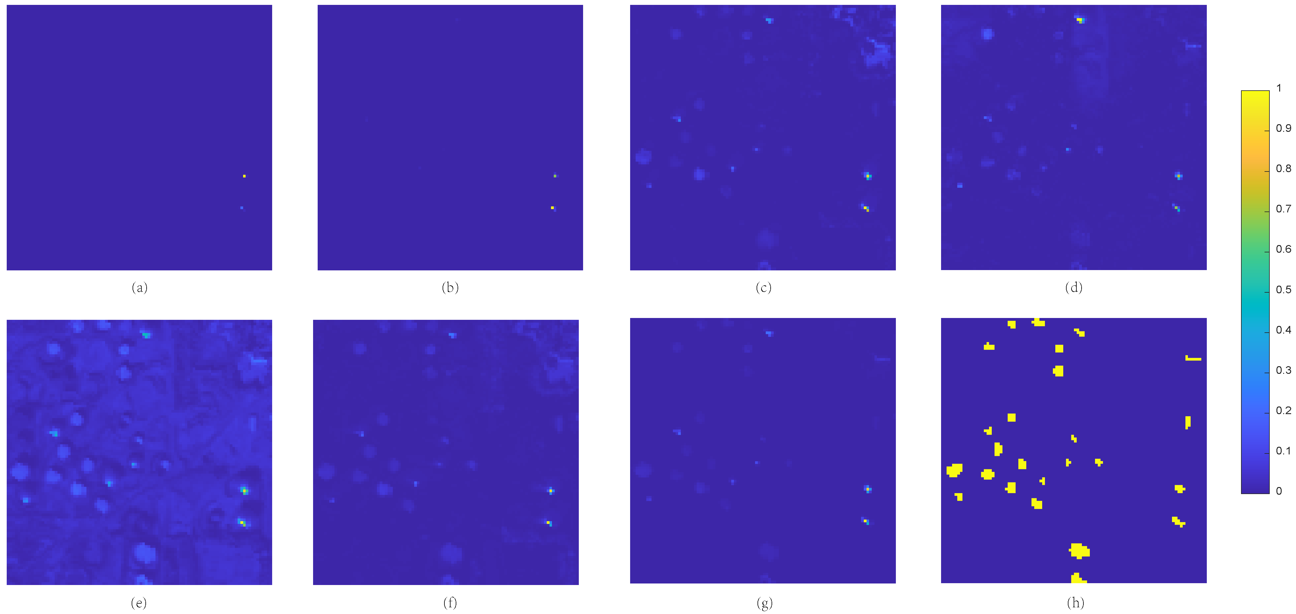
Figure 11 illustrates the anomaly detection results on the Abu-urban-4 data. The detection results of LRX and BJSR methods are not satisfactory, as they fail to detect many anomalies. The MC-AEN, Auto-AD, and LRSNCR exhibits better detection performance for anomalies, but some background pixels are still misclassified as anomalies. The DeCNNAD method has a higher false alarm rate compared to other methods. The proposed HAD-ASDR achieves lower false and missed detection rates. The ASDRM module employs the attention mechanism and spectral difference strategy to generate a noise distribution that considers the diversity and complexity of land cover types in the background. It can guide the construction of a more accurate background model, resulting in improved HAD performance.

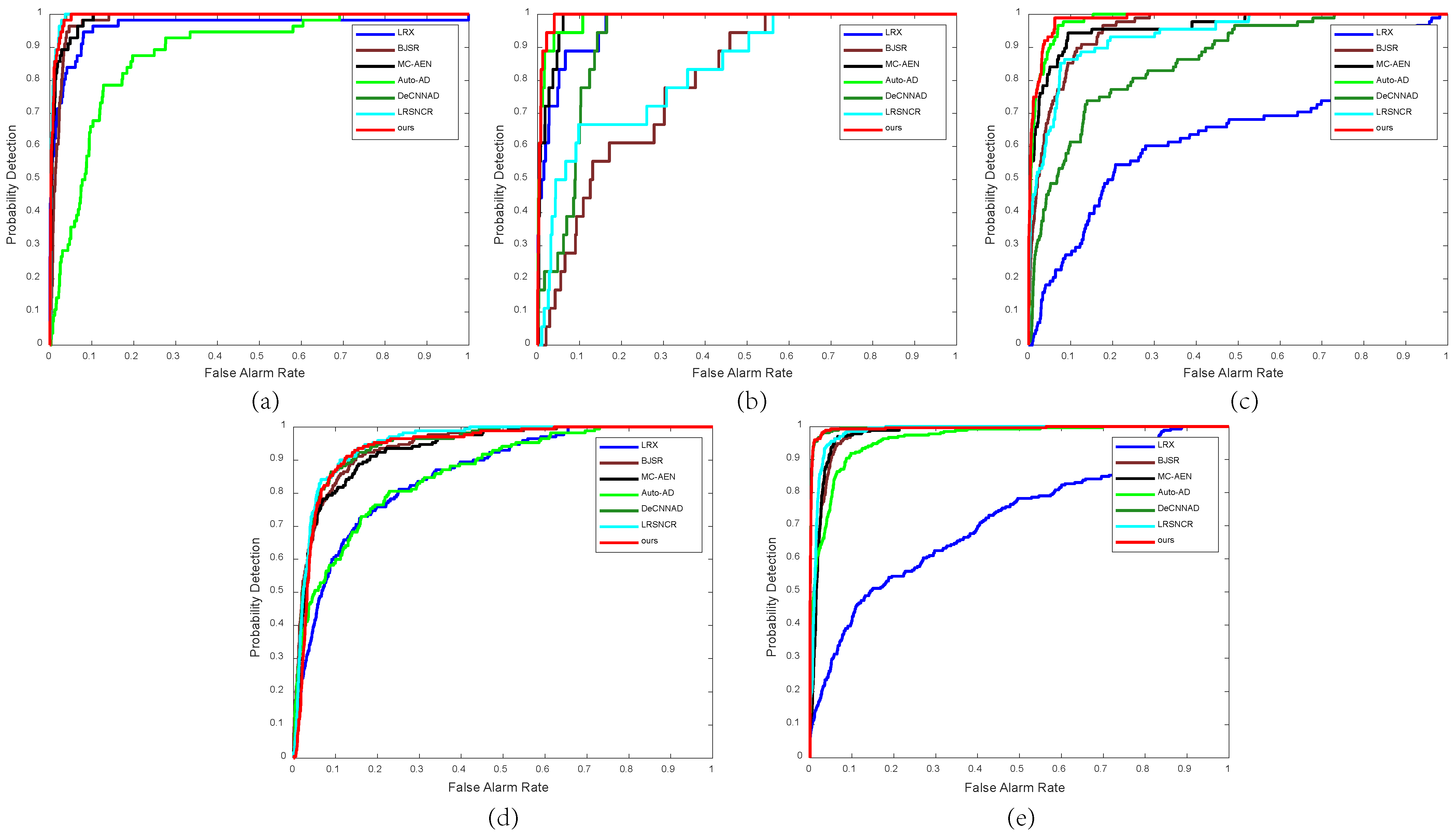
ROC curves for the HAD-ASDR algorithm and six comparison methods on five data sets are displayed in Figure 12. The ROC curve of the proposed HAD-ASDR is either above or equivalent to those of the comparison methods, which indicates that the proposed method achieves better or comparable HAD performance.

The effectiveness of the HAD-ASDR algorithm and six comparison methods are validated quantitatively through the calculation of AUC values on five data sets that are illustrated in

Table 2. AUC values for the five data on the comparison methods.

Dataset	LRX	BJSR	MC-AEN	Auto-AD	DeCNNAD	LRSNCR	HAD-ASDR
AVIRIS airplane data	0.8976	0.9810	0.9871	0.8822	0.9937	0.9938	0.9931
HYDICE urban data	0.9214	0.7988	0.9836	0.9875	0.9856	0.8362	0.9930
Salinas scene data	0.7595	0.9533	0.9608	0.9831	0.8609	0.9377	0.9863
Abu-airport-3 data	0.8587	0.9401	0.9335	0.8637	0.9463	0.9526	0.9408
Abu-urban-4 data	0.7219	0.9796	0.9774	0.9626	0.9955	0.9844	0.9955
Average AUC value	0.8318	0.9310	0.9685	0.9358	0.9564	0.9410	0.9817

. The AUC values of the proposed HAD-ASDR method are $0.9931$, $0.9930$, $0.9863$, $0.9408$ and $0.9955$ for AVIRIS airplane, HYDICE urban, Salinas scene, Abu-airport-3 and Abu-urban-4 data sets, respectively. The size of anomalies in the HYDICE urban data is small. The AUC values of BJSR and LRSNCR are $0.7988$ and $0.8362$, respectively, which are lower than those of LRX, MC-AEN and DeCNNAD. This is because LRX, MC-AEN and DeCNNAD take the local or priori information into account when calculating the reconstruction errors. Due to the suppression of the background by the adaptive-weighted loss function, the AUC value of Auto-AD is $0.9875$, which is higher than other comparison methods. The proposed HAD-ASDR achieves the highest AUC values on the HYDICE urban data. This is because the noise distribution of the background generated by ASDR is more matchable to the background, and the reconstructed errors are calculated taking both spectral intensity and angle into account. The types of anomalies in Salinas scene data are more complex than those in AVIRIS airplane data and HYDICE urban data. The proposed HAD-ASDR achieves higher AUC values than six other existing comparison methods, which proves that the proposed HAD-ASDR has better detection performance in relatively complex scenarios than other comparison methods.

In order to verify the stability of the proposed HAD-ASDR method and comparison methods on different data sets, the average AUC values for all methods are calculated on five data sets and displayed in the last row of Table 2. The proposed HAD-ASDR method achieves the highest average AUC value of 0.9817, with an improvement of 0.0253. It demonstrates that the proposed HAD-ASDR method has better or comparable HAD results on all five data sets and exhibits the best stability in comparison to other methods.

4.5. Algorithm Time Cost

In this section, the proposed algorithm is compared with six other methods to evaluate its time cost. The experiment was conducted on five different data sets, and the results are presented in

Table 3. The algorithm time cost of different methods on the five data sets (seconds).

Dataset	LRX	BJSR	MC-AEN	Auto-AD	DeCNNAD	LRSNCR	HAD-ASDR
AVIRIS airplane data	34.81	3085.96	214.05	38.57	34.27	20.52	126.54
HYDICE urban data	61.67	6958.46	482.01	28.66	27.96	29.68	117.87
Salinas scene data	131.60	9944.59	689.31	35.97	28.66	22.57	125.67
Abu-airport-3 data	44.88	3071.55	213.25	30.59	29.14	19.77	116.70
Abu-urban-4 data	42.46	3140.95	215.52	31.25	25.63	21.05	119.66
Average time	63.08	5240.30	362.82	33.08	29.13	22.72	121.29

.

Table 3 shows the average running time for all anomaly detection methods, with values of 63.08, 5240.30, 362.82, 33.08, 29.13, 22.72 and 121.29 seconds for LRX, BJSR, MC-AEN, Auto-AD, DeCNNAD, LRSNCR and the proposed HAD-ASDR, respectively. In terms of time efficiency, DeCNNAD and LRSNCR appear to yield the best results, as they utilize pre-trained optimal models for detection, which only includes the time cost of testing and excludes the training time. In contrast, the proposed HAD-ASDR can detect anomalies directly without prior model training, so its algorithm execution contains both training and testing time. Taking into account both the detection performance and the time required for anomaly detection, the proposed HAD-ASDR achieves the satisfactory performance.

4.6. Ablation Study

4.6.1. The Effective of ASDR

The following ablation experiments are designed to validate the ASDR module’s effectiveness.

The ASDR module is removed, and the noise generated from a uniform distribution in the range [0, 1] is fed to the CAE-BRM module as input, denoted as “HAD-ASDR wo ASDR”. The ablation experiments are carried out on AVIRIS airplane data, HYDICE urban data, Salinas scene data, Abu-airport-3 data and Abu-urban-4 data. The anomaly detection results are displayed in Figure 13a. The blue color indicates the anomaly detection results of the HAD-ASDR wo ASDR method. The red color represents the anomaly detection results of the proposed HAD-ASDR method.

The AUC values of the HAD-ASDR and ASDR method on the five data sets reaches $0.9298$, $0.9616$, $0.9401$, $0.8900$, $0.9526$, respectively. Meanwhile, the AUC values of the HAD-ASDR method reaches $0.9931$, $0.9930$, $0.9863$, $0.9408$ and $0.9955$. After the ASDR model is removed, it is obvious that the AUC values of the HAD-ASDR wo ASDR model decreased by $0.0633$, $0.0314$, $0.0462$, $0.0508$ and $0.0429$ for AVIRIS airplane data, HYDICE urban data, Salinas scene data, Abu-airport-3 data and Abu-urban-4 data, respectively. It can demonstrate that the proposed ASDR module can generate the noise distribution of the background that matches better with the background, which will lead to the reconstructed background being more accurate, and achieve higher anomaly detection results.

4.6.2. The Effective of JSIA-ADM

The following ablation experiments are designed to validate the effectiveness of JSIA-ADM. The reconstruction error is calculated only based on the spectral intensity in the JSIA-ADM, and the Spectral Angle (SA) is not considered, denoted as “JSIA-ADM wo SA”. That means that only $RErro{r}_{Intensity}^i$ is employed to detect anomalies in the JSIA-ADM wo SA method. The ablation experimental results on five data sets are shown in Figure 13b. The blue color indicates that the reconstruction error $RErro{r}_{Intensity}^i$ in Equation (7) in the JSIA-ADM wo SA method is used to detect anomalies. The red color means the reconstruction errors $RErro{r}^i$ in Equation (6) are employed to detect anomalies, where $\alpha$ is $0.0001$.

The AUC values for ablation experiments on five data sets of the comparison JSIA-ADM wo SA method and the proposed HAD-ASDR are illustrated in Figure 13b. The AUC values of the JSIA-ADM wo SA method reaches $0.9871$, $0.9732$, $0.9856$, $0.9067$, $0.9843$ for the five data sets, respectively. Meanwhile, the AUC values of the HAD-ASDR method on the five data sets reaches $0.9931$, $0.9930$, $0.9863$, $0.9408$ and $0.9955$, respectively. After SA is considered when calculating the total reconstruction errors, it can be observed that the AUC values of the proposed HAD-ASDR increase by $0.0060$, $0.0198$, $0.0007$, $0.0341$ and $0.0112$ for AVIRIS airplane data, HYDICE urban data, Salinas scene data, Abu-airport-3 data and Abu-urban-4 data, respectively. It proves that when the reconstruction error $RErro{r}^i$ in Equation (6) is utilized in the proposed JSIA-ADM method to detect anomalies, the proposed JSIA-ADM can achieve a better anomaly detection performance. It is because the reconstruction errors $RErro{r}^i$ are calculated from both spectral intensity and angle perspectives, and the spectral angle provides a similarity measure of the spectral curve.

4.6.3. The Effectiveness of the Penalty Parameter α

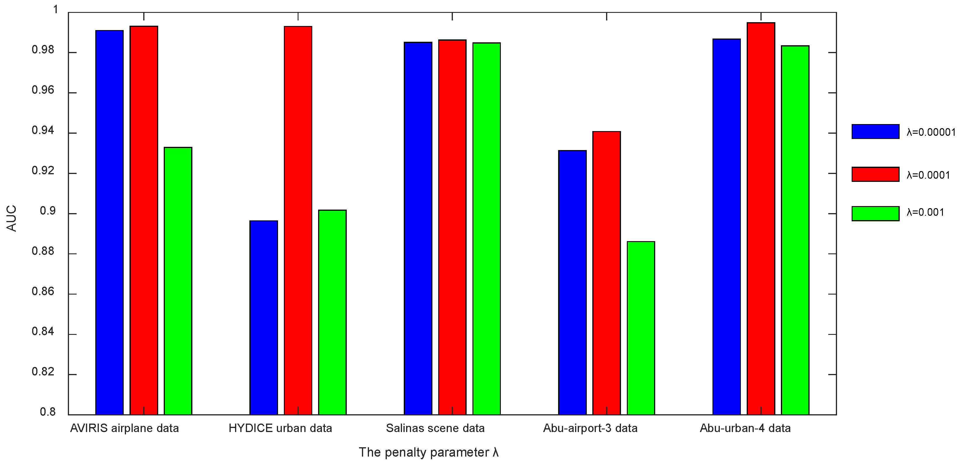
This section evaluates the impact of the penalty parameter $\alpha$, as defined in Equation (6), on the performance of anomaly detection. The penalty parameter $\alpha$ is designed to balance the contributions of $RErro{r}_{Intensity}^i$ and $RErro{r}_{Angle}^i$ to the total reconstruction error $RErro{r}^i$. Since the spectral intensity can provide the critical spectral information, which is often utilized in HAD, the penalty parameter of $RErro{r}_{Intensity}^i$ is set to 1. The spectral angle can also be used to make the reconstruction error more accurate. Hence, the penalty parameter $\alpha$ is adjusted to seek the best combination of $RErro{r}_{Intensity}^i$ and $RErro{r}_{Angle}^i$. The penalty parameters $\alpha$ are set to $0.00001$, $0.0001$ and $0.001$, respectively. The impact of the penalty parameter $\alpha$ on the anomaly detection performance is verified on five data sets, and the AUC values are illustrated in Figure 14.

As shown in Figure 14, the experimental results display a convex function that initially increases and then decreases as the value of $\alpha$ ranges from $0.00001$ to $0.001$. When $\alpha$ is set to $0.00001$, the AUC values for the five data sets are $0.9298$, $0.9616$, $0.9401$, $0.9313$, $0.8861$. With $\alpha$ at $0.0001$, the AUC values for the five data sets are $0.9931$, $0.9930$, $0.9863$, $0.9408$ and $0.9955$. When $\alpha$ is set to $0.001$ in Equation (6), the proposed HAD-ASDR achieves AUC values of $0.9871$, $0.9732$, $0.9856$, $0.8861$ and $0.9834$ of AUC values on five data sets. It can obvious that the AUC values are highest when $\alpha$ = 0.0001 for all five data sets. Therefore, the penalty parameter $\alpha$ is set to $0.0001$ on five data sets in our experiment.

5. Conclusions

The proposed attention-aware spectral difference representation network for HAD aims to improve the HAD accuracy by reconstructing a more accurate background with various and complex land cover types. The proposed HAD-ASDR contains three components: ASDRM, CAE-BRM and JSIA-ADM. ASDRM uses a spectral channel attention block, a spatial attention block, an auto-encoder block as the backbone and employs two difference operations to generate the noise distribution that better matches the background. CAE-BRM uses the convolutional auto-encoder with the skip connections as the backbone to reconstruct the more accurate background by taking the spatial and intermediate information into account. JSIA-ADM calculates the reconstruction errors based on both spectral intensity and angle to obtain a more accurate anomaly detection map. Through extensive experimentation on five real data sets, the proposed HAD-ASDR has consistently shown superior or comparable detection performance, achieving higher or comparable AUC values. The proposed HAD-ASDR outperforms all other methods on the relatively complex data sets of HYDICE Urban, Salinas Scene and Abu-urban-4 data sets, with respective AUC values of $0.9930$, $0.9863$ and $0.9955$. Furthermore, the average AUC value of our proposed method on the five data sets is significantly higher than that of other methods, with an improvement of $0.0253$. The experimental results demonstrate that the proposed HAD-ASDR method achieves better or comparable HAD results on all five data sets and exhibits the best stability in comparison to other methods.

References

1. Chang, C.I.; Chiang, S.S. Anomaly detection and classification for hyperspectral imagery. IEEE Trans. Geosci. Remote Sens. 2002, 40, 1314–1325. [Google Scholar] [CrossRef]
2. Liu, S.; Marinelli, D.; Bruzzone, L.; Bovolo, F. A review of change detection in multitemporal hyperspectral images: Current techniques, applications, and challenges. IEEE Geosci. Remote Sens. Mag. 2019, 7, 140–158. [Google Scholar] [CrossRef]
3. Hu, X.; Xie, C.; Fan, Z.; Duan, Q.; Zhang, D.; Jiang, L.; Wei, X.; Hong, D.; Li, G.; Zeng, X.; et al. Hyperspectral anomaly detection using deep learning: A review. Remote Sens. 2022, 14, 1973. [Google Scholar] [CrossRef]
4. Theiler, J.; Wohlberg, B. Local coregistration adjustment for anomalous change detection. IEEE Trans. Geosci. Remote Sens. 2012, 50, 3107–3116. [Google Scholar] [CrossRef]
5. Khazai, S.; Safari, A.; Mojaradi, B.; Homayouni, S. An approach for subpixel anomaly detection in hyperspectral images. IEEE J. Sel. Top. Appl. Earth Obs. Remote Sens. 2012, 6, 769–778. [Google Scholar] [CrossRef]
6. Zhang, X.; Wen, G.; Dai, W. A tensor decomposition-based anomaly detection algorithm for hyperspectral image. IEEE Trans. Geosci. Remote Sens. 2016, 54, 5801–5820. [Google Scholar] [CrossRef]
7. Chalapathy, R.; Chawla, S. Deep learning for anomaly detection: A survey. arXiv 2019, arXiv:1901.03407. [Google Scholar]
8. Nayak, R.; Pati, U.C.; Das, S.K. A comprehensive review on deep learning-based methods for video anomaly detection. Image Vis. Comput. 2021, 106, 104078. [Google Scholar] [CrossRef]
9. Reed, I.S.; Yu, X. Adaptive multiple-band CFAR detection of an optical pattern with unknown spectral distribution. IEEE Trans. Acoust. Speech Signal Process. 1990, 38, 1760–1770. [Google Scholar] [CrossRef]
10. Zhao, C.; Li, X.; Ren, J.; Marshall, S. Improved sparse representation using adaptive spatial support for effective target detection in hyperspectral imagery. Int. J. Remote Sens. 2013, 34, 8669–8684. [Google Scholar] [CrossRef]
11. Du, B.; Zhang, L. Random-selection-based anomaly detector for hyperspectral imagery. IEEE Trans. Geosci. Remote Sens. 2010, 49, 1578–1589. [Google Scholar] [CrossRef]
12. Hinton, G.E. Deep belief networks. Scholarpedia 2009, 4, 5947. [Google Scholar] [CrossRef]
13. Tschannen, M.; Bachem, O.; Lucic, M. Recent advances in autoencoder-based representation learning. arXiv 2018, arXiv:1812.05069. [Google Scholar]
14. Gu, J.; Wang, Z.; Kuen, J.; Ma, L.; Shahroudy, A.; Shuai, B.; Liu, T.; Wang, X.; Wang, G.; Cai, J.; et al. Recent advances in convolutional neural networks. Pattern Recognit. 2018, 77, 354–377. [Google Scholar] [CrossRef]
15. Medsker, L.R.; Jain, L. Recurrent neural networks. Des. Appl. 2001, 5, 64–67. [Google Scholar]
16. Graves, A.; Graves, A. Long Short-Term Memory. Supervised Sequence Labelling with Recurrent Neural Networks. Ph.D. Thesis, Technical University of Munich, Munich, Germany, 2012; pp. 37–45. [Google Scholar]
17. Creswell, A.; White, T.; Dumoulin, V.; Arulkumaran, K.; Sengupta, B.; Bharath, A.A. Generative adversarial networks: An overview. IEEE Signal Process. Mag. 2018, 35, 53–65. [Google Scholar] [CrossRef]
18. Ma, N.; Peng, Y.; Wang, S.; Leong, P.H. An unsupervised deep hyperspectral anomaly detector. Sensors 2018, 18, 693. [Google Scholar] [CrossRef]
19. Su, H.; Wu, Z.; Zhang, H.; Du, Q. Hyperspectral anomaly detection: A survey. IEEE Geosci. Remote Sens. Mag. 2021, 10, 64–90. [Google Scholar] [CrossRef]
20. Xu, Y.; Zhang, L.; Du, B.; Zhang, L. Hyperspectral anomaly detection based on machine learning: An overview. IEEE J. Sel. Top. Appl. Earth Obs. Remote Sens. 2022, 15, 3351–3364. [Google Scholar] [CrossRef]
21. Zheng, X.; Chen, W.; Lu, X. Spectral super-resolution of multispectral images using spatial–spectral residual attention network. IEEE Trans. Geosci. Remote Sens. 2022, 60, 5404114. [Google Scholar] [CrossRef]
22. Kwon, H.; Nasrabadi, N.M. Kernel RX-algorithm: A nonlinear anomaly detector for hyperspectral imagery. IEEE Trans. Geosci. Remote Sens. 2005, 43, 388–397. [Google Scholar] [CrossRef]
23. Zhao, R.; Du, B.; Zhang, L. A robust nonlinear hyperspectral anomaly detection approach. IEEE J. Sel. Top. Appl. Earth Obs. Remote Sens. 2014, 7, 1227–1234. [Google Scholar] [CrossRef]
24. Su, H.; Wu, Z.; Zhu, A.X.; Du, Q. Low rank and collaborative representation for hyperspectral anomaly detection via robust dictionary construction. ISPRS J. Photogramm. Remote Sens. 2020, 169, 195–211. [Google Scholar] [CrossRef]
25. Li, J.; Zhang, H.; Zhang, L.; Ma, L. Hyperspectral anomaly detection by the use of background joint sparse representation. IEEE J. Sel. Top. Appl. Earth Obs. Remote Sens. 2015, 8, 2523–2533. [Google Scholar] [CrossRef]
26. Li, S.; Wang, W.; Qi, H.; Ayhan, B.; Kwan, C.; Vance, S. Low-rank tensor decomposition based anomaly detection for hyperspectral imagery. In Proceedings of the 2015 IEEE International Conference on Image Processing (ICIP), Quebec City, QC, Canada, 27–30 September 2015; pp. 4525–4529. [Google Scholar]
27. Kang, X.; Zhang, X.; Li, S.; Li, K.; Li, J.; Benediktsson, J.A. Hyperspectral anomaly detection with attribute and edge-preserving filters. IEEE Trans. Geosci. Remote Sens. 2017, 55, 5600–5611. [Google Scholar] [CrossRef]
28. Fu, X.; Jia, S.; Zhuang, L.; Xu, M.; Zhou, J.; Li, Q. Hyperspectral anomaly detection via deep plug-and-play denoising CNN regularization. IEEE Trans. Geosci. Remote Sens. 2021, 59, 9553–9568. [Google Scholar] [CrossRef]
29. Bati, E.; Çalışkan, A.; Koz, A.; Alatan, A.A. Hyperspectral anomaly detection method based on auto-encoder. In Proceedings of the Image and Signal Processing for Remote Sensing XXI., Virtual, 10 November 2015; SPIE: Washington, DC, USA, 2015; Volume 9643, pp. 220–226. [Google Scholar]
30. Xie, W.; Liu, B.; Li, Y.; Lei, J.; Du, Q. Autoencoder and adversarial-learning-based semisupervised background estimation for hyperspectral anomaly detection. IEEE Trans. Geosci. Remote Sens. 2020, 58, 5416–5427. [Google Scholar] [CrossRef]
31. Chang, S.; Du, B.; Zhang, L. A sparse autoencoder based hyperspectral anomaly detection algorihtm using residual of reconstruction error. In Proceedings of the IGARSS 2019 IEEE International Geoscience and Remote Sensing Symposium, Yokohama, Japan, 28 July–2 August 2019; pp. 5488–5491. [Google Scholar]
32. Jiang, T.; Li, Y.; Xie, W.; Du, Q. Discriminative reconstruction constrained generative adversarial network for hyperspectral anomaly detection. IEEE Trans. Geosci. Remote Sens. 2020, 58, 4666–4679. [Google Scholar] [CrossRef]
33. Zhu, D.; Du, B.; Zhang, L. EDLAD: An encoder-decoder long short-term memory network-based anomaly detector for hyperspectral images. In Proceedings of the 2021 IEEE International Geoscience and Remote Sensing Symposium IGARSS, Brussels, Belgium, 11–16 July 2021; pp. 4412–4415. [Google Scholar]
34. Zheng, X.; Chen, X.; Lu, X.; Sun, B. Unsupervised change detection by cross-resolution difference learning. IEEE Trans. Geosci. Remote Sens. 2021, 60, 5606616. [Google Scholar] [CrossRef]
35. Zhang, Y. A Better Autoencoder for Image: Convolutional Autoencoder. In Proceedings of the ICONIP17-DCEC. 2018. Available online: http://users.cecs.anu.edu.au/Tom.Gedeon/conf/ABCs2018/paper/ABCs2018_paper_58.pdf (accessed on 23 March 2017).
36. Zheng, X.; Gong, T.; Li, X.; Lu, X. Generalized scene classification from small-scale datasets with multitask learning. IEEE Trans. Geosci. Remote Sens. 2021, 60, 5609311. [Google Scholar] [CrossRef]
37. Zheng, X.; Wang, B.; Du, X.; Lu, X. Mutual attention inception network for remote sensing visual question answering. IEEE Trans. Geosci. Remote Sens. 2021, 60, 5606514. [Google Scholar] [CrossRef]
38. Zhao, W.; Guo, Z.; Yue, J.; Zhang, X.; Luo, L. On combining multiscale deep learning features for the classification of hyperspectral remote sensing imagery. Int. J. Remote Sens. 2015, 36, 3368–3379. [Google Scholar] [CrossRef]
39. Hosseiny, B.; Shah-Hosseini, R. A hyperspectral anomaly detection framework based on segmentation and convolutional neural network algorithms. Int. J. Remote Sens. 2020, 41, 6946–6975. [Google Scholar] [CrossRef]
40. Shi, Y.; Li, J.; Yin, Y.; Xi, B.; Li, Y. Hyperspectral target detection with macro-micro feature extracted by 3-D residual autoencoder. IEEE J. Sel. Top. Appl. Earth Obs. Remote Sens. 2019, 12, 4907–4919. [Google Scholar] [CrossRef]
41. Zheng, X.; Sun, H.; Lu, X.; Xie, W. Rotation-invariant attention network for hyperspectral image classification. IEEE Trans. Image Process. 2022, 31, 4251–4265. [Google Scholar] [CrossRef]
42. Chen, L.; Maddox, R.K.; Duan, Z.; Xu, C. Hierarchical cross-modal talking face generation with dynamic pixel-wise loss. In Proceedings of the IEEE/CVF Conference on Computer Vision and Pattern Recognition, Long Beach, CA, USA, 15–20 June 2019; pp. 7832–7841. [Google Scholar]
43. Cai, W.; Wei, Z. Remote sensing image classification based on a cross-attention mechanism and graph convolution. IEEE Geosci. Remote Sens. Lett. 2020, 19, 8002005. [Google Scholar] [CrossRef]
44. Ju, M.; Luo, J.; Wang, Z.; Luo, H. Adaptive feature fusion with attention mechanism for multi-scale target detection. Neural Comput. Appl. 2021, 33, 2769–2781. [Google Scholar] [CrossRef]
45. Nasrabadi, N.M. Regularization for spectral matched filter and RX anomaly detector. In Proceedings of the Algorithms and Technologies for Multispectral, Hyperspectral, and Ultraspectral Imagery XIV, Virtual, 2 August 2002; SPIE: Washington, DC, USA, 2008; Volume 6966, pp. 28–39. [Google Scholar]
46. Lu, X.; Zhang, W.; Huang, J. Exploiting embedding manifold of autoencoders for hyperspectral anomaly detection. IEEE Trans. Geosci. Remote Sens. 2019, 58, 1527–1537. [Google Scholar] [CrossRef]
47. Wang, S.; Wang, X.; Zhang, L.; Zhong, Y. Auto-AD: Autonomous hyperspectral anomaly detection network based on fully convolutional autoencoder. IEEE Trans. Geosci. Remote Sens. 2021, 60, 5503314. [Google Scholar] [CrossRef]
48. Yao, W.; Li, L.; Ni, H.; Li, W.; Tao, R. Hyperspectral anomaly detection based on improved RPCA with non-convex regularization. Remote Sens. 2022, 14, 1343. [Google Scholar] [CrossRef]
Figure 1. The flowchart of Hyperspectral Anomaly Detection method based on Attention-aware Spectral Difference Representation (HAD-ASDR).
Remotesensing 15 02652 g001
Figure 2. (a) The pseudo-color image of AVIRIS airplane data. (b) The ground truth.
Remotesensing 15 02652 g002
Figure 3. (a) The pseudo-color image of HYDICE urban data. (b) The ground truth.
Remotesensing 15 02652 g003
Figure 4. (a) The pseudo-color image of Salinas scene data. (b) The ground truth.
Remotesensing 15 02652 g004
Figure 5. (a) The pseudo-color image of Abu-airport-3 data. (b) The ground truth.
Remotesensing 15 02652 g005
Figure 6. (a) The pseudo-color image of Abu-urban-4 data. (b) The ground truth.
Remotesensing 15 02652 g006
Figure 7. The visualization of the anomaly detection results on AVIRIS airplane data set. (a) LRX. (b) BJSR. (c) MC-AEN. (d) Auto-AD. (e) DeCNNAD. (f) LRSNCR. (g) Ours. (h) Ground truth.
Remotesensing 15 02652 g007
Figure 8. The visualization of the anomaly detection results on HYDICE urban data set. (a) LRX. (b) BJSR. (c) MC-AEN. (d) Auto-AD. (e) DeCNNAD. (f) LRSNCR. (g) Ours. (h) Ground truth.
Remotesensing 15 02652 g008
Figure 9. The visualization of the anomaly detection results on Salinas scene set. (a) LRX. (b) BJSR. (c) MC-AEN. (d) Auto-AD. (e) DeCNNAD. (f) LRSNCR. (g) Ours. (h) Ground truth.
Remotesensing 15 02652 g009
Figure 10. The visualization of the anomaly detection results on Abu-airport-3 set. (a) LRX. (b) BJSR.(c) MC-AEN. (d) Auto-AD. (e) DeCNNAD. (f) LRSNCR. (g) Ours. (h) Ground truth.
Remotesensing 15 02652 g010
Figure 11. The visualization of the anomaly detection results on Abu-urban-4 set. (a) LRX. (b) BJSR. (c) MC-AEN. (d) Auto-AD. (e) DeCNNAD. (f) LRSNCR. (g) Ours. (h) Ground truth.
Remotesensing 15 02652 g011
Figure 12. ROC curves for the proposed HAD-ASDR and six comparison methods on the five data sets. (a) AVIRIS airplane data. (b) HYDICE urban data. (c) Salinas scene data. (d) Abu-airport-3 data. (e) Abu-urban-4 data.
Remotesensing 15 02652 g012
Figure 13. The result of ablation experiments. (a) AUC values for HAD-ASDR wo ASDR and HAD-ASDR. (b) AUC values for JSIA-ADM wo SA and HAD-ASDR.
Remotesensing 15 02652 g013
Figure 14. AUC values with the change of the sale of the penalty parameter α .
Remotesensing 15 02652 g014