Knowledge Enhanced Neural Networks for Point Cloud Semantic Segmentation

Abstract

Deep learning approaches have sparked much interest in the AI community during the last decade, becoming state-of-the-art in domains such as pattern recognition, computer vision, and data analysis. However, these methods are highly demanding in terms of training data, which is often a major issue in the geospatial and remote sensing fields. One possible solution to this problem comes from the Neuro-Symbolic Integration field (NeSy), where multiple methods have been defined to incorporate background knowledge into the neural network’s learning pipeline. One such method is KENN (Knowledge Enhanced Neural Networks), which injects logical knowledge into the neural network’s structure through additional final layers. Empirically, KENN showed comparable or better results than other NeSy frameworks in various tasks while being more scalable. Therefore, we propose the usage of KENN for point cloud semantic segmentation tasks, where it has immense potential to resolve issues with small sample sizes and unbalanced classes. While other works enforce the knowledge constraints in post-processing, to the best of our knowledge, no previous methods have injected inject such knowledge into the learning pipeline through the use of a NeSy framework. The experiment results over different datasets demonstrate that the introduction of knowledge rules enhances the performance of the original network and achieves state-of-the-art levels of accuracy, even with subideal training data.

1. Introduction

The introduction of semantic information using AI approaches represents a key step in the understanding of point cloud datasets. In the geospatial and remote sensing fields, there is still an open debate between standard machine learning (ML) approaches and more innovative deep learning (DL) methods for point cloud semantic segmentation [1]. Although ML approaches have proven to perform effectively in various scenarios [2,3], they still generate some inevitable noise, resulting in unsmooth outputs since the segmentation does not consider contextual features of points [4]. On the other hand, DL strictly depends on the quality and amount of available training data. Optimal results have been achieved in recent years [5] thanks also to the growing availability of different point cloud benchmarks [3,6,7,8,9]. However, point cloud semantic segmentation still faces a major challenge in dealing with unbalanced classes, which refer to a situation where the number of points belonging to different semantic classes is highly imbalanced. For instance, in a street scene, the majority of points may belong to the road surface, while the number of points belonging to other classes, such as pedestrians or cars, may be much smaller. To address this challenge, various methods have been proposed in the literature, including data augmentation [10,11], class weighting [12,13], and oversampling/undersampling techniques [14,15]. However, it remains an open research problem to find an effective and efficient method that can handle unbalanced classes in the context of point cloud semantic segmentation. In this paper, we propose a novel method that explicitly addresses the issue of unbalanced classes by applying knowledge-based rules at various levels of the segmentation pipeline. Our approach is motivated by the fact that point cloud semantic segmentation can benefit from the use of prior knowledge or domain-specific rules, especially in cases where the distribution of classes is highly imbalanced. Previous research, for example, has demonstrated that the introduction of a-priori knowledge in the form of hand-crafted features, allows for an improvement in the prediction results [1,16]. Others have proposed the introduction of a-posteriori rules to correct the label predictions [17]. In this study, for the first time, knowledge-based rules are introduced within the DL-based segmentation pipeline of 3D point clouds using a neuro-symbolic (NeSy) approach. NeSy concerns the combination of artificial neural networks with symbolic methods. In particular, we use KENN (Knowledge Enhanced Neural Networks) [18,19], a method that incorporates logical background knowledge into neural networks in the form of an additional differentiable layer on top of the architecture. By leveraging such rules, our method can guide the segmentation process towards the identification of points that belong to minority classes, even in the presence of noisy or ambiguous data. To evaluate the effectiveness of our approach, three public benchmark datasets have been considered: Vaihingen 3D (V3D) [20], Hessigheim 3D (H3D) [3], and Stanford Large-Scale 3D Indoor Spaces (S3DIS) [21]. Additionally, an internal dataset, named FBK cable/powerlines, has been used for tuning the approach.

In summary, our contributions are:

1.

The theoretical framework and code implementation of neuro-symbolic logic for 3D point cloud semantic segmentation;

2.

Extensive study of training data shortcomings and remedies;

3.

Empirical study on three benchmarks and one internal dataset to validate the performance of knowledge enhancement in a neural network.

The paper is organized as follows. Section 2 presents an overview of the field’s related work. Section 3 describes in detail the methodology proposed, while the experiments conducted and the results achieved are shown in Section 4. In Section 5, we present our critical observations, and finally, in Section 6, the prospective future works.

2. Related Work

For the understanding of this study, in the following sub-sections, we will briefly summarize the relevant work in the fields of both semantic segmentation (Section 2.1) and neuro-symbolic (or neural-symbolic) integration (Section 2.2).

2.1. Point-Wise Semantic Segmentation

Point-wise semantic segmentation assigns a class label to every point of a point cloud. Compared with other point cloud semantic segmentation strategies such as voxel-based [22,23] or projection-based [24,25] methods, point-wise labeling is extremely challenging as methods have to directly operate on the unprocessed 3D information [26]. Initially, machine learning-based methods such as Random Forests, Support Vector Machines, Markov random fields were proposed to process this information. These methods employ radiometric and geometric features such as covariance features [17] and topological features [27] to better semantically segment point clouds. The features proved to be quite promising, but still, the methods struggled with interpreting scenes without explicit user knowledge.

In recent years, the state of the art has therefore switched to increasingly deep learning methods [28]. Early solutions included PointNet [29] and its successor PointNet++ [30], which tackled the dimensionality problem by using layered partitioning of the input point sets. Through the use of shared multilayer perceptrons, Pointnet/Pointnet++ learn per-point characteristics. Although computationally effective, this does not adequately represent each point’s wider context due to the layering. Subsequent works studied the convolution of 3D point sets, defining effective convolution kernels such as PointCNN [31] and KPConv [32]. With the introduction of RandlLA-Net [33], 3D semantic segmentation made significant progress in terms of speed and accuracy on large-scale datasets, thanks to the use of random sampling to greatly reduce point density while retaining prominent features with a designed local feature aggregator.

An alternative way of processing the irregular 3D data is to represent the point cloud as a graph to model the local geometric information between the points. For instance, in ECC [34], specific edge labels are proposed that filter weights conditioned on the neighborhood of each vertex. DGCNN [35] incorporates a similar graph structure that is dynamically updated by changing the set of k-nearest neighbors of a point from layer to layer of the network. Matrone et al. [1] demonstrate that combining DGCNN and heuristic 3D features can significantly improve the segmentation results.

Many studies have recently been focused on the use of Transformer architectures [36], the initially dominant framework in natural language processing [37], for point cloud semantic segmentation. Input (word) embedding, positional (order) encoding, and self-attention are the three basic modules of the decoder-encoder system known as Transformer. The self-attention module, which generates refined attention features for its input feature based on the global context, is the main part of the system. As described by Zhao et al. [38], since point clouds are simply sets that are irregularly embedded in a metric space, self-attention perfectly fits with the point cloud environment. For a comprehensive literature review about Transformers models in 3D point clouds, the authors refer to the recently published paper by Lu et al. [39]. For this study, we decided to start from the original version of Point Transformer (PT) for semantic segmentation proposed by Zhao et al. [38], as this architecture sets in 2021 the new state of the art on different public benchmarks such as the S3DIS dataset [26], Model-Net40 [40], and ShapeNetPart [41]. In the experiments that follow, the PT architecture is integrated with some background knowledge in the form of hand-crafted features and logic rules. For 3D object detection and semantic segmentation tasks, the use of hand-created features with neural networks [6,16,42], as well as the application of ontologies and logical rules [43,44,45], have already been shown to be effective. However, to the best of our knowledge, this is the first time that they have been combined and integrated together within a neural network.

2.2. Neuro-Symbolic Integration

Neuro-symbolic Integration (NeSy) is a sub-field of machine learning that aims to integrate the learning capabilities of neural networks with the reasoning abilities of symbolic frameworks [46]. NeSy approaches can be classified based on the role of symbolic knowledge: in some methods, such as $\delta ILP$ [47,48], the knowledge is learned from the data; in other approaches, such as DeepProbLog [49], the knowledge is used to infer new facts starting from initial facts produced by the neural network; finally, some methods interpret the knowledge as a set of constraints on the output of the neural network. This last type of integration is the one we consider in our work, since we are interested in exploiting prior knowledge to improve the performance of neural networks.

Many frameworks have been introduced to incorporate logical knowledge into neural networks, following mainly two strategies to incorporate the knowledge within neural networks. Based on the adopted strategy, we can classify the various approaches into two categories: loss-based and model-based methods. The former encompasses Logic Tensor Networks [50,51], Semantic-Based Regularization [52], and Semantic Loss [53] approaches. These frameworks incorporate knowledge into neural networks through a regularization term added to the loss function. Such a regularization enforces the domain knowledge to be satisfied. The knowledge is therefore used as an additional supervision that penalizes solutions that do not satisfy the given constraints. One of the limitations of this approach is that the knowledge is used only during training to guide learning. Upon inference, the loss is discarded along with the regularization term. Therefore, knowledge is not taken into consideration when performing inference. Moreover, it has been shown that loss-based methods are particularly useful in weakly supervised learning scenarios but struggle on fully supervised tasks [54]. This limitation motivates our choice of a model-based approach since point cloud semantic segmentation is a supervised learning task.

Model-based approaches inject knowledge directly into the structure of the neural network. Consequently, the knowledge is enforced both at training and inference time. Early attempts to inject knowledge into the structure of the NN consist of methods such as Knowledge-Based Artificial Neural Networks (KBANN) [55] and C-IL ${}^2$P [56], which codify the logical knowledge into the weights of the neural network. However, these methods are restricted to propositional logic, with no possibility of incorporating binary predicates into the given knowledge. This is a strong limitation, particularly in relational contexts, since the relations cannot be efficiently represented as propositions. For instance, in propositional logic, we need to define a proposition $Nea{r}_{a,b}$ for each pair of points $(a,b)$ to represent that a and b are close together. On the other hand, in First Order Logic (FOL), $Near(x,y)$ is a predicate, with x and y representing placeholders for each point in the dataset, resulting in a much more compact representation of the knowledge.

A more recent approach is Relational Neural Machines (RNM) [57], which perform an optimization process to combine the predictions of the neural network with the given knowledge. Among the advantages of this method is the ability to learn rules’ weights from the data. However, solving an optimization problem in the forward step of a neural network requires a huge computational effort, reducing the scalability of the approach. Iterative Local Refinement (ILR) [58] is another method that, similarly to RNM, optimizes knowledge satisfaction starting from the predictions of the neural network. It defines a Back-Propagation algorithm that converges very quickly to a local optimum solution. Still, the work is mainly theoretic, and no stable implementation of the method is available.

The framework of our choice is Knowledge Enhanced Neural Networks (KENN) [18], which also performs an optimization procedure to increase the satisfaction of the knowledge given the initial predictions of the neural network and, similar to RNM, is capable of learning the weights of the different rules. The main difference with the previously mentioned methods is that the optimization is performed under the assumption of independence between the different rules of the knowledge. This assumption allows for very efficient optimization, making KENN highly scalable and suitable for the Cloud Point Semantic Segmentation task. While the independence assumption is often violated, it has been shown that stacking multiple KENN layers on top of the NN allows for propagating the constraints inside the underlined graph, fixing most of the mistakes produced by the assumption violations [19]. In Section 3.2.1, we will further analyze this aspect by proposing an example in the context of point cloud semantic segmentation.

3. Methodology

In order to improve point cloud semantic segmentation outcomes, knowledge-based information is added at two different levels within a supervised learning pipeline:

• A-priori: in the form of selected radiometric and geometric features associated with the training data (Section 3.1).
• A-posteriori: through the use of KENN (Knowledge Enhanced Neural Networks) (Section 3.2) and the construction of different types of logic rules (Section 3.2.1 unary rules and Section 3.2.2 binary rules).

3.1. A-Priori Features

As previously mentioned, the introduction of some significant features associated with the label classes can facilitate the learning process and improve the results achievable with the same network alone. Concretely, we distinguish between covariance features, topological or contextual features, and sensor-based features for point-based classification (

Table 1. Overview of potential covariance, topology and sensor-based a-priori knowledge.

Covariance
Topology
Sensor

).

In the context of point cloud semantic segmentation, Weinmann et al. [59] have extensively demonstrated the effectiveness of the covariance features in describing the distribution of the points within a certain neighborhood (Figure 1). For these covariance features, three sets of radii are considered. Since the base Point Transformer network (just as all other deep learning networks) is excellent at learning features from a selective neighborhood, e.g., k = 12 or k = 16, the radii should be significantly larger to create shortcuts in the learning process of more multi-scale features, which are significantly slower to train. Additionally, the response of the varying covariance features can be visually analyzed, allowing a user to specifically target underrepresented classes. For instance, the powerline class in the ISPRS Vaihingen dataset is notoriously hard to train due to its very small 0.07% data presence. However, this class has a high response to linearity at increased radii due to the nature of powerlines. Note that not every class should be targeted with features. In fact, well-balanced classes typically have appropriate training data and thus should not be enriched.

Analogous to the covariance features, topological features can also be formulated that describe the relation between an observation and a reference. For instance, the height below and height above features depicted in Table 1 are a function result of the absolute distance in Z-direction between the point $p_i\in P$ in the target point cloud and the reference point set $q_j\in Q$ that meets a certain criterion in the search space $Q\in P$ (Equation (1)).

$$f_{\mathrm{h}-\mathrm{below}}\left(p\right)=\underset{q_j}{argmin}\parallel z_{p_i}-z_{q_j}\parallel \mathrm{with}{q}_j\in Q$$

(1)

Similarly, parallellity and coplanarity features can be defined by evaluating respectively the dotproduct between the normals $\overrightarrow{n\left(p_i\right)}·\overrightarrow{n\left(q_j\right)}$ and between the normal of $p_i$ and the connecting vector to $q_j$$\overrightarrow{p_i{q}_j}$. These topological features again significantly increase the detection rate for instance in urban environment to find sections of coplanar walls that are otherwise prone to misclassificaiton. These features are also extracted during preprocessing using well described methods such as in our previous work towards point cloud enrichment [60].

Finally, sensor-specific information can also provide vital clues to the semantic segmentation procedure and is often made part of input layer tensors, i.e., reflectivity, RGB, number of returns, and so on. Overall, the covariance, topology, and sensor-based features are stored as additional pointfields in the input layer tensor of the network and made part of the end-to-end learning. Note that feature sets can vary between different datasets and classes, allowing for a flexible framework of a-priori knowledge that a user wants to supplement the network with.

3.2. Knowledge Enhanced Neural Networks (KENN)

KENN (Knowledge Enhanced Neural Networks) [18] is a framework that uses a neural network (NN) for classification purposes and improves the consistency of its predictions with a given knowledge $\mathcal{K}$. KENN consists of a set of layers that are stacked on the back-end of a neural network. It directly consumes the NN results of the output layer and corrects the classification $\mathbf{y}$ proposed by the neural network in order to increase the compliance with the constraints in $\mathcal{K}$ (Figure 2).

$\mathcal{K}$ is described as a set of logical rules that represent constraints on the n classes to be predicted. Two types of rules are defined to help correct the results: (1) unary rules (see Section 3.2.1) that enforce a constraint locally on a single prediction, i.e., a wall observation should be horizontal, and (2) binary rules (see Section 3.2.2) that enforce a constraint on a pair of observations, i.e., wall and door points should be within close proximity of each other. As such, unary predicates can be seen as labels for nodes in the graph (where each node corresponds to an element of the domain). In contrast, binary predicates represent the labels on the edges between the nodes. KENN interprets the knowledge under a fuzzy logic semantic, where truth values are represented as values in the range [0, 1]. Intuitively, a truth value equal to zero means false, while one corresponds to true, and intermediate levels of truth are accepted as well. KENN also associates a weight with each rule, representing the strength of the corresponding constraint. Since the additional KENN layer is differentiable, the entire model is differentiable end-to-end, allowing for learning both the neural network and rule weights at the same time. As a consequence, the back-propagation algorithm can be applied without requiring any other changes. This property of KENN allows for learning from data the relative importance of each rule in $\mathcal{K}$ while still learning to map features to classes. The result is a new prediction ${\mathbf{y}}^{\prime }$, which is used as the output of the entire model.

3.2.1. Unary Clauses

The knowledge is defined in terms of a set of rules. A rule is defined in clausal form, where multiple literals (i.e., positive or negated atoms) are connected together with a disjunction. Specifically for unary clauses, the predicated act upon a single node in the layers of the KENN. For instance, the rule

$$\forall u.\neg Linear\left(u\right)\vee \neg Vertical\left(u\right)\vee Pole\left(u\right)$$

(2)

states that every point that is linear and vertical must be a pole (Equation (2)). Concretely, $\forall u.$ is an aggregation term that states that a certain rule will be applied to every variable u considered in a mini-batch. In this context, variables represent placeholders for points in the dataset. $Linear$, $Vertical$ and $Pole$ are predicate definitions. Intuitively, a predicate can be seen as a function that maps objects of the domain (points) to truth values in the range [0, 1], with 0 meaning that the predicate is completely false and 1 meaning completely true. Note that the truth value of a predicate can be given or predicted by NN. In the example, $Linear$ and $Vertical$ are directly computed from the covariance features Linearity and Verticality given a certain threshold $t_l$ and $t_v$ (Equation (3)), while $Pole$ is computed by the NN itself (Figure 3).

$$\begin{array}{c}\mathrm{Linear}\left(u\right)=\frac{{\lambda }_1-{\lambda }_2}{{\lambda }_1}\ge t_l\\ \mathrm{Vertical}\left(u\right)=\overrightarrow{n_z\left(p_i\right)}\le t_v\end{array}$$

(3)

¬ is a Negation factor. In classical logic, the negation is defined by substituting true with false and vice-versa (e.g., if $Linear\left(u\right)$ is true for a point u, then $\neg Linear\left(u\right)$ is false). Instead, in fuzzy logic, the truth value of the negation is obtained as 1 minus the positive value (e.g., if $Linear\left(u\right)$ is true with a value of 0.3, then the truth value of $\neg Linear\left(u\right)$ is 0.7).

∨ & represents a disjunction, i.e., it codifies the rule that at least one of the atom should be true. In other words, it is not acceptable to have a solution where all the values are false. For example, in order for the previous rule to be satisfied, it is not allowed for a point to be linear, vertical, and not pole at the same time. Again, since we are dealing with continuous truth values, we need a generalization of classical disjunction: KENN uses Godel semantics, where the disjunction is interpreted as the $max$ operator. As an example, suppose that the truth values of $Linear\left(u\right)$, $Vertical\left(u\right)$, and $Pole\left(u\right)$ are 0.3, 0.4, and 0.9, respectively. Then the truth value associated with the entire rule is: $max\left(\right(1-0.3),(1-0.4),0.9)=0.9$. The KENN layer changes the predictions made by the neural network to increase such truth values while keeping the initial predictions as close as possible to the initial ones. Similarly, it is possible to state, for example, that cars are short, where “short” is directly related to the distance-from-ground feature. This rule will then force the network to look for cars only in a certain zone of the point cloud (i.e., under a certain height).

Note that the unary rules can both operate on covariance and sensor features directly or on topological features. If no topological features are encoded in the preprocessing, the topological relations can be derived from within the batch of points. However, the selection of the reference within a batch is less nuanced since the batch selection is mainly chosen based on the performance capacity of the hardware the network is trained/inference on.

3.2.2. Binary Clauses

The knowledge in the relational case is defined as an analogue to the unary one. The difference is that we can now define rules for pairs of points. This new type of rule with two variables is called a binary clause. With binary clauses, we define constraints on the classification of two points instead of unary clauses that can only target a single variable. For instance, we can state that points classified as poles cannot be over points classified as buildings by specifying the following rule (Equation (4)).

$$\forall u,v.\neg Building\left(u\right)\vee \neg Over(u,v)\vee \neg Pole\left(v\right)$$

(4)

where $\forall u,v$ is the universal quantification of two neighboring variables. $Over(u,v)$ again is a predicate that compares the topology of both coordinates and assigns a high truth value to pairs of points $(u,v)$ if and only if the point v is spatially over point u (Equation (5)). Analogue to the unary rules, ¬ is inverted as all variables of a rule are positioned on the same side of the function that is given to the KENN layer.

$$\mathrm{Over}(u,v)=\parallel xy\left(u\right)-xy\left(v\right)\parallel \le t_d\wedge xy\left(u\right)\ge xy\left(v\right)$$

(5)

Note that in the case of binary clauses, KENN requires a list of the pairs of points to be given. For instance, in our case, we select only pairs of points where the distance is within a given threshold. By selecting a small subset of points, we can improve scalability without losing performance. Indeed, the classification of a point u usually does not depend on the classification of points very far from it in the scene.

$Near(u,v)$ also is a binary constraint that can fix recurrent classification problems (Figure 4). For instance, sparse “pole” points were detected among the vegetation because of their similarity with trunks and, viceversa, pole heads misclassified as “vegetation”: this type of problem can be solved with a rule that specifies that points belonging to the class “poles” should be far from the class “vegetation” (Equation (6)).

$$\forall u,v.\neg Near(u,v)\vee \neg Pole\left(u\right)\vee \neg Vegetation\left(v\right)$$

(6)

where the predicate $Near$ is calculated a-priori from the Eucledian distance of the two points. When the distance between u and v is over a certain threshold, $Near(u,v)$ is True whereas when the distance is below the threshold, it is considered False.

Similarly, when the distance-from-ground extraction is particularly critical (i.e., deep slopes, bridges, large rooftops), the algorithm tends to detect “ground” points on top of roofs or, viceversa, “roof” points in steep ground areas: the error is solved with two binary rules that state, respectively, that “ground points are close to ground points” and “roof points are close to roof points” (Equation (7)).

$$\left\{\begin{array}{c}\forall u,v.\neg Near(u,v)\vee \neg Ground\left(u\right)\vee Ground\left(v\right)\hfill \\ \forall u,v.\neg Near(u,v)\vee \neg Roof\left(u\right)\vee Roof\left(v\right)\hfill \end{array}\right.$$

(7)

The latter rules can be built in general for all classes in order to make the classification output more uniform. Again, what makes the difference here is the entity of “Near”, which can also be adapted from class to class, e.g., using a small radius for small objects such as chimneys and a big value for classes such as trees and ground (Figure 5).

3.2.3. Stacking Layers

As each KENN layer only enforces the constraints locally, stacking multiple layers allows for the propagation of constraints inside the graph defined by the knowledge [19]. The first layer then takes as input the classification $\mathbf{y}$ of the NN as before and returns ${\mathbf{y}}^{\prime }$. The second layer receives as input ${\mathbf{y}}^{\prime }$ and returns ${\mathbf{y}}^{″}$, and so on. The final output of the entire model is then given by the output of the last KENN layer. It is worth mentioning that there are no restrictions on the content of the knowledge in the different layers, meaning that it is possible to apply different rules at each step. In this implementation, we use three KENN layers. We inject the unary clauses only in the first KENN layer to insert additional features for the new class labels. The binary clauses are injected in all three so that the new class predictions can influence their neighboring predictions.

Each KENN layer improves compliance with such a rule locally, iteratively improving the performance of the model. To better understand the idea, let u, v, and w be three points such that u and v are neighbors, v and w are also neighbors, but u and w are not. Suppose that in the initial predictions of the NN, u is classified by the network as a roof, while v and w are classified as power lines. In this scenario, the constraint $Near(u,v)$ (Equation (8)) is not satisfied for the pair $(u,v)$ since they are neighbors, and one is a roof while the other is a power line. On the contrary, the constraint is satisfied for the two pairs $(v,w)$ (both powerlines) and $(u,w)$ (they are not neighbors).

$$\forall u,v.\neg Near(u,v)\vee \neg Roof\left(u\right)\vee \neg Powerline\left(v\right)$$

(8)

As a consequence, applying a KENN layer would fix only the predictions for the pair $(u,v)$. KENN can fix the inconsistency with the knowledge in two ways: either by changing the prediction for u, going from roof to power line, or by changing the prediction of v, modifying its class from power line to roof. In general, such a choice depends on the initial predictions of the neural network, and the right direction is automatically learned by KENN. Let’s assume the KENN layer has made the second choice (from powerline to roof): at this point, u and v are classified both as roofs, while w is still predicted to be a power line. Consequently, the constraint is now satisfied for the pair $(u,v)$, while it is not respected anymore for the pair $(v,w)$. As a consequence, the next KENN layer fixes the predictions on this new pair of points, propagating the constraint. This can be seen in Figure 6, where KENN gradually cleans the roof from the powerlines points.

4. Experiments and Results

To evaluate the effectiveness of the proposed approach, three benchmark datasets are considered: the ISPRS Vaihingen 3D [20] (Section 4.1), Hessigheim 3D [3] (Section 4.2), and the Stanford 2D-3D-Semantics Dataset (S3DIS) [26] (Section 4.3). The first two datasets depict urban scenarios and are derived from ALS LiDAR surveys. S3DIS depicts an indoor environment. Each dataset presents very different geometric resolutions, a different number of classes, and diverse features (

Table 2. Main characteristics of the three datasets used for the experiments.

Dataset	Data Type	Data Format	Training Points	Classes	Density
ISPRS	ALS LiDAR	x, y, z, IR, R, G,	780.9 K pts	9	4–8 pts/m2
3D Vaihingen		reflectance,
		return count
Hessigheim 3D	ALS LiDAR	x, y, z, R, G, B,	59.4 M pts	11	800 pts/m2
		intensity,
		return count
S3DIS	Urban LiDAR	x, y, z, R, G, B	287.6 M pts	12	16.5 K pts/m3

). Three different learning configurations are tested for each benchmark:

1.

The original version of the Point Transformer (PT) [38];

2.

The Point Transformer integrated with a selection of a-priori knowledge (FEAT);

3.

The Point Transformer integrated with both a-priori and a-posteriori knowledge (FEAT + KENN).

For a fair comparison, each configuration is run for the same number of epochs (300), with an early-stop criterion that relies on the mean F1 score calculated over the validation set. The network, in particular, stops when the mF1 does not increase in 20 successive strips. To be in line with the results already published for the benchmarks [3,20,26], the individual F1 or IuO score per class, the mean F1 score (mF1) or mIuO, and the Overall Accuracy (OA) are used as evaluation criteria.

4.1. ISPRS Vaihingen

The ISPRS 3D Semantic Labeling Contest Dataset of Vaihingen [20] is one of the most often used datasets for benchmarking urban-scale geospatial point cloud classification methods. The available point cloud, collected using a Leica ALS50 LiDAR scanner, contains intensities, the number of returns, and return numbers. Additionally, IR-R-G orthophotos (infrared, red, and green channels) are offered and can be used to colourize the point cloud. The dataset consists of nine classes: “powerline”, “low vegetation” (grass), “impervious surface” (ground), “automobile”, “fence”, “roof”, “facade”, and “shrub”. As shown in Figure 7, the dataset presents some unbalanced classes, such as “Powerline”, “Car”, and “Fence”.

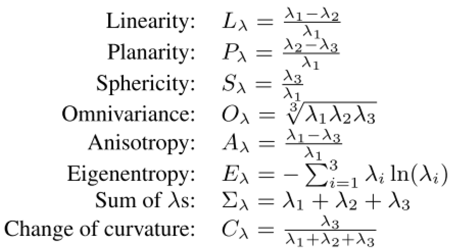
The following covariance features were employed for the processing of vaihingen: R, G, B, Intensity Roughness (r = 1.5 m), Number of neighbors (r = 1.5 m), Omnivariance (r = 1.5 m), Surface variation (r = 1.5 m), Verticality (r = 1.5 m), Surface variation (r = 2 m), Number of neighbors (r = 2 m), Verticality (r = 2 m), Verticality (r = 2.5 m), and the height below 1m with respect to the lowest point within a cylinder of 10 m.

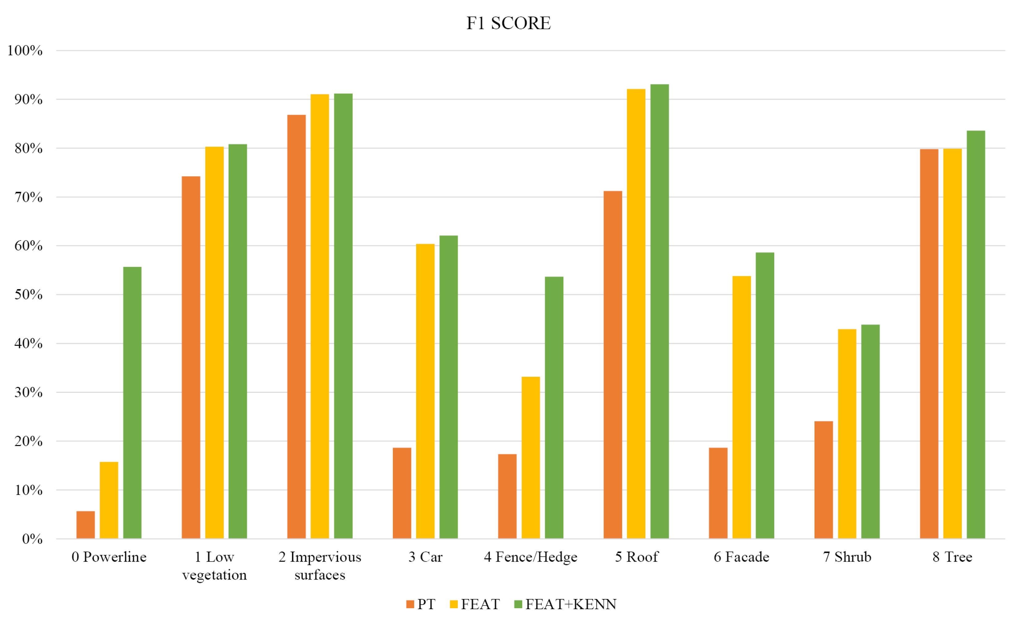
In

Table 3. Class statistics and F1 scores of the ISPRS Vaihingen dataset [20].

	Powerline	Low Veg	Imp Surf	Car	Fence	Roof	Facade	Shrub	Tree	mF1
	Class distribution (%)
	0.1	24.0	25.7	0.6	1.6	20.2	3.6	6.3	17.9
	F1 Score (%)
PT	5.6	74.2	86.8	18.6	17.3	71.2	18.6	24.1	79.8	44.0
FEAT	15.7	80.3	91.0	60.4	33.2	92.1	53.8	42.9	79.9	61.6
FEAT + KENN	55.7	80.8	91.2	62.1	53.7	93.1	58.6	43.8	83.6	68.6

, the F1 scores per class reached with the three previously introduced approaches are reported (also graphically summarized in Figure 8), as are the Overall Accuracy (OA) and mean F1 Score (mF1). As shown, the baseline configuration (PT) achieves quite low levels of accuracy, in particular for the unbalanced classes. The introduction of features (FEAT configuration) allows to raise the “car” F1 score from 18% to 60% for the “cable” class, it goes from a 5% to a still poor 15% F1 score. Overall, the mF1 score increased from the 44.0% baseline to 61.6% with the feature inclusion.

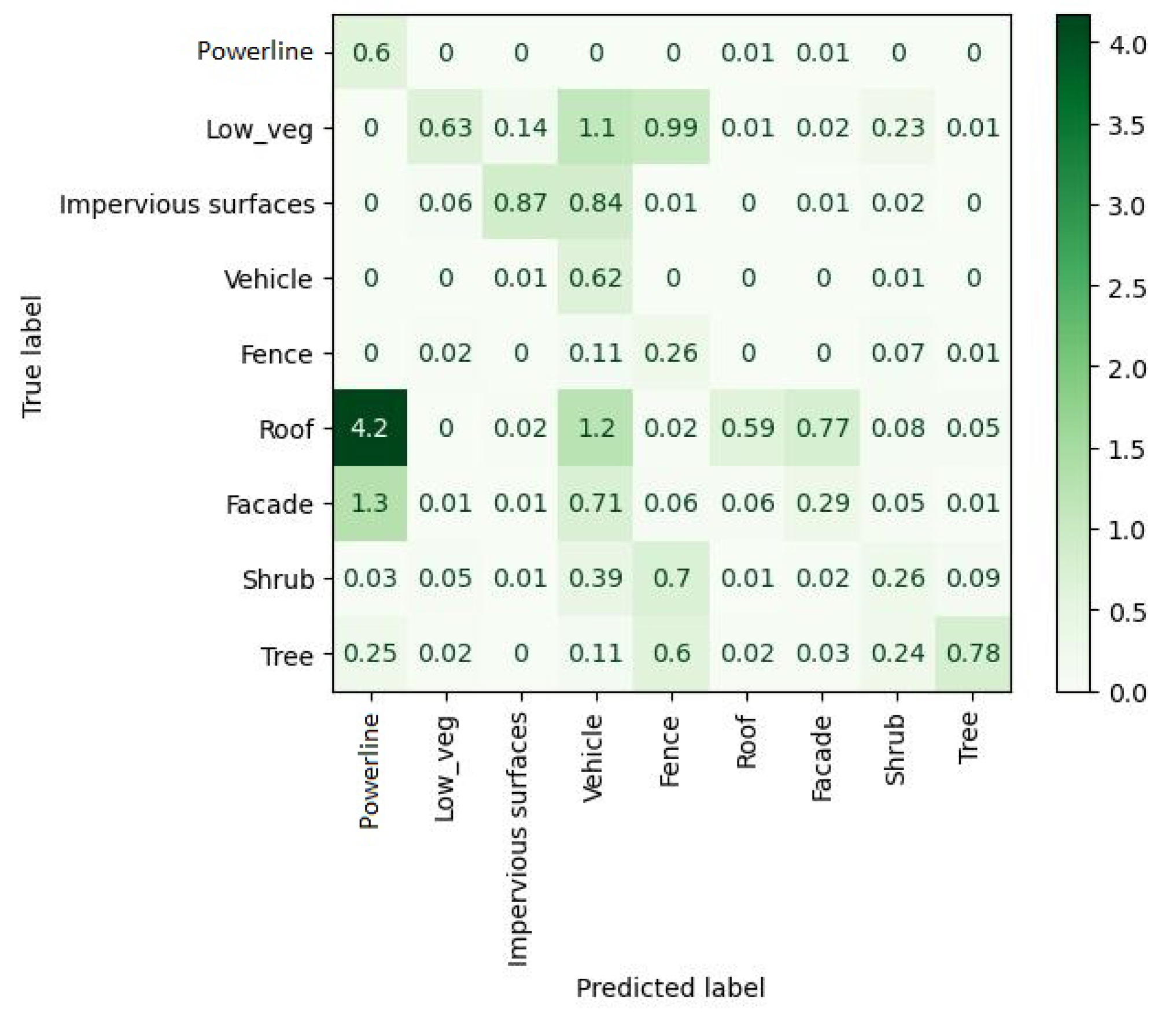
Through an accurate analysis of the confusion matrix extracted for the FEAT configuration (Figure 9), it is possible to understand that most of the points belonging to the class “powerline” are actually predicted as “roof”.

Therefore, in order to intervene and correct such a problem, three types of rules, related to the classes “powerline” and “roof”, have been introduced:

$$\left\{\begin{array}{c}\forall u.\neg The\_highest\left(u\right)\vee \neg Few\_Neighbours\left(u\right)\vee Powerline\left(u\right)\hfill \\ \forall u.Few\_Neighbours\left(u\right)\vee Roof\left(u\right)\hfill \\ \forall u,v.\neg Near(u,v)\vee \neg Powerline\left(u\right)\vee \neg Roof\left(v\right)\hfill \end{array}\right.$$

(9)

In the first two rules, we state that points belonging to the class “powerline” are among the highest points of the dataset and, contrary to the “roof” points, have a reduced number of neighbors. This type of rule works, in particular, in relation to two of the hand-crafted features that have been defined for the dataset: height_below and number_of_neighbours. Height_below considers the difference in the height of each point in a certain neighborhood, while number_of_neighbours the number of points in a fixed radius. Finally, the third rule specifies that points belonging to the classes “roof” and “cable” should be far from each other. The threshold near for this case study has been set to 0.8 m, equal to the double of the point cloud resolution.

The “fence” class also had particularly low accuracy outcomes. The confusion matrix showed that points belonging to this class were, in general, misclassified as “shrub”, “tree”, and “vegetation”. For this reason, the following two rules have been introduced:

$$\left\{\begin{array}{c}\forall u.\neg Short\left(u\right)\vee \neg Noisy\left(u\right)\vee Shrub\left(u\right)\hfill \\ \forall u.\neg Short\left(u\right)\vee \neg Noisy\left(u\right)\vee \neg Fence\left(u\right)\hfill \end{array}\right.$$

(10)

They state that elements that are short and have a high degree of roughness (local noise) have a high probability of belonging to the class “shrub” (first rule) and not “fence” (second rule). Looking again at Table 3 and Figure 8, we can see that the introduction of logic rules was particularly effective for the classes “powerline” and “fence”.

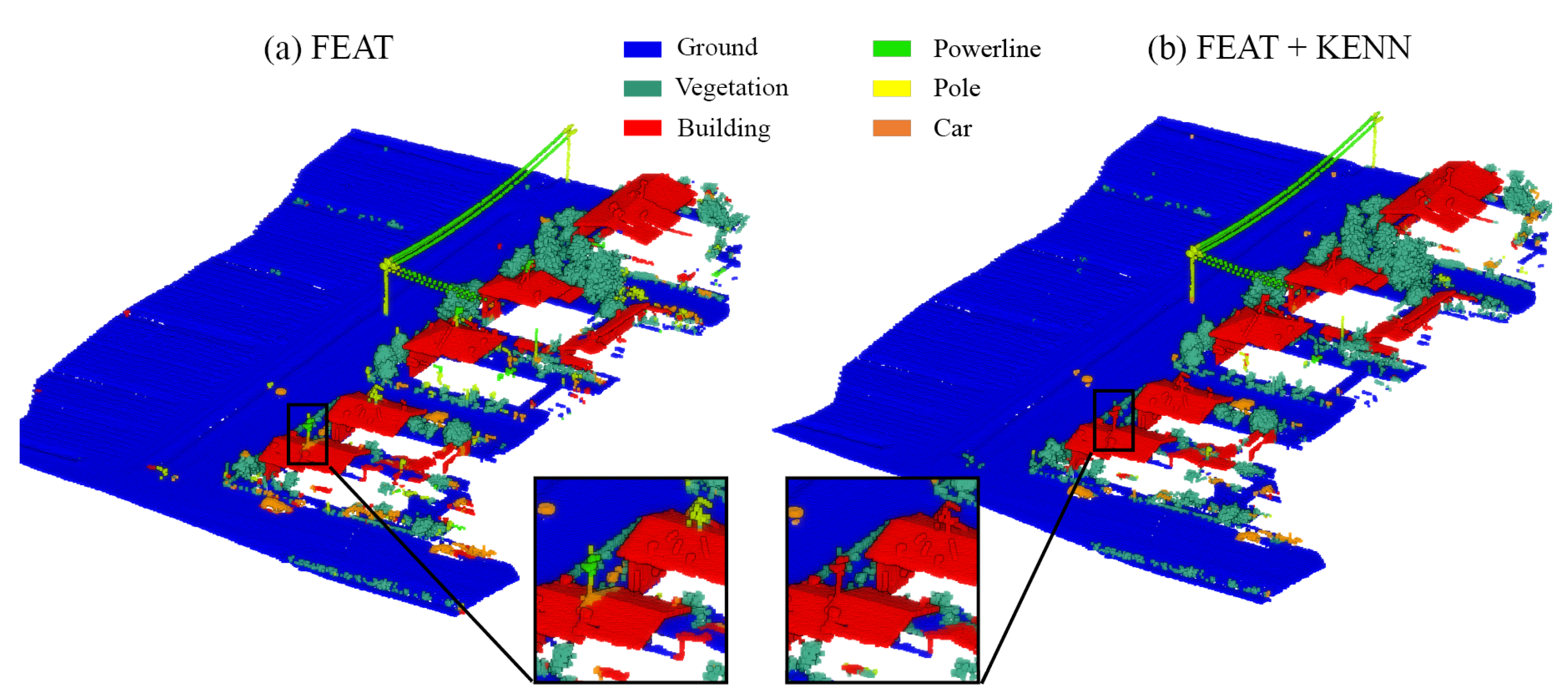
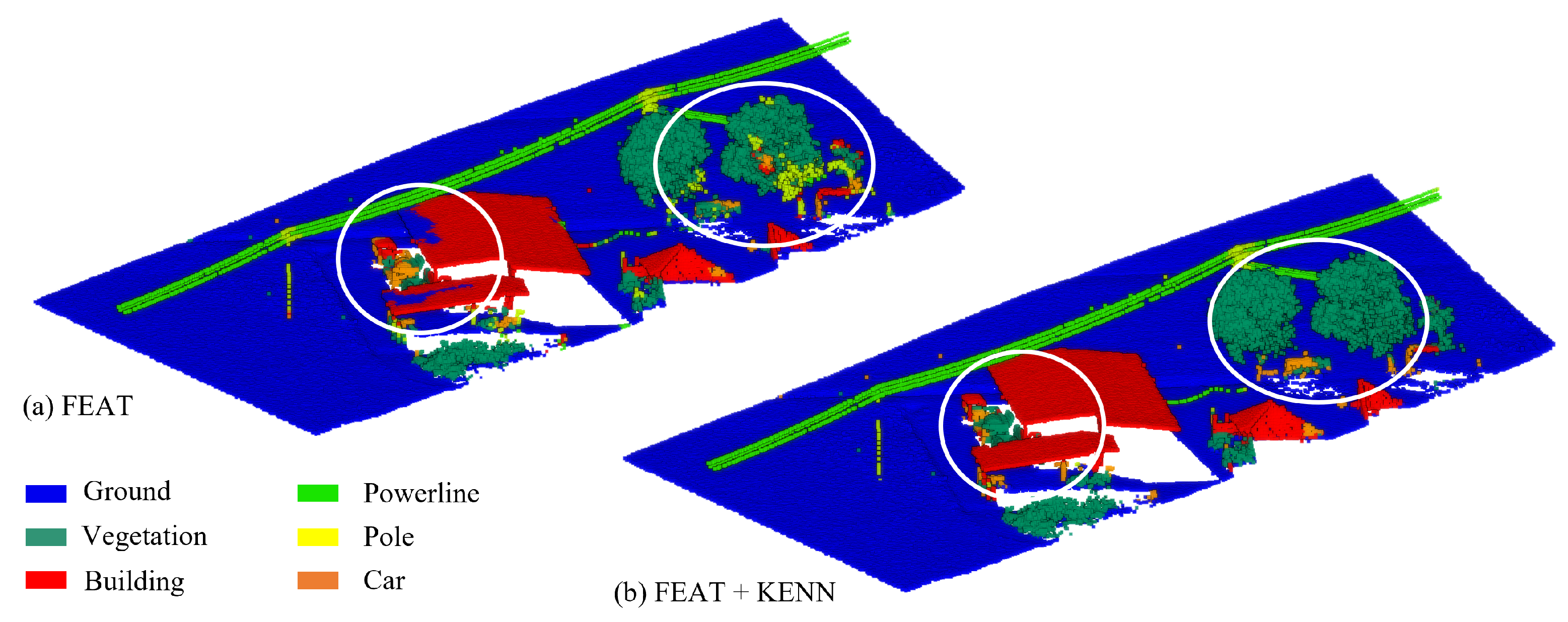
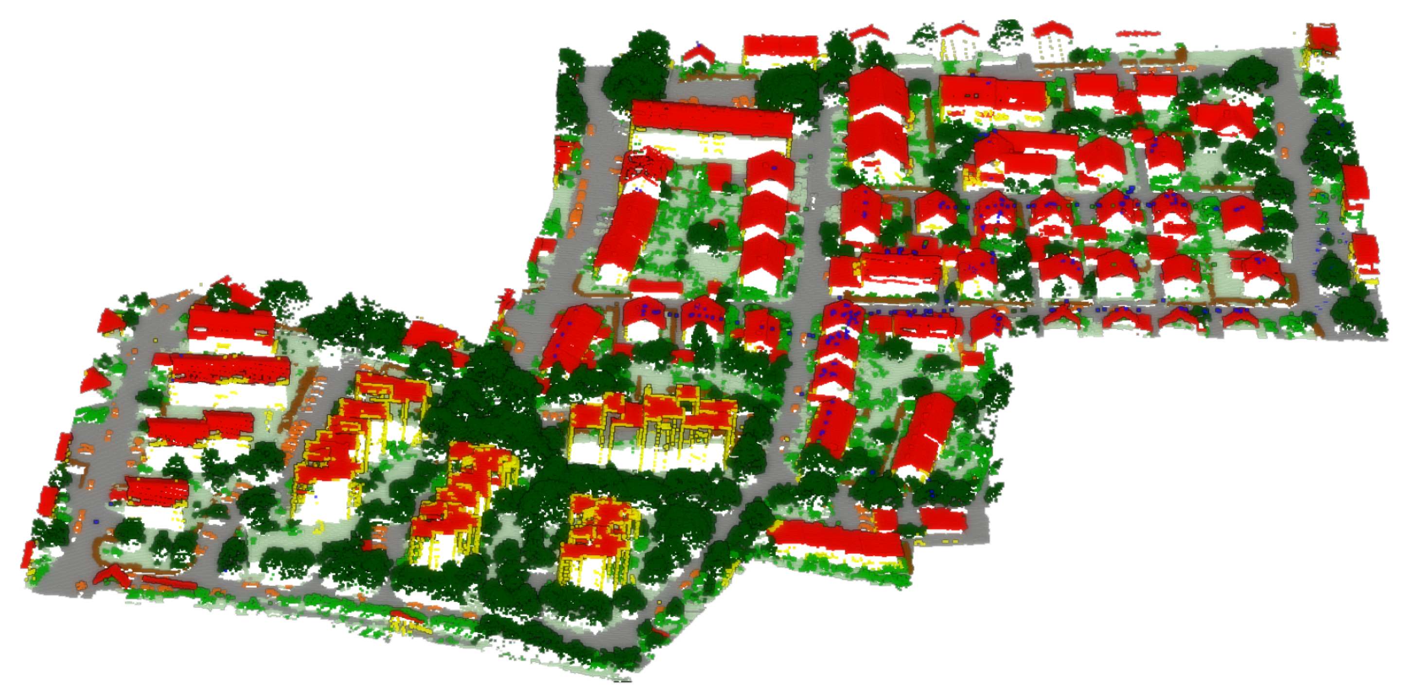
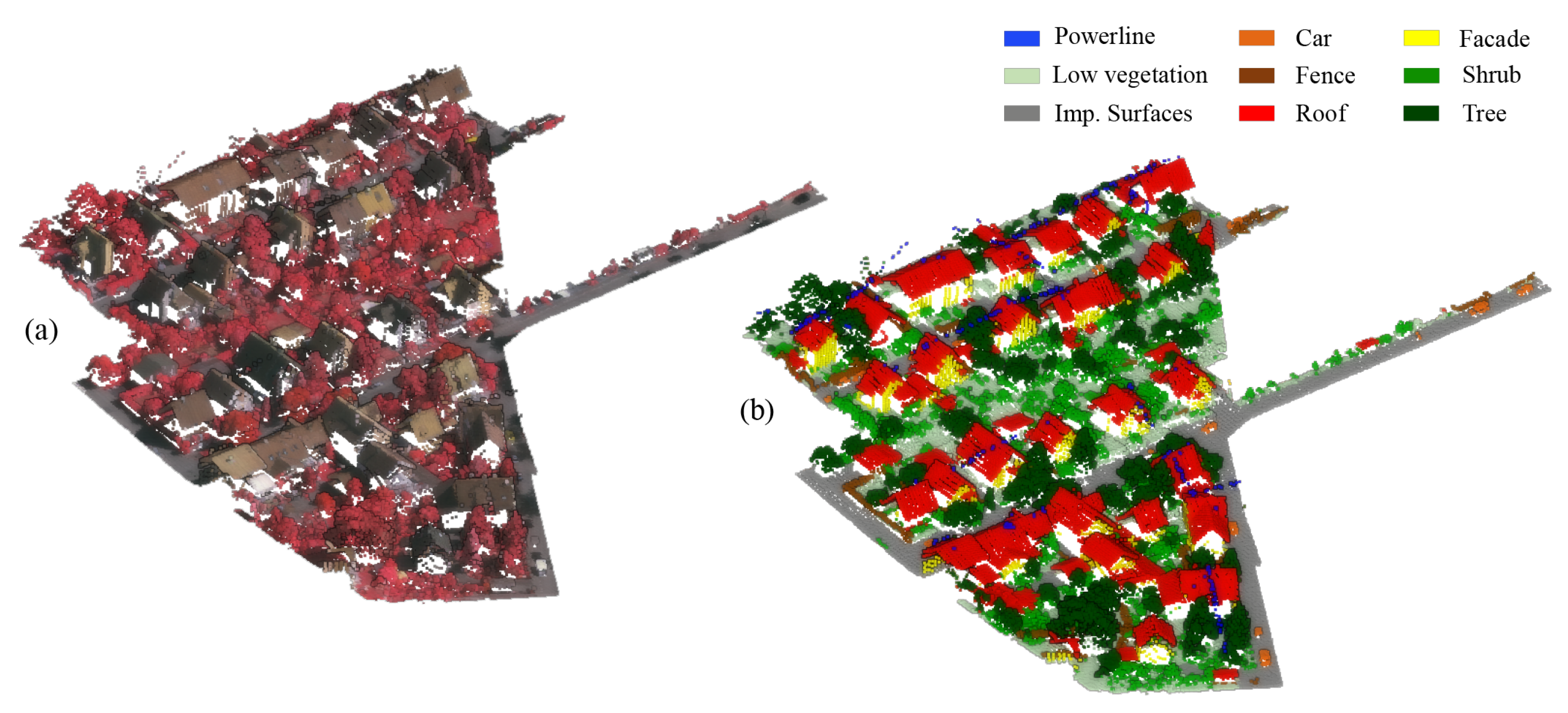
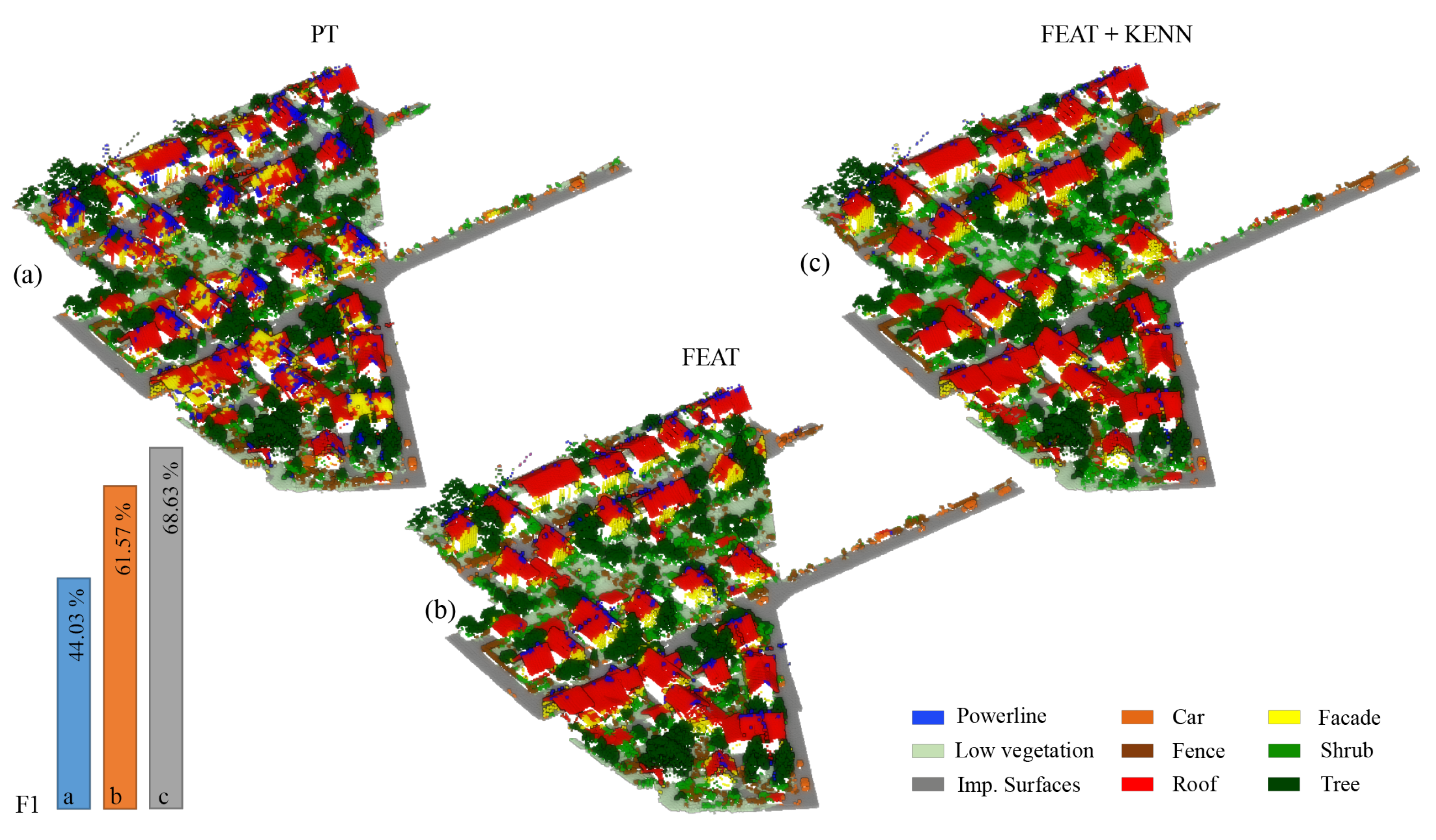
For an overall qualitative evaluation, the manually annotated test dataset (Figure 10) can be compared with the ones semantically segmented using PT, PT plus hand-crafted features (FEAT), and PT plus features and logic rules (FEAT + KENN) (Figure 11). Overall, the mF1 score increased from the 61.57% baseline to 68.63% with the inclusion of a-posteriori knowledge.

Finally, in

Table 4. State-of-the-art results for the Vaihingen benchmark as of April 2023 [61].

	F1 Score (%)
Method	Pow	Low Veg	Imperv Surf	Car	Fence	Roof	Facade	Shrub	Tree	OA	mF1
DGCNN	44.6	71.2	81.8	42	11.8	93.8	64.3	46.4	81.7	78.3	59.7
PointConv	65.5	79.9	88.5	72.1	25	90.5	54.2	45.6	75.8	79.6	66.3
PointNet	57.9	79.6	90.6	66.1	31.5	91.6	54.3	41.6	77	81.2	65.6
RandLA-Net	68.8	82.1	91.3	76.6	43.8	91.1	61.9	45.2	77.4	82.1	70.9
RFFSNet	75.5	80	90.5	78.5	45.5	92.7	57.9	48.3	75.7	82.1	71.6
PointSIFT	55.7	80.7	90.9	77.8	30.5	92.5	56.9	44.4	79.6	82.2	67.7
GANet	65.6	83.3	90.6	77.1	41.6	93.4	61.1	46.9	80.3	82.9	71.1
SCFNet	64.2	81.5	90.8	73.9	35.2	93.6	61.5	43.4	82.6	83.2	69.8
PointCNN	61.5	82.7	91.8	75.8	35.9	92.7	57.8	49.1	78.1	83.3	69.5
KPConv	63.1	82.3	91.4	72.5	25.2	94.4	60.3	44.9	81.2	83.7	68.4
Our	55.7	80.8	91.2	62.1	53.7	93.1	58.6	43.8	83.6	82.7	68.6

, the results achieved with our KENN approach are reported in comparison with other state-of-the-art approaches. It can be seen that there is currently no network predominant over the others and that the proposed KENN method achieves results that are generally in line with the state of the art.

4.2. Hessigheim 3D

The Hessigheim 3D dataset proposed by the University of Stuttgart as an evolution of the Vaihingen dataset serves as a standard in the task of urban-level 3D semantic segmentation. The Hessigheim dataset [3] is high-density LiDAR data of ca 800 points/m², enhanced with RGB colors from onboard cameras (GSD of ca 2–3 cm). The dataset is divided into 11 categories: “Low Vegetation,” “Impervious Surface,” “Vehicle,” “Urban Furniture,” “Roof,” “Facade,” “Shrub,” “Tree,” “Soil/Gravel,” “Vertical Surface,” and “Chimney”. Hessingheim, similar to the Vaihingen dataset, contains several unbalanced classes that are challenging to spot, i.e., “car” and “chimney” (Figure 12 and Figure 13).

The following covariance features were employed for the processing of vaihingen: R, G, B, Reflectance, Verticality (r = 1 m), Linearity (r = 1 m), Number of neighbors (r = 1 m), Roughness (r = 1 m), and again the height below 1m with respect to the lowest point within a cylinder of 10 m.

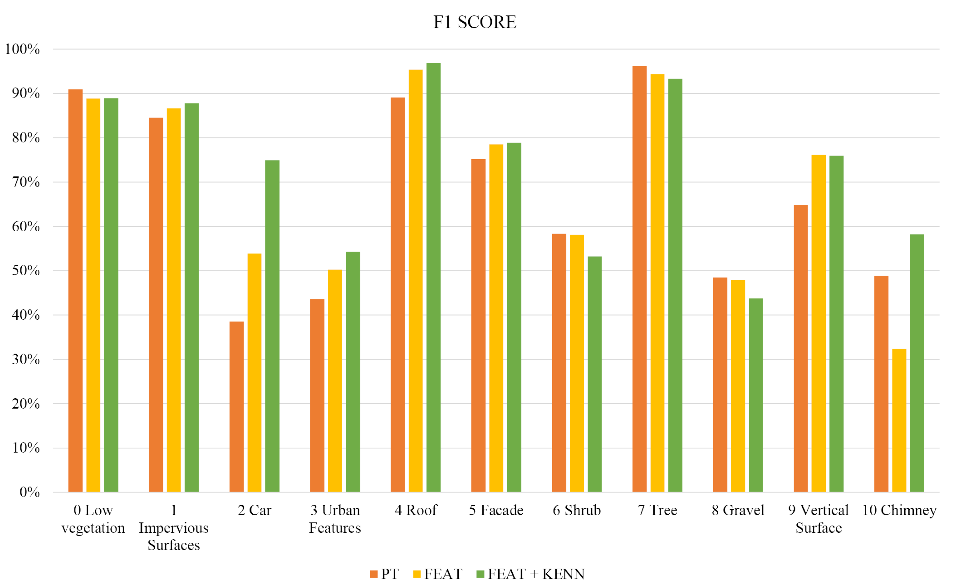
The results achieved with the three different experiment configurations are reported in

Table 5. Class statistics and F1 scores of the Hessigheim dataset.

	Low Veg	Imp Surf	Car	Urb Feat	Roof	Facade	Shrub	Tree	Gravel	Vert Surf	Chimney	mF1
	Class distribution (%)
	36.0	17.5	0.4	1.9	10.6	2.0	1.8	13.6	14.5	1.6	0.1
	F1 Score (%)
PT	90.9	84.5	38.5	43.5	89.6	75.2	58.3	96.2	48.5	64.8	48.9	67.1
FEAT	88.9	86.6	53.9	50.2	95.3	78.5	58.1	94.4	47.8	76.2	32.4	69.3
FEAT + KENN	88.9	87.7	74.9	54.3	96.8	78.9	53.2	93.3	43.7	75.9	58.2	73.3

. As shown, there has been a general improvement in the metrics thanks to the introduction of logic rules, in particular for those under-represented classes of the training data. Overall, the mF1 score slightly improved between the baseline (67.1%) and the feature inclusion (69.3%).

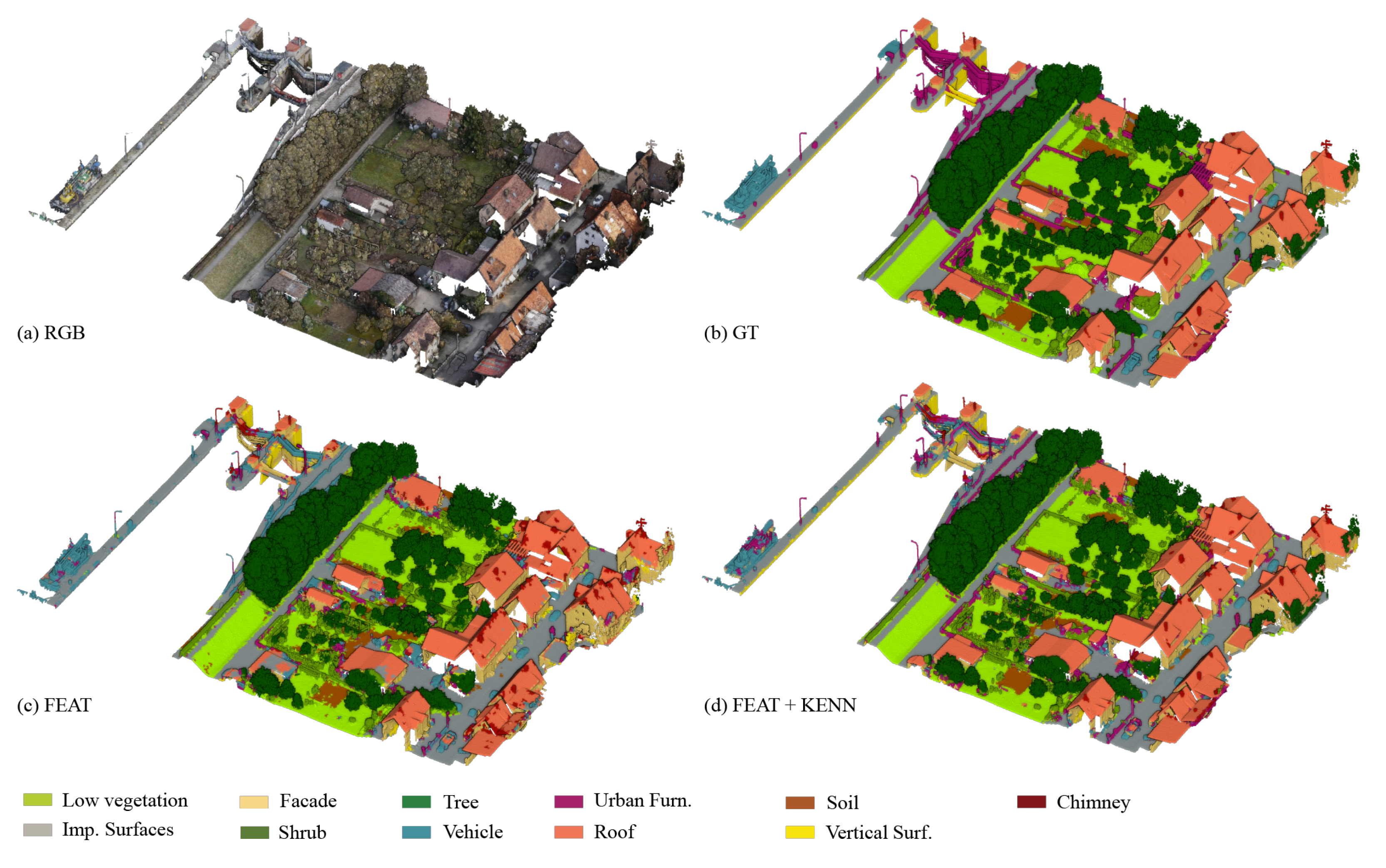
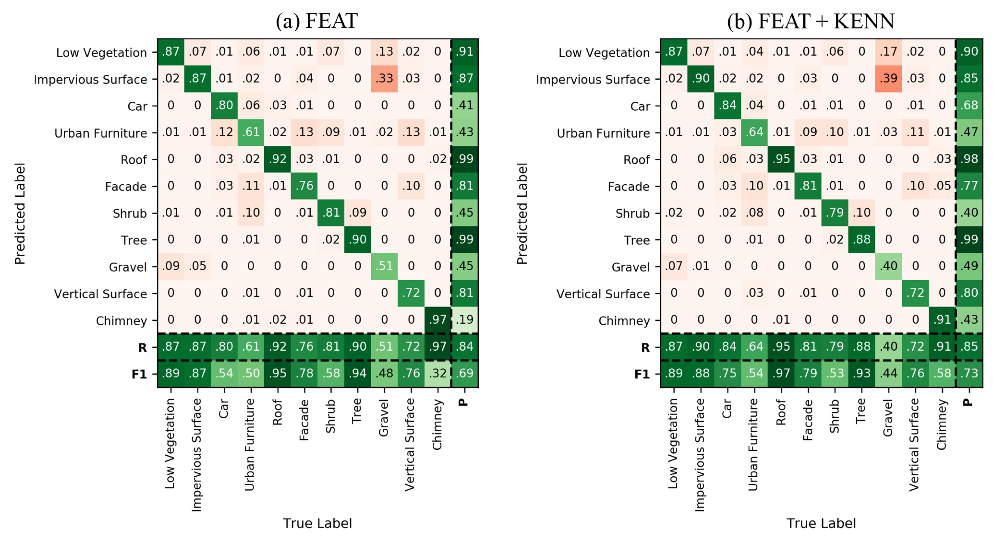
If we have a close look at Figure 14, where the results achieved for the validation dataset are compared with the ground truth, we can see that the FEAT configuration output has two main categories of issues (Figure 14c). First, different fences belonging to urban furniture (purple color) were erroneously predicted as vehicles (light blue color). Second, the majority of the roof’s ridges were identified as chimneys.

The adoption of specific rules for the vehicle and chimney classes led to the solution of these types of issues in the configuration FEAT + KENN (Figure 14d). As regards the car class, the following binary predicates were added:

$$\left\{\begin{array}{c}\forall u,v.\neg Near(u,v)\vee \neg Vehicle\left(u\right)\vee Vehicle\left(v\right)\vee Impervious\_surface\left(v\right)\hfill \\ \forall u,v.\neg Near(u,v)\vee \neg Vehicle\left(u\right)\vee \neg Urban\_furniture\left(v\right)\hfill \end{array}\right.$$

(11)

The above rules state that points of the vehicle class are likely to be close to either other points of the same class or points of impervious surfaces, but not points of the urban furniture class. Given the high density of the point cloud, the “Near” measure for this dataset was fixed to 0.15 m.

Additionally, we described the vehicle as “vertical” and “short” with the following unary statement, reading these values through the previously selected features Verticality and Distance from ground.

$$\left\{\begin{array}{c}\forall u.\neg Vertical\left(u\right)\vee \neg Vehicle\left(u\right)\hfill \\ \forall u.Short\left(u\right)\vee \neg Vehicle\left(u\right)\hfill \end{array}\right.$$

(12)

Two binary rules were established for the class “chimney”: points with a high level of Verticality are assumed to belong to the “chimney” class, while points with a low level of Verticality are expected to belong to the “roof” class.

$$\left\{\begin{array}{c}\forall u,v.\neg Near(u,v)\vee \neg Chimney\left(u\right)\vee \neg Vertical\left(v\right)\vee Chimney\left(v\right)\hfill \\ \forall u,v.\neg Near(u,v)\vee \neg Chimney\left(u\right)\vee Vertical\left(v\right)\vee Roof\left(v\right)\hfill \end{array}\right.$$

(13)

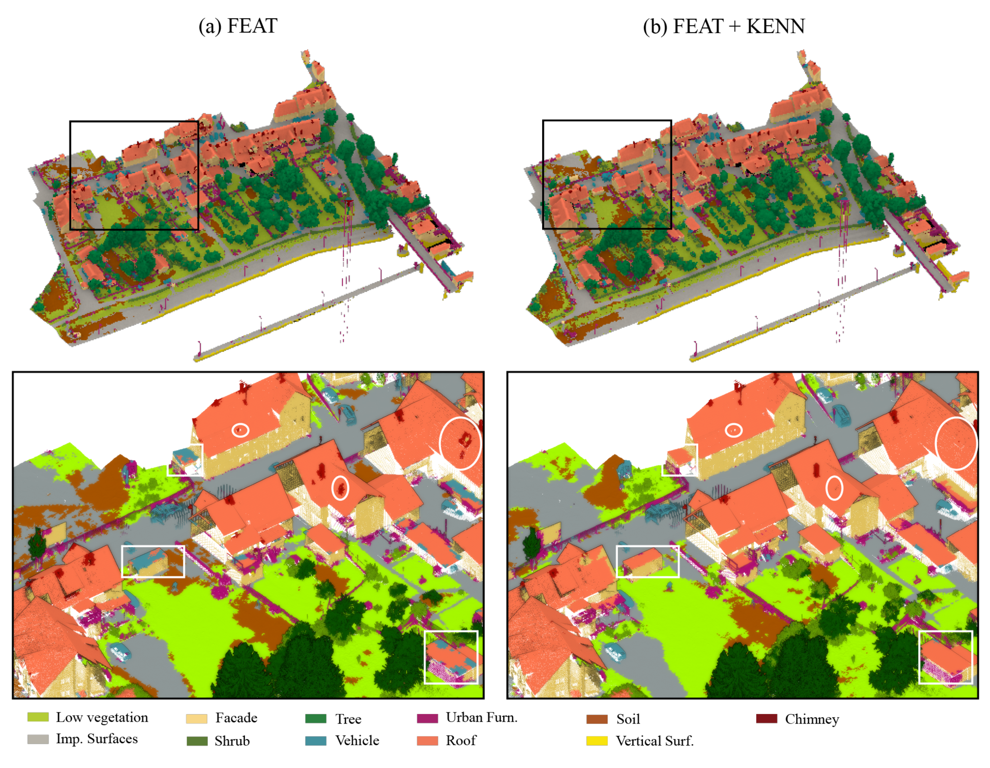
The graphical (Figure 15) and numerical (Figure 16) results achieved with and without the logic rules are compared below. Overall, the mF1 score increased from the 84.41% baseline to 85.33% with the inclusion of a-posteriori rules.

Finally,

Table 6. State-of-the-art results for the Hessigheim benchmark as of April 2023 [62].

Method	Low Veg	Imp Surf	Vehicle	Urb Furn	Roof	Facade	Shrub	Tree	Gravel	Vert Surf	Chimney	OA	mF1
Zhan	58.74	22.06	0.32	16.65	57.06	30.02	5.07	69.34	0.11	28.59	2.22	26.38	46.10
jiabin	66.21	18.02	34.18	38.03	72.00	68.99	47.70	78.65	9.84	35.93	8.32	43.44	58.29
GaoPN++	78.11	72.07	31.78	13.65	73.98	47.79	28.34	71.80	9.65	21.67	4.39	41.20	68.50
Sevgen	83.86	77.21	66.95	42.64	95.60	80.09	59.53	96.06	25.68	81.51	73.85	71.18	79.25
Zhan	84.33	77.86	58.11	42.32	93.25	65.41	53.53	95.29	23.66	59.85	64.66	65.30	79.69
Shi	87.62	85.62	52.40	36.71	95.48	69.30	47.39	94.28	25.08	65.94	38.59	63.49	84.20
ifpRF	90.36	88.55	66.89	51.55	96.06	78.47	67.25	95.91	47.91	59.73	80.65	74.85	87.43
Sevgen	90.88	89.40	77.28	55.76	97.05	81.88	62.06	97.10	23.17	80.27	80.28	75.92	87.59
KPConv	88.57	88.93	82.10	63.89	97.13	85.13	75.24	97.38	42.68	80.87	0.00	72.90	87.69
ifpSCN	92.31	88.14	63.51	57.17	96.86	83.19	68.59	96.98	44.81	78.20	73.61	76.67	88.42
WHU	92.90	90.23	78.51	57.89	95.71	80.43	68.46	97.21	62.37	73.08	72.45	79.02	89.75
Our	88.91	87.74	74.89	54.27	96.83	78.85	53.21	93.28	43.73	75.89	58.22	73.26	85.33

reports a comparison of our results with the state-of-the-art as presented in the Hessigheim portal.

4.3. S3DIS

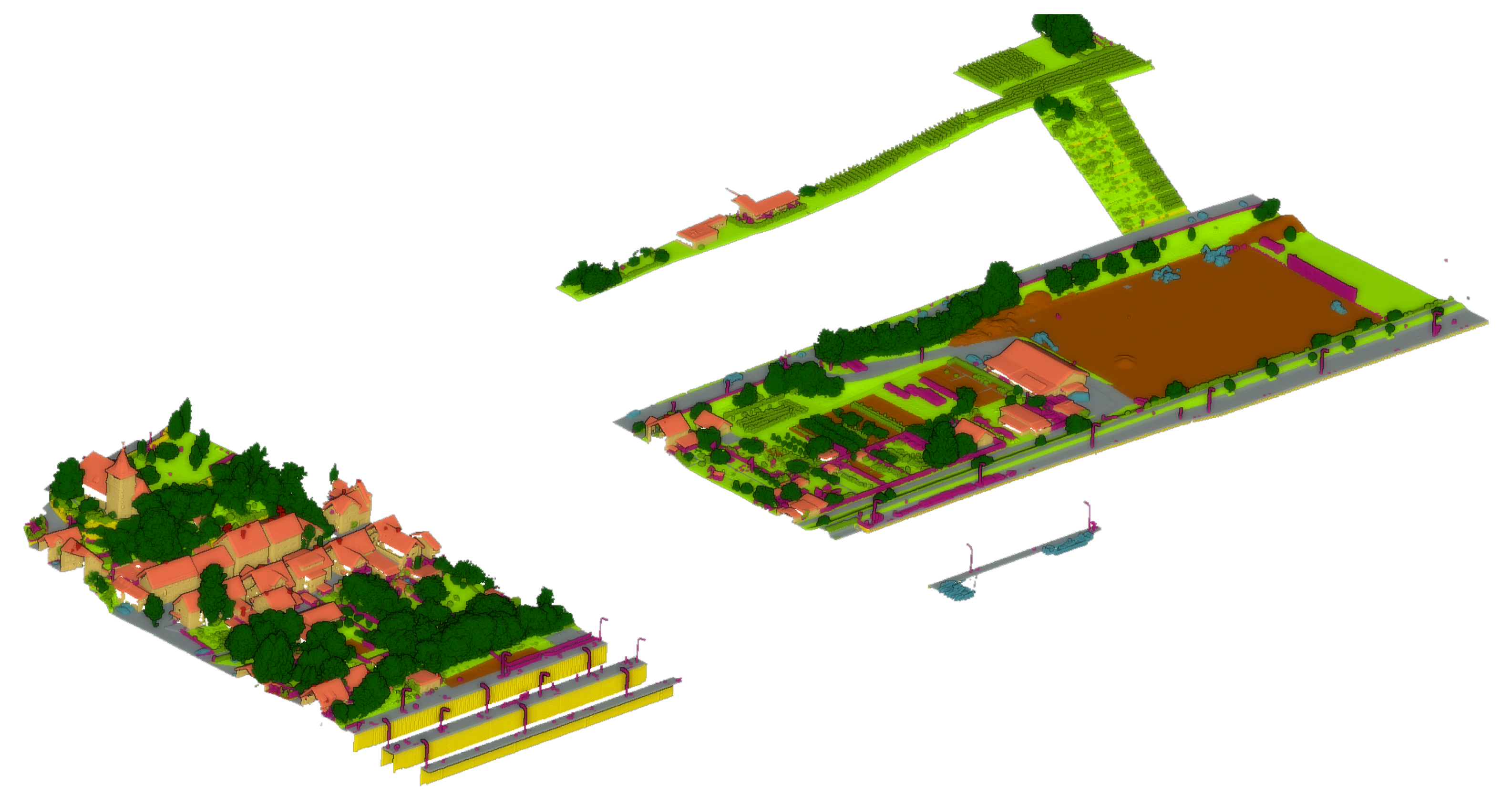
The S3DIS [26] dataset for semantic scene parsing consists of 271 rooms in six areas from three different buildings (Figure 17). Each point in the scan is assigned a semantic label from 13 categories (ceiling, floor, table, etc.). The common protocol is to withhold Area 5 during training and use it during testing, or perform a cross-validation on Area 5. The evaluation metrics include mean classwise intersection over union (mIoU), mean of classwise accuracy (mAcc), and overall pointwise accuracy (OA). As of February 2023, the baseline Point Transformer is 9th in place of the S3DIS benchmark dataset and has been overtaken in recent months by significantly larger networks. However, this study on the relevance of knowledge infusion in Neural Networks is still highly relevant, as knowledge infusion can also be embedded in the newer networks. Moreover, class imbalance and the number of training samples remain a key issue in the S3DIS benchmark (

Table 7. Class statistics and IuO scores of the S3DIS dataset [26]: original benchmark results of Point Transformer and RandLa-net and (top) combined Area 5 results for Point Transformer + Feat + Kenn (bottom).

	Ceiling	Floor	Wall	Column	Beam	Window	Door	Table	Chair	Bookcase	Sofa	Board	Clutter	mIuO
	Class distribution (%)
	19.56	16.54	29.2	1.76	0.03	3.52	3.03	3.75	1.87	10.35	0.3	1.18	8.92
	IuO (%)
PT	94.0	98.5	86.3	0.0	38.0	63.4	74.3	89.1	82.4	74.3	80.2	76.0	59.3	70.4
RandLA-Net	92.7	95.6	79.2	61.7	47.0	63.1	67.7	68.9	74.2	55.3	63.4	63.0	58.7	68.5
PT (combined)	87.3	90.8	49.5	11.7	11.4	55.8	29.9	54.9	43.9	54.7	38.1	34.4	35.6	46.0
FEAT	89.8	91.9	60.1	19.5	28.3	60.4	40.0	57.1	53.1	58.1	33.3	41.5	42.6	52.0
FEAT + KENN	95.5	97.7	64.5	20.8	26.5	69.3	49.3	66.7	67.6	63.0	57.1	50.1	50.3	59.9

). The ceiling, floor, and wall classes are overly dominant with on average nearly 65% of the points and thus also achieve the highest detection rate (respectively 94.0%, 98.5%, 86.3% IoU on the baseline Point Transformer). S3DIS clearly shows that classes with percentual less training data, such as windows (3% of the data, 63.4% IoU) and doors (3% of the data, 74.3% IoU), have a significant drop in performance. Poor class delineations, as with the beams (38% IoU), remain unsolved.

Additionally, there is a significant catch to these fairly good detection rates. The base PointTansformer and even RandLA-Net [33] network only achieve near 70% mIuO on the separated rooms of S3DIS, which is the original training data. When the rooms are combined into one region, which would be the case for a realistic project, the detection rates plummet. Point Tansformer barely achieves 46% mIuO, and so does RandLA-Net with 35% mIuO. Nearly all classes suffer from increased complexity from a room-based segmentation to an area-wide segmentation, except for some classes that already performed poorly with the conventional training data (Table 7 first row).

Analogous to the above two datasets, the prior knowledge aims to improve performance on subideal training data, i.e., on the combined cross-validation of Area 5. The initial RandLA-Net and Point Transformer baselines indicated significant underperformance in all but the ceiling and floor classes. Therefore, we use the a-priori knowledge to generate distinct signatures for all the other classes. For S3DIS, the following features were introduced based on the inspection of the baseline classification: R, G, B, Planarity (r = 0.2 m), Verticallity (r = 0.5 m), Surface variation (r = 0.1 m), Sum of Eigenvalues (r = 0.1 m), Omnivariance (r = 0.05 m), Eigenentropy (r = 0.02 m), and the normalized Z value. The verticality and planarity help identify the more planar objects in the scene, such as tables, doors, and bookcases. In contrast, the Eigenentropy, Omnivariance, Surface variation, and Sum of Eigenvalues at different radii help describe the curvature of table, chair, and sofa elements.

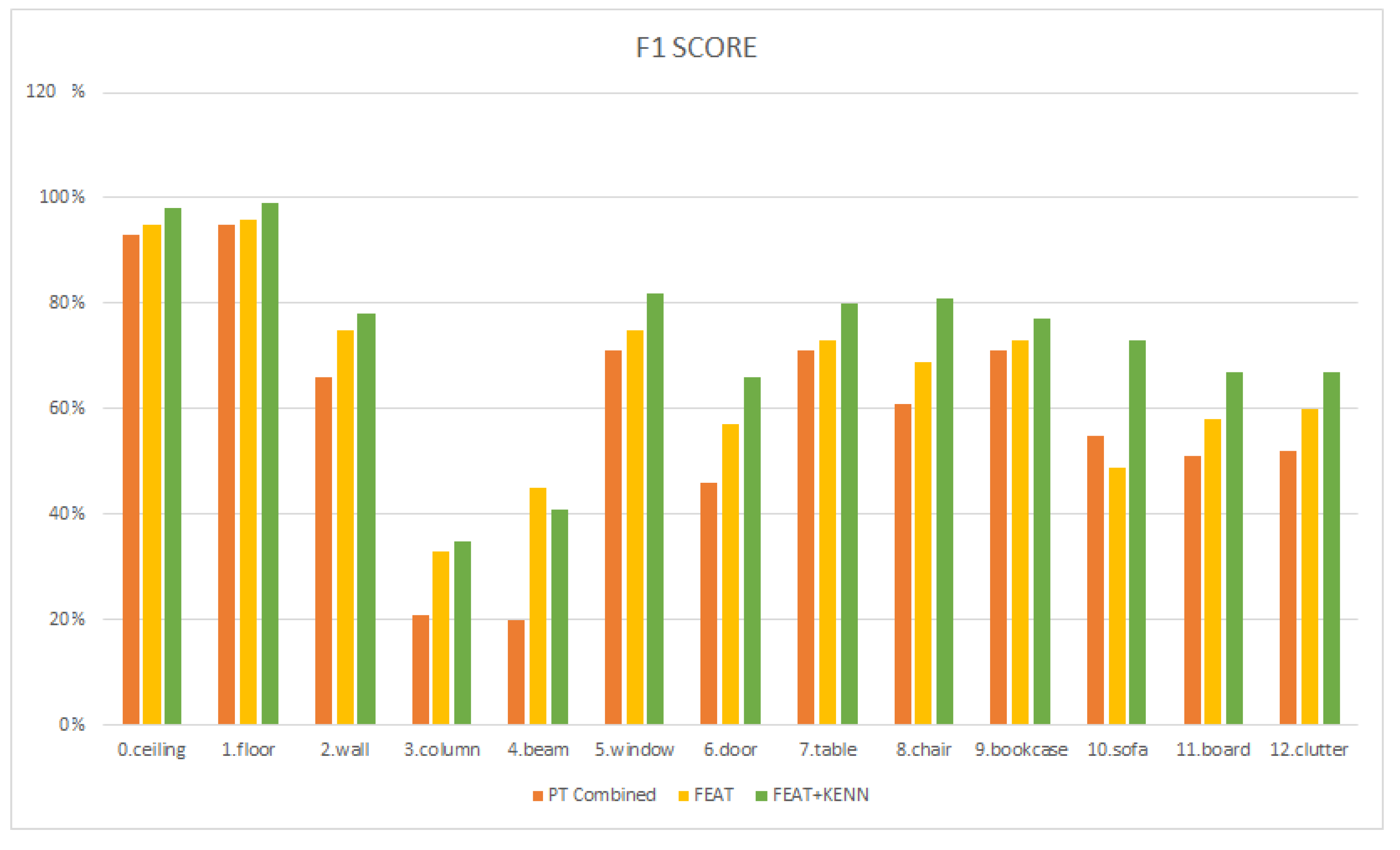
The results achieved with the a-priori knowledge are reported in Table 7 line 3 and Figure 18. There is a significant improvement in nearly all classes but sofa, with an overall increase in 6% mIuO. The best improvements are reported for the walls (10.5%), beams (17.0%), doors (10.0%), and chairs (9.1%), which now show significantly less confusion with clutter and with overlapping classes in the case of the walls (Figure 19).

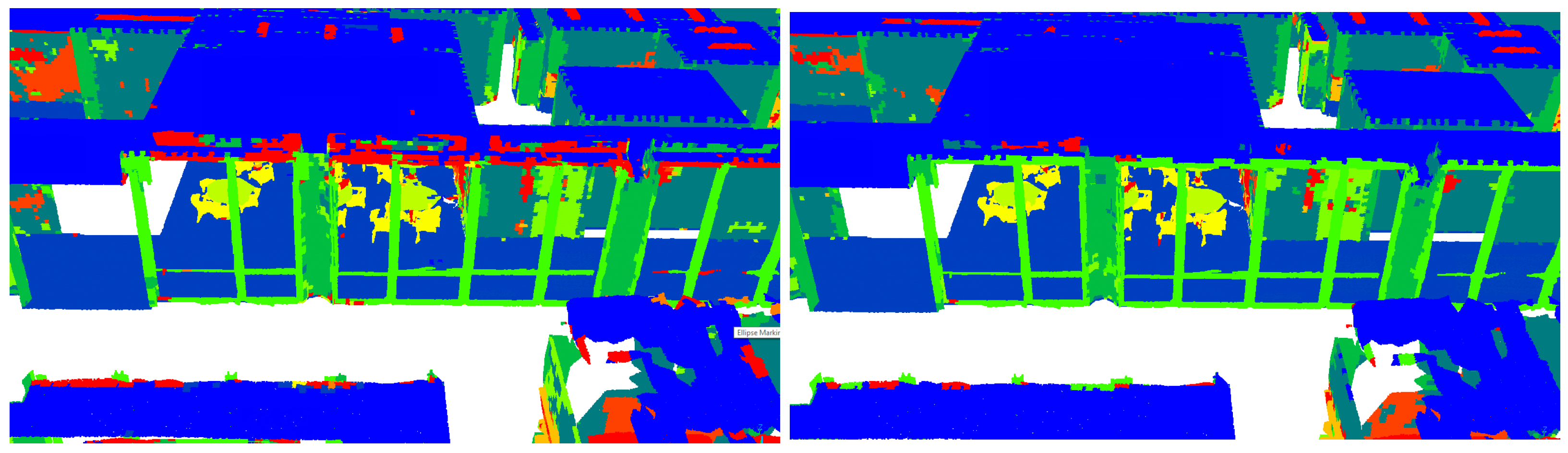
Despite the improvements, two key categories of confusion are identified (Figure 20). First, there are a significant number of false negatives within the classes, despite the observations being surrounded by a large number of points attributed to a single class. Second, there is significant confusion between wall-based elements such as windows, doors, bookcases and the walls themselves. This is a known problem and remains a difficult obstacle for state-of-the-art networks.

The a-posteriori rules specifically target these two issues using binary rules. First, class consistency is forced between the classes using nearby class-associativity, e.g.,

$$\forall u,v.\neg Near(u,v)\vee \neg wall\left(u\right)\vee wall\left(v\right)$$

(14)

where each class is incentivized to enforce class consistency at nearby points. Specifically for classes with a descent surface area, i.e., walls, windows, and doors, this is quite promising. Second, the expected topology can be formulated as ’Near’ rules to lower the confusion between neighboring classes, e.g.,

$$\forall u,v.\neg Near(u,v)\vee \neg floor\left(u\right)\vee sofa\left(v\right)\vee chair\left(v\right)\vee table\left(v\right)$$

(15)

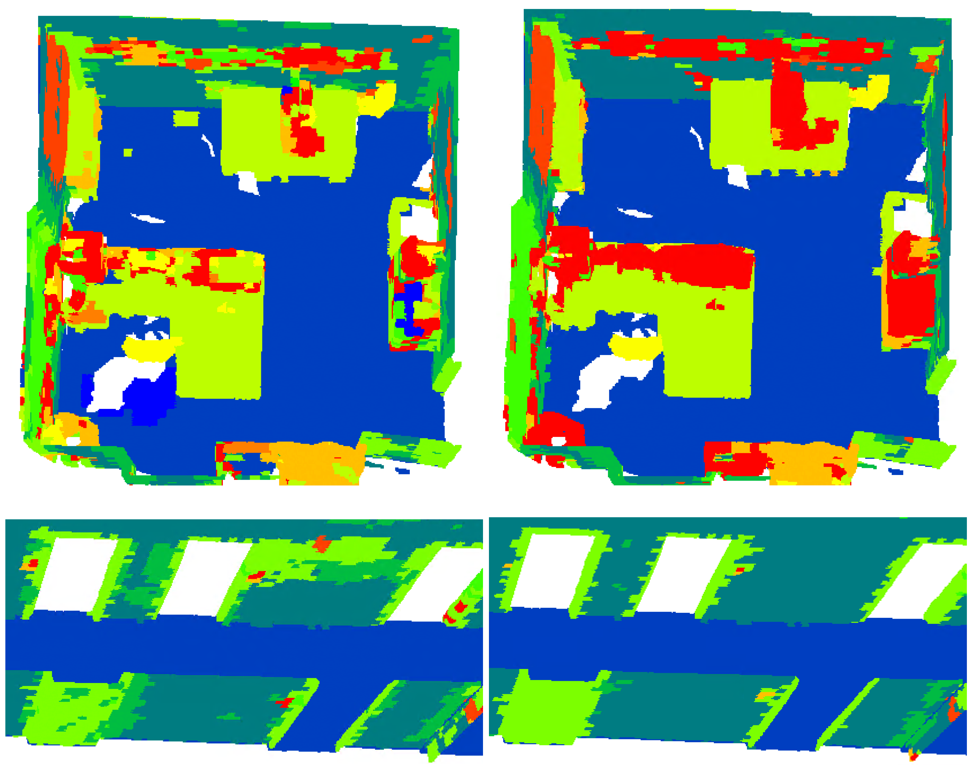
where the promixity of certain classes, i.e., furniture elements near the floor and windows, doors, boards, and columns near walls, is reinforced. Looking again at Table 7 and Figure 18, it is clear that the a-posteriori knowledge again significantly increased the performance from an average mIuO of 52.0% to 59.9% compared with the a-priori knowledge. The highest increase is noted in the sofa (23,8%), chair (14.5%), and table classes (9.5%), which are directly affected by the knowledge infusion. Similarly, the windows (8.9%), doors (9.3%), and walls (4.4%) also improved. Overall, separate training sessions indicated that the associativity knowledge offered a better statistical improvement as many stray points are now assigned to the correct class. In contrast, the topological knowledge remedied more isolated but important miss-classifications (Figure 21).

4.4. Performance Evaluation

In this section, the performance of the three configurations for each test case is jointly discussed. For the experiments, a GPU Nvidia RTX 3080, 32 GB of RAM, and a 11th Gen Intel(R) Core(TM) CPU i7-11700KF @ 3.60 GHz were used. It is observed that the computational time increases with the infusion of knowledge (

Table 8. Comparison of the average computational time per epoch per testcase.

	Vaihingen	Hessigheim	S3DIS
	sec/epoch	sec/epoch	sec/epoch
PT	0.7	8.4	82.1
FEAT	2.6	12.8	97.6
FEAT + KENN	3.3	17.5	136.0

). In the first dataset, the highest time increase is generated by adding the a-priori knowledge to the network, while this is less the case for the later two experiments. This can be partially explained by the number of features that are introduced to each network, i.e., 13 for Vaihingen, 9 for Hessigheim, and 10 for S3DIS. However, a prominent factor is the number of classes. These seem to inversely affect the proportional computational effort needed to train the expanded input layer in comparison to the training of the network itself, which is identical to the base network. A higher number of classes significantly complicates the training of the internal network, and thus networks with more classes (9 for Vaihingen, 11 for Hessigheim, and 13 for S3DIS) will be computationally less affected by an increased number of inputs.

The addition of the KENN layers significantly increases the computational effort of the training. The computational effort is a direct result of the number of rules, the number of KENN layers (3 for all networks), and the number of classes. The training times on average increased for Vaihingen by 30% (20 rules, 9 classes), Hessigheim by 36% (12 rules, 11 classes), and S3DIS by 39% (17 rules, 13 classes). This indicates that the number of classes is again the dominant factor in the increase in the computational effort of the proposed method.

5. Discussion

In this section, the pros and cons of knowledge infusion are discussed. The first major aspect is the specificity of the method. Both the a-priori and a-posteriori knowledge are dataset-specific and need to be adjusted for every project. While this seems against the generalization trend of deep learning approaches, it is in fact no different from all the pre-processing steps that have to be performed in current networks nowadays. Training data gathering, curation, and balancing all require dataset-specific and often manual approaches. Even network architecture performance significantly varies given slightly different datasets, as demonstrated in the S3DIS experiments. As such, KENN is a feature that expands a network’s applicability beyond that of a benchmark. Additionally, the production of rules and features takes little human effort, especially when compared with the production of additional training data.

A second aspect is the generalization potential of KENN. In theory, both the a-priori and a-posteriori knowledge could be standardized and used in all datasets. However, generalizing the features and rules would counteract the specificity with which training data issues must be resolved. Each project has its own issues, so unique rules are an ideal solution. Furthermore, employing too many rules (even general ones) would entangle the inference and make it untraceable what the actual contributions of the rules are. Instead, KENN takes the best of both worlds by implementing general class associativity and then allowing users to employ 5 to 10 rules to remedy training data shortcomings.

A third aspect is the portability of the method to other networks. In theory, any network that uses keras layers as in-and output can be enriched with KENN. However, the internal architecture of the network must be compatible with the expansion of the input layers. At the backend of the network, there are fewer issues since KENN directly takes the network’s outputs as input. However, the knowledge is currently tied to spatial semantic segmentation and would require rework if used for anything other than 3D semantic segmentation.

6. Conclusions

This article proposes a new approach for 3D point cloud semantic segmentation that incorporates knowledge-based rules into a neural network. Overall, our contribution provides a promising solution for addressing some challenges, in particular for unbalanced classes in point cloud semantic segmentation by leveraging the power of logic-based rules to facilitate the identification and labeling of minority classes. Concretely, we expand the inputs of the network using a-priori features, which are also used in conventional machine learning. At the backend of the network, we introduce additional final layers to incorporate background knowledge into the neural network’s learning pipeline. The method is implemented on an existing, performant Point Transformer network, given the excellent performances demonstrated in the literature.

The method is tested on both aerial and urban benchmark datasets, i.e., ISPRS Vaihingen, Hessigheim 3D, and S3DIS. The experiments show that the proposed KENN method can improve the performance of the Point Transformer model. The proposed method performs similarly to other well-established algorithms, and it allows for good metrics in particular for under-represented classes. Additionally, KENN succeeds in reducing systematic false positives that are difficult to detect in the training statistics. The rules can be customized based on the scenarios and intuitively created by the user. Furthermore, KENN can potentially be adapted for any 3D semantic segmentation network.

In future work, we intend to integrate KENN with additional neural networks and test the proposed approach in other scenarios (e.g., industry, heritage, etc.). Overall, the presented approach offers additional applicability for existing networks and has the potential to remedy data shortcomings in semantic segmentation training datasets.