Article

Delineating Polynya Area Using Active and Passive Microwave Sensors for the Western Ross Sea Sector of Antarctica

1
School of Geography Environment and Earth Sciences, Victoria University of Wellington, Wellington 6012, New Zealand
2
School of Physical and Chemical Sciences, University of Canterbury, Christchurch 8041, New Zealand
3
Landcare Research, Palmerston North 4474, New Zealand
*
Author to whom correspondence should be addressed.
Remote Sens. 2023, 15(10), 2545; https://doi.org/10.3390/rs15102545
Submission received: 31 March 2023 / Revised: 30 April 2023 / Accepted: 9 May 2023 / Published: 12 May 2023
(This article belongs to the Section Environmental Remote Sensing)

Abstract

:
A polynya is an area of open water or reduced concentration of sea ice surrounded by either concentrated sea ice or land ice. They are often seen as sites of intense ocean–atmosphere heat exchange and as ice production factories. Given their importance, it is crucial to quantify the accuracy of satellite-derived polynya information. Polynyas in their early evolution phase are generally narrow and occur at scales likely too fine to be detected by widely used passive microwave (PMW) radiometric sensors. We derived 40 m scale polynya information over the western Ross Sea from high-resolution Synthetic Aperture Radar (SAR) Sentinel-1 C-band data and examined discrepancies with larger-scale estimates. We utilized two automated algorithms, supervised (a rule-based approach) and unsupervised (a combination of texture analysis with k-means clustering), to accurately identify the polynya areas. We generated data for validation using Sentinel-1 data at instances where polynyas can be visually delineated. Results from PMW sensors (NSIDC and AMSR2) and SAR-based algorithms (rule-based and texture-based) are compared with manually delineated polynya areas obtained through Sentinel-1. Analysis using PMW sensors revealed that NSIDC overestimates larger polynyas and underestimates smaller polynyas compared to AMSR2. We were more accurately able to identify polynya presence and area using Sentinel-1 SAR observations, especially in clear cases and cases when PMW data miscalculates the polynya’s presence. Of our SAR-based algorithms, the rule-based approach was more accurate than the texture-based approach at identifying clear polynyas when validated against manually delineated regions. Altogether, we emphasize the need for finer spatio-temporal resolution data for polynya studies.

1. Introduction

Insight into the distribution of sea ice is crucial to understanding ocean–atmosphere heat exchange and water-mass transformation in Polar Regions and understanding the future trajectory of sea ice in both hemispheres. Of particular interest in this context are polynyas, which are sites of intensive ocean–atmosphere heat exchange during winter, often regarded as ice-production factories. Polynyas are large zones of continual thin ice or open water that often have reduced sea ice concentrations in winter and are enclosed by regions of higher sea ice concentration [1,2]. They can also manifest as recurring elongated areas of open water and thin ice observed [3] along the coastline or the fast-ice edge within the marginal sea ice zones of the polar oceans. They occur at different spatial scales [3], from as large as 105 km2 to as small as 10 km2. A combination of persistent and dynamic factors [4] influence the formation of polynyas. Along the Antarctic coast, there are regions with ice shelves and fast ice, where sea ice is highly sensitive and varying, leading to a complex interplay between ocean and atmosphere processes [5,6]. Based on the mechanisms controlling their formation, polynyas are categorized as either open-ocean or coastal. Open-ocean, or sensible heat, polynyas are formed due to convective ocean currents [7], and usually form in the middle of the ocean, far from coasts or other barriers [2,8,9]. They form when warmer water upwells from deeper oceans to the surface due to ocean bottom topography or overturning. As heat is transferred from this water to the sea ice, it melts, and new ice formation is inhibited.
Coastal, or latent heat, polynyas form when directionally constant offshore winds push the sea ice away from a barrier, such as fast ice, an iceberg, or an ice shelf. Ice production is not inhibited and new sea ice is removed via advection as it forms [10]. Considerable ocean–atmosphere heat flux occurs during this ice formation [11], modulating the global ocean thermohaline circulation [12]. Coastal polynyas alter shelf waters [13], modify mesoscale atmospheric motions [14,15] and are regarded as atmospheric CO2 sinks [16] and areas of huge phytoplankton accumulation [17] and thus play an important role in biogeochemical cycles [18]. Studies [19,19] highlighted the importance of polynyas for insights into ice shelf circulation.
The western Ross Sea is a particularly important region for sea ice formation due to persistent offshore winds that form coastal polynyas [20]. Moreover, the low-saline shelf water and the Modified Circumpolar Deep-Water masses that enter this zone from the north and east of the Amundsen Sea, circulate along the ice shelf and are controlled by freezing, salt rejection, and melting of sea ice. The densest waters in the Ross Sea form in the west when the winter freezing and salt rejection [21,22] begins during sea ice formation. Studies suggest that the most saline part of this dense water, the High Salinity Shelf Water (HSSW), occurs in the latent-heat polynyas of Terra Nova Bay and Ross Sea polynya (between 160 and 180°E) due to high salt fluxes [23] into the ocean associated with continuous sea ice formation.
Passive Microwave Radiometers (PMW) [24,25] have been widely used to estimate polynya areas as they are unaffected by cloud cover and have frequent acquisition rates. However, PMW datasets are also known to under- or over-estimate [7,26,27] low ice-concentration zones. These low ice concentration zones are generally thin-ice regions in winter. There are two ways to detect polynya using PMW data: threshold-based, and the polynya Signature Simulation Method (PSSM) [24,25,28]. The former defines a particular threshold of sea ice concentration fields to define polynya areas, whereas the latter is based on polarization ratios (vertical minus horizontal polarized brightness temperatures divided by their sum) to classify open water and initial stage sea ice types [24]. In their early evolution phase in this region, polynyas are narrow and occur at smaller scales so PMW sensors, given their coarse spatial resolution [3], struggle to identify them [29].
To overcome these limitations, the Arctic Radiation and Turbulence Interaction Study Sea Ice (ASI) algorithm [30,31] was created to identify open water areas more reliably and seems capable of distinguishing between the initial ice types [24] (greasy frazil-ice, a mixture of thin-ice and open water [7]. Nevertheless, ASI also uses PMW as a source which is vulnerable to the presence of meltwater on the ice [31], which is essential for accuracy in thin-ice zones [32,33]. Several studies [3,34,35] demonstrate the need to identify comprehensive spatial information about the deformation processes in these zones. Alternatively, visible sensors [3,7] with meter-scale resolution allow localized analyses of different polynya zones. However, they are not useful during the polar night, and frequent cloud cover also limits their application in this region [36]. The Ross Sea is an important area as it features the largest polynya formation in Antarctica; hence understanding the polynya processes occurring at smaller scales is crucial. In particular, deriving polynya areas with better accuracy [37] is essential to quantifying their role in large-scale processes.
Some of the limitations of optical and passive microwave data can be overcome by Synthetic Aperture Radar (SAR) data, which functions day and night unaffected by cloud cover and obtains imagery at very high spatial resolutions. Several studies have used SAR to separate sea ice types from open water [38,39,40,41,42,43,44,45,46,47,48] to determine the advection of pack ice [49] away from the polynya region and sea ice drift velocities [33]. Dai et al. [38] used Sentinel-1 SAR (S1) data to manually delineate the extent of the Ross Sea polynya between 2017 and 2018. Lei et al. [50] used S1 data to interpret polynya events in Greenland. Lohse et al. [42,43] have also used S1 for mapping sea ice types by considering the surface-type dependent effect of incidence angle on returns. To quantify and evaluate the parameters that best suit sea ice classification, texture analysis [51] was also applied to European Space Agency (ERS-1) SAR data. Altogether, there is increasing literature on using S1 and SAR for sea ice applications [44,45,46,52] in recent years, highlighting its potential.
In this study, we examine the potential of S1 C-band data to identify and separate the polynyas from adjoining pack ice. As polynyas are generally classified as regions of thin ice in winter [27], this study aims only at identifying such thin-ice zones. We examine the potential of two approaches: a rule-based technique, and texture-based analysis combined with a k-means clustering scheme. We generate a quantitative analysis from S1 data and compare it to existing PMW-based polynya areas. In addition, we identify the circumstances where our SAR-based algorithms are more reliable in identifying the coastal polynyas with a finer spatial resolution. We emphasize the need for high-resolution datasets to identify polynyas.

2. Study Area and Materials

2.1. Study Area: The Ross Sea Region

The Ross Sea is situated in the southernmost part of the Pacific Ocean (inset in Figure 1) and interacts with the Antarctic coastline along the Transantarctic Mountains. This region is home to three recurring latent heat polynyas: Ross Sea polynya (RSP), Terra Nova Bay polynya (TNBP), and McMurdo Sound polynya (MCM) [32], displayed in Figure 1. The RSP is located along the northern edge of the Ross Ice Shelf, between Ross Island to the west and the 180 meridians to the east. The TNBP is the second largest polynya in the region [53] and is to the north of the Drygalski ice tongue, which serves to control the polynya size. The MCM is the smallest of the three polynyas and occurs to the west of Ross Island. Although the smallest of the three, it is a widely studied region for the examination of the interactions of ice shelves, fast-ice with the polynyas, and sea ice [54]. This paper examines all three polynyas and evaluates our algorithm’s performance in each region separately.

2.2. Datasets

2.2.1. NSIDC and AMSR2

There are two datasets from the PMW sensor used for large-scale analysis that could be used to provide some reference for our SAR analysis. First, sea ice concentration (SIC) from the sea ice Climate Data Records (CDR) [55] provides concentration data at a grid resolution of 25 km by 25 km. This contains two main data sets; the official CDR and the Goddard merged product, both are similar in terms of their longer-term properties but differ on daily scales [56]. We only used the CDR-based product for this study. The CDR datasets mentioned here use an algorithm output, that is a rule-based combination of ice concentration estimates from two well-established algorithms: the NASA Team (NT) algorithm and NASA Bootstrap (BT) algorithm. Second, the ARTIST Sea Ice algorithm that produces information at higher grid resolutions of 3.125 km by 3.125 km on a regional scale is accessed through the University of Bremen, Institute of Environmental Physics is derived from the AMSR2 sensor [30].

2.2.2. C-Band SAR Data from S1

For retrieving small-scale information, we used data from the S1 mission. It is a joint initiative of the European Commission and the European Space Agency (ESA) that includes two identical satellites, S1-A (launched in April 2014) and S1-B (launched in April 2016), each carrying a single C-band SAR with a center frequency of 5.405 GHz and dual-polarization support (HH + HV, VV + VH, where H is horizontal and V is vertical) for the wide swath mode [57]. Both S1-A and S1-B share the same orbit plane with a 180° orbital phasing difference with a repeat cycle of 12 days for a single satellite. It is advised to only use images of the same track for multi-temporal analyses to minimize the impact of the angle between the look direction of the satellite and the row orientation. The images used in the study are of the same track (path and row) for each polynya region. Although SAR instruments may acquire data in four modes (strip map (SM), interferometric wide swath (IW), extra-wide swath (EW), and wave (WV)), the main acquisition mode over sea ice-covered areas is EW Ground Range Detected Medium Resolution (EW GRDM) [57]. It utilizes the TOPSAR technique, and the covered area per image is approximately 400 km by 400 km, with the data provided at pixel spacing of 40 m by 40 m in both HV and HH polarizations. The EW-GRDM SAR data are available through ESA Open Access Hub (https://search.asf.alaska.edu/ (accessed on 8 May 2023)). ESA also provides software for processing Sentinel data called the Sentinel Application Platform (SNAP) [58]. We used SNAP to process the EW GRD level-1 data. This processing includes radiometric calibration, speckle filtering, geometric ellipsoid correction, and conversion to decibel (dB) values. Calibrated data includes the normalized radar cross-section, σ0, which is further utilized to eliminate speckle noise with a Gamma filter and then projected to the stereographic South Pole while maintaining the grid size of 40 m by 40 m. All the S1 EW GRD data covering the RSP, MCM, and TNBP regions were downloaded and processed for the period 2017–2020 for April to October (winter and spring), maintaining a uniform path and row for each of the polynyas separately (as the area of interest is large) retaining a 12-day interval between sequential images for RSP, TNBP and MCM.

3. Methods

This work calculates polynya areas from the available passive microwave (PMW data) and SAR sensors that eventually relates to large-scale polynya areas and small-scale polynya areas, respectively. For the data from PMW sensors, we used NSIDC and AMSR2 datasets and S1 for the SAR polynya areas. This section discusses the methods applied to PMW data and S1 data. For S1 data, we used semi-automated supervised and unsupervised techniques to classify the polynya area, these are further detailed below.

3.1. Large-Scale (PMW) Polynya Area Retrieval

We used PMW data to define polynya persistence which would be useful in aiding to define whether the 12-day separation retains the features or misses important events. To determine the polynya area using PMW data, we first used the SIC threshold method [25,27,32,59] that is available on a daily temporal scale. This method defines a threshold [39] for the ice concentration, below which a pixel is regarded as part of a polynya. Several studies [3] have used multiple threshold ranges for polynya studies ranging from 70 to 85% for NSIDC and 40 to 60% for ASI/AMSR2 data. Following experiments with various thresholds for the SIC value for NSIDC and AMSR2, we opted to set 60% as the threshold as it provides a good agreement between the NSIDC and AMSR2 datasets for RSP, TNBP, and MCM polynyas. The sum of pixels featuring less than 60% sea ice is thus identified as the polynya area.

3.2. SAR-Based Polynya Retrieval

The backscattered power of a SAR signal depends on the dielectric properties of the surface, the roughness of the scattering surface, and the presence of moisture and salinity on the surface [60]. Measurements in two polarizations (HH and HV) can be used to discriminate between surface types using both the signal intensity and texture [47]. We evaluated the performance of these automated techniques by comparing them with the polynya areas derived through visual interpretation of Sentinel-1 data.

3.2.1. Rule-Based (Semi-Automated Supervised Techniques)

We define rule-based classification as a simple supervised classification approach that uses the radar returns expressed as sigma nought (backscatter coefficients expressed in dB, σ0) [45,61] to obtain the polynya area. Physical sea ice characteristics such as surface condition, crystal structure, temperature, salinity, and density, can significantly influence the radar return as expressed by its backscatter coefficient σ0, most often expressed in dB. The threshold range in dB is obtained by processing the level-1 EW GRD data. The processing stages include precise orbit information, thermal noise correction, radiometric calibration, conversion to decibel value (dB), speckle filtering, and geometric ellipsoid correction. Although we performed thermal noise correction, the co-polarization channels are generally less affected because the backscatter energy in the HH polarization channel is much higher than that in the HV polarization channel. Radiometric calibration is used to convert the original values to the backscatter coefficient (sigma naught). Geometric correction was performed using the Ellipsoid correction Geolocation Grid method. The geometric correction is the same as the Range Doppler Terrain Correction, except that, instead of using a DEM, the slant range is computed from slant range time tie points of the source product. The final projection of dB images is set to the stereographic South Pole, with a central meridian of 180 deg, and a grid size of 40 m × 40 m. Post projection, the land area was masked using the latest Antarctic shapefile from the SCAR Antarctic Digital Database (https://www.scar.org/resources/antarctic-digital-database/ (accessed on 8 May 2023)). We digitized a few sample pixels that were definitely in a thin-ice region and using the histogram looked for the minimum distribution between the different populations. The clipped scene is then used to set the statistical threshold of −11 dB to −4 dB obtained from the calibrated backscatter values as decibels (dB) and are used for the rule-based algorithm. As an important note, the entire study uses only HH polarization, and the threshold mentioned is for HH polarization only. Additionally, given the consistency in image acquisition, variance in incidence angle did not account for apparent changes.
Sea ice values range from −25 dB to −4 dB in the literature [61,62,63], most of our observed sigma naught values were between 0 and −25 dB and are within the expected range for co-polarized SAR values. Smoother sea ice surfaces have fewer disturbances from rafting, such as nilas and young ice, which produce a specular reflection with low σ0 values. Whereas the scattering response of rough ice surfaces includes reflections of statistically dispersed components that are larger than the radar wavelength [64]. Such features can be identified as bright radar returns in a SAR image. Using this rule, we analyzed the backscatter differences between weak and clear polynya events by manual inspection and experimented with multiple sets of rules to classify the polynya area. In the case of clear polynya periods, strong wind signatures can appear as high backscatters (greater σ0) [38] distinguishable from the rest of the ice types in SAR imagery. They are generally oriented in the direction of winds; northward, in the case of RSP and MCM, and eastward in the case of TNB. We noticed that clear polynyas constantly appeared in the range of −11 dB to −4 dB, thus this range was chosen to set our polynya threshold. The rule-based algorithm uses this to automatically pick up all the pixels corresponding to the chosen threshold, which can subsequently be used to calculate the polynya area.

3.2.2. Texture-Based k-Means Clustering (Automated Unsupervised Technique)

The texture-based scheme is an unsupervised classification approach that exploits the k-means clustering algorithm applied to texture parameters to identify polynya zones. Texture-based analysis has proven to be effective for identifying sea ice types in previous studies [39,42,51,60]. Approaches to extracting the texture features can be recognized as geometrical, statistical, and model-based. Statistical-based texture analysis is further divided into spectral and spatial components. The spectral-based component extracts frequency domain textures. The spatial or pixel-based approach extracts texture features based on pixel grey levels in the original image and is also commonly known as either the grey-level co-occurrence matrix (GLCM) or the grey-level/spatial dependence matrix, is used in this study. The texture analysis is applied to the processed data (radiometrically calibrated to sigma naught and geometrically corrected using Ellipsoid Geolocation Grid method).
The GLCM is a four-dimensional matrix P (i, j, δ, θ) calculated from the two grey tones of reference pixel i, and its neighbor j, with co-occurrence distance δ, and direction (orientation) θ. It examines the spatial relationship among pixels and defines how frequently a combination of pixels are present in an image in a given direction (θ) and distance (δ) [65]. From the 10 texture features available, we chose only 6 (mean, correlation, dissimilarity, angular second moment, entropy, and contrast) features that provided relevant information to our study. Various window sizes (5 × 5, 7 × 7, 9 × 9, 11 × 11) were tested with the Sentinel-1 imagery for all the three polynyas (RSP, TNBP, and MCM) and was concluded that 5 × 5 retained most of the details. This is because the polynya regions were all analyzed separately; hence the smallest window size was performing better. The distance of separation between pixels is δ (here set to 4) and the orientation (available at 0°, 45°, 90°, and 135° angles) is θ. Displacement means how often different combination of pixels brightness values can occur in an image. A distance of one means one pixel to the east from the reference pixel. Orientation describes the direction in which the co-occurrence matrix will be computed. Although eight (N, S, W, E, NW, SW, NE, and SE) different orientations can be chosen, only four (N, S, W, and E) are widely used. The literature suggests the average among the four orientations is better for sea-ice studies as there are no symmetric patterns for SAR sea ice imagery based on orientation [51]. Sea ice features rotate in all directions, hence, a directional average for 0°, 45°, 90°, and 135° is obtained to reduce GLCM dimensionality. The entries of each matrix are normalized by dividing each entry by the total number of paired occurrences of quantized levels (here, 32 are chosen) along the given direction. With higher quantized levels, less information is lost. However, increasing the quantized level to the maximum will take too long in terms of computational time. Therefore, 32 or 64 are often chosen, we chose 32. The equation of GLCM is given below in Equation (1).
P(x) = {Cij|(δ, θ)}
Here, Cij is the co-occurrence probability between gray levels i and j and is defined as,
C i j = ρ i j i j = 1 G P i j
where Pij represents the number of co-occurrences of gray levels i and j within a computational window with defined δ and θ values.
We used only the HH-polarization channel for GLCM texture analysis. As mentioned above, although 10 parameters can be chosen in the SNAP software, only 6 (mean, correlation, dissimilarity, angular second moment, entropy, and contrast) were considered for further classification by the k-means classifier (expressions for calculations are given in Appendix A). The reason being, studies [66] suggest that parameters that have higher correlations among themselves (for example, dissimilarity and contrast) can impact the performance of the classification. Cluster analysis (primarily a statistical method) searches for possible clusters in a data set by evaluating measures of Euclidean distance between individual data points [67]. The k-means clustering algorithm partitions n-objects into k clusters. If k elements of the dataset are randomly selected as distinct cluster members, the remaining elements are assigned to the cluster with the nearest centroid based on Euclidean distance [67]. After each allocation of clusters, the centroids are recalculated. After all the elements have been assigned the centroids found in the previous step, they are used as new seed points, and the algorithm is iterated producing k predefined clusters. The k-means clustering aims at reducing the total intra-cluster variance while maximizing the between-cluster variance. After the last iteration, a group of clusters (here 5 clusters were produced by the algorithm) is produced. Five surface types or clusters were identified as an upper limit based on visual inspection. The iterative classifier then determines an optimal number of classes by minimizing the class standard deviations within clusters and by maximizing the statistical differences between the clusters. In general, 4 clusters were automatically determined for smaller polynyas, such as TNBP and MCM, by the k means classifier, and 5 clusters for larger polynyas, such as the RSP. We confirm this after exploring a large number of individual classes. The cluster that belonged to polynya was identified using Euclidean distance from some set of cluster metrics each time and validated against the manually delineated data. Of the clusters produced by the algorithm through an unsupervised approach, a few clusters belonged to mixed classes that are ignored, as our only objective was to identify polynya area. Thus, for the cluster identified as polynya, the area was calculated.

3.2.3. Criteria Used to Generate the Validation Data and Types Assigned

Manual identification of polynyas is subjective as well as time-consuming, yet it is a common way to validate [35] the generated results from objective classifications. HH-polarization is preferable for sea ice mapping as ocean clutter is suppressed. In the HH polarization, calm water has a very low backscatter, but low wind speeds can be sufficient to produce significant backscatter enhancement as the water surface becomes rougher. New ice types, such as frazil ice and grease ice types, may also change the backscatter significantly from that of open water [62]. Open water areas with thin ice at higher wind speeds have high backscatter in co-polarized (HH) channels, while it is low backscatter in cross-polarized channels (HV) [62]; thus thin ice with a rough surface can be easily separated from other ice types in HH. This physical understanding is used to interpret the SAR imagery to visually distinguish the polynya area.
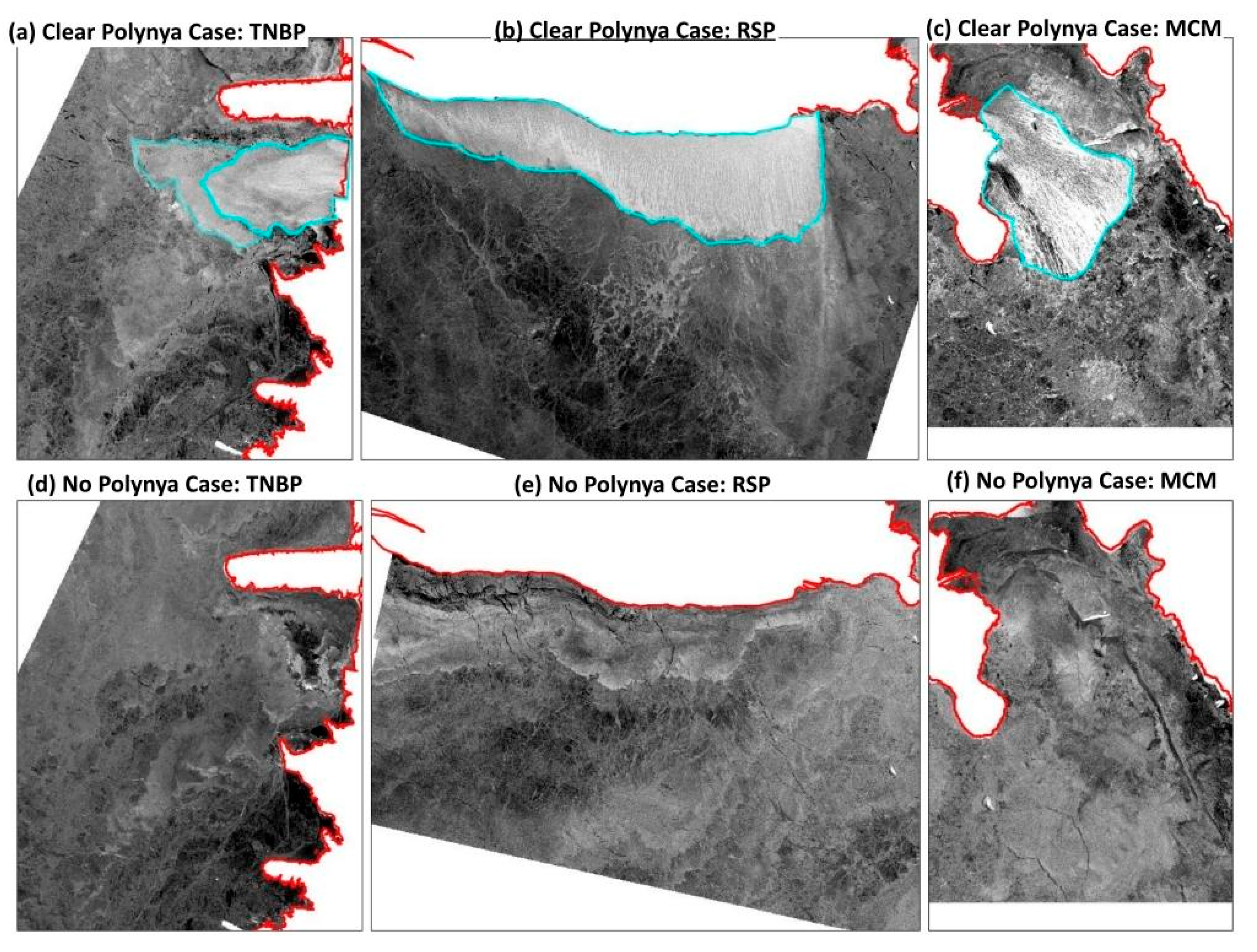
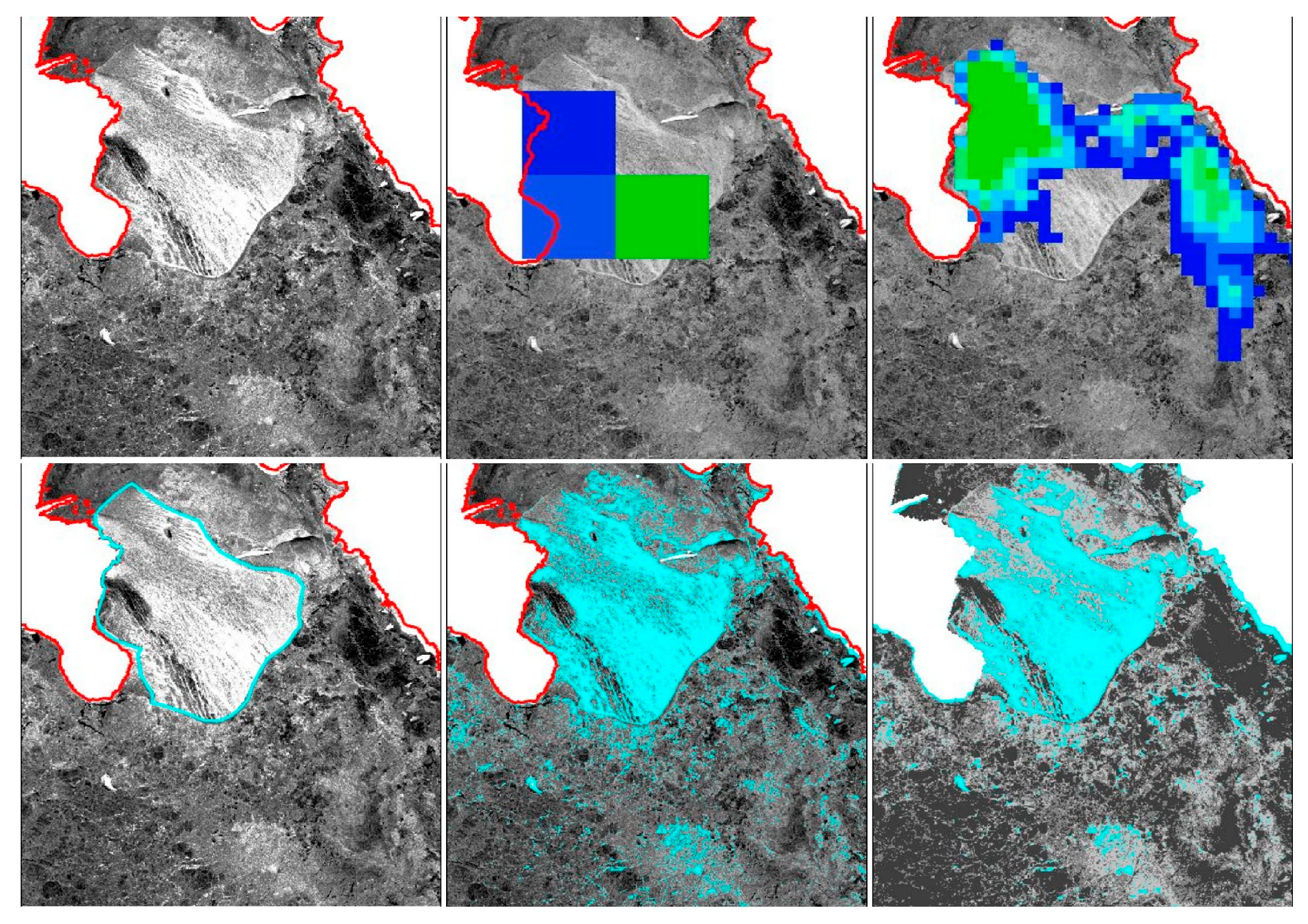
We reviewed the performance of the rule-based and texture-based classifications against manually delineated polynyas that are obtained from S1 imagery. In manual delineation, we identified clear polynyas (Figure 2: Top row) as ones with clearly visually identifiable boundaries. These regions appear bright (high backscatter) on the SAR imagery, as they often occur during or after strong wind events. We also identified S1 scenes that confidently contained no polynyas when usual polynya regions would have transitioned into full ice coverage, showing ridges and leads/linear cracks (Figure 2: bottom row).
The validation period covers winter and early spring season (April to October) from 2017 to 2020, where S1 scene of each area were acquired every 12 days. The RSP had a total of 69 scenes, in which clear polynyas appeared 22 times and no-polynya cases occurred 11 times. For TNBP 51 scenes were examined, clear polynyas were identified in 18, and no-polynya cases in 6. For MCM 70 scenes were examined, clear polynyas were identified in 19, and no-polynya in 36. Polynyas can show complex structures, such as frazil ice and grease ice types which complicate the classification and increase uncertainty when present. Although we examined the characteristics of clear and complex polynyas, we emphasize the clear polynya cases because we are certain about the validated data.

4. Results and Discussions

4.1. Daily PMW Results for the Period 2017–2020

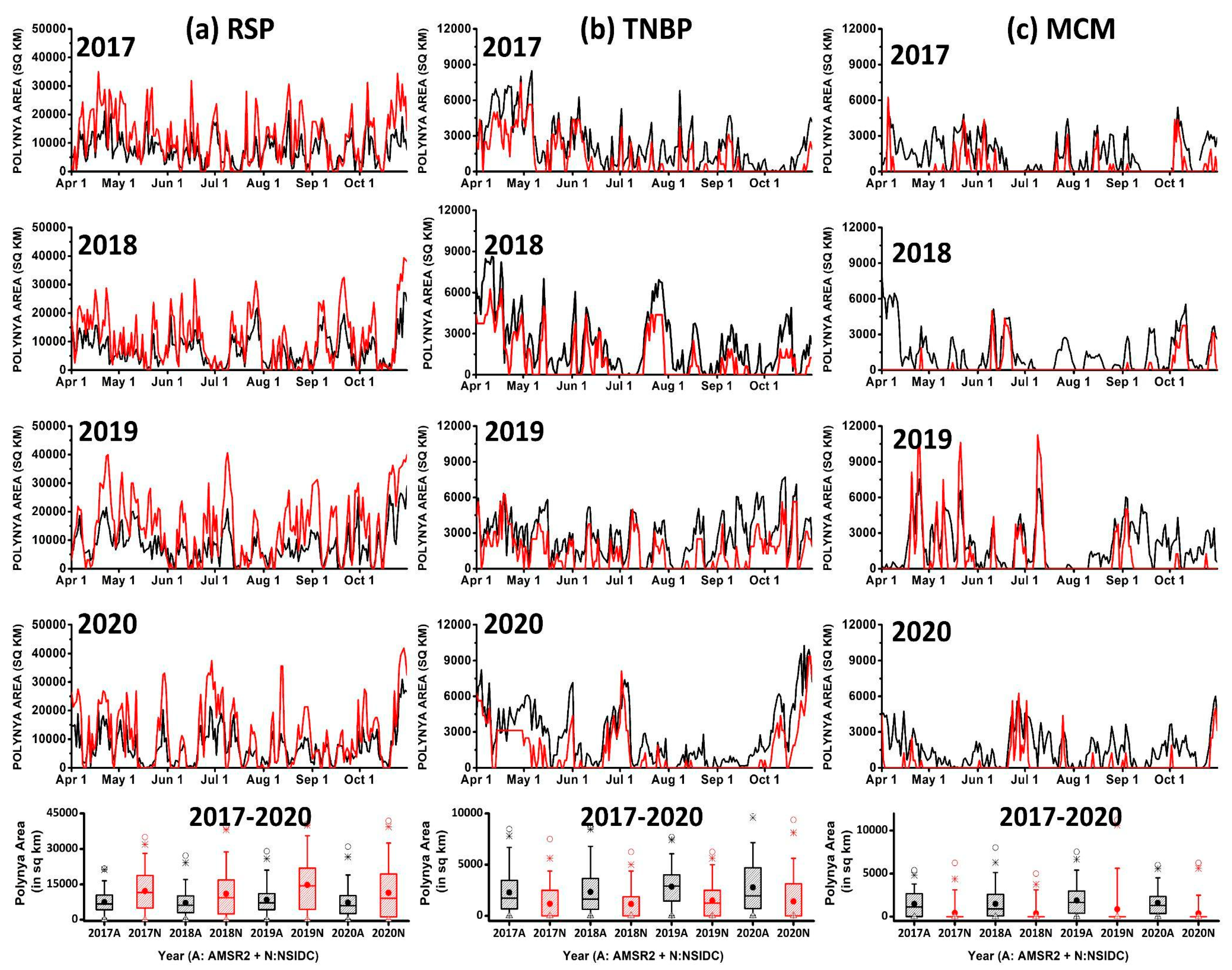
We evaluated data from PMW sensors that are widely used for sea ice studies. We used NSIDC and AMSR2 data to assess the polynya areas for the RSP, TNBP, and MCM regions using the threshold-based method. Using this method, the threshold is set to less than or equal to 60% and all the pixels meeting this criterion are chosen for area calculation. Although the two datasets show good alignment (Figure 3), the largest of the three polynyas (RSP) is overestimated by NSIDC, while the smallest of the three polynyas (MCM) was hardly captured. From the period 2017 to 2020 in MCM, we can observe that PMW datasets reveal high polynya areas for the year 2019 (also reported in recent studies [68]). The range (maximum–minimum) from NSIDC was greater than 10,000 km2 (11,250 km2 refer to Table 1), which is almost double that in the two other years. This example demonstrates that NSIDC generally underestimates the polynyas in MCM, but when these polynyas can be identified, the areas are larger than the ones reported by AMSR2. In the case of TNBP, although the NSIDC and AMSR2 results of the polynya area demonstrated greater correlations over three years in a four-year dataset, the areas did not align spatially on inspection, with NSIDC showing smaller areas compared to AMSR2.
In addition, statistics derived from the daily PMW datasets for the period 2017–2020 from April to October revealed that the NSIDC mean in all the years is nearly double that for AMSR2 in the RSP (Table 2). For TNBP, the mean NSIDC area is lower than that of AMSR2. The difference in percentage between NSIDC and AMSR2 datasets for RSP has NSIDC being 52.8% greater than ASMR2 areas on average. For TNBP, NSIDC has areas that are 64.8% smaller than AMSR2 areas. For the MCM, NSIDC rarely detects polynya in this region, and when identified, it is larger than the AMSR2 values. In summary, NSIDC overestimates larger polynyas and underestimates smaller polynyas compared to AMSR2 (Figure 3). The observed discrepancies could be due to differences in resolution. RSP, being a larger region, the coarser resolution (NSIDC) resulted in overestimation while underestimating the smaller region, TNBP.

4.2. Comparing Large-Scale (PMW) with Fine-Scale (S1) Data

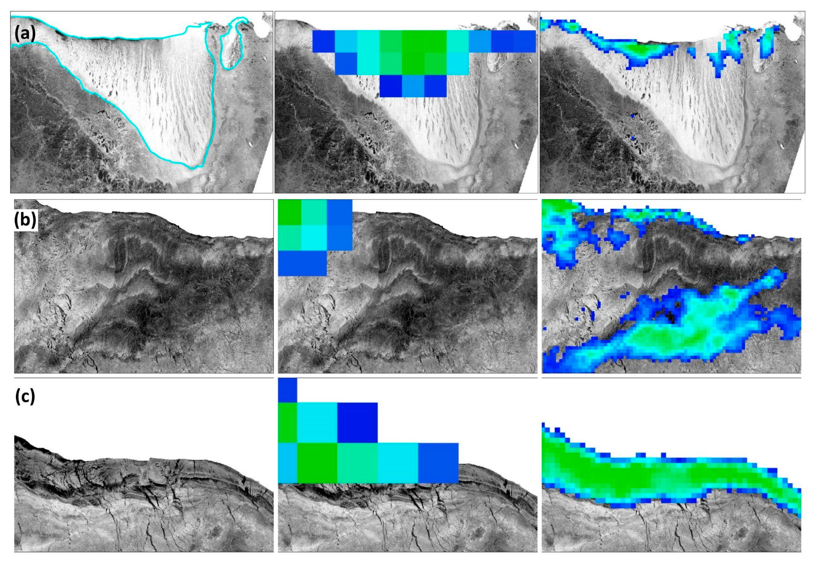
The analysis discussed above shows that both NSIDC and AMSR2 PMW data sets have inconsistencies in detecting polynyas. PMW data solely focuses on concentration values rather than structures; thus, frazil ice/grease ice signatures will be identified within polynya area limits—again overestimating the polynya area as previously reported [26] (Figure 4b: 10 September 2018). On comparing S1 to PMW, S1 data revealed that PMW has less potential in identifying clear polynyas accurately (Figure 4a: 25 July 2020), causing the underestimation of the polynya area in this case. Previous studies [69] reported the efficiency of AMSR2 for thin-ice areas, yet the signals from ice shelves and icebergs can also be misinterpreted in this region (Figure 4b,c: middle row—NSIDC). In addition, AMSR2 is said to be able to identify narrow polynyas, but it is inconsistent in identifying lower-concentration fields (Figure 4b). We often noticed that PMW data could not penetrate liquid water on the top of the ice surface and hence overestimated low sea ice concentrations (Figure 4b) around the onset of melt around September and October months. These regions are easily identified on SAR imagery, as σ0 of such zones is reduced due to desalination (during sea ice formation), making SAR imagery efficient in differentiating open water from early melt onset signals. Additional salient mismatches appeared (Figure 4c) during periods of maximum sea ice extent during September when leads and ridges are often misclassified as polynyas. This is likely due to the presence of open water areas within.
However, S1 data also have a few limitations when it comes to larger polynyas (such as RSP). Firstly, multiple scenes are required to cover the entire stretch beyond S1′s swath. Secondly, the temporal frequency of overpasses is an issue as S1 does not cover the same region on a daily basis.
Our analysis showed that in the case of RSP, NSIDC and AMSR2 misrepresent the structure and size of polynyas relative to our manually delineated regions while also underestimating polynya occurrence, in agreement with previously reported results [26,32]. We noted some discrepancies with RSP, when 11 out of 69 scenes turned out to be days without polynya, while 7 of those days were reported as polynya days by NSIDC and 10 by AMSR2. At MCM, several clear polynyas smaller than the NSIDC pixel size are not detected by NSIDC (Figure 5c), thus underestimating their area and presence (Figure 5c). On the other hand, on certain no-polynya days (36 such scenes for MCM according to manual delineation), NSIDC maintained good consistency by only failing 4 times (32 out 36 were in agreement). However, AMSR2, with its higher resolution was able to capture most of the clear polynya events in McMurdo Sound, but failed with no-polynya cases, as it turned out that 25 scenes out of 36 no-polynya scenes were reported as polynyas. In TNB, AMSR2 considers areas with a combination of broken ice and open water as thin-ice regions (Figure 5a) due to low sea ice concentrations. Therefore, out of six no-polynya cases identified according to manual delineation, five were reported as polynya days by AMSR2. NSIDC, on the other hand, picks up the pixels associated with the Drygalski ice tongue but performed better at identifying no-polynya cases (5 out 6 days matched with our validated data).
Therefore, NSIDC appears to underestimate the polynya area in TNBP, and AMSR2 appears to misinterpret low SIC regions. On the other hand, in MCM, NSIDC barely picks up polynya regions using the 60% threshold.

4.3. Evaluating the S1 Algorithms against the Manually Delineated Data

4.3.1. Texture-Based Unsupervised Classification vs. Rule-Based Supervised Classification

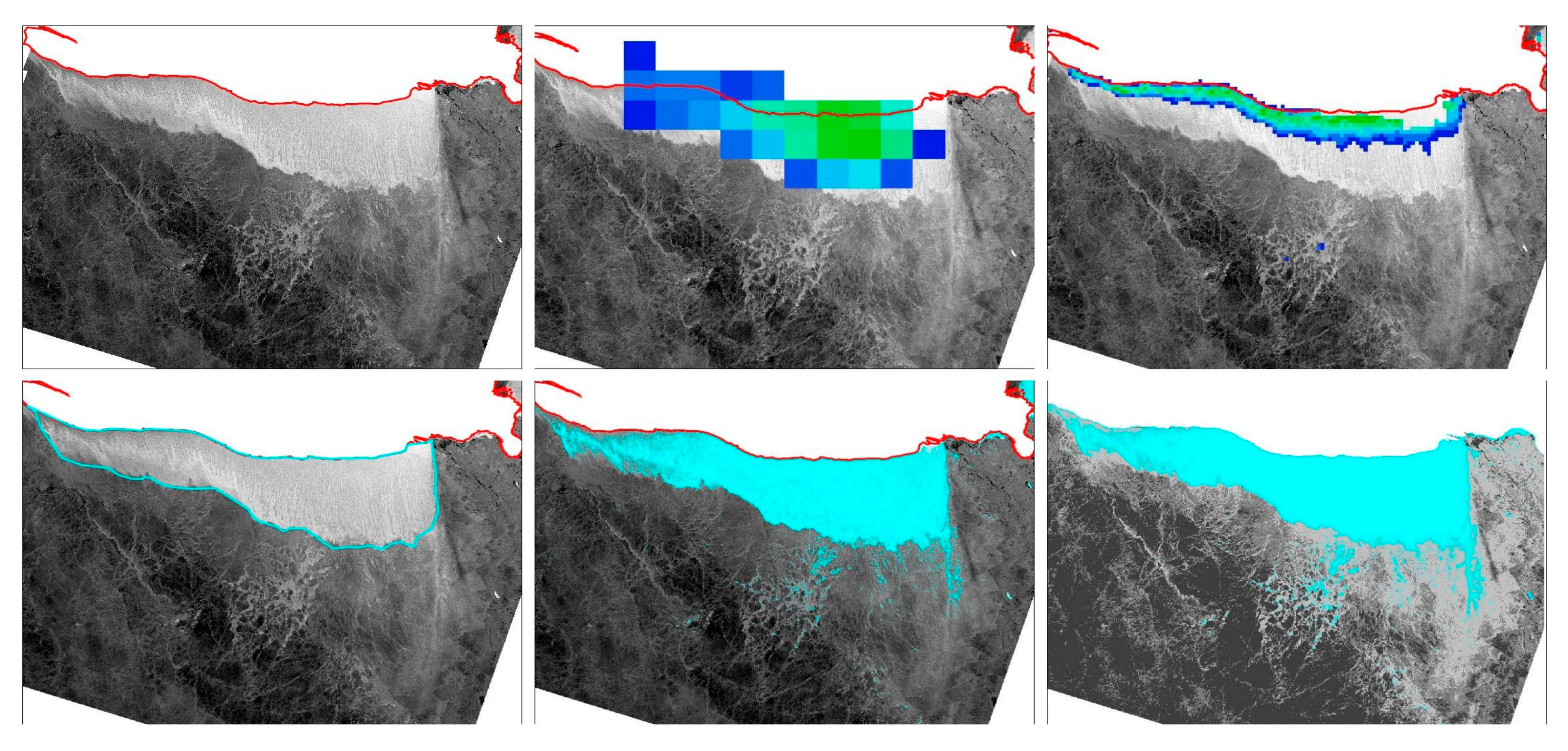
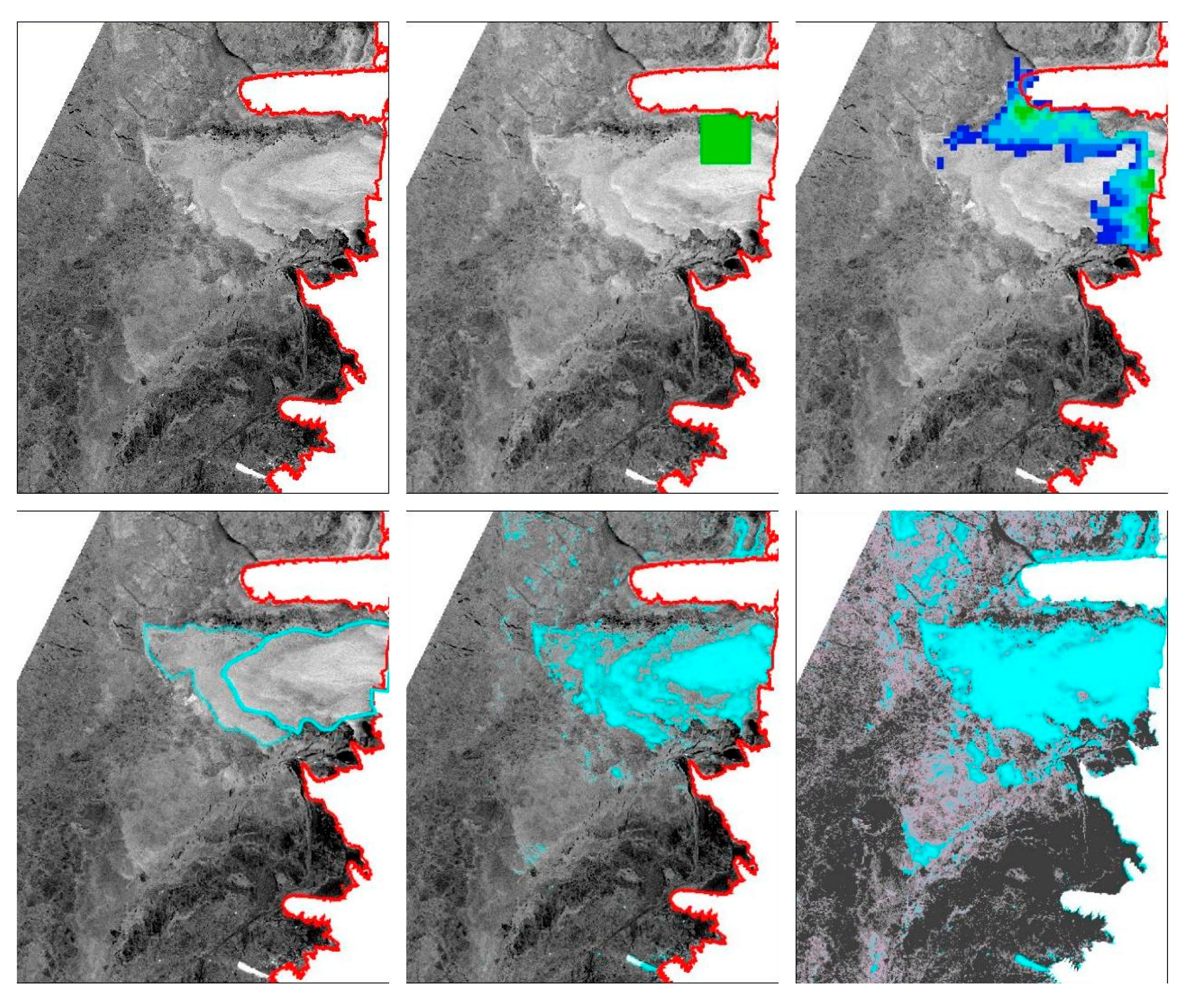
We investigated different types of polynyas using both rule-based and texture-based automatic detection techniques. For RSP, the S1 algorithms are more reliable in identifying the precise periphery of larger polynyas (Figure 6) relative to PMW results. By evaluating the algorithm-generated outcomes against the data generated by manual delineation [38], we can confirm that the rule-based and texture-based techniques are reliable for detecting clear polynya cases in the RSP (refer to Table 3).
For TNBP, it is often reported [70,71,72] that the polynya is maintained by katabatic winds [53], which often force the ice offshore to form multiple boundaries away from the coastline. The polynya begins at the coast of the Drygalski ice tongue and takes the shape of Langmuir circulations [73] in the direction of the winds. When the polynya is in the early stages, often clear boundaries (Figure 7) can be noticed. However, at later stages, we noticed heavily broken ice consisting of small to large floes in the inner parts of the polynya in the SAR imagery. Studies [3,71,72] suggest that such events occur during high wind speeds. Our rule-based algorithm was successful in picking up the thin-ice zones and excluding the broken floes, whereas the texture-based classification included both those regions in a few cases. This is because the texture-based results vary based on the parameters chosen, of which window size is a prominent one. Studies [66] report that the texture information extracted over a large area is preferable. However, in the case of TNBP, as the polynya covers a smaller region, choosing a larger window would lead to poor classification. Hence, a window size of 5 by 5 was set (consistent with all polynyas), which might have misclassified the broken floes between the polynyas. The rule-based approach, being a pixel-based classification, was relatively accurate.
In the case of MCM (Figure 8), the polynyas often need finer spatial resolution to be identified. Occasionally, the clear polynyas are <1000 km2 (Figure 4c) in this region. We noticed that the polynya zone in this region is often impacted by fast ice and active glacier tongues. However, clear polynyas stand out from fast ice areas in the S1 data due to decreased backscatter resulting from low saline (for multiyear ice) fast-ice regions. As a side note, AMSR2 sensors are also capable of identifying thin-ice zones relatively well but often include fast-ice regions. In our analysis, the rule-based results showed better agreement with S1 manually delineated data because the rule-based results identified polynya areas based on only backscatter values for particular pixels. The texture-based results instead operate on the window size chosen, so smaller polynyas, such as TNBP and MCM, were often misclassified.

4.3.2. Clear Polynya Cases

This section describes the statistics for how different techniques perform where clear polynya can be manually delineated. Polynya areas derived from PMW and through S1-based automated techniques are assessed in the following for each polynya. Our S1 rule-based and texture-based schemes demonstrated the potential of S1 in identifying clear polynya zones automatically, as well as the need for finer resolution for polynya studies.
For RSP, our analysis (see Figure 9 right column) shows that NSIDC data often overestimates the clear polynyas relative to manually delineated areas, and AMSR2 underestimates relative to manually delineated S1 areas (Table 3). The means of rule-based (Table 3) polynya areas are well correlated with the means of manually digitized areas, while texture-based results slightly underestimate for the RSP case. The rule-based classification is solely based on co-polarized (HH) backscatter intensity that captures the pixels as supervised by the rule and focuses on the intensity that is within the range set. However, there were instances during non-clear polynya cases (reported later) when even rule-based algorithms were unsuccessful because intensities were close to thresholds used in the classification. We also noticed that a few cases of clear polynyas were associated with extremely bright reflectance of −4 dB and over. This could possibly be due to sources of frost flower aerosol at the Ross Ice Shelf that are reported in some studies [74]. These frost flowers are patches of saline ice crystals [64] that generally grow on newly forming ice and may drastically increase the roughness of the surface. As the results from texture rely on the window size compared to the rule-based, which is a pixel-wise approach, errors are enhanced in texture-based results compared to rule-based. This might be one possibility for justifying the behavior of texture-based results that generally failed compared to rule-based.
Therefore, for RSP, although texture-based results were better than PMW data, rule-based supervised algorithm areas are better correlated with manually delineated areas (Table 3).
In the case of TNBP, the algorithm-based polynya areas were slightly greater than the manually delineated values. From both the PMW results, although AMSR2 values seem to match statistically (Table 3, Mean of AMSR2: around 3270 km2 and S1-Manual Delineation: around 3550 km2), the areas identified were spatially different. This is because often AMSR2 datasets retrieved deformed zones (broken ice floes) that are common in TNBP. For manual delineation in the case of TNBP, the first clear boundary is considered, rather than the broken floes in the further areas beyond the clear boundary. For clear polynya cases, the gaps between polynyas are smaller, hence the results are comparable. In TNBP, both S1-based algorithms performed similarly and the interquartile range (IR) of texture, manual, and AMSR2 matched well.
For smaller polynyas, such as MCM, the low resolution of the NSIDC data could hardly pick up clear polynyas (Figure 7) or over-estimated areas when polynyas were detected. AMSR2, on the other hand, compares better with S1 manually delineated areas when there are clear polynyas, whereas several smaller size polynyas are often overestimated by AMSR2 (see the mean of MCM from Table 3). AMSR2 is also unable to separate mixed signals from broken ice/floes as well as fast-ice zones (previously reported [68]) in MCM. However, AMSR2 results were better than our S1 texture-based algorithm for MCM. Rule-based (about 2060 km2 mean) results are in good accord with manually delineated areas (around 2000 km2).
Our results from clear polynya studies report that NSIDC was unable to identify polynya at times when there is a clear polynya (Table 3, minimum values). AMSR2 identified the presence of polynya in clear cases, underestimated the area in RSP and TNBP, and overestimated most of the time in MCM.

4.3.3. All Scenes (Period: 2017–2020)

To be comprehensive, we also evaluated the performance of different techniques (PMW-based and S1-based against manually delineated values) for the combined period of 2017–2020, for all scenes. This includes cases where a manually delineated area is highly uncertain. This category includes the non-clear polynyas and also periods where no polynya could be observed. Previous studies suggest that the RSP is Antarctica’s largest recurring polynya [75], with an average area of 27,000 km2 [76] (our clear polynyas report a mean of 21,500 km2 for manually delineated areas). Studies [14] also suggest the RSP can expand to as large as 50,000 km2 depending on environmental conditions, whereas our statistics from the manually delineated areas reported a maximum of around 42,000 km2 from our samples. Comparing interquartile ranges from PMW data with S1 shows that the RSP is often over-estimated with NSIDC datasets (Interquartile region (IR): 18,125 km2) and underestimated with AMSR2 (IR: 7021 km2) against the manually delineated S1 values (IR: 13,615 km2). S1-based algorithms, on the other hand, show good agreement with manually derived data (Table 4). The IR of texture-based data was around 12,000 km2, and rule-based was around 13,000 km2, which is in close agreement with manually outlined areas (see Table 4). For the entire period 2017–2020, considering all types together, our results demonstrate that there is close agreement between the mean values of rule-based (13,131 km2) algorithms and manually derived (13,615 km2) results. NSIDC, on the other hand, showed an average of about 14,000 km2 and 8100 km2 for AMSR2, suggesting cases of overestimation and underestimation, respectively, (refer to Figure 9) against S1 manually delineated values.
For TNBP, the mean values for the combined period of 2017–2020 (see Table 4) showed that NSIDC (around 1100 km2) often under-represented the polynya area, while AMSR2 (2360 km2) matched well with the manually delineated values (2312 km2). S1-based algorithms, on the other hand, showed somewhat greater values. Previous studies [70] suggested that the TNBP varies between 1300 km2 and 5000 km2 on average. Alternatively, our results from manually delineated clear polynyas report a maximum of about 7500 km2 which is greater than the upper bound of the previously [70] reported results. S1 algorithms appear to perform well in this region relative to the manual delineation reference value, as they can separate the broken floes within polynya in this region. Our results report that, on average, winter polynyas generally fluctuated between 700 km2 (minimum value) and a maximum of 7500 km2, the maximum value agreeing with previous studies reporting that the TNBP fluctuates around 4000–8000 km2 in their growing phases [3,70] (refer Figure 9).
For MCM, NSIDC could barely detect any polynyas because of the low resolution (Table 4). However, there are cases when polynyas occur over larger spatial scales that are detected by NSIDC, but the areas are often overestimated in such instances. One such case was found in May 2019, where the NSIDC data were almost double (10,625 km2) the manually delineated value (5426 km2) for that particular day. This suggests that NSIDC data often underestimates the clear (small-scale) polynyas at MCM and overestimates when identified. AMSR2 instead picks up lower concentration regions in this region yet disregards the fast-ice [68] information that is critical in this region, resulting in an overestimation of values (mean of 1484 km2) against S1 manually delineated ones (mean around 710 km2). S1-based algorithm area values, particularly texture-based, are closer to the manually delineated ones (710 km2) in this region (Table 4 and Figure 9). The interquartile range data, on the other hand, reports that areas from both the S1-based algorithms (1392 km2 for rule-based and 1005 km2 for texture-based) are in accord with manually delineated ones (1330 km2), while NSIDC is quite low (less than 1000 km2) and AMSR2 is higher (around 2400 km2).
To conclude, our results demonstrate that both the PMW-based areas derived from NSIDC and AMSR2 are strongly related to each other (Table 1). When compared to S1-based manually delineated S1 values, correlations are significantly weaker (p < 0.05) for all three polynyas (Table 5). On comparing the S1 algorithms (rule-based and texture-based) with the manually delineated S1 values for all three polynyas, we noticed significant correlations greater than 0.7 for texture-based and greater than 0.8 for rule-based results (Table 5). On a final note, the rule-based algorithm was the best among all the techniques and is in better agreement with S1 manually delineated values. The correlations with texture-based areas against the manually delineated one (refer to Table 5) while the rule-based algorithms showed the best match of all the techniques. The correlations of S1 (rule- and texture-based) against manually delineated values were greater for all three polynyas (refer to Table 5).
Our results therefore imply that the rule-based areas generated from the S1 supervised approach are in better agreement with manually delineated areas. Therefore, our analysis shows that between rule-based and texture-based algorithms that are based on S1 data, rule-based supervised classification is often close to manually delineated areas and is efficient in identifying clear polynyas accurately. Texture-based results, on the other hand, displayed more errors for smaller polynyas, such as TNBP and MCM, probably due to window size during texture analysis.

5. Conclusions

We have completed a comprehensive review and analysis of polynya properties within the Ross Sea region from a range of satellite products. Our study highlights the importance of high-resolution information for deriving polynya areas. The results are supported from two automated classification techniques for delineating polynya extents: rule-based, and texture-based using S1 C-band co-polarized data. To evaluate the performance of the techniques, we generated the polynya areas through manual delineation of extent. We demonstrate that these techniques are accurate when we selected clear polynyas for particular environments in the Ross Sea relative to manually delineated polynya areas. Cases of clear polynyas were evaluated against the manually delineated S1 values for both rule-based and texture-based approaches. Cases of non-clear and non-polynya types showed major discrepancies with the PMW data, especially during September and October. Whereas S1 match was still quite satisfactory.
Our automated S1-based results (rule-based and texture-based) achieved better results and worked well for cases of clear polynyas for all three regions (RSP, TNBP, and MCM). In comparison, the S1 algorithms results showed that for RSP, the rule-based approach is more useful than the texture-based approach. TNBP results exhibited better correlations with S1 manually delineated values for rule-based rather than texture-based against S1 delineated regions. We, therefore, conclude that for clear polynyas in RSP, MCM, and TNBP, a simple rule-based approach achieved better results of both (rule-based and texture-based) techniques.
On the other hand, PMW data showed low associations in RSP and TNBP compared to S1 manually delineated areas. MCM showed greater correlations given that the samples that are classified as clear are fewer, and most of the processed data belonged to non-clear polynyas. Additionally, the pixel size of NSIDC (625 km2) is quite coarse compared to S1, and clear polynyas in MCM were quite often smaller than an NSIDC pixel. Therefore, there were very few pixels that matched the area of S1. For RSP, we identified 11 scenes that certainly belonged to zero polynya days according to manual delineation and fewer (less than 10) for TNBP, while 36 were non-polynya cases for MCM. We also found that NSIDC maintained a good agreement with no-polynya cases for TNBP and MCM on PMW datasets, while AMSR2 overestimated most of these days. For RSP, both the PMW reported more than 50% of non-polynya cases as polynya cases.
Moreover, we conclude that high-resolution information on polynyas is likely crucial for understanding the interactions driving these dynamic transitions of polynyas from strong to weak types at such local spatiotemporal scales. One limitation we encountered with S1 data was the discontinuity of images when analyzing SAR data, which is rather essential for understanding small-scale processes. In one of our case studies, we noticed RSP switches from ‘no polynya’ to a ‘clear polynya’ case in only 3 days. This is supported by analysis [5] that states high wind periods bring in anti-cyclonic sea ice motion anomalies throughout the Ross Sea, that are found to persist for 48 h after the wind event. However, as we chose to maintain consistent paths and orbits for the scene selection, choosing to limit the temporal interval gap in the study to a 12-day interval, and we might have overlooked or skipped stronger wind events occasionally that occurred frequently within 12 days. Therefore, we find no ideal satellite product that captures both high spatial and temporal resolution. Furthermore, the transitions from clear (active) polynya to no polynya are quite dynamic and complex, which may require additional information to understand this behavior. The behavior of polynyas can be influenced by the synoptic forcing in the Ross Sea sector that has been previously reported [14,77,78,79,80]. However, our S1 algorithm-generated results in cases with combinations of clear and unclear polynyas displayed (Figure 9 left column) good coordination with manually delineated values, especially for RSP and MCM. This study solely aims at identifying fine-scale polynya information areas using high-resolution SAR C-band S1 automated techniques and does not discuss the driving forces that can influence the transitions of polynyas at finer scales. Deriving such information in the future could aid in a better understanding of polynya mechanisms and their future behavior in a warming environment.

Author Contributions

Conceptualization and methodology: A.M., J.R. and G.K.B.; data preparation: B.J. and G.K.B.; data processing and writing—original draft preparation: G.K.B., A.M. and J.R.; supervision, validation, and formal analysis: J.R. and A.M.; funding acquisition and project administration: J.R. and A.M. All authors contributed to final editing. All authors have read and agreed to the published version of the manuscript.

Funding

This research is funded by the New Zealand Antarctic Science Platform (Grant Number ANTA1801) (https://www.antarcticscienceplatform.org.nz/ (accessed on 8 May 2023)).

Data Availability Statement

Not applicable.

Acknowledgments

We thank the National Snow and Ice Data Center for the provision of the 25 km NSIDC sea ice concentration data (https://nsidc.org/ (accessed on 8 May 2023)). Additionally, the University of Bremen, Institute of Environmental Physics for the provision of AMSR2 data (https://seaice.uni-bremen.de/ (accessed on 8 May 2023)), and the European Space Agency (ESA) for the provision of Sentinel-1 high-resolution sea ice data and analysis software (SNAP).

Conflicts of Interest

The authors declare no conflict of interest.

Appendix A. GLCM Parameters Computations Used in the Paper

If G is the number of gray levels, then,
Contrast measures weights related to the distance from the GLCM diagonal. Generally, when i and j are equal, the cell is on the diagonal and (ij) = 0. These values represent pixels entirely similar to their neighbor, so they are given a weight of 0 (no contrast). If i and j differ by 1, there is a small contrast, and the weight is 1. If i and j differ by 2, contrast is increasing, and the weight is 4. So, the weights continue to increase as the square of (ij).
i , j = 0 G 1 P i j ( i j ) 2
Entropy, the measure for determining uncertainty, is also used to depict the texture of the image. If all the co-occurrence vector components are the same, the entropy’s magnitude will be a maximum. Entropy is usually classified as a first-degree measure but should properly be a “zeroth” degree. Pij is always between 0 and 1, because it is a probability. Therefore, log(Pij) will always be 0 or negative. The smaller the value of Pij (i.e., the less common the occurrence of that pixel combination), the larger the absolute value of log (Pij), and the (−1) multiplier in the entropy equation makes each term positive. Therefore, the smaller the Pij value, the greater the weight, and the greater the value of −[Pij × log(Pij)].
i , j = 0 G 1 P i , j ( l o g P i , j )
Dissimilarity: Instead of weights increasing as squares as one moves away from the diagonal as Contrast did, the dissimilarity weights increase linearly
i , j = 0 G 1 P i j | i j |
Angular Second Moment (ASM): ASM uses each Pij as a weight for itself. High values of ASM occur when the window is very orderly.
i , j = 0 G 1 { ( P i , j ) } 2
Mean: The Mean in GLCM is a weight of a pixel value not by its frequency of occurrence by itself but by its frequency of its occurrence in combination with a certain neighbor pixel value. So, GLCM means is not simply the average of all the original pixel values in the image window.
i , j = 0 G 1 i P i , j
Correlation: This measures the linear dependency of grey levels on those of neighboring pixels. Correlation between pixels means that there is a predictable and linear relationship between the two neighboring pixels within the window, expressed by the regression equation. A high correlation texture means high predictability of pixel relationships. Single patches of a particular class usually have a higher correlation value within them than between adjacent objects.
i , j = 0 G 1 i µ i j µ j P i , j σ i 2 σ j 2

References

  1. Morales Maqueda, M.A.; Willmott, A.J.; Biggs, N.R.T. Polynya Dynamics: A Review of Observations and Modeling: Polynya dynamics-observations and modeling. Rev. Geophys. 2004, 42, 116. [Google Scholar] [CrossRef]
  2. Martin, S. Polynyas. In Encyclopedia of Ocean Sciences; Elsevier: Amsterdam, The Netherlands, 2001; pp. 2241–2247. ISBN 978-0-12-227430-5. [Google Scholar]
  3. Hollands, T.; Dierking, W. Dynamics of the Terra Nova Bay Polynya: The Potential of Multi-Sensor Satellite Observations. Remote Sens. Environ. 2016, 187, 30–48. [Google Scholar] [CrossRef]
  4. Jiang, L.; Ma, Y.; Chen, F.; Liu, J.; Yao, W.; Qiu, Y.; Zhang, S. Trends in the Stability of Antarctic Coastal Polynyas and the Role of Topographic Forcing Factors. Remote Sens. 2020, 12, 1043. [Google Scholar] [CrossRef]
  5. Dale, E.R.; McDonald, A.J.; Coggins, J.H.J.; Rack, W. Atmospheric Forcing of Sea Ice Anomalies in the Ross Sea Polynya Region. Cryosphere Discuss. 2016, 11, 267–280. [Google Scholar] [CrossRef]
  6. Tamura, T.; Ohshima, K.I.; Fraser, A.D.; Williams, G.D. Sea Ice Production Variability in Antarctic Coastal Polynyas. J. Geophys. Res. Oceans 2016, 121, 2967–2979. [Google Scholar] [CrossRef]
  7. Adams, S. Monitoring of Thin Sea Ice within Polynyas Using MODIS Data Beobachtung Des Dünnen Meereises in Polynjen Anhand von MODIS Daten. Ph.D. Thesis, University of Trier, Trier, Germany, 18 December 2012. [Google Scholar]
  8. Massom, R.A.; Harris, P.T.; Michael, K.J.; Potter, M.J. The Distribution and Formative Processes of Latent-Heat Polynyas in East Antarctica. Ann. Glaciol. 1998, 27, 420–426. [Google Scholar] [CrossRef]
  9. Barber, D.G.; Massom, R.A. Chapter 1 The Role of Sea Ice in Arctic and Antarctic Polynyas. In Elsevier Oceanography Series; Elsevier: Amsterdam, The Netherlands, 2007; Volume 74, pp. 1–54. ISBN 978-0-444-52952-7. [Google Scholar]
  10. Sea Ice Features: Polynyas | National Snow and Ice Data Center. Available online: https://nsidc.org/cryosphere/seaice/characteristics/polynyas.html (accessed on 30 May 2022).
  11. Gordon, A.L.; Comiso, J.C. Polynyas in the Southern Ocean. Sci. Am. 1988, 258, 90–97. [Google Scholar] [CrossRef]
  12. Kashiwase, H.; Ohshima, K.I.; Nakata, K.; Tamura, T. Improved SSM/I Thin Ice Algorithm with Ice Type Discrimination in Coastal Polynyas. J. Atmos. Ocean. Technol. 2021, 38, 823–835. [Google Scholar] [CrossRef]
  13. Castagno, P.; Capozzi, V.; DiTullio, G.R.; Falco, P.; Fusco, G.; Rintoul, S.R.; Spezie, G.; Budillon, G. Rebound of Shelf Water Salinity in the Ross Sea. Nat. Commun. 2019, 10, 5441. [Google Scholar] [CrossRef]
  14. Park, J.; Kim, H.-C.; Jo, Y.-H.; Kidwell, A.; Hwang, J. Multi-Temporal Variation of the Ross Sea Polynya in Response to Climate Forcings. Polar Res. 2018, 37, 1444891. [Google Scholar] [CrossRef]
  15. Carrasco, J.F.; Bromwich, D.H. Mesoscale Cyclogenesis Dynamics over the Southwestern Ross Sea, Antarctica. J. Geophys. Res. 1993, 98, 12973. [Google Scholar] [CrossRef]
  16. Hoppema, M.; Anderson, L.G. Chapter 6 Biogeochemistry of Polynyas and Their Role in Sequestration of Anthropogenic Constituents. In Elsevier Oceanography Series; Elsevier: Amsterdam, The Netherlands, 2007; Volume 74, pp. 193–221. ISBN 978-0-444-52952-7. [Google Scholar]
  17. Arrigo, K.R. Phytoplankton Dynamics within 37 Antarctic Coastal Polynya Systems. J. Geophys. Res. 2003, 108, 3271. [Google Scholar] [CrossRef]
  18. Wang, X.; Zhang, Z.; Wang, X.; Vihma, T.; Zhou, M.; Yu, L.; Uotila, P.; Sein, D.V. Impacts of Strong Wind Events on Sea Ice and Water Mass Properties in Antarctic Coastal Polynyas. Clim. Dyn. 2021, 57, 3505–3528. [Google Scholar] [CrossRef]
  19. Christie, F.D.W.; Benham, T.J.; Batchelor, C.L.; Rack, W.; Montelli, A.; Dowdeswell, J.A. Antarctic ice-shelf advance driven by anomalous atmospheric and sea-ice circulation. Nat. Geosci. 2022, 15, 356–362. [Google Scholar] [CrossRef]
  20. Rack, W.; Price, D.; Haas, C.; Langhorne, P.J.; Leonard, G.H. Sea Ice Thickness in the Western Ross Sea. Geophys. Res. Lett. 2021, 48, e2020GL090866. [Google Scholar] [CrossRef]
  21. Ohshima, K.I.; Nihashi, S.; Iwamoto, K. Global View of Sea-Ice Production in Polynyas and Its Linkage to Dense/Bottom Water Formation. Geosci. Lett. 2016, 3, 13. [Google Scholar] [CrossRef]
  22. Mathiot, P.; Jourdain, N.C.; Barnier, B.; Gallée, H.; Molines, J.M.; Le Sommer, J.; Penduff, T. Sensitivity of Coastal Polynyas and High-Salinity Shelf Water Production in the Ross Sea, Antarctica, to the Atmospheric Forcing. Ocean. Dyn. 2012, 62, 701–723. [Google Scholar] [CrossRef]
  23. Mezgec, K.; Stenni, B.; Crosta, X.; Masson-Delmotte, V.; Baroni, C.; Braida, M.; Ciardini, V.; Colizza, E.; Melis, R.; Salvatore, M.C.; et al. Holocene Sea Ice Variability Driven by Wind and Polynya Efficiency in the Ross Sea. Nat. Commun. 2017, 8, 1334. [Google Scholar] [CrossRef]
  24. Kern, S.; Spreen, G.; Kaleschke, L.; de La Rosa, S.; Heygster, G. Polynya Signature Simulation Method Polynya Area in Comparison to AMSR-E 89 GHz Sea-Ice Concentrations in the Ross Sea and off the Adélie Coast, Antarctica, for 2002–05: First Results. Ann. Glaciol. 2007, 46, 409–418. [Google Scholar] [CrossRef]
  25. Markus, T.; Burns, B.A. Detection of Coastal Polynyas with Passive Microwave Data. Ann. Glaciol. 1993, 17, 351–355. [Google Scholar] [CrossRef]
  26. Kwok, R. Sea Ice Concentration Estimates from Satellite Passive Microwave Radiometry and Openings from SAR Ice Motion: Sea Ice Concentration and Sar Openings. Geophys. Res. Lett. 2002, 29, 25-1–25-4. [Google Scholar] [CrossRef]
  27. Martin, S. Estimation of the Thin Ice Thickness and Heat Flux for the Chukchi Sea Alaskan Coast Polynya from Special Sensor Microwave/Imager Data, 1990–2001. J. Geophys. Res. 2004, 109, C10012. [Google Scholar] [CrossRef]
  28. Adams, S.; Willmes, S.; Heinemann, G.; Rozman, P.; Timmermann, R.; Schröder, D. Evaluation of Simulated Sea-Ice Concentrations from Sea-Ice/Ocean Models Using Satellite Data and Polynya Classification Methods. Polar Res. 2011, 30, 7124. [Google Scholar] [CrossRef]
  29. Cheng, Z.; Pang, X.; Zhao, X.; Stein, A. Heat Flux Sources Analysis to the Ross Ice Shelf Polynya Ice Production Time Series and the Impact of Wind Forcing. Remote Sens. 2019, 11, 188. [Google Scholar] [CrossRef]
  30. Melsheimer, C. ASI Version 5 Sea Ice Concentration User Guide; University of Bremen: Bremen, Germany, 2019; Volume 10. [Google Scholar]
  31. Ivanova, N.; Pedersen, L.T.; Tonboe, R.T.; Kern, S.; Heygster, G.; Lavergne, T.; Sørensen, A.; Saldo, R.; Dybkjær, G.; Brucker, L.; et al. Inter-Comparison and Evaluation of Sea Ice Algorithms: Towards Further Identification of Challenges and Optimal Approach Using Passive Microwave Observations. Cryosphere 2015, 9, 1797–1817. [Google Scholar] [CrossRef]
  32. Martin, S.; Drucker, R.S.; Kwok, R. The Areas and Ice Production of the Western and Central Ross Sea Polynyas, 1992–2002, and Their Relation to the B-15 and C-19 Iceberg Events of 2000 and 2002. J. Mar. Syst. 2007, 68, 201–214. [Google Scholar] [CrossRef]
  33. Holland, P.R.; Kwok, R. Wind-Driven Trends in Antarctic Sea-Ice Drift. Nat. Geosci. 2012, 5, 872–875. [Google Scholar] [CrossRef]
  34. Mohrmann, M.; Heuzé, C.; Swart, S. Southern Ocean Polynyas in CMIP6 Models. Cryosphere 2021, 15, 4281–4313. [Google Scholar] [CrossRef]
  35. Farooq, U.; Rack, W.; McDonald, A.; Howell, S. Long-Term Analysis of Sea Ice Drift in the Western Ross Sea, Antarctica, at High and Low Spatial Resolution. Remote Sens. 2020, 12, 1402. [Google Scholar] [CrossRef]
  36. Jolly, B.; Kuma, P.; McDonald, A.; Parsons, S. An Analysis of the Cloud Environment over the Ross Sea and Ross Ice Shelf Using CloudSat/CALIPSO Satellite Observations: The Importance of Synoptic Forcing. Atmos. Chem. Phys. 2018, 18, 9723–9739. [Google Scholar] [CrossRef]
  37. Willmes, S.; Krumpen, T.; Adams, S.; Rabenstein, L.; Haas, C.; Hoelemann, J.; Heinemann, G. Cross-Validation of Polynya Monitoring Methods from Multisensor Satellite and Airborne Data: A Case. Can. J. Remote Sens. 2010, 36, S13–S25. [Google Scholar] [CrossRef]
  38. Dai, L.; Xie, H.; Ackley, S.F.; Mestas-Nuñez, A.M. Ice Production in Ross Ice Shelf Polynyas during 2017–2018 from Sentinel–1 SAR Images. Remote Sens. 2020, 12, 1484. [Google Scholar] [CrossRef]
  39. Chen, S.; Shokr, M.; Li, X.; Ye, Y.; Zhang, Z.; Hui, F.; Cheng, X. MYI Floes Identification Based on the Texture and Shape Feature from Dual-Polarized Sentinel-1 Imagery. Remote Sens. 2020, 12, 3221. [Google Scholar] [CrossRef]
  40. Aldenhoff, W.; Eriksson, L.E.B.; Ye, Y.; Heuze, C. First-Year and Multiyear Sea Ice Incidence Angle Normalization of Dual-Polarized Sentinel-1 SAR Images in the Beaufort Sea. IEEE J. Sel. Top. Appl. Earth Obs. Remote Sens. 2020, 13, 1540–1550. [Google Scholar] [CrossRef]
  41. Aldenhoff, W.; Heuzé, C.; Eriksson, L.E.B. Comparison of Ice/Water Classification in Fram Strait from C- and L-Band SAR Imagery. Ann. Glaciol. 2018, 59, 112–123. [Google Scholar] [CrossRef]
  42. Lohse, J.; Doulgeris, A.P.; Dierking, W. Mapping Sea-Ice Types from Sentinel-1 Considering the Surface-Type Dependent Effect of Incidence Angle. Ann. Glaciol. 2020, 61, 260–270. [Google Scholar] [CrossRef]
  43. Lohse, J.; Doulgeris, A.P.; Dierking, W. Incident Angle Dependence of Sentinel-1 Texture Features for Sea Ice Classification. Remote Sens. 2021, 13, 552. [Google Scholar] [CrossRef]
  44. Park, J.-W.; Korosov, A.A.; Babiker, M.; Won, J.-S.; Hansen, M.W.; Kim, H.-C. Classification of sea ice types in Sentinel-1 synthetic aperture radar images. Cryosphere 2020, 14, 2629–2645. [Google Scholar] [CrossRef]
  45. Murashkin, D.; Spreen, G.; Huntemann, M.; Dierking, W. Method for Detection of Leads from Sentinel-1 SAR Images. Ann. Glaciol. 2018, 59, 124–136. [Google Scholar] [CrossRef]
  46. Aldenhoff, W.; Berg, A.; Eriksson, L.E.B. Sea Ice Concentration Estimation from Sentinel-1 Synthetic Aperture Radar Images over the Fram Strait. In Proceedings of the 2016 IEEE International Geoscience and Remote Sensing Symposium (IGARSS), Beijing, China, 10–15 July 2016; pp. 7675–7677. [Google Scholar]
  47. Boulze, H.; Korosov, A.; Brajard, J. Classification of Sea Ice Types in Sentinel-1 SAR Data Using Convolutional Neural Networks. Remote Sens. 2020, 12, 2165. [Google Scholar] [CrossRef]
  48. Scharien, R.; Segal, R.; Yackel, J.; Howell, S.; Nasonova, S. Linking Winter and Spring Thermodynamic Sea-Ice States at Critical Scales Using an Object-Based Image Analysis of Sentinel-1. Ann. Glaciol. 2018, 59, 148–162. [Google Scholar] [CrossRef]
  49. Drucker, R.; Martin, S.; Kwok, R. Sea Ice Production and Export from Coastal Polynyas in the Weddell and Ross Seas: Weddell and Ross Sea Ice Production. Geophys. Res. Lett. 2011, 38, 17. [Google Scholar] [CrossRef]
  50. Lei, R.; Gui, D.; Yuan, Z.; Pang, X.; Tao, D.; Zhai, M. Characterization of the Unprecedented Polynya Events North of Greenland in 2017/2018 Using Remote Sensing and Reanalysis Data. Acta Oceanol. Sin. 2020, 39, 5–17. [Google Scholar] [CrossRef]
  51. Soh, L.-K.; Tsatsoulis, C. Texture Analysis of SAR Sea Ice Imagery Using Gray Level Co-Occurrence Matrices. IEEE Trans. Geosci. Remote Sens. 1999, 37, 780–795. [Google Scholar] [CrossRef]
  52. Hong, D.-B.; Yang, C.-S. Automatic Discrimination Approach of Sea Ice in the Arctic Ocean Using Sentinel-1 Extra Wide Swath Dual-Polarized SAR Data. Int. J. Remote Sens. 2018, 39, 4469–4483. [Google Scholar] [CrossRef]
  53. Petrelli, P.; Bindoff, N.L.; Bergamasco, A. The Sea Ice Dynamics of Terra Nova Bay and Ross Ice Shelf Polynyas during a Spring and Winter Simulation. J. Geophys. Res. 2008, 113, C09003. [Google Scholar] [CrossRef]
  54. Price, D. Assessment of Antarctic Sea Ice by Surface Validated Satellite Measurements. Ph.D. Thesis, University of Canterbury, Christchurch, New Zealand, 2014. [Google Scholar] [CrossRef]
  55. Meier, W.; Fetterer, F.; Windnagel, A.; Stewart, S. NOAA/NSIDC Climate Data Record of Passive Microwave Sea Ice Concentration; Version 4; National Snow and Ice Data Center: Boulder, CO, USA, 2021. [Google Scholar]
  56. Vichi, M. A Statistical Definition of the Antarctic Marginal Ice Zone. Cryosphere 2021, 16, 4087–4106. [Google Scholar] [CrossRef]
  57. Sentinel-1 SAR—Technical Guide—Sentinel Online—Sentinel Online. Available online: https://sentinel.esa.int/web/sentinel/technical-guides/sentinel-1-sar (accessed on 6 July 2022).
  58. SNAP Download—STEP. Available online: https://step.esa.int/main/download/snap-download/ (accessed on 8 May 2023).
  59. Parmiggiani, F. Multi-Year Measurement of Terra Nova Bay Winter Polynya Extents. Eur. Phys. J. Plus 2011, 126, 39. [Google Scholar] [CrossRef]
  60. Yue, B. SAR Sea Ice Recognition Using Texture Methods. Master’s Thesis, University of Waterloo, Waterloo, ON, Canada, 2002. [Google Scholar]
  61. Geldsetzer, T.; Yackel, J.J. Sea Ice Type and Open Water Discrimination Using Dual Co-Polarized C-Band SAR. Can. J. Remote Sens. 2009, 35, 13. [Google Scholar] [CrossRef]
  62. Remote Sensing of Sea Ice in the Northern Sea Route; Springer Praxis Books; Springer: Berlin/Heidelberg, Germany, 2006; ISBN 978-3-540-24448-6.
  63. Classification of Sea Ice Types in ENVISAT Synthetic Aperture Radar Images | IEEE Journals & Magazine | IEEE Xplore. Available online: https://ieeexplore-ieee-org.helicon.vuw.ac.nz/document/6311463 (accessed on 7 July 2022).
  64. Dierking, W. Sea Ice Monitoring by Synthetic Aperture Radar. Oceanography 2013, 26, 100–111. [Google Scholar] [CrossRef]
  65. Shokr, M.E. Evaluation of Second-Order Texture Parameters for Sea Ice Classification from Radar Images. J. Geophys. Res. 1991, 96, 10625. [Google Scholar] [CrossRef]
  66. Gkanatsios, I. Classification of Sea Ice Types for the East Part of Greenland Waters Using SENTINEL 1 Data. Master’s Thesis, The University of Edinburgh, Edinburgh, UK, 2019. [Google Scholar]
  67. McDonald, A.J.; George, S.E.; Woollands, R.M. Can Gravity Waves Significantly Impact PSC Occurrence in the Antarctic? Atmos. Chem. Phys. 2009, 9, 8825–8840. [Google Scholar] [CrossRef]
  68. Leonard, G.H.; Turner, K.E.; Richter, M.E.; Whittaker, M.S.; Smith, I.J. Brief Communication: The Anomalous Winter 2019 Sea-Ice Conditions in McMurdo Sound, Antarctica. Cryosphere 2021, 15, 4999–5006. [Google Scholar] [CrossRef]
  69. Tamura, T.; Ohshima, K.I.; Nihashi, S. Mapping of Sea Ice Production for Antarctic Coastal Polynyas: Mapping of sea ice production. Geophys. Res. Lett. 2008, 35, 2079–2087. [Google Scholar] [CrossRef]
  70. Bromwich, D.H.; Kurtz, D.D. Katabatic Wind Forcing of the Terra Nova Bay Polynya. J. Geophys. Res. 1984, 89, 3561. [Google Scholar] [CrossRef]
  71. Davolio, S.; Buzzi, A. Mechanisms of Antarctic Katabatic Currents near Terra Nova Bay. Tellus A Dyn. Meteorol. Oceanogr. 2002, 54, 187–204. [Google Scholar] [CrossRef]
  72. Breckenridge, C.J.; Radok, U.; Stearns, C.R.; Bromwich, D.H. Katabatic Winds along the Transantarctic Mountains. In Antarctic Research Series; Bromwich, D.H., Stearns, C.R., Eds.; American Geophysical Union: Washington, DC, USA, 1993; Volume 61, pp. 69–92. ISBN 978-0-87590-839-7. [Google Scholar]
  73. Leibovich, S. The Form and Dynamics of Langmuir Circulations. Annu. Rev. Fluid Mech. 1983, 15, 391–427. [Google Scholar] [CrossRef]
  74. Kaleschke, L. Frost Flowers on Sea Ice as a Source of Sea Salt and Their Influence on Tropospheric Halogen Chemistry. Geophys. Res. Lett. 2004, 31, L16114. [Google Scholar] [CrossRef]
  75. Thompson, L.; Smith, M.; Thomson, J.; Stammerjohn, S.; Ackley, S.; Loose, B. Frazil ice growth and production during katabatic wind events in the Ross Sea, Antarctica. Cryosphere 2020, 14, 3329–3347. [Google Scholar] [CrossRef]
  76. Dale, E.R.; Katurji, M.; McDonald, A.J.; Voss, P.; Rack, W.; Seto, D. A Comparison of AMPS Forecasts Near the Ross Sea Polynya With Controlled Meteorological Balloon Observations. J. Geophys. Res. Atmos. 2020, 125, e2019JD030591. [Google Scholar] [CrossRef]
  77. Dale, E.R. Interactions between Changing Weather Patterns and the Antarctic Cryosphere in the Ross Sea Region. Ph.D. Thesis, University of Canterbury, Christchurch, New Zealand, 2020. [Google Scholar] [CrossRef]
  78. Cohen, L.; Dean, S.; Renwick, J. Synoptic Weather Types for the Ross Sea Region, Antarctica. J. Clim. 2013, 26, 636–649. [Google Scholar] [CrossRef]
  79. Coggins, J.H.J.; McDonald, A.J. The Influence of the Amundsen Sea Low on the Winds in the Ross Sea and Surroundings: Insights from a Synoptic Climatology. J. Geophys. Res. Atmos. 2015, 120, 2167–2189. [Google Scholar] [CrossRef]
  80. Renwick, J.A.; Kohout, A.; Dean, S. Atmospheric Forcing of Antarctic Sea Ice on Intraseasonal Time Scales. J. Clim. 2012, 25, 5962–5975. [Google Scholar] [CrossRef]
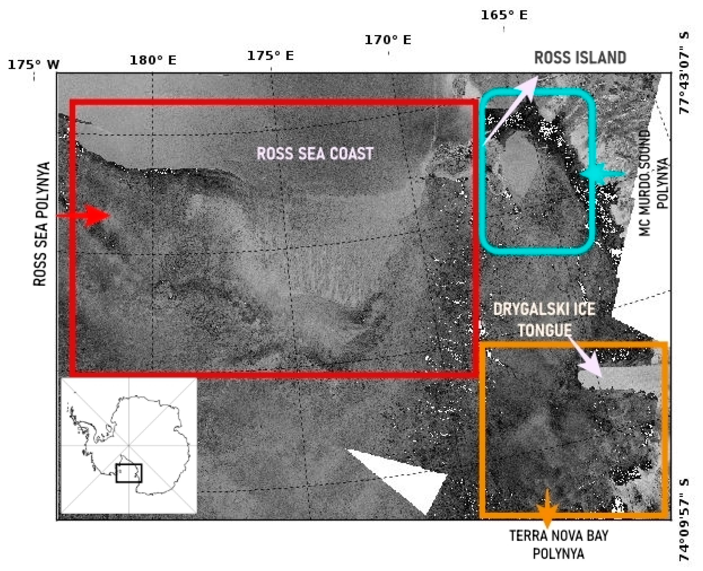
Figure 1. Sentinel-1 data are used to identify the polynya regions considered in the study area. The Sentinel-1 imagery shows the Ross Sea region considered for the study. In Red is the Ross ice shelf Polynya (RSP-Red), Terra Nova Bay Polynya (TNBP) in Orange and Mc Murdo Sound Polynya (MCM) in blue (inset: Antarctica).
Remotesensing 15 02545 g001
Figure 2. All the background figures are of processed Sentinel-1. Red border shows the Ross sector coastline and cyan represents the polynya outline. Clear Polynya (ac) and No Polynya cases (df) for the polynyas TNBP, RSP, and MCM (represented from left to right order). The case (a) for TNBP is deliberately chosen to depict the cases of multiple polynya border polynya, in such cases the first clear boundary is chosen for comparison with the manual delineation. Dates of scenes selected: RSP: 30 August 2020; TNBP: 17 July 2020; and MCM: 2 June 2017.
Remotesensing 15 02545 g002
Figure 3. The top 4 rows represent the Daily Polynya area (in km2) calculated from NSIDC (red) and AMSR2 (black) for the period 2017–2020 for RSP, TNBP, and MCM (left to right). Corresponding boxplots for NSIDC and AMSR2 datasets for the same period are represented in the bottommost row. An interquartile range of 25–75%. The filled circle inside the box represents the mean, the unfilled circle is the maximum value, plus sign represents the minimum value, and an asterisk (*) represents 99% range for the chosen period; (a) RSP; (b) TNBP; (c) MCM.
Remotesensing 15 02545 g003
Figure 4. All the background figures are of processed Sentinel-1. Cases of underestimation and overestimation of RSP (left column represents the manually delineated result) as referenced in cyan (no markings when there are no active polynyas) from S1. Middle column images represent the result from NSIDC, rightmost is the result of AMSR2 with processed S1 in the background. Concentration of green to blue represents low to high concentrations. Dates of scenes displayed (a) 25 July 2020, (b) 10 September 2018, and (c) 18 September 2017.
Remotesensing 15 02545 g004
Figure 5. All the background figures are of processed Sentinel-1. Cases of Underestimation and Overestimation of TNBP and MCM regions (Left to Right order represents the manually delineated reference in cyan (no markings when there are no active polynyas) from S1, NSIDC, AMSR2). Concentration in green–blue represents low to high concentrations. Dates of scenes displayed (a) 12 May 2019, (b) 9 September 2019, (c) 20 July 2017, and (d) 20 August 2018.
Remotesensing 15 02545 g005
Figure 6. All the figures have S1 processed scene as a background and polynya areas obtained through different techniques on the forefront. Top row (left–right) corresponds to a processed S1 scene, polynya area retrieved by NSIDC, and polynya area retrieved by AMSR2 in the foreground. Bottom row (left to right) corresponds to a manually delineated area in cyan, polynya area retrieved by S1′s rule-based approach, and polynya area retrieved by S1′s Texture-based classifications. Dates of S1 scene—30 August 2020.
Remotesensing 15 02545 g006
Figure 7. All the figures have S1 processed scene as a background and polynya areas obtained through different techniques on the forefront. Red border shows the Ross sector coastline and cyan represents the polynya outline. Top row (left–right) corresponds to a processed S1 scene, polynya area retrieved by NSIDC, and polynya area retrieved by AMSR2, respectively, in the foreground. Bottom row (left to right) corresponds to a manually delineated area in cyan, polynya area retrieved by S1′s rule-based approach, and polynya area retrieved by S1′s texture-based classifications. Date of S1 scene used: 17 July 2017.
Remotesensing 15 02545 g007
Figure 8. All the figures have S1 processed scene as a background and polynya areas obtained through different techniques on the forefront. Red border shows the Ross sector coastline and cyan represents the polynya outline. Top row (left–right) corresponds to a processed S1 scene, polynya area retrieved by NSIDC, and polynya area retrieved by AMSR2, respectively, in the foreground. Bottom row (left to right) corresponds to a manually delineated area in cyan, polynya area retrieved by S1′s rule-based approach, and polynya area retrieved by S1′s texture-based classifications. Date of S1 scene used: Clear: 2 June 2017.
Remotesensing 15 02545 g008
Figure 9. Boxplots show a comparison of different techniques. (The left panel) denotes ‘Only Clear Polynyas’ identified by manual delineation using S1, whereas (the right panel) represents ‘All cases together’ (Clear and Non-Clear) for the period 2017–2020 (April–October). An interquartile range of 25–75% defines the box range, while the whisker range is 10–90%. Other statistics include maximum (filled star), minimum (unfilled star), and mean (filled circle). On the x-axis are techniques from different sensors (NSIDC, AMSR2, manually delineated, texture-based, and rule-based algorithms), and polynya area range (in km2) on the y-axis.
Remotesensing 15 02545 g009
Table 1. Statistics for the daily PMW polynya area (in km2) from NSIDC and AMSR2 for April to October months during the period 2017–2020.
Year 2017201820192020
Dataset NSIDC (in km2)AMSR2
(in km2)
NSIDC (in km2)AMSR2 (in km2)NSIDC (in km2)AMSR2 (in km2)NSIDC (in km2)AMSR2 (in km2)
MeanRSP12,190750012,300715916,775841311,4227266
Interquartile Range 13,750622114,375710015,625680718,1257598
Range (Max–Min)35,00021,63139,37527,16840,62529,02341,87530,957
MeanTNBP11742286115923551501285014112778
Interquartile Range 25002783187530222500254931253994
Range (Max–Min)750084776250862362507705937510,264
MeanMCM40914693101442101119133591559
Interquartile Range0257802231625273402021
Range (Max–Min)625054005000804711,250754962505996
Table 2. Correlation Coefficient computed from the polynya areas retrieved from the daily PMW data (NSIDC and AMSR2) for the months of April to October during the period 2017–2020 (sample size—n: 856) and all correlations are significant at p < 0.01.
YearRSPTNBMCM
20170.810.880.65
20180.890.900.52
20190.860.770.73
20200.870.860.63
Table 3. Statistics comparing the derived polynya area for Clear Polynya cases from different datasets and techniques for RSP, TNBP, and MCM during the period 2017–2020.
Clear Polynya Case (in km2)
Technique MeanInterquartile RangeMinimum
NSIDCRSP21,44910,0000
AMSR210,55784282236
Manual21,49615,5767666
Texture17,19383356438
Rule21,58214,8359747
NSIDCTNBP191031250
AMSR232712354381
Manual35422301678
Texture490921051734
Rule478936531400
NSIDCMCM243443750
AMSR228392207654
Manual17421844188
Texture15191290301
Rule19521390267
Table 4. Statistics comparing the derived polynya area (in km2) considering all types together from different datasets and techniques for RSP, TNBP, and MCM during the period 2017–2020.
Together (Clear and Non-Clear Polynyas in km2)
TechniqueMean1st Quartile 3rd Quartile Interquartile Range
RSP
NSIDC14,176500023,12518,125
AMSR28135462911,6507021
Manual11,664260116,21613,615
Texture10,133365315,56611,913
Rule12,279452517,65613,131
TNBP
NSIDC1103025002500
AMSR2236078135742793
Manual231267832862609
Texture3749225651922936
Rule3543167649573281
MCM
NSIDC8020625625
AMSR2148416624022236
Manual709013301330
Texture710010051005
Rule833013921392
Table 5. Computed Correlation Coefficient for different techniques of RSP, TNBP, and MCM for clear polynyas only (to the left) and all cases (to the right).
PolynyaM-NM-AM-TM-R
RSP0.40.63 **0.45 *0.58 **0.74 **0.77 **0.88 **0.8 **
TNBP0.310.31 *0.47 *0.28 *0.8 **0.72 **0.84 **0.8 **
MCM0.61 **0.63 **0.49 *0.6 **0.74 **0.74 **0.85 **0.83 **
M-Manual (S1), N-NSIDC, A-AMSR2, T-Texture based, and R-Rule based (* p < 0.05, ** p < 0.01).
Disclaimer/Publisher’s Note: The statements, opinions and data contained in all publications are solely those of the individual author(s) and contributor(s) and not of MDPI and/or the editor(s). MDPI and/or the editor(s) disclaim responsibility for any injury to people or property resulting from any ideas, methods, instructions or products referred to in the content.