A Method for Predicting Canopy Light Distribution in Cherry Trees Based on Fused Point Cloud Data

Abstract

A proper canopy light distribution in fruit trees can improve photosynthetic efficiency, which is important for improving fruit yield and quality. Traditional methods of measuring light intensity in the canopy of fruit trees are time consuming, labor intensive and error prone. Therefore, a method for predicting canopy light distribution in cherry trees was proposed based on a three-dimensional (3D) cherry tree canopy point cloud model fused by multiple sources. First, to quickly and accurately reconstruct the 3D cherry tree point cloud model, we propose a global cherry tree alignment method based on a binocular depth camera vision system. For the point cloud data acquired by the two cameras, a RANSAC-based orb calibration method is used to externally calibrate the cameras, and the point cloud is coarsely aligned using the pose transformation matrix between the cameras. For the point cloud data collected at different stations, a coarse point cloud alignment method based on intrinsic shape signature (ISS) key points is proposed. In addition, an improved iterative closest point (ICP) algorithm based on bidirectional KD-tree is proposed to precisely align the coarse-aligned cherry tree point cloud data to achieve point cloud data fusion and obtain a complete 3D cherry tree point cloud model. Finally, to reveal the pattern between the fruit tree canopy structure and the light distribution, a GBRT-based model for predicting the cherry tree canopy light distribution is proposed based on the established 3D cherry tree point cloud model, which takes the relative projected area features, relative surface area and relative volume characteristics of the minimum bounding box of the point cloud model as inputs and the relative light intensity as output. The experiment results show that the GBRT-based model for predicting the cherry tree canopy illumination distribution has good feasibility. The coefficient of determination between the predicted value and the actual value is 0.932, and the MAPE is 0.116, and the model can provide technical support for scientific and reasonable cherry tree pruning.

1. Introduction

The fruit tree canopy is the main site for photosynthesis, containing most branches, all leaves and fruits. Appropriate fruit tree canopy light distribution can increase photosynthetic efficiency [1,2] and improve fruit yield and quality. The study of light distribution within fruit tree canopies can provide technical support for smart orchard management [3], canopy light interception analysis [4] and pruning robotics [5,6,7].

Traditional methods of measuring light intensity in the canopy of fruit trees use bamboo poles or ropes to divide the canopy into several different areas and use photometers to measure the light intensity in the different areas, which is time consuming, and it is difficult to ensure accuracy. In recent years, many studies on the spatial light distribution in crop canopies have been carried out based on the 3D morphology analysis of crop canopies [8,9,10]. Chelle and Andrieu [11] used a Monte Carlo approach to simulate the distribution of reflected light in plant canopies and simplified the 3D structure of the canopy using a mathematical model. However, the anisotropy of the leaves was neglected because the leaves were considered Lamberts to simplify the computational effort. Dauzat et al. [12] used 3D digitization to obtain the 3D digital morphology of a cotton canopy and then investigated the distribution of light in the cotton canopy. However, a 3D digitizer is not suitable for obtaining 3D information on larger fruit trees because it requires manual measurement of several data [13]. Many researchers [14,15,16] used ray tracing algorithms to simulate the distribution of light within a crop canopy. However, the method has the disadvantage of not easily expressing the true light distribution. Ma et al. [17] used a Trimble TX5 ground-based 3D laser scanner to obtain 3D point cloud data of apple tree canopies and constructed a fuzzy neural network with point cloud color features as input and relative light intensity as output. The model had a prediction accuracy of 80.57%. Guo et al. [18] proposed a method for predicting light distribution based on the canopy count box dimension of apple trees, which took the point cloud count box dimension as the input and the relative light intensity as the output. The average prediction accuracy of the model was 75.1%. The above methods have the problem of expensive equipment for collecting point cloud data and low accuracy in predicting light distribution. Shi et al. [19] used a Kinect V2.0 camera to acquire apple tree canopy point cloud data and constructed a random forest network with layer shade map gray features and point cloud HSI color features as input and relative light distribution as output to predict apple tree canopy light distribution. The model had a prediction accuracy of 86.4%. Currently, benefitting from the low cost and feasibility of consumer-grade depth sensors [20], the availability of the Azure Kinect DK camera greatly reduces the cost of fruit tree 3D information acquisition and improves the accuracy of point cloud data acquisition [21], and it provides technical support for light distribution studies based on a reconstructed 3D fruit tree canopy point cloud model. As the Azure Kinect DK camera is affected by light, the fruit tree point cloud data collection experiments need to be carried out at night and engineering lighting is used to fill the collection scene in order to obtain high-quality fruit tree point cloud data. Therefore, in the process of quantifying the fruit tree 3D model, there is no high correlation between the color characteristics of different areas in the fruit tree canopy model and the light intensity. It is crucial to improve the prediction accuracy of the fruit tree canopy light distribution model by effectively quantifying different areas of the fruit tree canopy in order to establish the relationship between the feature information in different areas of the fruit tree canopy and the light intensity.

To reconstruct the complete 3D structure of a fruit tree canopy, the fusion of point cloud data collected from multiple camera views is required [22,23]. This mainly involves the alignment of the point cloud in different coordinate systems. Zheng et al. [24] used a Kinect v2 camera to collect multiview point cloud data from rapeseed plants fixed on a turntable and combined the random sampling consistency (RANSAC) and iterative closest point (ICP) algorithms to align the point cloud with some robustness. However, further optimization was needed for leaf stratification and leaf occlusion, and the point cloud data collection method was only suitable for potted crops with small plant sizes. Guo et al. [25] used a 3D laser scanner to acquire apple tree canopy point cloud data from five stations, combined them with a target sphere for point cloud alignment and then constructed an apple tree canopy point leaf model. The method ensured a certain model reconstruction accuracy, but there were problems with the process of acquiring 3D information of fruit trees being relatively tedious and the cost of acquisition equipment was too high. Wang and Zhang [26] used two fixed Kinect v1 cameras for point cloud data acquisition of indoor cherry trees, but the cameras did not capture data with high accuracy. Ma et al. [27] used two fixed Azure Kinect DK depth cameras to acquire jujube point cloud data and proposed a skeleton point-based point cloud alignment method for jujube branches, which was mainly applicable to dormant jujube point cloud data and did not consider the impact of a large number of leaves in the canopy on the alignment method when the jujube was in other growth periods. Chen et al. [3] used four optical cameras to acquire 3D information on banana central rootstocks in a complex orchard environment, using a method based on the parallax principle to convert the 2D images acquired by the optical cameras into 3D point cloud data, which was a more complex method of acquiring point clouds compared to depth cameras. Traditional alignment methods, including the ICP algorithm [28] and normal distribution transformation (NDT) algorithm [29], require high initial point cloud positions and have slow computation speeds. Improved alignment methods, such as the cluster ICP (CICP) algorithm, probability ICP algorithm [30] and multiscale EM-ICP algorithm [31], overcome the limitations of traditional alignment algorithms to a certain extent but cannot be directly applied to the alignment of fruit tree point cloud data collected using a Kinect camera. Therefore, a fast point cloud data acquisition method is needed to obtain complete morphological information of fruit trees, and a point cloud alignment method applicable to fruit trees is investigated to fuse point cloud data from different perspectives to build a complete 3D point cloud model of fruit trees.

To reveal the pattern between the canopy structure of fruit trees and their light distribution, the overall objective of this study is to develop a 3D point cloud model of cherry trees and a predictive model of the canopy light distribution. The details were as follows: (1) a visual system acquisition platform based on a binocular depth camera was built for the rapid acquisition of multiview point cloud data of cherry trees. (2) A global alignment method for cherry trees based on a visual system is proposed for the rapid and accurate establishment of a 3D point cloud model of cherry trees. (3) A GBRT-based model for predicting light distribution in the canopy of cherry trees is proposed, which takes the relative projected area feature, the relative surface area and volume of the minimum bounding box of the point cloud as inputs and the relative light intensity as output, and the model is used to effectively predict the light intensity in different areas of the canopy.

2. Materials and Methods

2.1. Experimental Site

The experimental site for this study was the Comprehensive Cherry Experimental Garden of the Yantai Institute of Agricultural Sciences, Shandong Province (Figure 1a), which has the largest collection of cherry data in China, including sweet, sour, woolly and Chinese cherry species.

The cherry trees are planted with a spacing of 2.5 m between plants and 4 m between rows, with an average height of 2.5 m. The trees are mostly 2–5 years old of the modified spindle and open types. Horticultural practices are based on traditional management practices, including regular irrigation with small sprinklers to avoid soil moisture deficiencies, standard fertilizer applications and insect protection.

2.2. Experimental Data Acquisition and Preprocessing

2.2.1. Vision System and Point Cloud Data Acquisition

A visual system based on binocular depth cameras was built to rapidly acquire complete cherry tree point cloud data. It consisted of two parts: hardware and software. The hardware included a portable computer, two Azure Kinect DK cameras (some of the parameters are shown in

Table 1. Selected parameters of the Azure Kinect DK camera.

Parameter	Value
Effective distance	0.5~3.86 m
Frame rate	30 fps
Color camera resolution	1920 × 1080 pix
Depth camera resolution	640 × 576 pix
Field of view	90° × 59°

), four target spheres with a diameter of 120 mm, two night lights, a mobile power supply and a camera mount. The software included a depth camera API interface configured on the PC side, Visual Studio 2019, the PCL 1.11.1 library and the OpenCV 4.5 library (Figure 1b).

To synchronize the acquisition of point cloud data from the two DK cameras, the cameras were connected in series using an audio cable, with one end of the audio cable plugged into the IN end of the right DK camera and the other into the OUT end of the left DK camera. The two DK cameras were connected to a portable computer via a data cable.

In this study, point cloud data of cherry trees were collected during the leaf curtain stabilization period from July 2022 to September 2022 and dormant period from December 2022 to January 2023. The acquisition platform was placed at a distance of approximately 1.8–2 m from the center of the main stem of the cherry tree, which was within the effect distance of the DK camera. The target ball was placed at a distance of approximately 0.25 m from the center of the main stem of the cherry tree. As the DK camera is heavily influenced by light, a high light intensity would result in point clouds being collected with low numbers, unclear color and breakage. Therefore, we chose to scan the cherry trees from 20:00–21:00 using night lighting to fill in the light [27]. The data collected by the left and right cameras at the first station were named $d_1$ and $d_2$, respectively. Then, we turned the acquisition platform 180 degrees counterclockwise to obtain data at the second station, which were named $d_3$ and $d_4$ (Figure 2a). The 3D information of the cherry tree was collected as shown in Figure 2b.

2.2.2. Point Cloud Data Preprocessing

In the original 3D point cloud of the cherry tree obtained by the DK camera, there was a large amount of background noise consisting of shelter, ground and nearby cherry trees, and a small amount of outlier noise attached to the cherry tree caused by flying insects, dust and the camera’s own performance (Figure 3a). Point cloud denoising should be carried out to obtain high-quality 3D point cloud data of a single cherry tree. Some clustering methods were used to remove noise, such as the K-means clustering method, fuzzy clustering method, mean-shift clustering method and graph-based optimization clustering method [32,33,34]. However, due to the heterogeneous and irregularly shaped distribution of leaves within the cherry tree canopy, the use of clustering algorithms to remove noise was complicated.

Based on the relatively concentrated distribution of background noise, a pass-through filter in PCL was used to remove the noise. According to the three-dimensional point cloud coordinate information of the cherry tree, the distance threshold range of the cherry tree was set. Point clouds smaller than the threshold were retained as internal points, while those larger than the threshold were removed as useless points. According to the actual width and height of the cherry tree, the x threshold range was set to (−0.4 m, 0.85 m) and the y threshold range was set to (−0.7 m, 1.4 m). Additionally, the visual system was placed at a distance of 1.8~2 m from the center of the cherry tree trunk, and then the z threshold range was set to (0 m, 2.3 m). The effect of background noise removal is shown in Figure 3b.

Based on the small amount and sparse distribution of outlier noise (Figure 3b), a statistical filter [35] in PCL was used for point cloud outlier denoising. The algorithm mainly involved two parameters, $k$ (the number of nearest neighbor points) and $std$ (the standard deviation of the mean distance d of the nearest neighbor points). Through experiments, it was found that when $k=100$ and $std$ = 1.0, the outlier noise could be effectively removed without losing the valid cherry tree point cloud data. The effect of outlier noise removal is shown in Figure 3c.

To speed up the processing of the point cloud data and reduce the density of the cherry tree point cloud data, a modified voxel filter [36] was used to downsample the cherry tree point cloud data. The raster scale was set to 8 mm to maximize the retention of the geometric structural features of the cherry tree. After preprocessing the point cloud data, a clean cherry tree point cloud was obtained, as shown in Figure 3d. In the above data preprocessing, the number of cherry tree point clouds changed from the original 91,256 to 30,679.

2.2.3. Light Data Acquisition and Preprocessing

We used a HOBO temperature/luminosity data logger produced by Onset, (Wareham, MA, USA). The HOBO data logger has a light data range of 0~320,000 lux and a response time of 10 min. It is connected to a computer through the built-in coupler and starts with the supporting HOBOware software to set the start time and interval of light intensity data acquisition. The light data were collected on two sunny cloud-free days per month from July 2022 to September 2022, when the cherry trees were in the leaf curtain stabilization period. Three cherry trees of good growth in the cherry orchard were randomly selected for the experiment (the growth parameters are shown in

Table 2. Growth parameters of three selected cherry trees.

Cherry Tree Number	Tree Height/m	Maximum Crown Width/m	Age/Year
Tree1	2.5	1.55	3
Tree2	2.3	1.9	3
Tree3	2.5	2.4	4

).

To collect light data from inside the canopy, we designed a light collection device in which light sensors were fixed to a steel tube with wire at 15 cm intervals. Light intensity data were collected from 11:30 to 12:30, when the altitude angle of the Sun was large and the light intensity changed more slowly [37]. The light sensors recorded light intensity in 10 min intervals. To reduce the influence of human factors on the data, two sets of light collection devices were inserted vertically at a position approximately 15 cm from the main trunk of the cherry tree, as shown in Figure 4. The average of the light intensities obtained by the two sensors in the same canopy space was considered the light intensity in that canopy space. A light sensor was placed at a location without any shading as an experimental control. We defined the relative light intensity (Equation (1)) as the ratio of the canopy light data to the control light data:

$$RL=\frac{AL}{CL}$$

(1)

where $AL$ is the light data acquired by the light sensors under the canopy, $CL$ is the light data acquired by the light sensors outside the canopy and $RL$ is the relative light intensity.

2.3. Point Cloud Global Alignment Method

As the leaves and branches of a cherry tree are obscured from each other, the single-view point cloud data could not encompass the complete 3D structure of the cherry tree. To build a complete 3D cherry tree point cloud model, the point cloud data of a cherry tree collected from different stations using our vision system needed to be transformed to the same coordinate system through a point cloud alignment algorithm, thus realizing the fusion of the cherry tree point cloud data.

Traditional alignment algorithms such as ICP and NDT rely on the initial poses of the point cloud and are time consuming. To shorten the point cloud alignment time and improve the accuracy of point cloud alignment, based on the data acquisition platform developed in this study and the topological characteristics of cherry tree point cloud data, we propose a method for the global alignment of cherry tree point cloud data based on a binocular depth camera vision system. The method consists of coarse and precise alignment of the point cloud. In the coarse point cloud alignment, a RANSAC-based orb calibration method was used to calibrate the external parameters of the two depth cameras in the visual system and then perform coarse point cloud alignment based on them. The point cloud data acquired from different stations were aligned using a coarse alignment method based on intrinsic shape signature (ISS) key points. In the precise point cloud alignment, the point cloud data obtained after the coarse alignment were finely aligned using a bidirectional KD-tree based on the ICP algorithm (bi-KD-tree-ICP). The overall flow chart of the global alignment is shown in Figure 5.

2.3.1. Coarse Alignment of Point Clouds Acquired by the Visual System

In the visual system we developed, the poses of the two depth cameras are fixed. The target sphere located near the cherry tree was not affected by the scanning angle and had clear features during the point cloud data acquisition process, so we propose a random sampling consistency-based sphere calibration method for dual-camera calibration to obtain the positional transformation matrix $\left(T_1\right)$ of the two depth cameras and to align the point cloud data of the cherry tree collected by the two cameras based on $T_1$. We set the local coordinates of the left camera as $C_a$ and the local coordinate system of the right camera as $C_b$. The calibration process is shown in Figure 5a, and the algorithm is described as follows.

First, we extracted the target spheres from the point cloud data acquired by the two cameras synchronously based on the RANSAC spherical fitting method and calculated the spherical center coordinates of the target spheres using Equation (2) to finally obtain two sets of corresponding point sets $A\left\{a_1,a_{2,},a_{3,}\right\}$ and $B\left\{b_1,b_{2,},b_3\right\}$ in two local coordinate systems.

$${(x-a)}^2+{(y-b)}^2+{(z-c)}^2=r^2$$

(2)

where $(a,b,c)$ are the coordinates of the center of the ball and $r$ is the radius of the ball.

Then, we used singular value decomposition (SVD) to solve the bitwise transformation matrix. We defined the objective function $g\left(R,t\right)$ (Equation (3)). By minimizing the objective function $g\left(R,t\right)$, we obtained the rotation matrix $R$ and then obtained the matrix $S$ (Equation (4)). The SVD of matrix $S$ is $S={UMV}^t$; if $det\left\{R\right\}=1$, then $R$ is the rotation matrix.$C_a=R{C}_b+t$ is used to determine the translation matrix $t$, and finally, we determine the transformation matrix $T_1$ (Equation (5)) between the two DK cameras.

$$g\left(R,t\right)=\sum _{i=1}^4{‖a_i^{\prime }-R{b}_i^{\prime }‖}^2$$

(3)

$$S=\sum _{i=0}^2{a}_i^{\prime }{b_i^{\prime }}^T$$

(4)

$$T=\left|\begin{array}{cc}R& t\\ 0& 1\end{array}\right|$$

(5)

where $a_i^{´}=a_i-\frac{1}{4}\sum _{i=1}^4{a}_i$ and $b_i^{´}=b_i-\frac{1}{4}\sum _{i=1}^4{b}_i$.

Finally, the point cloud was coarsely aligned using Equations (6) and (7).

$$P_1=d_1+T_1{d}_2$$

(6)

$$P_2=d_3+T_1{d}_4$$

(7)

where $d_1 \mathrm{a}\mathrm{n}\mathrm{d} d_2$ are the cherry tree point cloud data acquired by the left and right depth cameras at the first station, respectively, $d_3 \mathrm{a}\mathrm{n}\mathrm{d} d_4$ are the cherry tree point cloud data acquired by the left and right depth cameras at the second station, respectively, and $T_1$ is the pose transformation matrix of the binocular depth camera.

Through the above algorithm, the pose matrix $T_1$ between the two cameras can be obtained as:

$$T_1=\left|\begin{array}{cccc}0.998& 0.027& -0.054& 0.341\\ -0.028& 0.999& -0.027& -0.017\\ 0.053& 0.028& 0.998& 0.004\\ 0& 0& 0& 1\end{array}\right|$$

The pose matrix $T_1$ was used to carry out coarse alignment. The alignment error RMSE was 0.63 cm.

2.3.2. Coarse Alignment of Point Clouds Acquired by Different Stations

Key points were representative points in the point cloud data, which could be used to characterize the local features of the point cloud. Based on the geometric features of the cherry tree point cloud data, we used a coarse alignment method based on ISS key points to align the point cloud data obtained from different stations. The calibration process is shown in Figure 5c, and the algorithm is described as follows.

First, for each point $p_i(x_i,y_i,z_i)$ of the point cloud data $P=\left\{P_i|p_i\in R^3,i=\mathrm{1,2},...,M\right\}$, we established a local coordinate system and set the search radius $r$. Then, we computed the weight value $w_{ij}$ (Equation (8)) and the eigenvalues $\left\{{\lambda }_i^1,{\lambda }_i^2,{\lambda }_i^3\right\}$ of the covariance matrix $cov\left(p_i\right)$ (Equation (9)). If Equation (10) was satisfied, then point $p_i$ was the ISS key point. The above steps were repeated until all points in the point cloud data $P$ were calculated.

$$w_{ij}=\frac{1}{‖p_i-p_j‖}$$

(8)

where $w_{ij}$ is the weight value, $p_j$ is a point located in a circle with $p_i$ as the center and $r$ as the radius.

$$cov\left(p_i\right)=\frac{\sum _{\left|p_i-p_j\right|<r}{w}_{ij}(p_i-p_j){(p_i-p_j)}^T}{\sum _{\left|p_i-p_j\right|<r}{w}_{ij}}$$

(9)

where $cov\left(p_i\right)$ is the covariance matrix.

$$\left\{\begin{array}{c}\frac{{\lambda }_i^2}{{\lambda }_i^1}\le {\epsilon }_1\\ \frac{{\lambda }_i^3}{{\lambda }_i^2}\le {\epsilon }_2\end{array}\right.$$

(10)

where ${\epsilon }_1$ and ${\epsilon }_2$ are the set threshold, $\left\{{\lambda }_i^1,{\lambda }_i^2,{\lambda }_i^3\right\}$ are the eigenvalues of the covariance matrices $cov\left(p_i\right)$ and ${\lambda }_i^1>{\lambda }_i^2>{\lambda }_i^3$.

ISS key point extraction was performed on a piece of cherry tree point cloud data, and the extraction results are shown in Figure 6. The number of cherry tree point clouds was 35,164, and the number of ISS key points obtained was 208.

Then, the normal vector was estimated for the extracted ISS feature points of the cherry tree point cloud data. The feature vector of the feature points was calculated using the fast point feature histogram (FPFH) feature descriptor. The spatial mapping relationship between the two point clouds was obtained by using a KD-tree-based feature matching algorithm. The mapping relationship was purified using a random sampling consistency algorithm to obtain the spatial transformation matrix $T_2$.

The mapping relationship was purified using a random sample consensus (RANSAC) to obtain the spatial transformation matrix $T_2$. In each iteration, n points were randomly selected from the source point cloud, and the corresponding points were detected by querying the nearest neighbor in FPFH feature space of the target point cloud, and then a fast pruning algorithm was adopted to ensure that the wrong pairing was rejected as early as possible.

Finally, the point cloud was coarsely aligned using Equation (11).

$$P_1=s_1+T_2{s}_2$$

(11)

where $s_1$, $s_2$ are the cherry tree point cloud data acquired by different stations and $T_2$ is the pose transformation matrix.

2.3.3. Precise Point Cloud Alignment

After the above point cloud coarse alignment, the cherry tree point cloud data have a better initial pose. The traditional ICP algorithm will have a one-to-many situation when calculating the nearest points between two pieces of point cloud data from the coarse alignment, resulting in inefficient point cloud alignment. Therefore, we propose a bidirectional KD-tree based on the ICP algorithm (bi-KD-tree-ICP). Defining the source point cloud data $P=\left\{P_i|p_i\in R^3,i=\mathrm{1,2},...,M\right\}$, the target point cloud data $Q=\left\{Q_j|q_j\in R^3,j=\mathrm{1,2},...,N\right\}$ and the maximum distance between the corresponding points in the two point clouds $\left(D_{max}\right)$, the improved parts of the ICP algorithm are described as follows.

The KD-tree data structure of point cloud data P and Q was built. For each point $p_i$ in $P$, we found the nearest point $q_j$ in $Q$. If the nearest point $q_j$ in $P$ was not $p_i$, we continued to search for the next nearest point $q_{j+1}$ in $Q$. If the nearest point $q_j$ in $P$ was $p_i$ and the distance was less than $D_{max}$, then $p_i$ and $q_j$ were regarded as the nearest pair of points with correspondence.

2.4. Canopy Light Distribution Prediction Method Based on a 3D Point Cloud Model

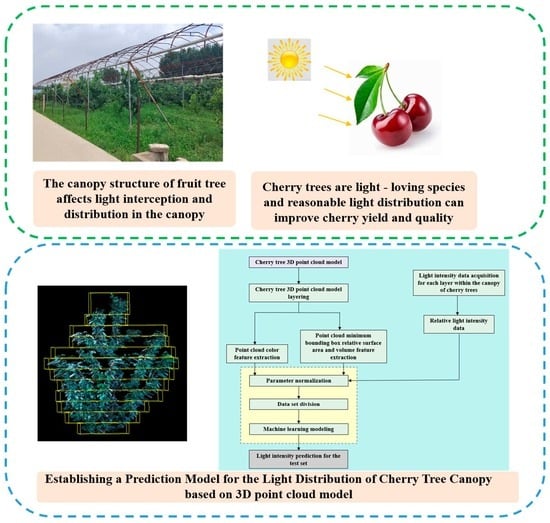
2.4.1. Light Distribution Prediction Method Flow

The flow of our proposed method for predicting the canopy light distribution of cherry trees based on a 3D point cloud model is shown in Figure 7. Based on the above aligned 3D cherry tree point cloud model, we took the point cloud relative projected area features and the relative surface area and volume features of the minimum bounding box as inputs.

2.4.2. Point Cloud Layering

To extract the point cloud features corresponding to different height layers in the cherry tree point cloud model, it was necessary to carry out point cloud stratification of the cherry tree canopy point cloud model. In order to reveal the relationship between cherry tree canopy structure and light distribution, we stratified the canopy point cloud model every 15 cm from bottom to top in the vertical direction based on the light data collection experiment described in Section 2.2.3. If the top layer is less than 15 cm, it will not be layered and, if it exceeds 15 cm, it will also be classified as the first layer. The cherry tree point cloud layering result is shown in Figure 8.

2.4.3. Point Cloud Relative Projection Area Feature Extraction

The projection of the 3D point cloud in the plane of each layer of the cherry canopy possesses morphological self-similarity and similarity to the whole but is not precisely similar. Therefore, within the canopy scale, the 3D point cloud projection of different layers has significant fractal characteristics. The point cloud relative projection area calculation method is described as follows.

First, we performed a horizontal projection of the layered cherry canopy layer point cloud model, as shown in Figure 9a. To ensure the 2D point cloud quality after projection, we calculated the maximum and minimum values of all points’ z-values in the point cloud to be projected in the coordinate axis, and then replaced the z-values of all points with the average value to achieve the projection of all points onto the same 2D plane.

Then, we used a Graham-scan-based convex hull algorithm [38] and alpha-shapes-based concave hull algorithm [39] to extract the boundary points of horizontal projection of each layer of the point cloud. The results of the convex hull sets and the concave hull sets of the projected region are shown in Figure 9b,c, respectively. It can be found that compared with the convex hull extraction algorithm, the concave hull sets basically coincided with the projected region boundary points. Therefore, we chose the alpha-shapes-based concave hull algorithm to obtain the projected region boundary points.

Finally, the area of the projection region enclosed by the concave hull sets was calculated using vector product fork multiplication.

The projected area of the complete cherry tree canopy point cloud model was regarded as a reference, and the ratio of the projected area of each layer to the reference projected area was considered the relative projected area value. The number of concave hull sets and the relative projected area value in a layered cherry tree canopy point cloud model were measured, and the results are shown in

Table 3. The number of concave hull sets and the relative projected area value in a layered cherry tree canopy point cloud model.

Number of Point Cloud Layers	Number of Points in Concave Hull Sets	Projected Area/m2	Relative Projected Area/m2
1	134	0.1206	0.1057
2	226	0.1062	0.0931
3	325	0.1578	0.1383
4	377	0.2444	0.2142
5	419	0.6706	0.5876
6	402	0.2803	0.2456
7	389	0.5473	0.4796
8	295	0.4316	0.3782
9	212	0.3131	0.2743
10	188	0.0895	0.0784
11	91	0.0047	0.0041
12	79	0.066	5.806
total	360	1.14125	1

.

2.4.4. Point Cloud Minimum Bounding Box Feature Extraction

A bounding box is an algorithm for solving the optimal wraparound space of a discrete point set. The basic idea is to approximate complex geometric objects by replacing them with slightly larger geometries with simple features, which have a wide range of applications, such as mechanical collision testing, object identification and localization [40]. The commonly used algorithms for solving point cloud bounding boxes are the axis-aligned bounding box (AABB) algorithm and the oriented bounding box (OBB) algorithm. Since the AABB algorithm is easily influenced by the orientation of the object and has a large gap with the point cloud data, we used the OBB-based algorithm to extract the minimum enclosing box of the point cloud, treating the surface area and volume of the minimum bounding box as features.

The algorithm is based on the following steps: firstly, all points in the point cloud data are deaveraged and the covariance matrix of the point cloud data is constructed. The three principal axes of the point cloud data are obtained by principal component analysis to construct a new feature space Ω. Then, the original point cloud data are projected into Ω-space to find the minimum and maximum points of the projected data in the three axes. Finally, a bounding box is constructed for the six maximum points in Ω-space and the minimum bounding box of the original data along the principal direction is obtained by reprojecting the coordinates of this box under the original coordinate system. Taking a cherry tree point cloud model as an example, the minimum bounding box is extracted as shown in Figure 10. The surface area of this minimum bounding box is 20.247 m² and the volume is 6.035 m³.

The above algorithm is used to extract the minimum bounding box for each layer of the cherry canopy layer point cloud data and to calculate the surface area and volume characteristics of the minimum enclosing box. The relative surface area and volume of the minimum enclosing box were calculated using Equations (12) and (13), respectively.

$${RArea}_i=\frac{{Area}_i}{TArea}\times 100\%$$

(12)

where ${RArea}_i$ are the relative surface area of the minimum bounding box in layer $i$, ${Area}_i$ is the surface area of the minimum bounding box in layer $i$, $TArea$ is the baseline surface area.

$${RVolume}_i=\frac{{volume}_i}{TVolume}\times 100\%$$

(13)

where ${RVolume}_i$ is the relative surface volume of the minimum bounding box in layer $i$, ${vloume}_i$ is the surface volume of the minimum bounding box in layer $i$, $TVolume$ is the baseline surface volume.

Using a cherry tree canopy point cloud model as an example, the relative surface area and volume of the minimum bounding box for each layer of the point cloud in this model are calculated and the results are shown in

Table 4. Result of the relative surface area and relative volume of the minimum bounding box for each layer of the point cloud.

Number of Point Cloud Layers	Relative Surface Area of the Minimum Bounding Box/m2	Relative Volume of the Minimum Bounding Box/ m3
1	0.064	0.012
2	0.120	0.024
3	0.162	0.033
4	0.214	0.049
5	0262	0.058
6	0.236	0.05
7	0.267	0.06
8	0.25	0.059
9	0.125	0.025
10	0.098	0.021
11	0.038	0.007
12	0.05	0.01
total	1	1

.

2.5. Performance Evaluation

2.5.1. Evaluation of the Point Cloud Data Preprocessing Result

A large amount of background noise and outlier noise in the original cherry tree point cloud data will result in a relatively scattered distribution of all the points in the point cloud data. The point cloud dispersion (dis) was calculated using Equation (14) and used as the evaluation index of the point cloud preprocessing effect.

$${dis}_i={\left(x_i-c_x\right)}^2+{\left(y_i-c_y\right)}^2+{(z_i-c_z)}^2$$

(14)

where $(x_i,y_i,z_i)$ are the point coordinates and $\left(c_x,c_y,c_z\right)$ are the coordinates of the 3D spatial origin.

2.5.2. Evaluation of the Point Cloud Data Registration Result

The root mean square error ($RMSE$) was used to evaluate the effectiveness of the point cloud alignment. The $RMSE$ was calculated using Equation (15).

$$RMSE=\sqrt{\frac{\sum _{i=1}^n{(p_{xi}-q_{xi})}^2+{(p_{yi}-q_{yi})}^2+{(p_{zi}-q_{zi})}^2}{n}}$$

(15)

where $n$ is the number of point clouds, $(p_{xi},p_{yi},p_{zi})$ are the coordinates of the points in the source point cloud and $(q_{xi},q_{yi},q_{zi})$ are the coordinates of the points in the target point cloud.

2.5.3. Evaluation of the Canopy Light Distribution Prediction Method

The R squared ($R^2$) and mean absolute percentage error ($MAPE$) were used to evaluate the light intensity prediction model accuracy. The $R^2$ and $MSE$ were calculated using Equations (16) and (17), respectively.

$$R^2=1-\frac{\sum _{i=1}^n{(\widehat{y_i}-y_i)}^2}{\sum _{i=1}^n{(\stackrel{-}{y_i}-y_i)}^2}$$

(16)

$$MAPE=\frac{1}{n}\sum _{i=1}^n\left|\frac{\widehat{y_i}-y_i}{y_i}\right|$$

(17)

where $n$ is the number of data, $y_i$ is the true value, $\widehat{y_i}$ is the predicted value and $\stackrel{-}{y_i}$ is the sample mean.

3. Results

3.1. Analysis of Point Cloud Preprocessing Results

To verify the effect of point cloud preprocessing, the point cloud dispersion ($Dis$) was calculated for a piece of original cherry tree point cloud data and the preprocessed cherry tree point cloud data, and the results are shown in Figure 11. Before point cloud preprocessing, the maximum point cloud dispersion was 7.45 m, the maximum dispersion difference was 6.63 m and the average dispersion was 2.74 m. After point cloud preprocessing, the maximum point cloud dispersion was reduced to 3.15 m, the maximum dispersion difference was reduced to 1.27 m and the average dispersion was reduced to 2.38 m. This indicated that point cloud preprocessing contributed to a more concentrated point cloud distribution.

3.2. Analysis of Cherry Tree Point Cloud Alignment Accuracy

In this experiment, four cherry trees of different shapes in the cherry orchard were selected as the experimental objects. The point cloud data of cherry trees in the leaf curtain stabilization period and dormant period were collected in two stations using the vision system we built and the point cloud was coarsely and precisely aligned. The point cloud alignment process of the cherry trees in the leaf curtain stabilization period is shown in Figure 12, and the point cloud alignment process of the cherry trees in the dormant period is shown in Figure 13.

The point cloud data of four cherry trees were coarsely and precisely aligned, and the alignment time and alignment error were measured. The results of the point cloud alignment of cherry trees in the leaf curtain stabilization period are shown in

Table 5. Result of the point cloud alignment of cherry trees during leaf curtain stabilization period.

Cherry Tree Number	Coarse Alignment		Precise Alignment
	Time/s	RMSE/cm	Time/s	RMSE/cm
1	11.178	0.998	3.103	0.679
2	13.747	1.154	4.204	0.662
3	10.645	1.085	4.228	0.628
4	14.752	1.128	5.227	0.712

, and the results of the point cloud alignment of cherry trees in the dormant period are shown in

Table 6. Result of the point cloud alignment of cherry trees during dormant period.

Cherry Tree Number	Coarse Alignment		Precise Alignment
	Time/s	RMSE/cm	Time/s	RMSE/cm
1	4.523	0.935	2.598	0.520
2	3.941	0.700	2.637	0.498
3	3.301	0.782	4.228	0.435
4	5.148	0.887	5.227	0.582

.

Analysis of the experimental data in the above tables showed that the coarse alignment of the point cloud resulted in a better initial position of the two cherry tree point clouds. However, there was still a certain amount of alignment error, which was further reduced by the fine alignment method. In terms of alignment time, the coarse alignment took longer because it involved the extraction of ISS key points from the cherry tree point cloud data. Dormant cherry trees did not contain leaves and had a relatively simpler morphological structure than cherry trees in the leaf curtain stabilization period, so the point cloud alignment time was shorter and the alignment error was smaller.

3.3. Analysis of Cherry Tree Canopy Light Distribution Prediction Method

The experiments were validated in a Windows 10 environment with the Anaconda integrated development environment and the TensorFlow development framework based on the Python 3.7 environment. The sklearn library was used to realize the model build and prediction. The Numpy, Scipy and Pandas scientific computing libraries provided in Python were used in the experiments.

3.3.1. Dataset Construction

Taking a cherry tree as an example, its corresponding cherry tree point cloud canopy model was layered every 15 cm in the vertical direction, which could be cut into 12 layers. Using the feature extraction method proposed in Section 2.4, the three features corresponding to the relative projected area, the relative surface area and volume of the minimum bounding box of the point cloud were calculated for each layer as the model input data. Based on the canopy light data collection experiments described in Section 2.2.3, the relative light intensity was calculated for a total of 432 collected light data and used as the model output value. Following the method described above, the data were processed for the three selected cherry trees to obtain a total of 1332 sets of data, which would form the dataset. The dataset was randomly divided into a training set and a test set at a ratio of 7.5:2.5, and random number seeds were set to control the variables to compare the prediction results. The data in the training and validation sets were normalized using a feature engineering normalization function to remove the effect of data magnitude on the prediction results.

3.3.2. Predictive Model Selection

To find the optimal prediction model, multiple regression algorithms were selected to predict the light distribution pattern in the canopy layer of the cherry tree population. Using the relative projected area, the relative surface area and volume of the minimum bounding box characteristics as independent variables and the relative light intensity values as dependent variables, the linear regression (LR) and support vector regression (SVR) classical regression methods and the adaptive boosting (AdaBoost) and gradient boost regression tree (GBRT) [41] integrated regression algorithms were used to perform regression analysis on the data.

The regression models were analyzed for prediction accuracy through the validation set data. The $R^2$ and MAPE were selected as accuracy evaluation indicators. The comparison of the relative light intensity prediction results of the different models with the real results is shown in Figure 14. A comparison of the regression accuracy of the different models is shown in

Table 7. Regression accuracy comparison between different models.

Model	${\mathit{R}}^2$	$\mathit{M}\mathit{A}\mathit{P}\mathit{E}$
LR	0.041	0.567
SVR	0.049	0.554
AdaBoost	0.715	0.265
GBRT	0.932	0.116

.

The regression accuracies of the classical regression models were all lower than those of the integrated regression models, with the GBRT model having the best regression accuracy and the LR model having the worst. The LR model had the lowest prediction accuracy because it only required a minimum loss function rather than a good fit of the data in terms of optimization parameters. The low prediction accuracy of the SVR model was due to the vulnerability of the model to neighborhood data. As the feature extraction in this study was mainly for the point cloud data of the canopy layer of cherry trees after stratification, the neighboring point cloud data features had some influence on the model accuracy. In the integrated regression algorithm, the prediction accuracy of the AdaBoost model was lower than that of the GBRT model. This was because the AdaBoost model was sensitive to the anomalous sample values. The anomalous samples may have received higher weights during the iterative process, which eventually affected the prediction accuracy. Therefore, the GBRT model was chosen for the prediction of the cherry tree canopy light distribution.

4. Discussion

4.1. Comparison of Different Alignment Methods

To further verify the generality and effectiveness of the method we propose, eight sets of cherry tree point cloud data were aligned using the SIFT-ICP algorithm [42], ISS-NDT algorithm [43], ISS-ICP algorithm and the ISS-bi-KD-tree-ICP algorithm proposed in this paper. The average alignment time and average alignment error of the above alignment algorithms are shown in

Table 8. Results of different alignment methods.

Alignment Method	Time/s	RMSE/cm
SIFT-ICP	15.827	0.982
ISS-NDT	12.528	0.728
ISS-ICP	13.429	0.694
ISS-bi-KD-tree-ICP	11.835	0.589

.

Analysis of the data in the above table shows that the alignment time of the ICP algorithm is longer than that of the NDT algorithm, but the alignment accuracy is higher. Compared with the SIFT-ICP algorithm, the alignment time and alignment error of the ISS-ICP algorithm were both less, indicating that the key points extracted by the ISS-ICP algorithm could describe the local features of the point cloud to a greater extent and were more stable for the cherry tree point cloud data. Compared with the ISS-ICP algorithm, the ISS-bi-KD-tree-ICP algorithm proposed in this paper was less time consuming. This was because the ICP algorithm was not efficient in computing the nearest points between two point clouds after coarse alignment because of the one-to-many situation, while the improved ICP algorithm based on a bidirectional KD-tree could perform the calculation more quickly. The bi-KD-tree-ICP algorithm could calculate the nearest points between the two point clouds after coarse alignment more quickly and accurately, thus improving the alignment efficiency. According to the above comparative analysis, the time complexity of the alignment method proposed in this paper has been greatly reduced and the alignment accuracy has been significantly improved.

4.2. Effect of Different Point Cloud Feature Choices on Model Prediction Results

In order to investigate the influence of different feature combinations on the accuracy of cherry tree canopy light distribution prediction models, three feature selection schemes were designed in this study, as shown in

Table 9. Feature combination schemes and results.

Feature Combination Schemes	Feature Combination Results
Scheme 1	Relative projection area
Scheme 2	Relative surface area and volume of the minimum bounding box
Scheme 3	Relative projection area, relative surface area and volume of the minimum enclosing box

. The regression analysis of the three feature combination schemes was carried out using the GBRT model. The comparison results of the prediction accuracy are shown in

Table 10. Comparison of prediction accuracy of different feature combinations.

Feature Combination Schemes	${\mathit{R}}^2$	$\mathit{M}\mathit{A}\mathit{P}\mathit{E}$
Scheme 1	0.919	0.136
Scheme 2	0.915	0.137
Scheme 3	0.932	0.116

. The analysis showed that the regression accuracy of feature selection scheme 3 was the highest. Therefore, we constructed a GBRT model based on the relative projection area, the relative surface area and volume of the minimum bounding box of point clouds as the feature inputs and the relative light intensity as the output, to build ad prediction model for the light distribution in the cherry canopy layer.

5. Conclusions

To reveal the pattern between the canopy structure of fruit trees and the light distribution, we took cherry trees as the experimental object and fused the cherry tree point cloud data collected from multiple sources to establish a complete 3D cherry tree point cloud model. This was used to construct a prediction model of the light distribution in the canopy of cherry trees. Some specific conclusions drawn from this study included the following:

(1)

A visual system based on a binocular depth camera was built. Using this visual system to scan a cherry tree from both front and rear stations, complete color point cloud data of the cherry tree could be obtained quickly and accurately.

(2)

A global alignment method is proposed for the point cloud data of cherry trees based on the visual system we developed. Four randomly selected cherry trees in the cherry orchard were used as experimental objects. The ICP algorithm, SIFT-ICP algorithm, ISS-ICP algorithm and global alignment method proposed in this paper were compared and analyzed. The average time taken for the global alignment method proposed in this paper was 11.835 s, and the $RMSE$ was 0.589 cm, which show effectively reduced alignment time and alignment error.

(3)

A method for quantifying the canopy structure of cherry trees is proposed. Firstly, the cherry tree point cloud model is stratified. Secondly, the point cloud projected area features are calculated using an alpha-shapes-based concave wrapping algorithm. The surface area and volume features of the minimum bounding box of the point cloud are calculated using the OBB-based minimum bounding box extraction algorithm. Finally, structural quantification of different areas of the cherry tree canopy is implemented in two dimensions and three dimensions.

(4)

A GBRT-based light prediction model for cherry tree canopies is proposed, which takes point cloud relative projected area features and the relative surface area and volume features of the minimum bounding box as inputs and the relative light intensity as output. The experimental results showed that the $R^2$ and $MAPE$ between the predicted and actual values were 0.932 and 0.16, respectively. The model could more accurately predict the light distribution within the canopy of cherry trees.

Future research will focus on 3D reconstruction and branch identification of dormant cherry trees to provide technical support for rational optimization of the canopy structure and automated pruning of cherry trees.

References

1. Amatya, S.; Karkee, M.; Gongal, A.; Zhang, Q.; Whiting, M.D. Detection of cherry tree branches with full foliage in planar architecture for automated sweet-cherry harvesting. Biosyst. Eng. 2016, 144, 3–15. [Google Scholar] [CrossRef]
2. Wilkie, J.D.; Conway, J.; Griffin, J.; Toegel, H. Relationships between canopy size, light interception and productivity in conventional avocado planting systems. J. Hortic. Sci. Biotechnol. 2019, 94, 481–487. [Google Scholar] [CrossRef]
3. Chen, M.; Tang, Y.; Zou, X.; Huang, K.; Huang, Z.; Zhou, H.; Wang, C.; Lian, G. Three-dimensional perception of orchard banana central stock enhanced by adaptive multi-vision technology. Comput. Electron. Agric. 2020, 174, 105508. [Google Scholar] [CrossRef]
4. Westling, F.; Underwood, J.; Örn, S. Light interception modelling using unstructured LiDAR data in avocado orchards. Comput. Electron. Agric. 2018, 153, 177–187. [Google Scholar] [CrossRef]
5. Kolmanič, S.; Strnad, D.; Kohek, Š.; Benes, B.; Hirst, P.; Žalik, B. An algorithm for automatic dormant tree pruning. Appl. Soft Comput. 2020, 99, 106931. [Google Scholar] [CrossRef]
6. Long, H.; James, S. Sensing and Automation in Pruning of Apple Trees: A Review. Agronomy 2018, 8, 211. [Google Scholar]
7. Azlan, Z.; Sultan, M.M.; Long, H.; Paul, H.; Daeun, C.; James, S. Technological advancements towards developing a robotic pruner for apple trees: A review. Comput. Electron. Agric. 2021, 189, 106383. [Google Scholar]
8. Yang, W.; Chen, X.; Saudreau, M.; Zhang, X.; Zhang, M.; Liu, H.; Costes, E.; Han, M. Canopy structure and light interception partitioning among shoots estimated from virtual trees: Comparison between apple cultivars grown on different interstocks on the Chinese Loess Plateau. Trees 2016, 30, 1723–1734. [Google Scholar] [CrossRef]
9. Weiwei, Y.; Chen, X.; Zhang, M.; Gao, C.; Liu, H.; Saudreau, M.; Costes, E.; Han, M. Light interception characteristics estimated from three-dimensional virtual plants for two apple cultivars and influenced by combinations of rootstocks and tree architecture in Loess Plateau of China. Acta Hortic. 2017, 1160, 245–252. [Google Scholar]
10. Rengarajan, R.; Schott, J.R. Modeling and Simulation of Deciduous Forest Canopy and Its Anisotropic Reflectance Properties Using the Digital Image and Remote Sensing Image Generation (DIRSIG) Tool. IEEE J. Stars. 2017, 10, 4805–4817. [Google Scholar] [CrossRef]
11. Chelle, M.; Andrieu, B. The nested radiosity model for the distribution of light within plant canopies. Ecol. Model. 1998, 111, 75–91. [Google Scholar] [CrossRef]
12. Jean, D.; Pascal, C.; Delphine, L.; Pierre, M. Using virtual plants to analyse the light-foraging efficiency of a low-density cotton crop. Ann. Bot. 2008, 101, 1153–1166. [Google Scholar]
13. Zheng, C.; Wen, W.; Lu, X. Phenotypic traits extraction of wheat plants using 3D digitization. Smart Agric. 2022, 4, 150–162. [Google Scholar]
14. Jaewoo, K.; Hyun, K.W.; Eek, S.J. Interpretation and Evaluation of Electrical Lighting in Plant Factories with Ray-Tracing Simulation and 3D Plant Modeling. Agronomy 2020, 10, 1545. [Google Scholar]
15. Binglin, Z.; Fusang, L.; Ziwen, X.; Yan, G.; Baoguo, L.; Yuntao, M. Quantification of light interception within image-based 3D reconstruction of sole and intercropped canopies over the entire growth season. Ann. Bot. 2020, 126, 701–712. [Google Scholar]
16. Li, S.; Zhu, J.; Evers, J. Estimating the differences of light capture between rows based on functional-structural plant model in simultaneous Maize-Soybean strip intercropping. Smart Agric. 2022, 4, 97–109. [Google Scholar]
17. Ma, X.; Guo, C.; Zhang, X.; Ma, L.; Zhang, L.; Liu, G. Calculation of Light Distribution of Apple Tree Canopy Based on Color Characteristics of 3D Point Cloud. Trans. Chin. Soc. Agric. Mach. 2015, 46, 263–268. [Google Scholar] [CrossRef]
18. Guo, C.; Zhang, W.; Liu, G.; Feng, J. Illumination Spatial Distribution Prediction Method Based on Apple Tree Canopy Box-Counting Dimension. Trans. Chin. Soc. Agric. Eng. 2018, 34, 177–183. [Google Scholar] [CrossRef]
19. Shi, Y.; Geng, N.; Hu, S.; Zhang, Z.; Zhang, J. Illumination Distribution Model of Apple Tree Canopy Based on Random Forest Regression Algorithm. Trans. Chin. Soc. Agric. Mach. 2019, 50, 214–222. [Google Scholar] [CrossRef]
20. Condotta, I.C.F.S.; Brown-Brandl, T.M.; Pitla, S.K.; Stinn, J.P.; Silva-Miranda, K.O. Evaluation of low-cost depth cameras for agricultural applications. Comput. Electron. Agr. 2020, 173, 105394. [Google Scholar] [CrossRef]
21. Li, Z.; Guo, R.; Li, M.; Chen, Y.; Li, G. A review of computer vision technologies for plant phenotyping. Comput. Electron. Agr. 2020, 176, 105672. [Google Scholar] [CrossRef]
22. Rincón, M.G.; Mendez, D.; Colorado, J.D. Four-Dimensional Plant Phenotyping Model Integrating Low-Density LiDAR Data and Multispectral Images. Remote Sens. 2022, 14, 356. [Google Scholar] [CrossRef]
23. Lambertini, A.; Mandanici, E.; Tini, M.A.; Vittuari, L. Technical Challenges for Multi-Temporal and Multi-Sensor Image Processing Surveyed by UAV for Mapping and Monitoring in Precision Agriculture. Remote Sens. 2022, 14, 4954. [Google Scholar] [CrossRef]
24. Zheng, L.; Wang, L.; Wang, M.; Ji, R. Automated 3D Reconstruction of Leaf Lettuce Based on Kinect Camera. Trans. Chin. Soc. Agric. Mach. 2021, 52, 159–168. [Google Scholar] [CrossRef]
25. Guo, C.; Liu, G.; Zhang, W.; Feng, J. Apple tree canopy leaf spatial location automated extraction based on point cloud data. Comput. Electron. Agr. 2019, 166, 104975. [Google Scholar] [CrossRef]
26. Qi, W.; Qin, Z. Three-Dimensional Reconstruction of a Dormant Tree Using RGB-D Cameras. In Proceedings of the 2013 American Society of Agricultural and Biological Engineers Annual International Meeting, Kansas, MO, USA, 21–24 July 2013. [Google Scholar]
27. Ma, B.; Du, J.; Wang, L.; Jiang, H.; Zhou, M. Automatic branch detection of jujube trees based on 3D reconstruction for dormant pruning using the deep learning-based method. Comput. Electron. Agric. 2021, 190, 106484. [Google Scholar] [CrossRef]
28. Besl, P.J.; McKay, N.D. A method for registration of 3-D shapes. In Proceedings of the Sensor Fusion IV: Control Paradigms and Data Structures, Boston, MA, USA, 14–15 November 1991. [Google Scholar]
29. Saarinen, J.; Andreasson, H.; Stoyanov, T.; Lilienthal, A.J. Normal distributions transform Monte-Carlo localization (NDT-MCL). In Proceedings of the IEEE/RSJ International Conference on Intelligent Robots and Systems (IROS), Tokyo, Japan, 3–7 November 2013. [Google Scholar]
30. Du, S.; Liu, J.; Zhang, C.; Zhu, J.; Ke, L. Probability iterative closest point algorithm for m-D point set registration with noise. Neurocomputing 2015, 157, 187–198. [Google Scholar] [CrossRef]
31. Du, S.; Xu, G.; Zhang, S.; Zhang, X.; Gao, Y.; Chen, B. Robust rigid registration algorithm based on pointwise correspondence and correntropy. Pattern Recogn. Lett. 2020, 132, 91–98. [Google Scholar] [CrossRef]
32. Yan, J.; Shan, J.; Jiang, W. A global optimization approach to roof segmentation from airborne lidar point clouds. ISPRS J. Photogramm. 2014, 94, 183–193. [Google Scholar] [CrossRef]
33. Xijiang, C.; Hao, W.; Derek, L.; Xianquan, H.; Ya, B.; Peng, L.; Hui, D. Extraction of indoor objects based on the ex-ponential function density clustering model. Inform. Sci. 2022, 607, 1111–1135. [Google Scholar]
34. Yusheng, X.; Wei, Y.; Sebastian, T.; Ludwig, H.; Uwe, S. Unsupervised Segmentation of Point Clouds from Buildings Using Hierarchical Clustering Based on Gestalt Principles. IEEE J. Stars. 2018, 11, 4270–4286. [Google Scholar]
35. Guichao, L.; Yunchao, T.; Xiangjun, Z.; Chenglin, W. Three-dimensional reconstruction of guava fruits and branches using instance segmentation and geometry analysis. Comput. Electron. Agric. 2021, 184, 106107. [Google Scholar]
36. Rusu, R.B.; Cousins, S. 3D is here: Point Cloud Library (PCL). In Proceedings of the IEEE International Conference on Robotics & Automation, Shanghai, China, 9–13 May 2011. [Google Scholar]
37. Liu, W.; Xie, Y.; Chen, R. Observation of relationship between zenith luminance and sun high angle. Opto-Electron. Eng. 2012, 39, 49–54. [Google Scholar]
38. Liu, R.; Tang, Y.Y.; Fang, B.; Pi, J. An enhanced version and an incremental learning version of visual-attention-imitation convex hull algorithm. Neurocomputing 2014, 133, 231–236. [Google Scholar] [CrossRef]
39. Zheng, Y. Canopy Parameter Estimation of Citrus grandis var. Longanyou Based on LiDAR 3D Point Clouds. Remote Sens. 2021, 13, 1859. [Google Scholar]
40. Ji, Y.; Li, S.; Peng, C.; Xu, H.; Cao, R.; Zhang, M. Obstacle detection and recognition in farmland based on fusion point cloud data. Comput. Electron. Agric. 2021, 189, 106409. [Google Scholar] [CrossRef]
41. Xinkai, C.; Ni, R.; Ganglu, T.; Yuxing, F.; Qingling, D. A three-dimensional prediction method of dissolved oxygen in pond culture based on Attention-GRU-GBRT. Comput. Electron. Agric. 2021, 181, 105955. [Google Scholar]
42. Scovanner, P.; Ali, S.; Shah, M. A 3-dimensional sift descriptor and its application to action recognition. In Proceedings of the 15th International Conference on Multimedia 2007, Augsburg, Germany, 24–29 September 2007. [Google Scholar]
43. Zhu, T.; Ma, X.; Guan, H.; Wu, X.; Wang, F.; Yang, C.; Jiang, Q. A calculation method of phenotypic traits based on three-dimensional reconstruction of tomato canopy. Comput. Electron. Agric. 2023, 204, 107515. [Google Scholar] [CrossRef]
Figure 1. (a) Cherry orchard trial plots; (b) 3D data acquisition platform: (1) Azure Kinect DK cameras; (2) camera mounts; (3) mobile power; (4) portable computer; (5) target balls; (6) engineering lighting.
Remotesensing 15 02516 g001
Figure 2. (a) Schematic diagram of cherry tree point cloud data collection; (b) 3D information data of cherry trees acquired using the DK cameras.
Remotesensing 15 02516 g002
Figure 3. (a) Original cherry tree point cloud data; (b) effect picture after background noise removal; (c) effect picture after outlier removal; (d) effect picture after point cloud downsampling.
Remotesensing 15 02516 g003
Figure 4. Light data collection.
Remotesensing 15 02516 g004
Figure 5. Overall flow chart of the global alignment.
Remotesensing 15 02516 g005
Figure 6. (a) Cherry tree point cloud data after preprocessing; (b) ISS key points in cherry tree point cloud data.
Remotesensing 15 02516 g006
Figure 7. Light distribution prediction method flow.
Remotesensing 15 02516 g007
Figure 8. Cherry tree canopy point cloud layering result.
Remotesensing 15 02516 g008
Figure 9. (a) Cherry tree point cloud projection; (b) convex hull sets of the projected region; (c) concave hull sets of the projected region.
Remotesensing 15 02516 g009
Figure 10. Extraction result of the minimum bounding box for cherry tree point cloud data.
Remotesensing 15 02516 g010
Figure 11. (a) Point cloud dispersion plot before preprocessing; (b) point cloud dispersion plot after preprocessing.
Remotesensing 15 02516 g011
Figure 12. Point cloud alignment process on cherry trees during leaf curtain stabilization period.
Remotesensing 15 02516 g012
Figure 13. Point cloud alignment process on cherry trees during dormant period.
Remotesensing 15 02516 g013
Figure 14. (a) LR; (b) SVR; (c) AdaBoost; (d) GBRT.
Remotesensing 15 02516 g014aRemotesensing 15 02516 g014b