Monitoring the Degree of Mosaic Disease in Apple Leaves Using Hyperspectral Images

Abstract

Mosaic of apple leaves is a major disease that reduces the yield and quality of apples, and monitoring for the disease allows for its timely control. However, few studies have investigated the status of apple pests and diseases, especially mosaic diseases, using hyperspectral imaging technology. Here, hyperspectral images of healthy and infected apple leaves were obtained using a near-ground imaging high spectrometer and the anthocyanin content was measured simultaneously. The spectral differences between the healthy and infected leaves were analyzed. The content of anthocyanin in the leaves was estimated by the optimal model to determine the degree of apple mosaic disease. The leaves exhibited stronger reflectance at a range of 500–560 nm as the degree of disease increased. The correlation between the spectral reflectance processed by the Gaussian1 wavelet transform and anthocyanin was significantly improved compared to the corresponding correlation results with the original spectrum. The VPs-XGBoost anthocyanin estimation model performed the best, which was sufficient to monitor the degree of the disease. The findings provide theoretical support for the quantitative estimation of leaf anthocyanin content by remote sensing to monitor the degree of disease; they lay the foundation for large-scale monitoring of the degree of apple mosaic disease by remote sensing.

1. Introduction

Apple trees, belonging to the rose family, are one of the most widely cultivated fruit trees in the world, and the fruits have high nutritional value and great economic benefits. China is the world’s largest apple producer, accounting for 50% of the global apple production in recent years [1]. Mosaic is a common viral disease that occurs during the growth of apple trees and is characterized by strong infectivity, fast transmission, and wide distribution. Mosaic disease may cause serious yield loss [2,3]. Apple leaves infected with mosaic virus show chlorotic (yellow) spots or mosaic patterns that develop along the veins or form amorphous chlorosis zones between veins [4].

Anthocyanins are one of the main pigments in plants and usually exist in the cytoplasm. As an osmoregulatory substance, anthocyanins—with their unique antioxidant effect—protect the photosynthetic system of plants from excessive light radiation, especially ultraviolet radiation [5,6]. Anthocyanin is also a secondary metabolite of plants subjected to environmental and biological stresses such as high temperature, water shortage, high salt, diseases, and insect pests. Studies have shown that anthocyanin concentrations increase significantly when plants are subjected to biological or abiotic stresses [7]. Therefore, dynamic information on the anthocyanin content in apple leaves can serve as an important basis for judging the degree of leaf disease.

However, traditional methods for measuring the anthocyanin content in vegetation can be destructive, time-consuming, and laborious, rendering them difficult to implement in agricultural production [8,9,10]. Therefore, it is necessary to develop an effective and nondestructive method to estimate the anthocyanin content. Hyperspectral imaging is an extensive and automated measurement technology that can capture the fine spectral data of plants and provide nondestructive and real-time monitoring of aspects of crops such as nutrient, disease, and insect status [11,12,13]. Based on the hyperspectral data, scholars have proposed a number of spectral pretreatment methods and hyperspectral vegetation indices including the Savitzky–Golay smoothing method (S–G smoothing), successive projections algorithm (SPA), red-edge parameter, and new vegetation indices, which are usually used to detect diseases and pigment content and monitor physiological and biochemical parameters and growth information in crops and vegetation [14,15,16,17,18,19]. Liu found that S–G smoothing is an ideal method for reducing noise when exploring the application status of NDVI time series data [20]. Ruffion believed that the spectrum after S–G smoothing was more conducive to the subsequent extraction of the spectral characteristics of plants and soil [21]. Wang (2016) suggested that the performance of the three-band vegetation index constructed based on the wavelength selected by SPA was higher than that selected by the genetic algorithm, indicating that SPA has great potential in crop monitoring [22]. The study by Ding (2022) showed that SPA-ELM can quickly and accurately evaluate the chlorophyll content and hardness of cucumber [23]. Gitelson believed that the 510–560 nm and near-infrared bands could accurately and nondestructively estimate the anthocyanin content in plant leaves; however, specific parameters would vary for different types of vegetation [24]. Steele pointed out that the near-infrared/green (AIR) index and improved anthocyanin reflectance index (MARI) are effective tools for estimating the anthocyanin content of grape leaves [9]. Luo established the anthocyanin content of single- and multi-class variable inversion models, and the results showed that the modeling accuracy of the multi-class variable model significantly improved [25]. Other studies have shown that continuous wavelet transform captures more spectral information than the previously used transform methods in the context of vegetation hyperspectral remote sensing [26,27], which also demonstrates the advantages of wavelet transform in spectral smoothing, noise reduction [28,29], classification recognition [26,30,31], and the estimation of the leaf pigment content [32,33].

Hyperspectral imaging is a new nondestructive detection technology that combines traditional imaging technology with spectral technology [34] and has been widely used in monitoring crop diseases and pests in recent years. The captured images have the characteristics of atlas integration, and every pixel in the image contains rich spectral information, which compensates for the limitations of traditional imaging technology and spectral analysis [35]. Zhang combined hyperspectral images with the photochemical reflection index (PRI) to effectively distinguish the degree of disease in wheat yellow rust [36]. Xie identified the early blight of eggplant leaves using a GLCM based on hyperspectral images [37]. Koushik proposed that the preprocessing of hyperspectral images and the extraction of sensitive bands combined with deep learning could classify charcoal rot and thus monitor the health status of soybeans [38]. Gerrit Polder used hyperspectral images instead of visual observation to monitor potato virus diseases in the early cultivation stage, thus reducing the planting cost for farmers [39]. Yuan suggested that the automated and accurate detection of anthracnose-infected tea leaves was possible by using hyperspectral imaging for practical tea-plant protection [40]. Wu combined machine learning algorithms with hyperspectral image features to monitor rice bacterial blight, achieving recognition accuracies as high as 97.41% [41]. The use of hyperspectral data to monitor crop growth or their health consists of two main approaches: standard statistical models and machine learning-based regression models [42]. Tao directly constructed a yield prediction model by analyzing the patterns of the spectral characteristics of crops [43]; Ta used the vegetation index and standard linear estimation to estimate the leaf nitrogen content, but the accuracy was not very good [44] as these statistical models are usually more suitable for data with narrow attributes. The use of regression models based on machine learning greatly improved the speed of data processing and emphasized the effectiveness of the models. Luo believed that partial least square regression (PLSR) and support vector machine regression (SVMR) were significantly better than ordinary linear regression in estimating the anthocyanin content in maize leaves [25]. Wei successfully identified the characteristics of different crops in the early growing stage by combining RF and vegetation index [45].

Most of these studies have focused on the estimation of crop parameters, the classification and identification of crop diseases and pests, while few have investigated the status of apple pests and diseases using hyperspectral imaging technology, especially mosaic diseases. In this study, we applied wavelet transform to the surveillance of apple mosaic disease and proposed comprehensive indicators to estimate the severity of apple mosaic disease for the first time. Therefore, this study aimed to: (1) analyze the spectral characteristics of apple leaves under mosaic stress; (2) compare the inversion performance of characteristic bands, vegetation indices, wavelet coefficients, and effective parameters on anthocyanin, and use the optimal anthocyanin inversion model to obtain a map of leaf anthocyanin content and to evaluate the degree of mosaic disease.

2. Materials and Methods

2.1. Sample Collection and Data Acquisition

The experiment was conducted in June 2021 in an orchard in the Shaozhai Village, Xinglin Town, Fufeng County, Shaanxi Province (Figure 1). During an epidemic of mosaic disease, 180 samples containing healthy apple leaves and leaves with different degrees of disease (based on visual characteristics) were collected and placed in sealed bags. The leaves were placed in an incubator with a built-in ice pack to keep them fresh and then quickly brought back to the laboratory for follow-up measurements.

The anthocyanin content in the apple leaves was measured using a portable plant leaf measuring instrument (Dualex Scientific+, Force-a, Orsay Cedex, France) that uses plant fluorescence technology to achieve real-time, nondestructive, and accurate measurement of anthocyanin content in plant leaves and obtain dimensionless relative values of anthocyanin, namely, the anthocyanin value [23]. Each healthy leaf was measured 10 times (unmeasured veins), and the mean value was denoted as the representative value of anthocyanins. In the infected leaves, measurements were taken only at the diseased spots.

Hyperspectral images of the apple leaves were captured using a SOC-710 portable hyperspectral spectrometer (Surface Optics Corp, San Diego, CA, USA), a hyperspectral spectrometer with built-in translation, a push-and-sweep device, and a dual CCD detector, which can quickly acquire hyperspectral image data at 400–1000 nm with a spectral resolution of 4.7 nm. After measuring the anthocyanin content, apple leaves were placed horizontally on a black curtain with the absorption side up (Figure 1). Hyperspectral images were captured outdoors from 12:00 to 13:30, when the weather was clear with no wind or clouds.

2.2. Data Pre–Processing

2.2.1. Hyperspectral Data Preprocessing

Hyperspectral images were processed using ENVI 5.3 (Exelis, McLean, VA, USA), and the ROI tool was used to draw a region of interest corresponding to the measurement point of the leaf anthocyanin and extract the spectral reflectance. To obtain more spectral information, the spectral reflectance was linear interpolated to a 1 nm resolution from the native 4.7 nm resolution of the instrument following standard practice to standardize the data [33,46]. After removing the outliers, a Savitzky–Golay smoothing method in MATLAB R2021 b (MathWorks, Natick, MA, USA) was used to denoise the spectrum. The quadratic term was set to 5, and a continuous smooth reflection spectrum was finally obtained, which was used as the original spectrum for subsequent research.

2.2.2. Vegetation Indices

Vegetation indices improve the efficiency of data utilization through normalization and derivative processing to reduce the impact of sensors and their surroundings on the measurement target [16,47]. Based on previous experience and knowledge of the characteristic spectral reflectance of apple leaves, this study selected 15 vegetation indices that have good correlations with the pigment content of plants for the analysis of their correlations with the anthocyanin content. Seven three-band vegetation indices and eight two-band vegetation indices were included (

Table 1. Vegetation indices and equations.

Vegetation Indices	Bands	Equation	Reference
NDSI	Any two bands	$\frac{R_i-R_j}{R_i+R_j}$	[48]
RSI		$R_i/R_n$	[48]
DSI		$R_i-R_n$	[48]
TVI	Three specific bands	$0.5(120 \ast \left(R_{750}-R_{550}\right)-200\left(R_{670}-R_{550}\right))$	[14]
VARI		$(R_{550}-R_{660})/(R_{550}+R_{660}-R_{470})$	[45]
MTVI1		$1.2(1.2\left(R_{800}-R_{550}\right)-2.5(R_{670}-R_{550}\left)\right)$	[15]
MCARI1		$1.2\left(2.5\right(R_{800}-R_{670}$$)-1.3(R_{800}-R_{550}$))	[15]
MCARI2		$\frac{1.5 \ast (2.5 \ast \left(R_{800}-R_{670}\right)-1.3 \ast (R_{800}-R_{550}\left)\right)}{\sqrt{{(2 \ast R_{800}+1)}^2-\left(6 \ast R_{800}-5 \ast \sqrt{R_{670}}\right)-0.5}}$	[15]
TCARI		$3[\left(R_{700}-R_{670}\right)-0.2\left(R_{700}-R_{550}\right) \ast (R_{700}/R_{670}\left)\right]$	[40]
MTCI		$(R_{745}-R_{709})/(R_{709}+R_{681})$	[49]
GNDVI	Two specific bands	$\frac{R_{801} - R_{550}}{R_{801} + R_{550}}$	[25]
OSAVI		$\left(1+0.16\right) \ast (R_{800}-R_{670})/(R_{800}+R_{670}+0.16)$	[50]
GRVI		$R_{800}/R_{550}$	[51]
SAVI		$1.5 \ast (R_{800}-R_{670})/(R_{800}+R_{670}+0.5)$	[50]
CARI		$\left(R_{700}-R_{670}\right)-0.2(R_{700}+R_{670})$	[52]

where $R_i$ and $R_j$ are the reflectance at $i$ and $j$ nm over the entire reflectance spectrum, respectively.

). The two-band vegetation indices were further classified into vegetation indices of specific two-band combinations (VI_S) and vegetation indices of any two-band combination (VI_A).

2.3. Variable Selection Methods

2.3.1. Successive Projections Algorithm (SPA)

SPA was originally proposed for the construction of multivariate calibration models, and designed to select variables for use in multiple regression models. In this case, the collinearity avoidance mechanism embedded in the SPA reduced the propagation of measurement noise during calibration [53]. SPA uses the projection analysis of vectors. By projecting the wavelength onto other wavelengths, it compares the size of the projection vector, takes the wavelength with the largest projection vector as the selected wavelength, and then selects the final characteristic wavelength based on the correction model [42]. This study used SPA-GUI for implementation [54], and the steps are described as follows:

Assume that the initial iteration vector is $X_{k\left(0\right)}$, the variable to be extracted is N, and the spectral matrix is J column:

Step 1: One column (the $j$th column) of the spectral matrix was randomly selected, and the $j$th column of the modeling set was assigned to $x_j$, denoted as $X_{k\left(0\right)}$, $j$ = 1, …, $J$;

Step 2: Denoted s as the collection of the column positions that were not selected,

$$\mathrm{s}=\left\{j,1\le j\le Jandj\notin \left\{k\left(0\right),k\left(1\right),\dots \dots ,k\left(n-1\right)\right\}\right\}$$

(1)

Step 3: Compute the projection of $x_j$ onto the remaining column vectors separately,

$$p_{xj}=xj-\left(x_j^T{x}_{k\left(n-1\right)}\right)x_{k\left(n-1\right)}{\left(x_{k\left(n-1\right)}^T{x}_{k\left(n-1\right)}\right)}^{-1}\left(j\in s\right)$$

(2)

Step 4: Extract the spectral wavelength of the maximum projection vector,

$$k\left(n\right)=\mathrm{a}\mathrm{r}\mathrm{g}(\max \left(\parallel p_{xj}\parallel ,j\in s\right)$$

(3)

Step 5: Let

$$x_j=p_{xj},j\in s$$

(4)

Step 6: Accumulate n, if $n<N$, then, it can be calculated in accordance with Equation (1).

Finally, the extracted variable is $\left\{x_{k\left(n\right)}=0,1,\dots ,N-1\right\}.$ Multiple linear regression analysis models were established respectively for $K\left(0\right)$ and $N$ in each cycle, and the root mean square error of the interactive verification of the modeling set was obtained, corresponding to different candidate subsets. According to the F test (α = 0.25), this is the position where RMSE is not significantly greater than the minimum RMSEmin [53].

2.3.2. Continuous Wavelet Transform

Wavelet transform is a linear transformation method that uses wavelet basis functions to decompose complex signals into wavelet signals of different scales or frequencies, effectively extracting weak information parts of the signal, and fully highlighting its local characteristics [55]. Wavelet transform is divided into the continuous wavelet transform (CWT) and discrete wavelet transform. In this study, 10 different parent wavelet bases (

Table 2. Mother wavelet functions and applications.

Mother Wavelet Functions	Applications	Reference
Gaussian 1	Chlorophyll content	[57]
Rbio 5.5	Chlorophyll content	[56]
Mor l	Chlorophyll content	[58]
Db 5	Nitrogen content and classification	[28]
Bior 3.3	Pigment content	[27]
Sym 8	Water content	[59]
Mexh	Water and chlorophyll content	[60]
Meyr	Classification	[29]
Haar	Chlorophyll content	[61]
Coif 2	Chlorophyll content	[62]

) were used to transform the smoothed spectral reflectance into a series of wavelet coefficients. The formulas [56] are given below (Equations (5) and (6)). As wavelet decomposition that occurs on a continuous possible scale ($a$ = 1, 2, …, m) can lead to high computational cost and large data volume, the reflection spectrum was decomposed on a binary scale 2¹, 2², …, 2¹⁰, proportional to the effective length of the wavelet compression or stretching at this scale.

$$\begin{array}{c}Wf\left(a,b\right)={\int }_{-\mathrm{\infty }}^{+\mathrm{\infty }}f\left(\lambda \right){\mathsf{\Psi }}_{a,b}\left(\lambda \right)d\lambda \end{array}$$

(5)

$$\begin{array}{c}{\mathsf{\Psi }}_{a,b}\left(\lambda \right)=\frac{1}{\sqrt{a}}\mathsf{\Psi }\left(\frac{\mathsf{\lambda }-\mathrm{b}}{a}\right)\end{array}$$

(6)

where $Wf\left(a,b\right)$ is the wavelet coefficients; $f\left(\lambda \right)$ is the original hyperspectral reflectance; $\lambda$ is the wavelength; ${\mathsf{\Psi }}_{a,b}\left(\lambda \right)$ is the mother wavelet function; a is the scale factor that defines the width of the wavelet (2¹, 2², …, 2¹⁰); $b$ is the shifting factor determining the position, which shifted from 400 to 988 nm in this study.

The wavelet function provided by MATLAB software in this study was as follows: coefs = cwt (x, scales, ‘wname’), where x is the spectral reflectance of 400–988 nm, scales is a in the above equations, and wname is the mother wavelet function.

2.4. Regression Models

2.4.1. Partial Least-Square Regression (PLSR)

PLSR integrates the advantages of multiple linear regression (MLR), canonical correlation analysis, and principal component analysis (PCA) [63]. In the process of establishing the regression model, the algorithm considers the correlation between the principal component in the feature matrix and the proposed principal component to maximize, which can effectively eliminate multiple correlations among the independent variables and improve the accuracy and overall explanatory ability of the model [64]. In this study, partial least squares regression was used to train the model. The samples were randomly divided into the training group (66.67% of the sample) and the test group (33.33% of the sample). The principal components of different factors were determined by observing the changes in the MSE value of the calibration set after 10-fold cross-validation.

2.4.2. Random Forest (RF) Regression

The RF algorithm is an integrated machine learning algorithm based on the regression tree proposed by Breiman in 2001 [65]. As a bagging integration algorithm with a decision tree as its basic unit, it relies on the assumption that different independently predicted values predict errors in different regions. Therefore, by combining the results of independent predicted values, the overall prediction accuracy can be improved, and it performs well in the training and learning of high-dimensional data such as hyperspectral remote sensing [66,67]. In Python, implemented by the sklearn library, we set the number of trees = 100, the maximum depth of the tree = 8, the number of features of the tree = 5, min_samples_leaf = 1, the number of random seeds = 1, and evaluated using 10-fold cross validation.

2.4.3. Artificial Neural Network (ANN)

The ANN is based on a gradient learning method. It is a nonparametric nonlinear model that uses a neural network layer extension to simulate the human brain receiver and information processing. ANN includes the input, hidden, and output layers, network initialization (i.e., the number of neurons is determined by the input and expected output to initialize the weight between neurons), the hidden layer and output layer calculations, and updating of the error value and weight to obtain the final weight [68]. A neural network is a learning classification method based on large samples, influenced by the network structure and sample complexity, and it is easy to overlearn and reduce its generalization ability. The most important parameter in the neural network regression model is the number of neurons. The greater the number of neurons, the higher the learning accuracy and the stronger the generalization ability [69]. In Python, implemented by the sklearn library, we set the solver = ‘lbfgs’, alpha = 0.001, hidden_layer_sizes = (14, 1), activation = ‘logistic’, learning_rate_init = 0.001, max_iter = 200, and random_state = 600.

2.4.4. Extreme-Gradient Boost (XGBoost) Regression

XGBoost is an enhancement algorithm proposed by Chen in 2016 [70] based on a supervised gradient. In general, the ability of the algorithm to solve a problem is improved by using a custom gradient loss function to improve the framework, which forms new decision trees to constantly fit the residuals of previous predictions to reduce the residual between the actual and predicted values. Compared with previous algorithms, this method controls overfitting better by using a more regularized model. In this study, a tree-based model was used for the lifting calculations. Then, ‘xgboost library’ was imported into Python, class Dmatrix was used to read the data, ‘max_depth’ = 6 was set, eta = 0.1, ‘silent’ = 1, ‘objective’ = ‘reg:squarederror’, ‘subsample’ = 0.5, ‘colsample_bytree’ = 1, ‘min_child_weight’ = 3, num_boost_round = 1000, ‘reg_alpha’ = 0.5, and ‘reg_ lambda = 0.5′.

2.5. Test of Accuracy

We calculated the determination coefficient (R²), root mean square error (RMSE), and relative percentage deviation (RPD). R² is used to evaluate the degree of correlation between the predicted and actual values. The closer R² is to 1, the better the degree of correlation between the predicted and real values. The RMSE is used to test the predictive ability of the model; the smaller the value, the stronger the predictive ability of the model, and the closer the predicted value to the real value. RPD is used to evaluate the stability and prediction ability of the established model. A RPD of less than 1.4 indicates that the model is unstable and has poor prediction ability. A RPD between 1.4 and 2.0 indicates an acceptable model, which can be used for a rough estimation of the target variables and can be improved. When the RPD is 2.0–2.5, the model has good quality and can be used for the quantitative prediction of target variables; when it is greater than 2.5, the model is stable, accurate, and can be used in practice [71].

$$\begin{array}{c}{R}^2=1-\frac{{\sum }_{I=1}^m{\left({\widehat{y}}_i-{\stackrel{-}{y}}_i\right)}^2}{{\sum }_{i=1}^m{\left(y_i-{\stackrel{-}{y}}_i\right)}^2}\end{array}$$

(7)

$$\begin{array}{c}RMSE=\sqrt{\frac{{\sum _{i=1}^m\left(y_i-{\widehat{y}}_i\right)}^2}{m}}\end{array}$$

(8)

$$\begin{array}{c}RPD=\frac{SD}{SEP}\end{array}$$

(9)

where $y_i$ is the measured Anth; ${\widehat{y}}_i$ is the predicted Anth; ${\stackrel{-}{y}}_i$ is the average of measured Anth; $m$ is the number of samples. $SD$ is the standard deviation of the analyzed sample, $SEP$ is the root mean square error of the analyzed sample.

3. Results

3.1. Spectral Characteristics of Leaves

The degree of leaf infection, rated as mild, moderate, and severe, was indicated by a small range of yellow and white spots, large yellow and white spots, and whole-leaf whitening symptoms, respectively. The anthocyanin content was positively correlated with the disease severity (correlation coefficient = 0.784, p < 0.01). The spectral curves of leaves with different degrees of disease (Figure 2) showed that the significant differences were mainly observed in the visible wavelength. With an increase in the degree of disease, the chlorophyll content of the leaves decreased, the photosynthetic capacity of the leaves was relatively weakened, the absorption of red and green light was reduced, and the absorption capacity was significantly enhanced. The stronger reflectance was exhibited at the range of 500–560 nm and the range of 620–640 nm, and an obvious absorption valley was found near 680 nm. For the red edge characteristics, compared with the healthy leaves, the red edge position λ_r showed an obvious phenomenon named “blue shift”.

3.2. Correlation between Spectral Characteristics and Anthocyanin and Select Modeling Parameters

3.2.1. Correlation between Spectral Reflectance and Anthocyanin Content

The correlation between the original spectrum and the leaf anthocyanin content is shown in Figure 3. In the wavelength range of 922–988 nm, the spectral reflectance was significantly negatively correlated with the leaf anthocyanin content, and in the wavelength range of 400–737 nm, the spectral reflectance was significantly positively correlated with the leaf anthocyanin content. Overall, the degree of correlation was higher than that of the NIR above 922 nm, and the correlation coefficient of the 518–602 nm band was above 0.8, with a maximum correlation coefficient of 0.84 at 693 nm. In general, the leaf anthocyanin content was significantly correlated with the spectral reflectance in the visible range, however, in the range of 738–921 nm, it was not significantly correlated, therefore, it is necessary to consider selecting characteristic bands to participate in the modeling.

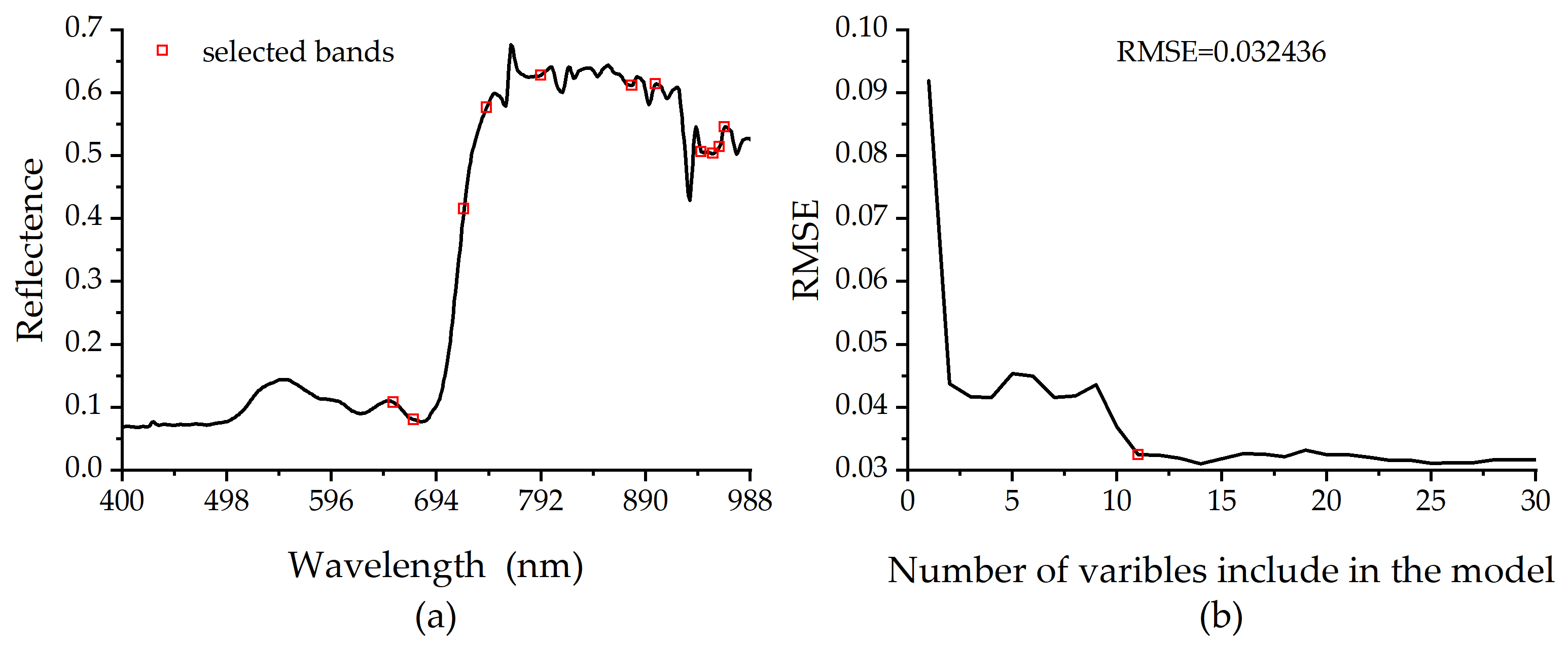
3.2.2. Characteristic Bands Selected by SPA

In this study, we used SPA to select feature wavelengths from high-spectral data that had been smoothed by Savitzky–Golay. Based on the internal cross-validation RMSE, 11 feature bands were obtained: 654 nm, 673 nm, 720 nm, 741 nm, 792 nm, 877 nm, 899 nm, 942 nm, 959 nm, 953 nm, and 964 nm. The positions of the selected wavelengths are shown in Figure 4a. Among them, 654 nm, 673 nm, and 720 nm were located in the interval where the original reflectance was highly correlated with anthocyanin, which is the difference interval of the spectral characteristics between healthy and diseased leaves. The remaining sensitive bands were located at the inflection points of the spectral curve. Therefore, the selected wavelengths contain spectral feature information and reflect the differences between healthy and diseased leaves. After internal cross-validation, they can be used to construct the subsequent anthocyanin estimation model.

3.2.3. Correlation between Vegetation Indices and Anthocyanin Content

The correlation and absolute value of the correlation coefficient (|r|) of various vegetation indices and anthocyanins are shown in

Table 3. R² between the vegetation indices and anthocyanin content.

Vegetation Index	Bands	Coefficient of Determination	Vegetation Index	Bands	Coefficient of Determination
TVI	Three	0.06	MTCI	Three	0.85 **
VARI		0.16 *	GNDVI	Tow	0.90 **
MTVI1		0.05	OSAVI		0.45 **
MCARI1		0.05	GRVI		0.83 **
MCARI2		0.35 **	SAVI		0.77 **
TCARI		0.83 **	CARI		0.46 **

Note: * indicates p < 0.05, ** indicates p < 0.01.

. Except for TVI, MTVI1, and MCARI1, the other vegetation indices were significantly correlated with the leaf anthocyanin content. Among the three-band spectral indices, VARI was significantly correlated with the anthocyanin content at a level of 0.05, and the |r| was the lowest (|r| = 0.06). The others were significantly correlated with the anthocyanin content at a level of 0.01, among which the |r| of MTCI was the highest (|r| = 85), followed by that of TCARI (|r| = 0.83). All two-band vegetation indices were significantly correlated with the anthocyanin content at a level of 0.01, the |r| of which were all greater than 0.45. The GNDVI had the best correlation with the anthocyanin content, with an |r| of 0.90, whereas the GRVI had a weaker correlation with the anthocyanin content (|r| = 0.83).

Figure 5 shows a contour map of the |r| of any two bands combined with the vegetation indices NDSI, RSI, DSI, and the anthocyanin content. The overall results showed that compared with the vegetation indices constructed with the specified band, the whole-band pairwise combination had more advantages in terms of selecting the effective band combinations to construct vegetation indices. The maximum values of the |r| of the three vegetation indices were all greater than 0.90, and the distributions of the |r| of the RSI and NDSI were very similar. Regions with high correlation were mainly located in the combination of near-infrared and green-yellow-red bands, and a small distribution was found in the combination of blue-violet and green bands. However, the ratios were slightly different at 930–980 and 490–690 nm. The overall correlation between the DSI and anthocyanin content was weaker than that between the NDVI and RSI. The figure shows that a high correlation was mainly located in the combinations of 400–500 nm and 490–650 nm. The best combination of each vegetation index was selected according to the correlation level: the correlation between the anthocyanin content and NDSI (at R694, R720) was the best, the highest |r| was 0.922. The |r| of RSI was 0.916, and the corresponding combined wavelengths were R696 and R748. The maximum |r| of the DSI was located at R472 and R580, where the value of |r| was 0.911. In addition, all were significantly correlated according to Pearson’s test.

3.2.4. Correlation between Wavelet Coefficients and Anthocyanin

In MATLAB, the CWT package was used and ten mother wavelet functions were respectively inputted to perform continuous wavelet transform (CWT) on the reflectance curve of the sample points. Then, the correlations between the wavelet coefficients and anthocyanin content were analyzed to obtain the |r| matrix, and an |r| contour map was formed. The overall correlation between the wavelet coefficient obtained by the Gasussian1 transformation and anthocyanin content was the best, with an |r| of up to 0.91. The isoline map of its corresponding |r| is shown in Figure 6, in which the yellow and black blue regions represent strong and weak correlations, respectively.

Figure 6 shows that the correlation between the leaf spectrum after Gaussian1 transformation and anthocyanin content was significantly higher than that of the original spectrum. Among them, the correlation coefficient was the highest at a scale of 6, the sensitive region of anthocyanin was mainly concentrated at 493–543 nm, and the corresponding scales were 5–7, |r|∈(0.89,0.91). This implies that hidden information can be mined effectively using continuous wavelet analysis and by moderately increasing the decomposition scale. In order to deal with the redundancy of wavelet coefficients, after Pearson correlation testing (p > 0.01), the remaining features were arranged in descending order according to |r|, then, a threshold of |r| was applied to delineate the top 2‰ features that were most strongly correlated with the anthocyanin content. Finally, 12 wavelet features were selected.

3.3. Regression Models and Accuracy Evaluation

3.3.1. Models Based on SPA Selected Bands

Characteristic bands screened by the SPA method (λ_spa) were used as input variables of the estimation model. PLSR, RF, ANN, and XGBoost were used to construct an inversion model for apple leaf anthocyanins.

Table 4. Training and validation statistics for the anthocyanin estimation models for λ_spa.

Model	Modeling Set			Verification Set
	R2	RMSEc	RPD	R2	RMSEv	RPD
PLSR	0.713	0.055	1.873	0.828	0.042	2.345
RF	0.965	0.022	4.717	0.736	0.051	1.918
ANN	0.788	0.047	2.183	0.828	0.045	2.196
XGBoost	0.900	0.033	3.124	0.757	0.053	1.865

presents the results. The R² of the λ_spa-PLSR and λ_spa-ANN models was less than 0.8, and the RPD values of the models were low; in particular, the RPD value of the PLSR model was less than 2.0, which implies that the prediction power of the model was poor. In contrast, the modeling accuracy of the λ_spa-RF and λ_spa-XGBoost models was higher; the R² of the models was as high as 0.9. However, the verification accuracy of the two was low and the RPD values of the verification models were less than 2.0, indicating overfitting. In conclusion, the predictive ability of the anthocyanin estimation models based on multi-feature bands was weak.

3.3.2. Models Based on Vegetation Index

Three arbitrary 2-band vegetation indices (VI_A), specific 2-band and 3-band vegetation indices (VI_S), and overall vegetation indices (VI = VI_A + VI_S) with high correlation coefficients with the anthocyanin contents were used as input variables to construct anthocyanin content inversion models, and the results are shown in

Table 5. Training and validation statistics for the anthocyanin estimation models for VIS.

Model		Modeling Set			Verification Set
		R2	RMSEc	RPD	R2	RMSEv	RPD
VIA	PLSR	0.843	0.040	2.536	0.840	0.040	2.440
	RF	0.970	0.019	5.448	0.805	0.044	2.257
	ANN	0.844	0.040	2.544	0.861	0.039	2.542
	XGBoost	0.890	0.034	3.014	0.840	0.039	2.496
VIS	PLSR	0.823	0.043	2.387	0.757	0.053	1.846
	RF	0.974	0.018	5.676	0.730	0.057	1.719
	ANN	0.834	0.042	2.463	0.749	0.055	1.778
	XGBoost	0.897	0.033	3.099	0.735	0.058	1.711
VI (VIA + VIS)	PLSR	0.833	0.042	2.460	0.800	0.048	2.049
	RF	0.977	0.017	6.075	0.838	0.041	2.415
	ANN	0.857	0.039	2.651	0.831	0.041	2.379
	XGBoost	0.918	0.029	3.483	0.853	0.038	2.568

.

For the vegetation indices of any two bands, the modeling R² were greater than 0.8, and the RPD were greater than 2. The modeling and verification R² values of the VI_A-XGBoost model were greater than 0.85, and the model RPD value was 3.014, which indicated that the established model estimated the anthocyanin content accurately. Based on the vegetation indices (VI_S) of the specified bands, the R² of the model was greater than 0.8, all of the verification R² values were less than 0.8, and the RPD of the verification model was less than 2.0, which implies that the model had poor generalization ability and could not estimate the anthocyanin content in apple leaves precisely.

Two types of vegetation indices were combined for modeling; that is, seven vegetation indices (VI) were used as independent variables to construct the anthocyanin content inversion models. Except for the PLSR model, the modeling accuracy of the other three models improved to varying degrees; among them, the R² of the VI-RF model was the largest, with a RPD of 6.075. The modeling R² of the VI-XGBoost model increased by 3.15%, and the RDP reached 3.483. The R² and RPD values of the two methods were also high, reaching a significant level, indicating that the model can be used to estimate the anthocyanin content in apple leaves.

3.3.3. Construction of Wavelet Transform Model

The wavelet coefficients (λ_CWT) were used as independent variables to construct the model. As can be seen from the modeling results (

Table 6. Training and validation statistics for the anthocyanin estimation models for λ_CWT.

Model	Modeling Set			Verification Set
	R2	RMSEc	RPD	R2	RMSEv	RPD
PLSR	0.839	0.041	2.505	0.795	0.048	2.048
RF	0.975	0.017	5.919	0.827	0.042	2.316
ANN	0.832	0.042	2.451	0.853	0.043	2.301
XGBoost	0.904	0.032	3.22	0.818	0.042	2.328

), the modeling accuracy of the λcwt-RF model was the highest, with R² up to 0.975; however, its validation R² was 0.827, which was far from the R², possibly caused by the phenomenon of overfitting in the modeling process of the RF method. The modeling accuracy of the λ_CWT-XGBoost model was higher than those of λ_CWT-PLSR and λ_CWT-ANN (R² = 0.904), and the RPD value of the verification set reached 2.328, indicating that the model had strong power. All figures in Supplementary Materials are the scatter plots of the models from Section 3.3.1, Section 3.3.2 and Section 3.3.3

3.3.4. Multi-Parameter Model

Based on the above characteristic bands, vegetation index, and wavelet transform coefficient, parameters whose importance was greater than that of the overall mean plus square difference were selected for the statistical analysis. The parameters were ranked in order of importance from high to low: the sensitive bands were 654, 942, 792, and 673 nm, and the vegetation indices were NDVI, TCARI, and RSI. The decomposition scales and bands of the wavelet coefficients were scale 1, 499 nm; scale 5, 539 nm; and scale 6, 536 nm.

According to the above analysis, 10 effective parameters were extracted as independent variables to participate in the construction of the anthocyanin inversion model, and the results are shown in

Table 7. Training and validation statistics for the anthocyanin estimation models for λ_VPS.

Model	Modeling Set			Verification Set
	R2	RMSEc	RPD	R2	RMSEv	RPD
PLSR	0.852	0.039	2.606	0.829	0.042	2.348
RF	0.977	0.017	5.979	0.842	0.040	2.471
ANN	0.854	0.039	2.626	0.836	0.044	2.254
XGBoost	0.923	0.026	3.875	0.849	0.038	2.572

. Compared with the model constructed separately with various parameters, the modeling, validation accuracy, and RPD of the multiparameter VPs-model were improved. The highest modeling and validation accuracies were obtained for the VPs-RF model, whose modeling R² was up to 0.97 and the validation R² was up to 0.84. The second best was the VPs-XGBoost model, whose modeling R² was greater than 0.9, and higher than the single category index modeling R², with an average increase of 2%. The modeling R² of the PLSR method was 0.858, an increase of 6.33%. Figure 7 also showed that for the high value interval, the predicted values of VPs-XGBoost model were the closest to the measured values.

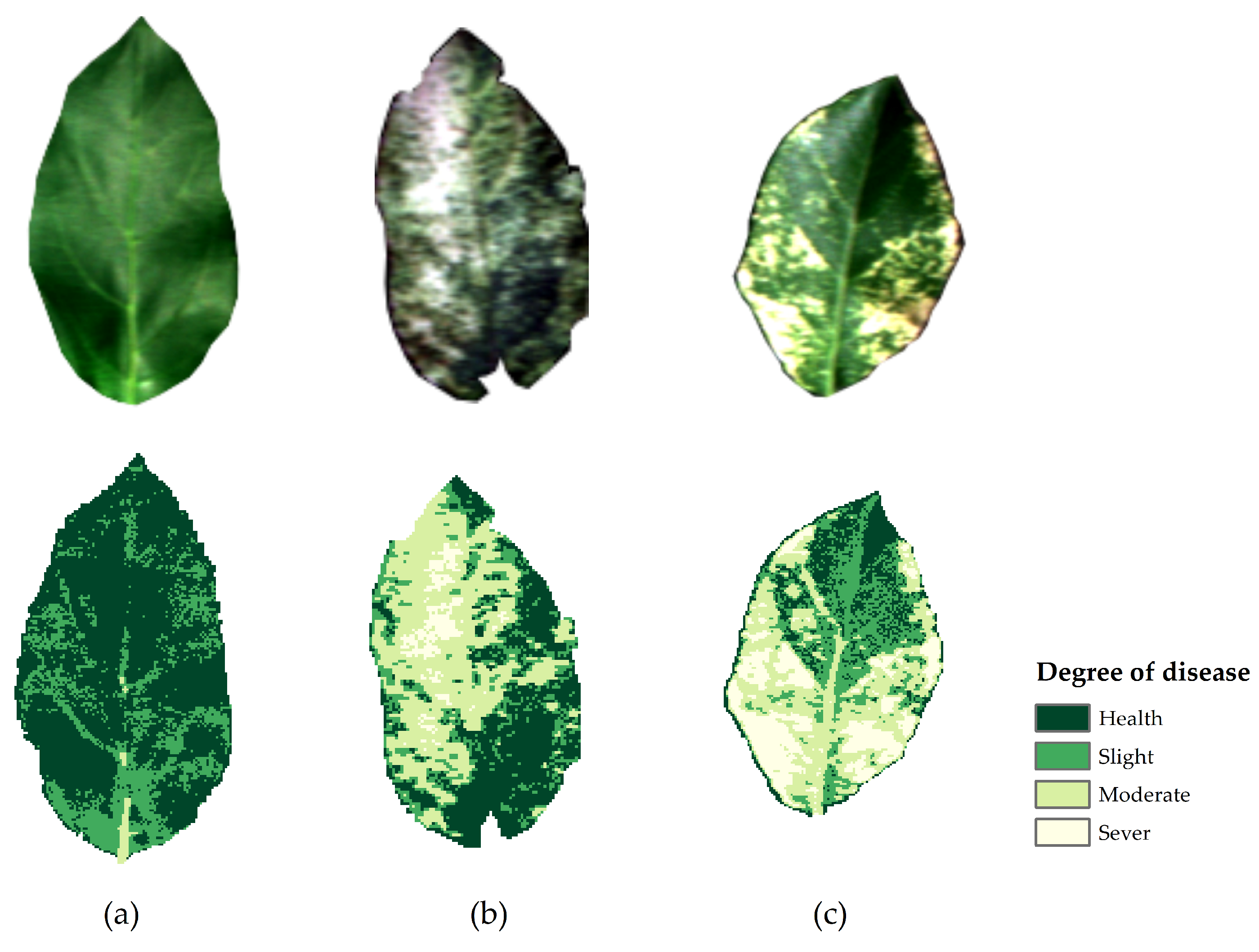
3.4. Inversion of Degree of Mosaic Disease in Hyperspectral Images

In the Envi environment, a mask tool was used to remove the background and extract the hyperspectral images of the leaves. The hyperspectral image of apple leaves was solved pixel-by-pixel using the VPs-XGBoost model to obtain the anthocyanin content distribution in apple leaves. The value of each pixel represents the anthocyanin content at a point on the leaf. Next, according to the relationship between the anthocyanin content and the degree of apple leaf mosaic disease, the degree of mosaic disease inversion mapping was performed to obtain a distribution diagram of the apple leaf mosaic disease grade. Finally, the disease degree of the entire leaf was evaluated based on the disease degree of each pixel on each leaf.

In this study, three leaves were randomly selected for inversion, and the results are shown in Figure 8. The inversion maps of the three leaf groups were highly similar to their true color images. Among them, outliers appearing in the inversion map of group (a) (at the position of the main vein, removed during the statistical period) were found to be caused by strong reflection at the leaf veins caused by excessively strong light when shooting. Leaves were judged to be mildly diseased based on the proportion of diseased pixels. For the leaves of group (b), although the affected area of the leaves was widely distributed according to the true color image, severe pixels accounted for only 5.52%, and diseased pixels accounted for 70.97% of the total; therefore, this could be judged as moderately diseased. It can be seen from

Table 8. Anthocyanin content: characteristics of the pixels.

	Min	Max	Average	Number of Pixels	Healthy Pixels %	Slight Pixels %	Moderate Pixels %	Severe Pixels %
(a)	0.429	0.550	0.490	11949	56.87	41.98	1.15	0.00
(b)	0.442	0.764	0.581	6880	29.03	25.23	40.36	5.52
(c)	0.423	0.860	0.612	10432	13.60	31.93	34.16	20.30

that the anthocyanin content in the leaves in group (c) was as high as 0.84, and the pixels that belonged to the severe infection group (content of anthocyanin >0.71) accounted for 20.30% of the total number of pixels. Therefore, based on the combination of anthocyanin content and spot proportion in the infection map, it was determined that it belonged to severely infected leaves. The results showed that it is feasible to invert the anthocyanin content based on VPs-XGBoost to determine the degree of mosaic disease in apple leaves.

4. Discussion

4.1. Spectral Reflectance of Leaves Closely Relates to Degree of Mosaic Disease

Hyperspectral remote sensing has become an automatic, objective, and rapid method for automated monitoring of photosynthetic pigments, diseases, and insect pests in crops. Previous studies have shown that the red-edge region is less sensitive to the environment and soil background [72] and can provide more accurate information for detecting the crop stress state, light, and pigment absorption [73]. To use spectral reflectance measurements effectively for disease detection, it is crucial to identify the most important spectral wavelengths that are closely associated with a particular disease. In this study, when the anthocyanin content was <0.49, the reflectance characteristics of the diseased and healthy leaves showed little difference in the visible range, and the spectral characteristics were similar. This result is consistent with that of a study by Luo L [25] that showed no significant differences in the spectra of healthy maize leaves and those mildly infected with dwarf mosaic disease. When the anthocyanin content was higher than 0.49, that is, when the disease was more serious, the spectra of the infected leaves and healthy leaves were significantly different in the visible and near-infrared regions, which is also consistent with the conclusion by Luo L. To effectively apply spectral reflectance measurements to crop disease monitoring, this study found that the wavelength closely related to mosaic infection was 518–702 nm, and the correlation coefficient was up to 0.84, according to the type and application range of the mosaic disease.

4.2. Vegetation Index and Wavelet Coefficients of any Two Bands have Higher Accuracy for Monitoring Mosaic Disease

Compared with VI_S, the traditional vegetation indices constructed using specific wavelengths and VI_A constructed with any two bands had a higher correlation with the leaf anthocyanin content, indicating that their accuracy in monitoring the degree of mosaic disease was higher. This conclusion is consistent with that of the following study: Mahlein drew a contour map of the correlation coefficient of leaf spot, rust, and powdery mildew disease severity in sugar beets based on any 2-band NDVI and used it to identify and monitor plant diseases [74]. Wang proposed that the red-edge normalized vegetation index (DVI) could be used to monitor corn big spot disease [75]. Deng proposed that NDVI, TVI, MTVI1, and MCARI2 constructed with all bands performed better in monitoring citrus yellow dragon disease [14]. The core bands in these studies were 500–750 nm, which were close to the optimal band range obtained in the present study.

The correlations between the wavelet coefficients and anthocyanin in the characteristic curves of the reflection spectra obtained by the transformation of different parent waves were slightly different; however, the sensitive bands were similar, concentrated at 480–550 nm and 760–800 nm. Compared to the characteristic bands and VI_S, the correlation between the wavelet coefficients and leaf anthocyanin content was significantly stronger. Consequently, the prediction accuracy of the anthocyanin content was improved by the decomposition of wavelet coefficients obtained from the spectral data [29,33]. Nonetheless, this result differs from the sensitive bands of 470–485 nm, 520–600 nm, and 630–760 nm proposed by Shi in a study of wheat yellow rust [28]. This difference may be because of the different responses of plants and diseases to the spectrum. In the established model, the accuracy of the λ_CWT-models improved significantly compared with the feature-band models and the single species vegetation index models, which was consistent with the conclusion obtained by Guo [58] when inverting the chlorophyll content of the six plant-coverts. Except for the λ_CWT-PLSR model, the accuracy of other λ_CWT-models was lower than that of the VI-models, which may be caused by the redundancy of wavelet information. In future, an optimal factor selection of the wavelet coefficient should be conducted to obtain a more accurate estimation model [76].

4.3. Application of Machine Learning Algorithm to Monitoring Mosaic Disease

Hyperspectral remote sensing methods for estimating plant physiological and biochemical parameters primarily include physical radiation transfer and empirical statistical models [25]. Most empirical statistical models are built based on vegetation indices, and their structures are simple and diverse. These models are sensitive to vegetation type, light conditions, canopy structure, and soil background; therefore, their versatility is poor. The advantage of the machine learning model is that it can realize the high-precision prediction of leaf pigments by analyzing the relationship between leaf nutrient drivers and pigment content without relying on specific crop parameters. In particular, the prediction and practical performance of the models in this study were improved using multiple parameters (VP_s). We conclude that the use of S–G to pretreat the spectrum and select effective variables for optimizing the model and improving the prediction accuracy is feasible. VP_s-XGBoost has strong potential for monitoring the degree of apple mosaic disease. However, this study was conducted at the apple leaf scale, which will have limitations when other datasets or crops are encountered. Therefore, the model should continue to be optimized in the future to create a model suitable for the canopy scale or different crops.

5. Conclusions

Healthy and diseased apple leaves were investigated and the reflection spectrum and anthocyanin content of different degrees of mosaic disease were observed. Differences between the healthy and diseased leaves were analyzed and the characteristics of leaves with different degrees of mosaic disease were compared. Then, the anthocyanin estimation models were constructed using the PLSR, RF, ANN, and XGBoost methods according to the selected feature bands, vegetation indices, wavelet coefficients, and multiple parameter combinations. Finally, the anthocyanin content of the apple leaves was estimated using the optimal model and the degree of mosaic disease was monitored and evaluated. Our conclusions are as follows:

• The spectral difference between the healthy and diseased leaves was concentrated in the range of 470–750 nm, with the largest difference appearing near 702 nm. With the increase in the severity of mosaic disease, the anthocyanin content increased, the absorption characteristics gradually disappeared at 500–560 nm, and the phenomenon called “blue shift” appeared at the reflection spectrum of the red edge.
• Wavelets transformed the decomposed spectral information and effectively improved the correlation between the reflectance spectrum and anthocyanin content. Moreover, the accuracy of the anthocyanin regression models constructed using wavelet coefficients was significantly improved compared to the anthocyanin regression models constructed using characteristic bands and vegetation indices.
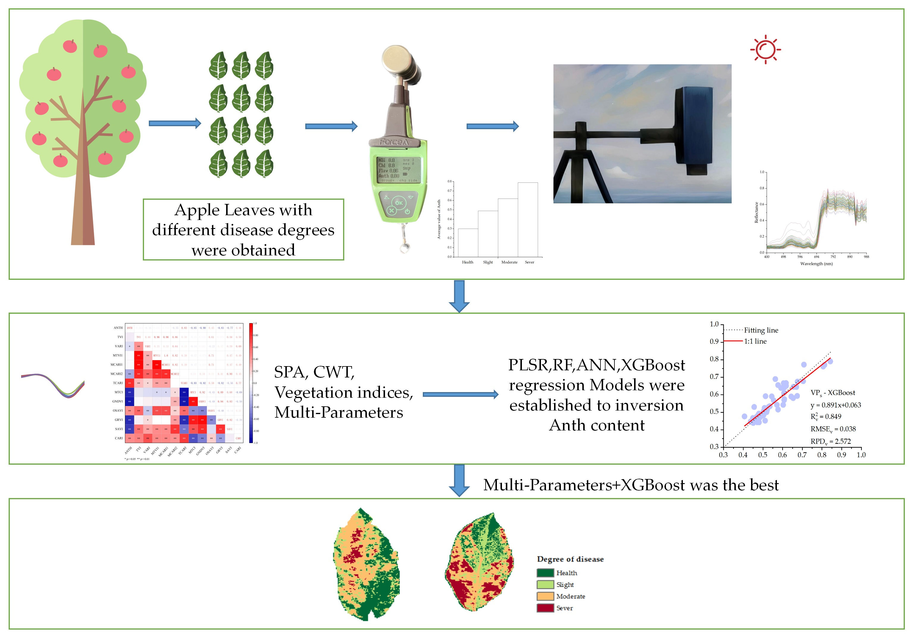
• The VPs-XGBoost estimation model based on multiple parameters (R²_v = 0.849, RPD = 2.572) was more accurate and reliable than the other methods. The VPs-XGBoost method, based on hyperspectral images, may be a rapid, accurate, and simple method to monitor the degree of mosaic disease in apple leaves.

References

1. FAOSTAT. Available online: https://www.fao.org/faostat/en/#data/QCL/visualize (accessed on 6 February 2023).
2. Hu, G.-J.; Dong, Y.-F.; Zhang, Z.-P.; Fan, X.-D.; Ren, F. Molecular characterization of Apple necrotic mosaic virus identified in crabapple (Malus spp.) tree of China. J. Integr. Agric. 2019, 18, 698–701. [Google Scholar] [CrossRef]
3. Shi, W.; Yao, R.; Sunwu, R.; Huang, K.; Liu, Z.; Li, X.; Yang, Y.; Wang, J. Incidence and Molecular Identification of Apple Necrotic Mosaic Virus (ApNMV) in Southwest China. Plants 2020, 9, 415. [Google Scholar] [CrossRef] [PubMed]
4. Noda, H.; Yamagishi, N.; Yaegashi, H.; Xing, F.; Xie, J.; Li, S.; Zhou, T.; Ito, T.; Yoshikawa, N. Apple necrotic mosaic virus, a novel ilarvirus from mosaic-diseased apple trees in Japan and China. J. Gen. Plant Pathol. 2017, 83, 83–90. [Google Scholar] [CrossRef]
5. Chalker-Scott, L. Environmental Significance of Anthocyanins in Plant Stress Responses. Photochem. Photobiol. 1999, 70, 1–9. [Google Scholar] [CrossRef]
6. Sullivan, C.N.; Koski, M.H. The effects of climate change on floral anthocyanin polymorphisms. Proc. Biol. Sci. 2021, 288, 20202693. [Google Scholar] [CrossRef]
7. Gitelson, A.A.; Merzlyak, M.N.; Chivkunova, O.B. Optical Properties and Nondestructive Estimation of Anthocyanin Content in Plant Leaves. Photochem. Photobiol. 2001, 74, 38–45. [Google Scholar] [CrossRef]
8. Gitelson, A.A. Non-Destructive Assessment of Chlorophyll Carotenoid and Anthocyanin Content in Higher Plant Leaves: Principles and Algorithms. 2004. Available online: https://digitalcommons.unl.edu/natrespapers/263/ (accessed on 23 April 2023).
9. Steele, M.R.; Gitelson, A.A.; Rundquist, D.C.; Merzlyak, M.N. Nondestructive Estimation of Anthocyanin Content in Grapevine Leaves. Am. J. Enol. Vitic. 2009, 60, 87–92. [Google Scholar] [CrossRef]
10. Qin, J.; Rundquist, D.; Gitelson, A.; Tan, Z.; Steele, M. A Non-linear Model of Nondestructive Estimation of Anthocyanin Content in Grapevine Leaves with Visible/Red-Infrared Hyperspectral. In Proceedings of the Computer and Computing Technologies in Agriculture IV, Nanchang, China, 22–25 October 2010; Volume 3, pp. 47–62. [Google Scholar]
11. Jiang, J.; Zhang, Z.; Cao, Q.; Liang, Y.; Krienke, B.; Tian, Y.; Zhu, Y.; Cao, W.; Liu, X. Use of an Active Canopy Sensor Mounted on an Unmanned Aerial Vehicle to Monitor the Growth and Nitrogen Status of Winter Wheat. Remote Sens. 2020, 12, 3684. [Google Scholar] [CrossRef]
12. Terentev, A.; Dolzhenko, V.; Fedotov, A.; Eremenko, D. Current State of Hyperspectral Remote Sensing for Early Plant Disease Detection: A Review. Sensors 2022, 22, 757. [Google Scholar] [CrossRef]
13. Wang, J.; Ren, G.; Lin, Z.; Wang, A.; Hu, Y.; Li, X.; Wu, P.; Ma, Y.; Zhang, J. Estimation of Aboveground Vegetation Nitrogen Contents in the Yellow River Estuary Wetland Using GaoFen-1 Remote Sensing Data. J. Coastal Res. 2020, 102, 1–10. [Google Scholar] [CrossRef]
14. Deng, X.; Huang, Z.; Zheng, Z.; Lan, Y.; Dai, F. Field detection and classification of citrus Huanglongbing based on hyperspectral reflectance. Comput. Electron. Agric. 2019, 167, 105006. [Google Scholar] [CrossRef]
15. Haboudane, D. Hyperspectral vegetation indices and novel algorithms for predicting green LAI of crop canopies: Modeling and validation in the context of precision agriculture. Remote Sens. Environ. 2004, 90, 337–352. [Google Scholar] [CrossRef]
16. Haboudane, D.; Miller, J.R.; Tremblay, N.; Zarco-Tejada, P.J.; Dextraze, L. Integrated narrow-band vegetation indices for prediction of crop chlorophyll content for application to precision agriculture. Remote Sens. Environ. 2002, 81, 416–426. [Google Scholar] [CrossRef]
17. Pal, T.; Jaiswal, V.; Chauhan, R.S. DRPPP: A machine learning based tool for prediction of disease resistance proteins in plants. Comput. Biol. Med. 2016, 78, 42–48. [Google Scholar] [CrossRef] [PubMed]
18. Shafri, H.Z.M.; Hamdan, N. Hyperspectral Imagery for Mapping Disease Infection in Oil Palm Plantation Using Vegetation Indices and Red Edge Techniques. Am. J. Appl. Sci. 2009, 6, 1031–1035. [Google Scholar]
19. Sun, Q.; Jiao, Q.; Qian, X.; Liu, L.; Liu, X.; Dai, H. Improving the Retrieval of Crop Canopy Chlorophyll Content Using Vegetation Index Combinations. Remote Sens. 2021, 13, 470. [Google Scholar] [CrossRef]
20. Liu, X.; Ji, L.; Zhang, C.; Liu, Y. A method for reconstructing NDVI time-series based on envelope detection and the Savitzky-Golay filter. Int. J. Digit. Earth 2022, 15, 553–584. [Google Scholar] [CrossRef]
21. Ruffin, C.; King, R.L.; Younan, N.H. A Combined Derivative Spectroscopy and Savitzky-Golay Filtering Method for the Analysis of Hyperspectral Data. GISci. Remote Sens. 2013, 45, 1–15. [Google Scholar] [CrossRef]
22. Wang, J.; Shi, T.; Liu, H.; Wu, G. Successive projections algorithm-based three-band vegetation index for foliar phosphorus estimation. Ecol. Indic. 2016, 67, 12–20. [Google Scholar] [CrossRef]
23. Ding, D.; Yu, H.; Yin, Y.; Yuan, Y.; Li, Z.; Li, F. Determination of Chlorophyll and Hardness in Cucumbers by Raman Spectroscopy with Successive Projections Algorithm (SPA)—Extreme Learning Machine (ELM). Anal. Lett. 2022, 56, 1216–1228. [Google Scholar] [CrossRef]
24. Gitelson, A.A.; Keydan, G.P.; Merzlyak, M.N. Three-band model for noninvasive estimation of chlorophyll, carotenoids, and anthocyanin contents in higher plant leaves. Geophys. Res. Lett. 2006, 33, L11402. [Google Scholar] [CrossRef]
25. Luo, L.; Chang, Q.; Wang, Q.; Huang, Y. Identification and Severity Monitoring of Maize Dwarf Mosaic Virus Infection Based on Hyperspectral Measurements. Remote Sens. 2021, 13, 4560. [Google Scholar] [CrossRef]
26. Ma, H.; Huang, W.; Jing, Y.; Pignatti, S.; Laneve, G.; Dong, Y.; Ye, H.; Liu, L.; Guo, A.; Jiang, J. Identification of Fusarium Head Blight in Winter Wheat Ears Using Continuous Wavelet Analysis. Sensors 2019, 20, 20. [Google Scholar] [CrossRef] [PubMed]
27. Zhang, J.; Sun, H.; Gao, D.; Qiao, L.; Liu, N.; Li, M.; Zhang, Y. Detection of Canopy Chlorophyll Content of Corn Based on Continuous Wavelet Transform Analysis. Remote Sens. 2020, 12, 2741. [Google Scholar] [CrossRef]
28. Shi, Y.; Huang, W.; González-Moreno, P.; Luke, B.; Dong, Y.; Zheng, Q.; Ma, H.; Liu, L. Wavelet-Based Rust Spectral Feature Set (WRSFs): A Novel Spectral Feature Set Based on Continuous Wavelet Transformation for Tracking Progressive Host–Pathogen Interaction of Yellow Rust on Wheat. Remote Sens. 2018, 10, 525. [Google Scholar] [CrossRef]
29. Wang, Z.; Chen, J.; Fan, Y.; Cheng, Y.; Wu, X.; Zhang, J.; Wang, B.; Wang, X.; Yong, T.; Liu, W.; et al. Evaluating photosynthetic pigment contents of maize using UVE-PLS based on continuous wavelet transform. Comput. Electron. Agric. 2020, 169, 105160. [Google Scholar] [CrossRef]
30. Ferwerda, J.G.; Jones, S.D. Continuous Wavelet Transformations for Hyperspectral Feature Detection. In Progress in Spatial Data Handling: 12th International Symposium on Spatial Data Handling; Riedl, A., Kainz, W., Elmes, G.A., Eds.; Springer: Berlin, Heidelberg, 2006; pp. 167–178. [Google Scholar]
31. Zhao, L.; Li, Q.; Zhang, Y.; Wang, H.; Du, X. Integrating the Continuous Wavelet Transform and a Convolutional Neural Network to Identify Vineyard Using Time Series Satellite Images. Remote Sens. 2019, 11, 2641. [Google Scholar] [CrossRef]
32. He, R.; Li, H.; Qiao, X.; Jiang, J. Using wavelet analysis of hyperspectral remote-sensing data to estimate canopy chlorophyll content of winter wheat under stripe rust stress. Int. J. Remote Sens. 2018, 39, 4059–4076. [Google Scholar] [CrossRef]
33. An, G.; Xing, M.; Liao, C.; He, B. Estimating Chlorophyll Content of Rice Based on UAV-Based Hyperspectral Imagery and Continuous Wavelet Transform. In Proceedings of the IGARSS 2020—2020 IEEE International Geoscience and Remote Sensing Symposium, Waikoloa, Hawaii, 26 September–2 October 2020; pp. 5270–5273. [Google Scholar]
34. Bagheri, N.; Mohamadi-Monavar, H.; Azizi, A.; Ghasemi, A. Detection of Fire Blight disease in pear trees by hyperspectral data. Eur. J. Remote Sens. 2017, 51, 1–10. [Google Scholar] [CrossRef]
35. Gold, K.M.; Townsend, P.A.; Chlus, A.; Herrmann, I.; Couture, J.J.; Larson, E.R.; Gevens, A.J. Hyperspectral Measurements Enable Pre-Symptomatic Detection and Differentiation of Contrasting Physiological Effects of Late Blight and Early Blight in Potato. Remote Sens. 2020, 12, 286. [Google Scholar] [CrossRef]
36. Huang, W.; Lamb, D.W.; Niu, Z.; Zhang, Y.; Liu, L.; Wang, J. Identification of yellow rust in wheat using in-situ spectral reflectance measurements and airborne hyperspectral imaging. Precis. Agric. 2007, 8, 187–197. [Google Scholar] [CrossRef]
37. Xie, C.; He, Y. Spectrum and Image Texture Features Analysis for Early Blight Disease Detection on Eggplant Leaves. Sensors 2016, 16, 676. [Google Scholar] [CrossRef] [PubMed]
38. Nagasubramanian, K.; Jones, S.; Singh, A.K.; Sarkar, S.; Singh, A.; Ganapathysubramanian, B. Plant disease identification using explainable 3D deep learning on hyperspectral images. Plant Methods 2019, 15, 98. [Google Scholar] [CrossRef] [PubMed]
39. Polder, G.; Blok, P.M.; de Villiers, H.A.C.; van der Wolf, J.M.; Kamp, J. Potato Virus Y Detection in Seed Potatoes Using Deep Learning on Hyperspectral Images. Front. Plant Sci. 2019, 10, 209. [Google Scholar] [CrossRef]
40. Yuan, L.; Yan, P.; Han, W.; Huang, Y.; Wang, B.; Zhang, J.; Zhang, H.; Bao, Z. Detection of anthracnose in tea plants based on hyperspectral imaging. Comput. Electron. Agric. 2019, 167, 105039. [Google Scholar] [CrossRef]
41. Wu, Y.; Cao, Y.; Zhai, Z. Early Detection of Bacterial Blight in Hyperspectral Images Based on Random Forest and Adaptive Coherence Estimator. Sustainability 2022, 14, 13168. [Google Scholar] [CrossRef]
42. Xu, S.; Xu, X.; Blacker, C.; Gaulton, R.; Zhu, Q.; Yang, M.; Yang, G.; Zhang, J.; Yang, Y.; Yang, M.; et al. Estimation of Leaf Nitrogen Content in Rice Using Vegetation Indices and Feature Variable Optimization with Information Fusion of Multiple-Sensor Images from UAV. Remote Sens. 2023, 15, 854. [Google Scholar] [CrossRef]
43. Tao, H.; Feng, H.; Xu, L.; Miao, M.; Yang, G.; Yang, X.; Fan, L. Estimation of the Yield and Plant Height of Winter Wheat Using UAV-Based Hyperspectral Images. Sensors 2020, 20, 1231. [Google Scholar] [CrossRef]
44. Ta, N.; Chang, Q.; Zhang, Y. Estimation of Apple Tree Leaf Chlorophyll Content Based on Machine Learning Methods. Remote Sens. 2021, 13, 3902. [Google Scholar] [CrossRef]
45. Wei, M.; Wang, H.; Zhang, Y.; Li, Q.; Du, X.; Shi, G.; Ren, Y. Investigating the Potential of Crop Discrimination in Early Growing Stage of Change Analysis in Remote Sensing Crop Profiles. Remote Sens. 2023, 15, 853. [Google Scholar] [CrossRef]
46. Couture, J.J.; Singh, A.; Charkowski, A.O.; Groves, R.L.; Gray, S.M.; Bethke, P.C.; Townsend, P.A. Integrating Spectroscopy with Potato Disease Management. Plant Dis. 2018, 102, 2233–2240. [Google Scholar] [CrossRef] [PubMed]
47. Li, F.; Wang, L.; Liu, J.; Wang, Y.; Chang, Q. Evaluation of Leaf N Concentration in Winter Wheat Based on Discrete Wavelet Transform Analysis. Remote Sens. 2019, 11, 1331. [Google Scholar] [CrossRef]
48. Qi, H.; Zhu, B.; Kong, L.; Yang, W.; Zou, J.; Lan, Y.; Zhang, L. Hyperspectral Inversion Model of Chlorophyll Content in Peanut Leaves. Appl. Sci. 2020, 10, 2259. [Google Scholar] [CrossRef]
49. Lussem, U.; Bolten, A.; Gnyp, M.L.; Jasper, J.; Bareth, G. Evaluation of Rgb-Based Vegetation Indices from Uav Imagery To Estimate Forage Yield in Grassland. In Proceedings of the International Archives of the Photogrammetry, Remote Sensing and Spatial Information Sciences, Beijing, China, 7–10 May 2018; pp. 1215–1219. [Google Scholar]
50. Sharifi, A. Remotely sensed vegetation indices for crop nutrition mapping. J. Sci. Food. Agric. 2020, 100, 5191–5196. [Google Scholar] [CrossRef] [PubMed]
51. Rondeaux, G.; Steven, M.; Baret, F. Optimization of soil-adjusted vegetation indices. Remote Sens. Environ. 1996, 55, 95–107. [Google Scholar] [CrossRef]
52. Nagai, S.; Ishii, R.; Suhaili, A.B.; Kobayashi, H.; Matsuoka, M.; Ichie, T.; Motohka, T.; Kendawang, J.J.; Suzuki, R. Usability of noise-free daily satellite-observed green–red vegetation index values for monitoring ecosystem changes in Borneo. Int. J. Remote Sens. 2014, 35, 7910–7926. [Google Scholar] [CrossRef]
53. Chen, F.; Chen, C.; Li, W.; Xiao, M.; Yang, B.; Yan, Z.; Gao, R.; Zhang, S.; Han, H.; Chen, C.; et al. Rapid detection of seven indexes in sheep serum based on Raman spectroscopy combined with DOSC-SPA-PLSR-DS model. Spectrochim. Acta Part A Mol. Biomol. Spectrosc. 2021, 248, 119260. [Google Scholar] [CrossRef]
54. The Successive Projections Algorithm (SPA) Homepage. Available online: http://www.ele.ita.br/~kawakami/spa/ (accessed on 23 April 2023).
55. Kim, M.S.; Daughtry, C.S.T.; Chappelle, E.W.; McMurtrey, J.E. The use of high spectral resolution bands for estimating absorbed photosynthetically active radiation (APAR). In Proceedings of the ISPRS’94, Val d’Isere, France, 17–21 January 1994. [Google Scholar]
56. Rivard, B.; Feng, J.; Gallie, A.; Sanchez-Azofeifa, A. Continuous wavelets for the improved use of spectral libraries and hyperspectral data. Remote Sens. Environ. 2008, 112, 2850–2862. [Google Scholar] [CrossRef]
57. Blackburn, G.; Ferwerda, J. Retrieval of chlorophyll concentration from leaf reflectance spectra using wavelet analysis. Remote Sens. Environ. 2008, 112, 1614–1632. [Google Scholar] [CrossRef]
58. Guo, Y.; Zhang, L.; Wang, D.; Ma, M. Application of Wavelete Analysis for Determining Chlorophyll Concentration in Vegetation by Hyperspectral Reflectance. Bull. Surv. Mapp. 2010, 8, 31–33,53. [Google Scholar]
59. Li, X.; Li, Z.; Chen, G.; Qiu, H.; Hou, G.; Fan, P. Prediction of Tidal Flat Sediment Moisture Content Based on Wavelet Transform. Spectrosc. Spect. Anal. 2022, 42, 1156–1161. [Google Scholar]
60. Cheng, T.; Rivard, B.; Sánchez-Azofeifa, G.A.; Feng, J.; Calvo-Polanco, M. Continuous wavelet analysis for the detection of green attack damage due to mountain pine beetle infestation. Remote Sens. Environ. 2010, 114, 899–910. [Google Scholar] [CrossRef]
61. Zhu Wen, Y.; Zhou, J.; Wu, Y.f.; Wang, M.J. Iris Feature Extraction based on Haar Wavelet Transform. Int. J. Secur. Its Appl. 2014, 8, 265–272. [Google Scholar] [CrossRef]
62. Koger, C. Wavelet analysis of hyperspectral reflectance data for detecting pitted morningglory (Ipomoea lacunosa) in soybean (Glycine max). Remote Sens. Environ. 2003, 86, 108–119. [Google Scholar] [CrossRef]
63. Cheng, J.-H.; Sun, D.-W. Partial Least Squares Regression (PLSR) Applied to NIR and HSI Spectral Data Modeling to Predict Chemical Properties of Fish Muscle. Food Eng. Rev. 2016, 9, 36–49. [Google Scholar] [CrossRef]
64. Lin, L.; Liu, X. Soil-moisture-index spectrum reconstruction improves partial least squares regression of spectral analysis of soil organic carbon. Precis. Agric. 2022, 23, 1707–1719. [Google Scholar] [CrossRef]
65. Breiman, L. Random Forests. Mach. Learn. 2001, 45, 5–32. [Google Scholar] [CrossRef]
66. Soltanikazemi, M.; Minaei, S.; Shafizadeh-Moghadam, H.; Mahdavian, A. Field-scale estimation of sugarcane leaf nitrogen content using vegetation indices and spectral bands of Sentinel-2: Application of random forest and support vector regression. Comput. Electron. Agric. 2022, 200, 107130. [Google Scholar] [CrossRef]
67. Estrada Zúñiga, A.C.; Cárdenas, J.; Víctor Bejar, J.; Ñaupari, J. Biomass estimation of a high Andean plant community with multispectral images acquired using UAV remote sensing and Multiple Linear Regression, Support Vector Machine and Random Forests models. Sci. Agropecu. 2022, 13, 301–310. [Google Scholar] [CrossRef]
68. Feng, H.; Tao, H.; Fan, Y.; Liu, Y.; Li, Z.; Yang, G.; Zhao, C. Comparison of Winter Wheat Yield Estimation Based on Near-Surface Hyperspectral and UAV Hyperspectral Remote Sensing Data. Remote Sens. 2022, 14, 4158. [Google Scholar] [CrossRef]
69. Yuan, H.; Yang, G.; Li, C.; Wang, Y.; Liu, J.; Yu, H.; Feng, H.; Xu, B.; Zhao, X.; Yang, X. Retrieving Soybean Leaf Area Index from Unmanned Aerial Vehicle Hyperspectral Remote Sensing: Analysis of RF, ANN, and SVM Regression Models. Remote Sens. 2017, 9, 309. [Google Scholar] [CrossRef]
70. Chen, T.; Guestrin, C. XGBoost. In Proceedings of the 22nd ACM SIGKDD International Conference on Knowledge Discovery and Data Mining, San Francisco, CA, USA, 13–17 August 2016; pp. 785–794. [Google Scholar]
71. Zhang, N.; Zhang, X.; Wang, C.; Li, L.; Bai, T. Cotton LAI Estimation Based on Hyperspectral and Successive Projection Algorithm. Trans. Chin. Soc. Agric. Mach. 2022, 53, 257–262. [Google Scholar]
72. Mutanga, O.; Skidmore, A.K. Red edge shift and biochemical content in grass canopies. ISPRS-J. Photogramm. Remote Sens. 2007, 62, 34–42. [Google Scholar] [CrossRef]
73. Li, L.; Ren, T.; Ma, Y.; Wei, Q.; Wang, S.; Li, X.; Cong, R.; Liu, S.; Lu, J. Evaluating chlorophyll density in winter oilseed rape (Brassica napus L.) using canopy hyperspectral red-edge parameters. Comput. Electron. Agric. 2016, 126, 21–31. [Google Scholar] [CrossRef]
74. Mahlein, A.K.; Rumpf, T.; Welke, P.; Dehne, H.W.; Plümer, L.; Steiner, U.; Oerke, E.C. Development of spectral indices for detecting and identifying plant diseases. Remote Sens. Environ. 2013, 128, 21–30. [Google Scholar] [CrossRef]
75. Wang, L.; Liu, J.; Shao, J.; Yang, F.; Gao, J. Remote sensing index selection of leaf blight disease in spring maize based on hyperspectral data. Trans. CSAE 2017, 33, 170–177. [Google Scholar]
76. Ménard, R.; Deshaies-Jacques, M. Evaluation of Analysis by Cross-Validation. Part I: Using Verification Metrics. Atmosphere 2018, 9, 86. [Google Scholar] [CrossRef]
Figure 1. Location of the experimental area and pictures of the experiments.
Remotesensing 15 02504 g001
Figure 2. Spectral characteristics of the leaves with different degrees of disease.
Remotesensing 15 02504 g002
Figure 3. Correlation between the anthocyanin content and original spectrum.
Remotesensing 15 02504 g003
Figure 4. (a) Characteristic bands selected by SPA; (b) RMSE of SPA.
Remotesensing 15 02504 g004
Figure 5. Contour maps of |r| between the vegetation indices and anthocyanin content. (ac) represent the R2 between the DSI, NDSI, and RSI, respectively, and the anthocyanin content.
Remotesensing 15 02504 g005
Figure 6. Contour map of |r| between the Gsau1 wavelet coefficient and anthocyanin content.
Remotesensing 15 02504 g006
Figure 7. Scatter diagrams of the models for estimating the anthocyanin content in apple leaves based on VPS.
Remotesensing 15 02504 g007
Figure 8. Leaf tricolor images and hyperspectral inversion map. (ac) represent mildly, moderately, severely infected apple leaves, respectively.
Remotesensing 15 02504 g008