Abstract
Information on vegetation cover and soil management is used in hydrological and soil erosion modeling, but in most cases, reference values are used solely based on land use classification without considering the actual spatial and temporal variation adopted at the field scale. This work focused on the adoption of satellite optical data from the Copernicus Sentinel-2 (S2) mission to evaluate both spatial and temporal variations of vineyard ground cover. First, on a wider scale, fields were mapped by photointerpretation, and a cluster analysis was carried out. Results suggest that vineyards can be classified according to different inter-row soil management, with the best results obtained using NDVI and NDWI. A pilot area in the municipality of Carpeneto, in the wine-growing area of Alto Monferrato, was also analyzed due to the availability of reference data on inter-row vegetation cover from experimental plots. Those are set on sloping areas and present different inter-row soil managements (conventional tillage—CT, and permanent grass cover—GC). Time series of different vegetation indices (VIs) have been obtained, and both S2 native bands and the derived VIs were evaluated to assess their capability of describing the vineyard’s inter-row coverage growth trends at plot level for the agrarian year 2017–2018. Results suggest that a seasonality effect may be involved in the choice of the most suitable band or index that better describes soil coverage development at a given moment of the year. Further studies on open-source remotely sensed (RS) data could provide specific inputs for applications in erosion risk management and crop modeling.
1. Introduction
The International Organization of Vine and Wine (OIV) aims to define the principles for sustainability in viticulture by promoting production systems and practices that can preserve and improve the conditions and use of natural resources, as well as enhancing socio-economic conditions for the operators involved in the production process [1]. Soil degradation, and soil erosion more specifically, is one of the major threats affecting agricultural soils worldwide, as stated by the Soil Thematic Strategy from the European Union [2,3] and the FAO’s Status of the World Soil Resources [4]. The EU Soil Strategy for 2030 [5] has been introduced to have, by 2050, all EU ecosystems in healthy conditions by restoring and protecting degraded soils. Vineyard agroecosystems play an important role in terms of socio-economic impacts due to interactions with the environmental and cultural aspects related to the territory of production [6]. Studies suggest that intensive agricultural practices contribute to the loss of habitats and biodiversity, increasing soil erosion and nutrient runoff [7,8], while natural vegetation has positive impacts on ecosystem services (ES) and can help decrease runoff, sediment, and nutrient losses [9,10,11,12,13,14,15].
In Italy, viticulture for wine production plays a key role in terms of planted areas, harvested volumes, and the resultant economic returns. In 2019, Italy was the first European producer (7.9 mln Mg) and the second world producer after China (14.3 mln Mg) [16]. The crop kept stable over the past years, with more than 630,000 hectares cultivated [17]. Piedmont (NW Italy) is an Italian region with a tradition of high-quality wine-making, with more than 40,000 hectares of vineyards, mostly on hilly areas (more than 88% of the cultivated surface). Those often present erosion rates higher than 15 Mg ha−1 year−1 [18]. Some areas are also important in terms of landscape value: the territory of Langhe-Roero and Monferrato, for instance, is listed on the UNESCO World Heritage List (whc.unesco.org (accessed on 20 October 2022)).
Management decisions in tree crops such as orchards and vineyards are usually influenced by water availability and pedoclimatic conditions of the area, and the perception of benefits and drawbacks related to the adoption of ES such as inter-row cover crops or natural grass cover can be highly variable. Sustainability can be achieved by adopting practices and technologies that allow farmers to operate site-specifically, addressing the inputs required to ensure high yields [19]. Sensors are typically used in precision farming to analyze crop and soil response, allowing the execution of specific operations. In the wine-making sector, precision viticulture has much potential, such as the adoption of field sensors for monitoring crops and production [20] and the use of machines equipped with GNSS systems for localized variable-rate applications [21,22,23].
Sensors at higher distances also play a relevant role in crop monitoring. Satellites for Earth observation (EO) are able to acquire multispectral images with a regular temporal frequency, encoding the variations of the spectral behavior of a surface. This allows describing its spatial and temporal variations. The use of remotely sensed data to support decision-making processes has recently increased in the agricultural and forestry sectors [24,25,26,27,28]. With regard to viticulture, airborne and satellite imagery can be used to describe the spatial variability of crop yield and characterize soil properties and crop variety or diseases [29,30,31,32,33,34].
VIs can be used to obtain information about phenology, water content, and biomass development throughout the growing season (GS) with a multi-temporal approach. Over the last decades, many VIs have been developed [35,36,37,38,39]; among them, the Normalized Difference Vegetation Index (NDVI) is the most used to describe crop growth dynamics. The potential of such data for viticulture is based on the relationship between canopy properties and the qualitative-quantitative yield of bunches [40,41,42,43]. Crop vigor is an expression of its spatial variability based on environmental conditions and can be quantified by measuring the crop density within the field. For tree crops, in general, vigor is expressed both in terms of plant density as well as canopy size. Based on the higher or lower spatial resolution of the available RS data, plant vigor and phenology can be investigated either at the plant or field level [25,32,44,45,46]. On the other hand, inter-row management is also very important, and the understanding of growth dynamics is fundamental for purposes, such as proper modeling of water dynamics [47,48,49,50,51,52] and soil erosion risk assessment [53,54,55,56,57,58,59], to address farmers’ choices over the most suitable inter-row soil management.
Some satellites allow the acquisition of information with a high spatial resolution (<10 m), but such data are usually provided by private companies as a paid service and require significant knowledge of data processing. Nevertheless, the resolution of such data does not always allow discrimination between the elements of the orchard/vineyard (i.e., row crop and inter-row) since vine canopy represents a small portion of the field area. Additionally, open-source satellites, such as the S2 mission, can provide images of up to 10 m of spatial resolution and at a high temporal frequency. Such resolution does not allow discriminating between the different components of the field; nevertheless, in the present study, open-source data from the S2 mission are exploited considering a multi-temporal approach, which allows, besides their spatial resolution, an analysis at the field scale. Temporal series of different VIs and spectral bands are analyzed in this work to define the vineyard’s features (in particular, those regarding the inter-row). At a local scale, the analysis based on the temporal variations of different VIs is used to assess spatial (inter-field) variations of vineyard soil management, namely to recognize whether a vineyard is managed with bare soil or ground cover in the inter-row. Then, given different inter-row management at the plot scale, the spectral information is used to assess the intensity of ground cover.
The objective of this study is to propose a methodology that allows: (i) to identify different inter-row soil managements in vineyards from open-source RS data and (ii) to describe the growth dynamics of cover crops within the inter-row when the adopted soil management is known. Furthermore, a weighted version of the well-known NDVI was also tested and compared with field measurements for ground cover, in order to evaluate its response in assessing the inter-row vegetative growth. An initial analysis was performed to assess the capability of different VIs to identify different vineyard inter-row soil management (grass-covered vs. bare soil) by using open-source remotely sensed data. Afterward, since field measurements from previous studies about ground cover were available at the plot scale [60], the relationship between estimated ground cover and the signal of spectral bands and VIs was evaluated.
2. Materials and Methods
2.1. Study Area
This work relies on data from experimental plots located in the administrative province of Alessandria (AL, Piedmont). We focused on its hilly areas, where viticulture represents the most widespread crop. Two zones have been taken into consideration for the first part of this study: (i) a calibration area set in the municipality of Carpeneto in Alto Monferrato, and (ii) a validation area, corresponding to the municipality of Gavi (Figure 1). According to the Köppen–Geiger classification [61,62], the area is characterized by a Csa (hot-summer Mediterranean) climate, with cold wet winters and hot dry summers, and the temperature of the warmest month can be equal or higher than 22 °C. Over all of the municipalities, the most recurring soils are: (i) Typic and Vertic Haplustalf, and Typic Ustorthent in Carpeneto, and (ii) Typic Haplustalf, and Typic Ustorthent in Gavi [63].
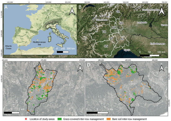
Figure 1.
Localization of the study sites (A) from a wider point of view and (B) at the regional scale. The municipalities of (C) Carpeneto and (D) Gavi are the calibration and validation site, respectively. Vineyards in both areas are distinguished according to inter-row soil management.
The experimental plots are located in the municipality of Carpeneto (AL), within the Experimental Vine and Wine Centre Tenuta Cannona (44°40N, 8°37E, 296 m above sea level) of Agrion Foundation. The vineyards of Tenuta Cannona lie on Pleistocenic fluvial terraces in the Tertiary Piedmont Basin and are characterized by highly altered gravel, sand, and silty-clay deposits, with red alteration products [64]. Soil texture in the area ranges from clay to clay-loam and is classified as Typic Ustorthents, fine-loamy, mixed, calcareous, mesic [63] or Dystric Cambisols [65]. The study site is equipped with a weather station, providing daily and hourly data for temperature and rainfall. The average annual precipitation recorded (reference period 2000–2016) in the area was 852 mm, with rainfall concentrated mainly in autumn (October and November) and spring (March), while July was the driest month. The average annual air temperature observed was 13 °C [66]. As indicated in the annual ARPA Regional reports, 2017 and 2018 have been exceptionally warm years, with an average thermal anomaly of +1.5 °C compared to the historical reference series (1971–2000). Regarding the pluviometric regime, while 2017 was an extremely dry year, 2018 was remarkably rainy (+32% compared to the reference series). In addition to the positive rainfall anomaly due to the prolonged bad weather that took place from 27 October to 7 November 2018, the province of Alessandria was also affected by an important rainy event in mid-July (Figure 2).
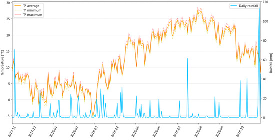
Figure 2.
Climatic trend (temperature and precipitation) during the agrarian year 2017–2018. Data were collected by the weather station nearby the experimental plots at the Tenuta Cannona. Abnormal rainy events reported at the end of October also continued during the first half of November 2018.
The Cannona experimental plots (Figure 3) are part of a larger vineyard planted in 1988 with Vitis vinifera L. cv. Barbera. The plants are located on a hillslope with an average slope of 15% and SE aspect. Each plot is 74 m long and 16.5 m wide, with an area of 1221 m2. The inter-row spacing is 2.4 m, while vine plants are spaced 1.0 m along the row and managed according to conventional viticulture practices. Each experimental plot consists of 7 vine rows set with an up-and-down orientation. Since 2000, plots have displayed different types of soil management: (i) conventional tillage (CT), using a chisel plow in the second half of April and after harvest, at a depth of about 0.25 m, while (ii) the second plot was treated with permanent grass cover (GC), controlled throughout multiple mowings during the growing season. Apart from the initial tillage operation in spring, mulching in the inter-rows and other operations, such as vines’ topping, were carried out in the same periods on both plots (Table 1). Knowing when mowings are performed can help to correctly assess the effect of mechanical operations on vegetation growth and soil surface coverage.
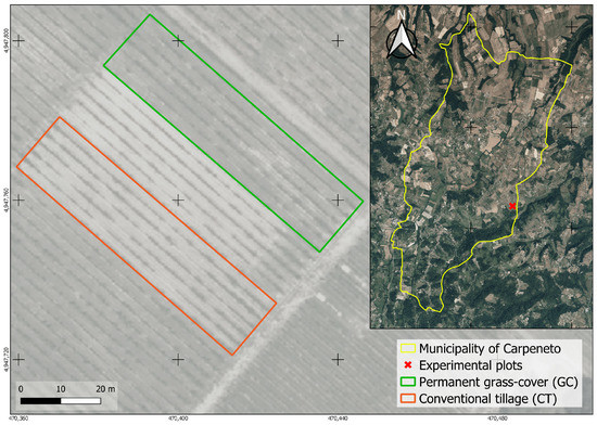
Figure 3.
Localization of the plots within the Experimental Vine and Wine Centre of Agrion Foundation, in Tenuta Cannona, in the municipality of Carpeneto (AL).

Table 1.
Mechanical interventions carried out in the experimental plots.
2.2. Available Satellite Data
2.2.1. Data Collecting and Pre-Processing
The remotely sensed data used for this work came from the ESA’s Sentinel-2 mission, consisting of two twin satellites (S2A and S2B) that ensure a high-frequency of data acquisition every 5 days, with a radiometric resolution of 12 bits. The Multi-Spectral Instrument (MSI) sensor mounted on both satellites is a filter-based push-broom imager, measuring 13 spectral bands from visible and Near Infrared (NIR) to Short-Wave Infrared (SWIR). The images acquired have a spatial resolution ranging from 10 to 60 m [67,68]. Coastal aerosol (band 1), water vapor (band 9), and cirrus (band 10), having a coarser geometric resolution (60 m) and being designed to assess atmospherical features, were not considered. For this study, all the bands considered (Table 2) whose ground sampling distance (GSD) resolution was higher than 10 m have been rescaled for homogeneity in further elaborations.
Table 2.
Technical features of S2 MSI spectral bands considered in this study.
Sentinel-2 level-2A data provide surface reflectance values (also called bottom-of-atmosphere) for different spectral bands that have been processed throughout scene classification and atmospheric and topographic correction [69,70]. Images were obtained for free via the Google Earth Engine (GEE), a cloud computing platform accessible via an internet-based application programming interface (API) and an associated web-based interactive development environment (IDE) that enables rapid prototyping and visualization of results [71,72]. Only the images whose cloud cover was lower than 20% in the corresponding S2 tile were considered for the agrarian year 2017–2018 (starting 1 November 2017, ending 31 October 2018), generating a raw time series (TS) for every S2 native band that we chose to investigate. To obtain a dataset with regular time intervals, interpolation was applied at a pixel level to generate a 10-day-stepped TS [73]. This procedure was performed on the TS of every considered spectral band, and data were successively smoothed by applying a Savitzky–Golay filter [74].
2.2.2. Vegetation Indices
Optical remote sensing can be used for qualitative and quantitative evaluations of vegetation and land cover, plant vigor, and phenology, by analyzing the electromagnetic wave reflectance in different spectral regions through passive sensors [75,76]. VIs are the result of the combination of two or more spectral bands. They are designed to enhance the contribution of vegetation properties and allow reliable spatial and temporal inter-comparisons of terrestrial photosynthetic activity and canopy structural variations [77,78].
Starting from the available surface reflectance values for the reference period, different vegetation indices have been obtained (Table 3) from the combination of TS of the S2 native bands. Maps for every index have been obtained by raster calculation from the calibrated bands of the original S2 images. In particular, we chose to use the normalized difference vegetation index (NDVI) [35], which is one of the most widely used spectral indices. Its popularity is due to its robustness and versatility for applications in different environmental and agricultural contexts [26,79,80,81,82,83,84]. Similar to NDVI, we also tested the response of the Normalized Difference Water Index (NDWI) [38], where instead of the red reflectance, the band in the SWIR is used, allowing the detection of variations in vegetation water content, making the NDWI a suitable proxy for detecting water stress. Another interesting index that has been taken into consideration is the Normalized Difference Red-Edge index (NDRE) [85], which appears less sensitive to atmospheric effects compared to NDVI. Information provided by the red-edge band is particularly useful in describing plant health. In fact, NDRE is able to detect the chlorophyll content of vegetation canopies and can be a good proxy to assess plant nitrogen content [86]. Normalized indices such as NDVI and NDWI are widely used since they have been proven reliable in describing growth dynamics for a wide variety of crops. However, NDVI appears to be sensitive to the effects of soil brightness, soil color, atmosphere, clouds, and canopy shadow and may require a calibration procedure [76]. In addition to the traditional VIs that have been tested in this work, we also evaluated the results obtained from the calculation of a “weighted” NDVI (also called NDVIW), consisting of the following formula:
where and are (1 −) and (1 + ), respectively. The basic idea behind the use of this weighted index was to highlight the vegetation component of the inter-row and evaluate its development during the year. The bands used to calculate the NDVI were weighted for reflectance values in the NIR spectral band in order to bring out the background component (whether inter-rows were grass-covered or tilled).
Table 3.
Formulas for the vegetation indices that have been evaluated throughout this work.
The use of optical RS to characterize vineyards is challenging due to the discontinuity of vine canopy and the influence of soil background and shadow on the measured reflectance signal [25,87,88]. Thus, there is a need to integrate RS-data with measurements of biophysical field parameters, which can be used to produce algorithms that allow quantifying both plant density and spatial extension [29,89,90,91,92,93,94]. To assess this kind of quantification of the vines’ reflectance signal, it is required that the images, either from airborne or satellite imagery, have a very high spatial resolution so that interference due to background signals coming from the inter-rows (whose extension is usually wider than vine rows) can be avoided. For this reason, open-source data such as S2 and Landsat are more difficult for detecting row crops, although they can provide a good source of information regarding the growth dynamics and their spatial variability [88,95] also in relation to cultivation practices.
2.3. Data Processing
2.3.1. Photointerpretation
During the summer of 2018, AGEA (Agenzia per le Erogazioni in Agricoltura) commissioned the execution of RGB orthophotos over the whole Piedmont Region. The images obtained are available as an open-source Web Map Service (WMS) on the Regional Geoportal (geoportale.piemonte.it, accessed on 8 June 2022). The high geometric resolution (GSD 0.3 m) of the orthophotos allowed the identification of both the vine rows and the soil coverage within the inter-rows by photointerpretation for both test areas. Vineyards located in both test areas have been mapped and characterized through photointerpretation. According to inter-row soil management, three recurring scenarios were observed: (i) tilled and (ii) grass-covered inter-rows and, to a lesser extent, (iii) alternation of both managements into the vineyard (i.e., one row was managed with grass-cover while the adjacent underwent soil tillage). That latter type of soil management is not very widespread. In fact, only 8% of the cultivated areas in Carpeneto presented this type of management, while in Gavi, no vineyard was managed this way. For this work, vineyards with only one type of management were taken into consideration, avoiding fields that presented alternate soil management. Fields were also classified according to row orientation as giropoggio (i.e., orientation parallel to contour lines) or rittochino (i.e., orientation perpendicular to contour lines).
2.3.2. Soil Management Classification
After photointerpretation was carried out on both portions of the study area, vineyards’ vigor evolution over the reference period was evaluated for different VIs. More specifically, an unsupervised classification method based on the K-means clustering algorithm [96,97] was applied to assess the capability of VIs to detect the differences in soil management within the vineyard, which can be expressed as a variation in reflectance of the investigated surface. By means of the combined minimum distance/hill-climbing method [98,99], two clusters have been considered, hypothesizing that this binary classification was able to discriminate between low and high surface reflectance values. These classes have been interpreted as vineyards (or portions of them) with bare soil or grass-covered inter-rows (corresponding to low and high reflectance values, respectively).
We chose to use an unsupervised classification procedure due to the fact that this methodology is able to identify significant differences between the groups obtained by the clustering procedure. Knowing the presence of vineyards within a given area, this methodology could allow identifying differences in parameters such as soil management, which would not be available otherwise, by analyzing temporal variations in fields’ spectral behavior. Clustering accuracy was then measured via a confusion matrix by comparing reference (i.e., photointerpretation) and classification results. The confusion matrix provides different metrics [100], which are useful to assess the accuracy between ground truth data and the results of the adopted classification method. In detail, overall accuracy (OA) was considered for each study area:
where is the sum of the true positives, is the sum of true negatives, and is the total number of tested pixels. Additionally, two other metrics were also taken into account: user accuracy (UA) and producer accuracy (PA):
where and are the correctly identified pixels (true positives) in the reference and classification maps, respectively, and and are the total reference and total classified pixels, respectively, for every considered class that is analyzed. While PA is a measure of accuracy regarding the reference map, UA indicates the probability that the classified pixels are actually belonging to the same class in the reference map.
2.3.3. Ground Cover Assessment
In order to determine the degree of soil surface protected by the service crop, the ground cover percentage was measured following the evaluation-per-sectors method proposed by Agrela et al. [101], which is characterized by the use of a frame divided into reticules of 0.01 m2. The method allows the assessment of the different percentages of vegetation cover estimated in each cell on a scale ranging from 0 to 5 according to the higher or lower amount of cover observed in every frame (Figure 4). For each plot, 36 sampling points were selected distinguishing between the track and center of the inter-row. The measurements were performed on 6 dates during 2014 [60] every month (from May, immediately after tillage, up to October). Mowings were performed accordingly to vineyard management carried out by the farmer. The daily growing degree days (GDDs) value was then calculated using the formula proposed by McMaster and Wilhelm [102]:
where and are daily maximum and minimum temperatures, respectively, and is the base temperature below which crop development does not progress. was set to 1 °C, considering the spontaneous species observed in the vineyard.
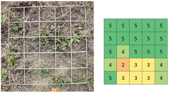
Figure 4.
Example of ground cover assessment using the per-sector-evaluation method [101].
Vegetation in CT consisted mostly of Gramineae. Sorghum halepense was the most recurring species, and to a lesser extent, other botanical families (mainly Fabaceae and Asteraceae) were also observed. Species diversification was more evident during spring and summer, while in autumn and winter, Gramineae took over broad-leaves. In GC, on the other hand, diversification was more evident over the year and, besides the previously mentioned botanical families, Apiaceae, Polygonaceae and Plantaginaceae were also observed. Among the Gramineae, Avena sterilis, Bromus hordeaceus, Cynodon dactylon and Phleum pratense were the most frequently observed in GG. Other broad-leaf species that have been found in both plots are Cirsium arvense, Taraxacum Bellis sp. (Asteraceae), Trifolium repens, Trifolium pratense, Trifolium Fragiferum and Lotus corniculatus (Fabaceae) and Allium vineale (Liliaceae). The effect of non-photosynthetic vegetation (i.e., dead grass and pruning residues) on ground cover assessment proved to be negligible.
2.3.4. Relationship between Ground Cover and Remotely Sensed Data
The data measured in 2014 [60] were used to assess the relationship between inter-row ground cover and cumulated GDDs for each treatment and calibrate the model. The relationship (first-order polynomial linear regression) also considered the reduced growth due to mechanical interventions such as mowing, whose action hinders vegetation growth. The equations obtained for the reference GS for both soil managements were used for the calculation of daily ground cover for our reference period. The aim of this work was to assess the applicability of both S2 native bands and the derived VIs as a proxy to describe the inter-row crop growth throughout the GS, considering different soil managements (tilled or grass-covered). The first-order polynomial linear regression method was used to evaluate the correlation between the two datasets and to define the most suitable type of satellite data for ground cover forecasting. Accuracy and error magnitude was assessed by mean absolute error (MAE):
where is the observation value, and is the corresponding forecast value. MAE, which is the absolute difference between actual and predicted values, can be used to assess the average magnitude of errors, regardless of their direction. Root mean squared error (RMSE) was also considered:
where is the observation value and is the corresponding forecast value. Both metrics can be used to evaluate errors between a set of actual and forecast values, although, in RMSE, the effect of each error is proportional to the size of the squared error. For this reason, RMSE usually has higher values compared to MAE. The two measures can be used together to observe how forecast errors vary, with values ranging from 0 to ∞. Lower values are better, and when the distance between MAE and RMSE increases, the variance between datasets increases as well.
Image processing, intermediate steps, and results for both test areas were managed by free GIS software (QGIS v3.8.0 and SAGA GIS v7.0.0), while statistical analysis and graphical illustration of the results were performed using Python (v3.8).
3. Results and Discussion
3.1. Photointerpretation
With respect to the main goal of this work, an initial analysis was conducted to a wider extent over the vineyards located in the municipalities of Carpeneto and Gavi. These vineyards, which have been previously mapped and characterized, have been used to assess the capability of remotely sensed data to identify the different inter-row soil management. As a result of photointerpretation, it turned out that the most embraced soil management technique involved the adoption of tillage or other mechanical operations, leaving bare soil (CT) in the inter-rows, while vineyards with grass-covered (GC) inter-rows were less common in both analyzed areas. More specifically, in terms of the number of fields, vineyards in both Carpeneto and Gavi with CT management represent 61.6% and 75.7%, respectively, while GC management is less widespread, regarding only 38.4% of the fields in Carpeneto, and 24.3% in Gavi. In terms of area, percentage values are a bit higher for vineyards with GC management, although it still represents the minority of the area in favor of traditional CT management (Table 4). The adoption of techniques leaving bare soil in the inter-rows was traditionally embraced to reduce root competition for soil water resources between vines and spontaneous herbaceous plants. Although, it has been observed that a spontaneous ground cover has positive consequences on soil erosion, water retention, and in some cases, also on grape quality [14,103,104,105,106]. For further analysis, the photointerpretation-derived maps have been rasterized.
Table 4.
Extent of the photointerpreted vineyards in terms of surface (in hectares) and number of fields (i.e., number of polygons) according to soil management (CT = bare soil, GC = grass-cover),and the corresponding percentage value (in italic).
3.2. Soil Management Classification
In satellite imagery, different soil management can be interpreted as a variation of vigor for a specific field or a more widespread area. For vineyards, the signal returned by satellite images is the sum of spectral signatures from different elements (i.e., the main crop, bare or grass-covered soil, and other materials such as pruning residues or stubble that can be found in the inter-rows). For this study, the TS of every VI was analyzed to see whether the spectral response obtained was able to identify variations in soil management. The initial assumption was that higher reflectance values for the TS of every considered VI corresponded to grass-covered vineyards, suggesting a higher biomass content at the field level, while lower reflectance values were assumed to belong to vineyards with less vigor due to the adoption of traditional management practices that tend to leave a bare soil in the inter-rows during the growing season.
Areas were mapped using the unsupervised classification by the K-means clustering algorithm, considering two classes. For each class, the corresponding average trend (Figure 5) was also calculated to correctly interpret the results. The clustering algorithm generated a vigor map (VM) with two classes (or clusters) for both calibration and validation areas (Figure 6 and Figure 7). All VMs presented one cluster with higher and another one with lower reflectance values (hereinafter referred to as clusters 1 and 2, respectively). Differences between the two clusters were less evident during the first part of the agrarian year, probably due to the period of dormancy during winter and the reduced amount of green vegetation within the vineyards until the beginning of spring. Starting in May, differences between clusters usually became more evident when the initial mechanical operations were carried out in the fields (typically, tillage or mowing). From that time on, vine canopies started to expand together with the increase in soil coverage.
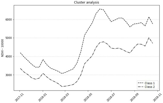
Figure 5.
TS showing the typical average trend (in this case, NDVI) resulting from the unsupervised classification algorithm, distinguishing the vineyards of both wide areas into two classes: Class 1 (higher vigor) and Class 2 (minor vigor). The X-axis indicates the time (year-month).
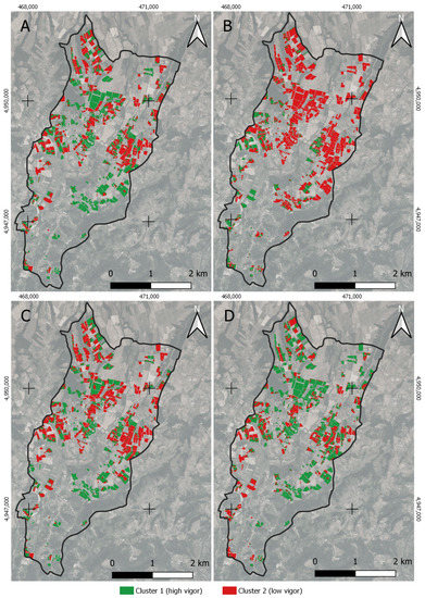
Figure 6.
Cluster analysis of vigor map for the different VIs that have been considered in the calibration area (municipality of Carpeneto): (A) NDVI, (B) NDVIW, (C) NDWI, (D) NDRE.
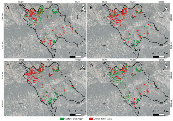
Figure 7.
Cluster analysis vigor map for the validation area (municipality of Gavi) for the different VIs that have been considered: (A) NDVI, (B) NDVIW, (C) NDWI, (D) NDRE.
The unsupervised classification results (Table 5) indicate that traditional indices such as NDVI provided a more balanced distinction between the two managements, slightly in favor of GC (51.9% and 50.4% in Carpeneto and Gavi, respectively) as opposed to CT (>48% in both areas). On the other hand, classification using NDRE was more in favor of GC (>57%), and in detriment of CT (<43%) for both areas. Results from NDWI appeared closer to reference values obtained by photointerpretation, tending to overestimate GC (44.7% and 37.7% in Carpeneto and Gavi, respectively) compared to the reference values obtained using photointerpretation. Regarding the newly proposed index, NDVIW performed poorly in the municipality of Carpeneto, by estimating 80.1% of the study area as vineyards with CT management and underestimating GC. In contrast, NDVIW clustering results appeared to be more like the reference values obtained for the validation area of Gavi.
Table 5.
Differences in extents between areas mapped by photointerpretation, characterized according to inter-rows management, and cluster analysis results for the TS of every considered VI. Clusters follow the same classification criteria indicated in Figure 5. For each class, the first row reports values in hectares, while the second row (in italic) is the equivalent percentage value.
To test clustering results, the obtained VMs were compared to the reference map, where vineyards were identified via photointerpretation (Figure 8 and Figure 9). Accuracy for every considered VI was then evaluated through the metrics that can be derived by the confusion matrix (Table 6). As a matter of fact, the assumption ‘higher reflectance equal higher vigor’ appeared to be true for all the considered VIs to some extent. More specifically, NDVI and NDWI performed better than the others, with more appreciable results for the OA (>0.7) in the calibration area and discrete ones (OA > 0.6) in the validation area. The unsupervised classification method was able to identify with a certain degree of accuracy the differences in soil management, which can be expressed in terms of major or minor vigor observed. NDRE results were appreciable for the calibration area (OA = 0.64), while those were slightly inferior in the validation area (OA = 0.58). At last, among the other VIs that have been considered, NDVIW performed poorly, with OA ≤ 0.6 for both tested areas, showing lesser capabilities in detecting differences between the two clusters.
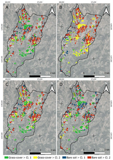
Figure 8.
Results of the comparison between the reference map and the results of the cluster analysis in the calibration area (municipality of Carpeneto) for the different VIs that have been considered: (A) NDVI, (B) NDVIW, (C) NDWI, (D) NDRE.
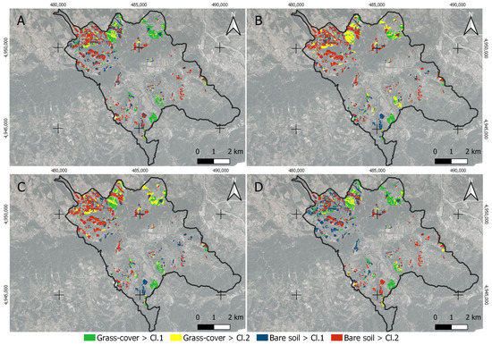
Figure 9.
Results of the comparison between the reference map and the results of the cluster analysis in the validation area (municipality of Gavi) for the different VIs that have been considered: (A) NDVI, (B) NDVIW, (C) NDWI, (D) NDRE.
Table 6.
Results of the confusion matrix. Class 1 refers to the pixels that have been classified as vineyards (or portions of them) with higher vigor and, therefore, interpreted as grass-covered inter-rows, while Class 2 includes vineyards with a minor vigor, supposedly having bare soil in the inter-rows during the growing season.
Among the other accuracy metrics, producer and user accuracy (PA and UA, respectively) presented a higher variability for every analyzed index. As well as for the OA, NDVI reported the best results in both areas compared to the other VIs. Above all, PA scored the best values (0.84 both in Carpeneto and Gavi) for the identification of pixels belonging to Class 2 (lower vigor), while PA for Class 1 (higher vigor) was mediocre (≤0.65). According to these results, the classifier was more able to detect vineyards (or parts of them) with traditional inter-row soil management. Similar behavior was observed for the other indices, with appreciable results predicting Class 2 using NDWI and NDRE (PA > 0.7), while NDVIW provided the lowest results for both areas (PA < 0.7). In a similar way, PA was quite low (<0.7) predicting Class 1 pixels. UA, on the other hand, reported higher values in Class 1 (UA > 0.8 in Carpeneto and >0.7 in Gavi) for NDVI and NDRE, while discrete results for UA in Class 2 (≥0.7) were obtained by NDWI and NDVIW.
Regarding the surface variations highlighted by the confusion matrix (Table 7), the cluster analysis appeared to be less accurate in identifying vineyards (or portions of them) belonging to Cluster 1 (i.e., higher vigor), although NDVI and NDWI had more than 64% of the area that was correctly identified, and to a lesser extent, NDRE performed moderately as well (>50%), while lower results were those provided by NDVIW (<40%) for the municipality of Carpeneto. Results in Gavi were slightly inferior at identifying Cluster 1, but all VIs performed similarly, matching the reference map and the corresponding cluster map (GC_Cl1) ranging from 42 to 52%. Even in Gavi, NDVI gave the best results (52.5%). For the identification of pixels belonging to Cluster 2 (i.e., lower vigor), matching results (CT_Cl2) indicated a better capability of all considered VIs in identifying the pixels correctly. In fact, results in both areas for the traditional VIs were almost 85% in NDVI, and higher than 70% for both NDWI and NDRE. Even in this case, only NDVIW exhibited lower results (<70%). This difference between the two test areas may be related to factors affecting the capability of VIs to identify the different soil management, especially regarding the newly proposed NDVIW. Further studies may be moving towards a better definition of this modified version of the traditional NDVI formula.
Table 7.
Difference in extents between the reference classification and the confusion matrix (combination of reference map and classification results for every tested VI). For each combination, the first row reports values in hectares, while the second row (in italic) is the equivalent percentage value.
Results suggested that the bands in the red and infrared regions combined in the tested VIs may be able to detect variations in terms of soil coverage, especially in the red and NIR and, to some extent, in the red-edge and SWIR as well. The NIR has some advantages for the detection and assessment of vegetation canopies since a higher amount of light is reflected in this region (50–60%) compared to that reflected in the blue, green, or red (2%, 5%, and 3% respectively) for vegetation canopy [107]. Since NIR is a combined function of leaf optical properties, canopy geometry, and soil reflectance [108], it is also able to reflect the soil, which is characterized by lower reflectance values compared to vegetation signals.
In this research, VIs including the NIR band in their formula displayed the best results and respected the assumption that the higher vigor class observed could have been attributed to grass-covered vineyards, while lower values were related to a minor vegetation density, typical of vineyards managed in a traditional way, leaving bare soil or scarce spontaneous vegetation growing in the inter-rows. The SWIR spectral region is used instead for different applications, such as distinguishing cloud types and estimating water content in soils and plants. Although classification proved to be able to identify variations in vineyards, accuracy values were usually lower than those obtained by NDVI.
A consideration must be made: the classification performed by the operator generated a map in which the single field was classified in its whole, referring to a precise time of the year when the orthophotos were taken. The automatic classification, on the other hand, was pixel-based, distinguishing different portions within the field and identifying the areas with greater vegetation and those where the vegetation (whether vine plants or the vegetation in the inter-row) growth was stunted. This may be one of the reasons explaining the fact that producer and user accuracy presented differences for the same class since the reference map is a simplification of the reality observed on the ground, considering the vineyard as a whole without regard to the spatial variations that occur during the GS. Despite the reduced geometric resolution of the S2 data, the use of cluster analysis was able to highlight the differences in vigor within every field. This spatial variability was probably due to both the different vigor of vine growth and the presence of spontaneous herbaceous plants growing into the fields as well. Thus, vineyards that in the reference map were originally classified with tilled inter-rows presented spots with higher vegetation that had been classified as grass-vegetated areas by the unsupervised classification. Oppositely, vineyards identified as having grass-covered inter-rows could have presented sparse vegetation in some portions of the field, especially in the middle or along the boundaries.
3.3. Ground Cover Assessment
In addition to the wide-area analysis, we also investigated data collected at the plot level in the Tenuta Cannona vineyards. Traditionally, the CT plot was managed by leaving bare soil during the GS, undergoing two tillage operations: one at the beginning of spring, and wintry tillage right after harvest time. Oppositely, the GC plot underwent no tillage at all, and the only mechanical operations carried out during the GS were mowing, vine topping, and phytosanitary treatments. At the beginning of the GS, before the first proper vernal soil processing, pruning residues were shredded, and diseased vine plants were removed at the end of March in both plots. According to the data collected by Repullo et al. [60], and given the similar climatic trend between both years, the model developed in 2014 to estimate ground cover based on GDDs was used for our reference period. The model highlighted a first-order polynomial linear regression between ground cover measurements and GDDs, with high values for both experimental plots (0.98 for GC and 0.90 for CT). That led to the assumption that it was possible to estimate ground cover development based on climatic parameters such as temperature (involved in GDDs calculation) and knowing the influence of mechanical operations on inter-row development. More specifically, to simulate the effect of mowing, a 7% reduction in the daily ground cover calculation was applied when those operations were carried out during the 2018 GS. Regarding tillage operations, which determined the removal of all ground cover from the inter-rows, the effect was replicated by setting the GDD value back to 0 to the corresponding operation date. The resulting data of the ground cover assessment have been used to evaluate the relations between ground cover measurements and remotely sensed data (Table 8 and Figure A1, Figure A2 and Figure A3).
Table 8.
First-order polynomial linear regression results * (expressed by the coefficient of determination, ) between ground cover (%) and reflectance data for every S2 native band and vegetation index. Error metrics (MAE and RMSE) are also reported for every considered time interval: (i) Tot. regards the entire agrarian year (November 2017–October 2018), while parts one and two range from (ii) November 2017 to April 2018 and (iii) from May 2017 to October 2018, respectively.
3.4. Relationship between Ground Cover and Remotely Sensed Data
The capability of VIs to provide information regarding vegetation cover, vigor, and growth dynamics [76,109,110] is known, although other studies showed that such information could be obtained using native bands provided by satellites in different spectral regions as well [111,112,113]. With this in mind, we aimed to assess the capability of both VIs and S2 native bands to describe the inter-row degree of coverage taking place within the vineyards with different soil management. Once the ground cover was estimated, a further analysis was carried out to evaluate if the S2 native bands and the considered VIs were able to describe the degree of vegetation cover within the inter-rows based on the different types of soil management during the reference period (agrarian year 2017–2018). To do so, the regression between the TS for every piece of satellite data (either S2 native bands or the derived VIs) and inter-row’s ground cover estimation was calculated considering different time intervals. In the first case, the agrarian year was analyzed as a whole. The TS was then split into two parts to test the regression results and evaluate the presence of a seasonality effect.
The first part considered the period ranging from November 2017 until the end of April 2018, when the first tillage or mowing operations were carried out in CT and GC plots, respectively. During this time interval, it is assumed that the vines are in the vegetative rest phase, with no (or very low) green canopy, and therefore have a reduced influence or almost nothing on the reflectance signal recorded by the Sentinel-2 sensors. Having made this assumption, values in the different spectral regions and VIs originated almost exclusively from the spontaneous vegetation growing in the inter-rows of the vineyards.
The second time interval instead ranged from the beginning of May, after tillage or mowing (based on the different soil management per experimental plot), and lasted until the end of the agrarian reference period in October 2018. During this second period, vine canopies kept growing over time, supposedly affecting the capability of remotely sensed data to describe inter-rows coverage development. From the end of April to early May, however, we assumed that the signal relating to the degree of coverage of the inter-rows was also influenced by that of the developing vine plants until the senescence phase took place in autumn. For these time intervals, first-order polynomial linear regression was calibrated to assess the correspondence between the two datasets and to verify the presence of a “seasonality effect”. Error assessment was also measured considering MAE and RMSE (Table 8). The aim was to identify the most suitable band or index to describe inter-rows vegetative growth in relation to the different periods of the year. Appreciable results were those whose coefficient of determination reported values higher than 0.7.
For both plots, first-order polynomial linear regression showed lower results when the entire reference period was considered (Figure A1). More specifically, all S2 native bands performed poorly ( < 0.2), and similarly, VIs had low values but were characterized by higher variability within the results. Only NDVI scored = 0.61 and 0.43 for CT and GC, respectively. To some extent, the NDVI was the only index that showed, in the long term and on vineyards with tilled inter-rows, a good predictive capability of the coverage degree. Gaps between MAE and RMSE were considerable, suggesting a high variability within the datasets, especially for the GC plot. However, taking into consideration the two intervals separately, the results changed.
During the first part of the reference period (Figure A2), S2 native bands, and more in detail, those recorded in the visible, displayed a very high coefficient of determination ( ≥ 0.9 in CT and >0.8 in GC). The bands ranging from the red-edge to the SWIR regions highlighted lower values, but the results were satisfactory nevertheless. CT coefficients were higher (≥ 0.75) compared to those recorded for GC (≥ 0.6). The best records for both CT and GC in the red-edge band were obtained by B5 ( = 0.87 and 0.78 for CT and GC, respectively), with good results given by the NIR band for CT ( = 0.83), while values for GC were the lowest among the native bands ( = 0.6). In a similar way, SWIR bands gave good results for both plots, suggesting that further analysis on these bands could be carried out. Regarding the VIs, results obtained for CT indicated that all tested indices were able to predict ground cover in tilled vineyards in a suitable way, while results for GC displayed a higher variability, highlighting the importance of choosing the most fitted index to describe inter-row vegetation development based on soil management adopted within the vineyard. In the same way, gaps in MAE and RMSE values were smaller in CT compared to those in GC, and as a reflection of results, those gaps were higher for GC vegetation indices. More specifically, NDRE performed better than the other indices both in CT and GC ( = 0.77 and 0.78, respectively), while NDVI obtained the worst result in GC ( = 0.10). The newly proposed index NDVIW, on the other hand, performed very well in CT ( = 0.77) and reported a decent value in GC ( = 0.52). Oppositely, NDVI and NDWI reported the worst coefficient values ( < 0.3) in this first timescale.
After mechanical operations in spring, when soil tillage in CT and the first mowing in GC in the inter-rows were carried out, the influence of the growing vine canopies on the signal detected by satellite sensors increased over the season. That determined a reduction in the accuracy of inter-row cover assessment in the second part of the GS (Figure A3). Since the satellite sensors’ reflectance signal also started being influenced and describing the growth dynamics of the vine plants, values were affected in a variable manner according to the different spectral band that is taken into analysis. Like in the previous timescales, values were higher in CT other than in GC. Among the spectral bands, the best responses for both plots had been observed in the green (B3, = 0.76 and 0.69 for CT and GC, respectively) and red-edge bands. Regarding the red-edge bands, B5 and B6 performed better in CT (≥ 0.7), while growth dynamics in GC were best described by B6 and B7 (≥ 0.7). Values in the NIR band as well were appreciable for the GC plot ( = 0.74), while the coefficient was reduced in CT ( = 0.64). Apart from that, results for both SWIR bands returned appreciable results for neither considered management, even though the NDWI performed better among all VIs for the CT plot ( = 0.73), while values decreased significantly in GC ( = 0.22). Similar behavior was observed for NDRE ( = 0.68 and 0.51 for CT and GC, respectively). While NDVI reported the lowest values in both cases ( < 0.3), NDVIW results were quite low but still noticeable (≥ 0.4). In this phase, VIs, in general, proved less suitable than the previous time interval to describe the evolution of ground cover.
4. Conclusions
Information regarding vineyard management is usually hard to find and may require in-field measurements. The adoption of techniques such as unsupervised classification of remotely sensed data for a given period can be a useful and time-saving tool, allowing the users to characterize a specific area without the need to create a training set (required for supervised classification methods). In this work, results from the cluster analysis suggested that open-source satellite data, despite being characterized by a geometrical resolution that does not allow to discriminate between vine rows and inter-rows, can be useful to determine the differences in terms of soil management of the latter part of the vineyard. Open-source data such as Sentinel-2 are, in fact, characterized by a high temporal frequency, allowing the user to reconstruct growth dynamics within the vineyard that may be related either to the vine plants or the ground cover that can be found in the inter-rows. That way, cluster analysis can provide information about the vigor differences taking place within a vineyard both from the spatial and temporal point of view, allowing one to distinguish portions of the field with different vigor. That could be due to the presence of vine plants that failed to grow rather than the presence of portions of bare soil in the inter-rows, both indicators of incorrect management practices. Information of this type can be useful for crop monitoring purposes using satellite sensors.
Regarding plot-level analysis, growth dynamics taking place within the inter-rows can be identified either by different vegetation indices or the Sentinel-2 native bands as well. This can be applied both in vineyards having bare soil or grass-covered inter-rows. Regression analysis between remotely sensed data and estimated ground cover highlights differences between the values obtained for the entire growing season compared to those for the split time intervals. Higher values observed in the split time intervals indicate that there is a seasonality effect that may determine the choice of a specific index or spectral band, being more able to describe the development of vegetation cover based on the time of the year we are taking in consideration and the different soil management that can be applied into the vineyard. The choice of a different predictive model at a certain point of the growing season suggests that, at some point, the main crop begins to prevail in the reflectance signal detected, making it more difficult to estimate the coverage of the inter-rows. In general, the joint use of different vegetation indices is desirable to better evaluate the evolution of the biomass within the field and the variation of the relationship between row and inter-row. On this matter, results obtained by the newly proposed NDVIW for the split reference periods suggest that weighing the index to best evaluate only one of the components within the vineyard (either main row-crop or inter-rows) might be working. The idea is that the index might work well when there are low densities of vegetation within the field (e.g., bare soil or low vegetation in the inter-rows), while when different vegetation sources at different dimensional levels are present, the use of an index containing reflectance values in the red-edge band (NDRE) might be more useful for describing coverage development. Further analyses and tests on time series of bands in different spectral regions are required to find the best formula for a weighted index able to describe ground cover development of the service crop. Such type of data may find applicability in predictive models for the estimation of crop growth, water balance, or erosive phenomena.
Author Contributions
Conceptualization: F.P., E.C.B.M. and M.B.; methodology and validation: E.C.B.M. and M.B.; data curation: F.P.; writing—original draft preparation: F.P.; writing—review and editing: E.C.B.M. and M.B.; supervision: M.B. and E.C.B.M.; project administration: E.C.; funding acquisition: E.C. All authors have read and agreed to the published version of the manuscript.
Funding
This research was funded by the Fondazione Giovanni Goria and Fondazione CRT (Bando Talenti della Società Civile 2020). Part of this research was also carried out within the framework of the IN-GEST SOIL Project, funded by the Rural Development 2014–2020 for Operational Groups (in the sense of Art 56 of Reg.1305/2013).
Data Availability Statement
Technical maps of the study area were obtained from the open Official Geoportal of the Piemonte Region Administration (http://www.geoportale.piemonte.it/ (accessed on 8 June 2022)), while remotely sensed data from Sentinel-2 mission were collected and processed in Google Earth Engine (https://developers.google.com/earth-engine/datasets/ (accessed on 8 June 2022)).
Conflicts of Interest
The authors declare no conflict of interest. The funders had no role in the design of the study; in the collection, analyses, or interpretation of data; in the writing of the manuscript; or in the decision to publish the results.
Appendix A
First-order polynomial linear regression between remotely sensed data (on the X-axis) and ground cover percentage (on the Y-axis) for the entire first and second part of the reference period. The corresponding equation for every plot is reported in the legend, while values are reported next to every trend line.

Figure A1.
First-order polynomial linear regression between remotely sensed data (X-axis) and ground cover percentage (Y-axis) for the entire reference period.

Figure A2.
First-order polynomial linear regression between remotely sensed data (X-axis) and ground cover percentage (Y-axis) for the first part of the reference period.

Figure A3.
First-order polynomial linear regression between remotely sensed data (X-axis) and ground cover percentage (Y-axis) for the second part of the reference period.
References
- OIV. OIV General Principles of Sustainable Vitiviniculture—Environmental—Social—Economic and Cultural Aspects; OIV: Paris, France, 2016. [Google Scholar]
- CEC. Proposal for a Directive of the European Parliament and of the Council: Establishing a Framework for Greenhouse Gas Emissions Trading within the European Community: An Analysis of Some Salient Elements; European Union: Luxembourg, 2001. [Google Scholar]
- CEC. Communication from the Commission to the Council, the European Parliament, the European Economic and Social Committee and the Committee of the Regions: Civil Society Dialogue Between the EU and Candidate Countries; Commission of the European Communities: Brussels, Belgium, 2005; Volume 290. [Google Scholar]
- FAO. Status of the World’s Soil Resources—Main Report; FAO, ITPS: Rome, Italy, 2015; OCLC: 945442780. [Google Scholar]
- CEC. EU Soil Strategy for 2030—Reaping the Benefits of Healthy Soils for People, Food, Nature and Climate; European Union: Luxembourg, 2021. [Google Scholar]
- Martucci, O.; Arcese, G.; Montauti, C.; Acampora, A. Social Aspects in the Wine Sector: Comparison between Social Life Cycle Assessment and VIVA Sustainable Wine Project Indicators. Resources 2019, 8, 69. [Google Scholar] [CrossRef]
- Dunbar, M.B.; Panagos, P.; Montanarella, L. European perspective of ecosystem services and related policies. Integr. Environ. Assess. Manag. 2013, 9, 231–236. [Google Scholar] [CrossRef] [PubMed]
- Cerqueira, Y.; Navarro, L.M.; Maes, J.; Marta-Pedroso, C.; Pradinho Honrado, J.; Pereira, H.M. Ecosystem Services: The Opportunities of Rewilding in Europe. In Rewilding European Landscapes; Pereira, H.M., Navarro, L.M., Eds.; Springer International Publishing: Cham, Switzerland, 2015; pp. 47–64. [Google Scholar] [CrossRef]
- Montanaro, G.; Xiloyannis, C.; Nuzzo, V.; Dichio, B. Orchard management, soil organic carbon and ecosystem services in Mediterranean fruit tree crops. Sci. Hortic. 2017, 217, 92–101. [Google Scholar] [CrossRef]
- Gómez, J.A. Sustainability using cover crops in Mediterranean tree crops, olives and vines – Challenges and current knowledge. Hung. Geogr. Bull. 2017, 66, 13–28. [Google Scholar] [CrossRef]
- Winter, S.; Bauer, T.; Strauss, P.; Kratschmer, S.; Paredes, D.; Popescu, D.; Landa, B.; Guzmán, G.; Gómez, J.A.; Guernion, M.; et al. Effects of vegetation management intensity on biodiversity and ecosystem services in vineyards: A meta-analysis. J. Appl. Ecol. 2018, 55, 2484–2495. [Google Scholar] [CrossRef] [PubMed]
- Garcia, L.; Celette, F.; Gary, C.; Ripoche, A.; Valdés-Gómez, H.; Metay, A. Management of service crops for the provision of ecosystem services in vineyards: A review. Agric. Ecosyst. Environ. 2018, 251, 158–170. [Google Scholar] [CrossRef]
- Ferreira, C.S.S.; Keizer, J.J.; Santos, L.M.B.; Serpa, D.; Silva, V.; Cerqueira, M.; Ferreira, A.J.D.; Abrantes, N. Runoff, sediment and nutrient exports from a Mediterranean vineyard under integrated production: An experiment at plot scale. Agric. Ecosyst. Environ. 2018, 256, 184–193. [Google Scholar] [CrossRef]
- Bagagiolo, G.; Biddoccu, M.; Rabino, D.; Cavallo, E. Effects of rows arrangement, soil management, and rainfall characteristics on water and soil losses in Italian sloping vineyards. Environ. Res. 2018, 166, 690–704. [Google Scholar] [CrossRef]
- López-Vicente, M.; Gómez, J.A.; Guzmán, G.; Calero, J.; García-Ruiz, R. The role of cover crops in the loss of protected and non-protected soil organic carbon fractions due to water erosion in a Mediterranean olive grove. Soil Tillage Res. 2021, 213, 105119. [Google Scholar] [CrossRef]
- FAO. 2019. Available online: https://www.fao.org/faostat/en/#data/QCL (accessed on 20 October 2022).
- ISTAT. 2019. Available online: https://www.istat.it/it/agricoltura (accessed on 20 October 2022).
- IPLA. Carta dell’Erosione Reale del Suolo; IPLA: Liverpool, UK, 2009. [Google Scholar]
- Heege, H.J. Precision in Crop Farming. Site Specific Concepts and Sensing Methods: Applications and Results; Springer: Berlin/Heidelberg, Germany, 2015; OCLC: 925497917. [Google Scholar]
- Towers, P.C.; Strever, A.; Poblete-Echeverría, C. Comparison of Vegetation Indices for Leaf Area Index Estimation in Vertical Shoot Positioned Vine Canopies with and without Grenbiule Hail-Protection Netting. Remote Sens. 2019, 11, 1073. [Google Scholar] [CrossRef]
- Sort, X.; Ubalde, J.M. Aspectos de viticultura de precisión en la práctica de la fertilización razonada. In ACE: Revista de Enología; Rubes Editorial: Barcelona, Spain, 2005. [Google Scholar]
- Da Silva, A.; Sinfort, C.; Tinet, C.; Pierrat, D.; Huberson, S. A Lagrangian model for spray behaviour within vine canopies. J. Aerosol Sci. 2006, 37, 658–674. [Google Scholar] [CrossRef]
- Campos, J.; Llop, J.; Gallart, M.; García-Ruiz, F.; Gras, A.; Salcedo, R.; Gil, E. Development of canopy vigour maps using UAV for site-specific management during vineyard spraying process. Precis. Agric. 2019, 20, 1136–1156. [Google Scholar] [CrossRef]
- Testa, S.; Mondino, E.C.B.; Pedroli, C. Correcting MODIS 16-day composite NDVI time-series with actual acquisition dates. Eur. J. Remote Sens. 2014, 47, 285–305. [Google Scholar] [CrossRef]
- Borgogno-Mondino, E.; Lessio, A.; Tarricone, L.; Novello, V.; de Palma, L. A comparison between multispectral aerial and satellite imagery in precision viticulture. Precis. Agric. 2017, 19, 195–217. [Google Scholar] [CrossRef]
- Corvino, G.; Lessio, A.; Borgogno-Mondino, E. Monitoring Rice Crops in Piemonte (Italy): Towards an Operational Service Based on Free Satellite Data. In Proceedings of the IGARSS 2018-2018 IEEE International Geoscience and Remote Sensing Symposium, Valencia, Spain, 22–27 July 2018; pp. 9070–9073. [Google Scholar] [CrossRef]
- De Petris, S.; Berretti, R.; Sarvia, F.; Borgogno-Mondino, E. Precision arboriculture: A new approach to tree risk management based on geomatics tools. Int. Soc. Opt. Photonics 2019, 11149, 111491G. [Google Scholar] [CrossRef]
- Sarvia, F.; De Petris, S.; Borgogno-Mondino, E. Remotely sensed data to support insurance strategies in agriculture. Int. Soc. Opt. Photonics 2019, 11149, 111491H. [Google Scholar] [CrossRef]
- Hall, A.; Louis, J.; Lamb, D. Characterising and mapping vineyard canopy using high-spatial-resolution aerial multispectral images. Comput. Geosci. 2003, 29, 813–822. [Google Scholar] [CrossRef]
- Ferreiro-Armán, M.; Da Costa, J.P.; Homayouni, S.; Martín-Herrero, J. Hyperspectral Image Analysis for Precision Viticulture; Lecture Notes in Computer Science; Springer: Berlin/Heidelberg, Germany, 2006; pp. 730–741. [Google Scholar] [CrossRef]
- Arnó, J.; Martínez Casasnovas, J.A.; Ribes Dasi, M.; Rosell, J.R. Review. Precision Viticulture. Research Topics, Challenges and Opportunities in Site-Specific Vineyard Management; Instituto Nacional de Investigación y Tecnología Agraria y Alimentaria: Madrid, Spain, 2009. [Google Scholar] [CrossRef]
- Hall, A.; Wilson, M.A. Object-based analysis of grapevine canopy relationships with winegrape composition and yield in two contrasting vineyards using multitemporal high spatial resolution optical remote sensing. Int. J. Remote Sens. 2013, 34, 1772–1797. [Google Scholar] [CrossRef]
- Karakizi, C.; Oikonomou, M.; Karantzalos, K. Vineyard Detection and Vine Variety Discrimination from Very High Resolution Satellite Data. Remote Sens. 2016, 8, 235. [Google Scholar] [CrossRef]
- Hall, A. Remote Sensing Applications for Viticultural Terroir Analysis. Elements 2018, 14, 185–190. [Google Scholar] [CrossRef]
- Rouse, J.W.; Haas, R.H.; Deering, D.W.; Schell, J.A. Monitoring the Vernal Advancement and Retrogradation (Green Wave Effect) of Natural Vegetation. [Great Plains Corridor]; Technical report; NASA: Washingtong, DC, USA, 1974. [Google Scholar]
- Huete, A.R. A soil-adjusted vegetation index (SAVI). Remote Sens. Environ. 1988, 25, 295–309. [Google Scholar] [CrossRef]
- Qi, J.; Chehbouni, A.; Huete, A.R.; Kerr, Y.H.; Sorooshian, S. A modified soil adjusted vegetation index. Remote Sens. Environ. 1994, 48, 119–126. [Google Scholar] [CrossRef]
- Gao, B.c. NDWI—A normalized difference water index for remote sensing of vegetation liquid water from space. Remote Sens. Environ. 1996, 58, 257–266. [Google Scholar] [CrossRef]
- Motohka, T.; Nasahara, K.N.; Oguma, H.; Tsuchida, S. Applicability of Green-Red Vegetation Index for Remote Sensing of Vegetation Phenology. Remote Sens. 2010, 2, 2369–2387. [Google Scholar] [CrossRef]
- Smart, R.E. Principles of Grapevine Canopy Microclimate Manipulation with Implications for Yield and Quality. A Review. Am. J. Enol. Vitic. 1985, 36, 230–239. [Google Scholar]
- Haselgrove, L.; Botting, D.; Heeswijck, v.R.; Høj, P.B.; Dry, P.R.; Ford, C.; Land, P.G.I. Canopy microclimate and berry composition: The effect of bunch exposure on the phenolic composition of Vitis vinifera L cv. Shiraz grape berries. Aust. J. Grape Wine Res. 2000, 6, 141–149. [Google Scholar] [CrossRef]
- Petrie, P.R.; Trought, M.C.T.; Howell, G.S. Fruit composition and ripening of Pinot Noir (Vitis vinifera L.) in relation to leaf area. Aust. J. Grape Wine Res. 2000, 6, 46–51. [Google Scholar] [CrossRef]
- Hall, A.; Lamb, D.W.; Holzapfel, B.; Louis, J. Optical remote sensing applications in viticulture—A review. Aust. J. Grape Wine Res. 2002, 8, 36–47. [Google Scholar] [CrossRef]
- Matese, A.; Toscano, P.; Di Gennaro, S.F.; Genesio, L.; Vaccari, F.P.; Primicerio, J.; Belli, C.; Zaldei, A.; Bianconi, R.; Gioli, B. Intercomparison of UAV, Aircraft and Satellite Remote Sensing Platforms for Precision Viticulture. Remote Sens. 2015, 7, 2971–2990. [Google Scholar] [CrossRef]
- Matese, A.; Di Gennaro, S.F. Technology in precision viticulture: A state of the art review. Int. J. Wine Res. 2015, 7, 69–81. [Google Scholar] [CrossRef]
- Borgogno-Mondino, E.; de Palma, L.; Novello, V. Investigating Sentinel 2 Multispectral Imagery Efficiency in Describing Spectral Response of Vineyards Covered with Plastic Sheets. Agronomy 2020, 10, 1909. [Google Scholar] [CrossRef]
- Celette, F.; Findeling, A.; Gary, C. Competition for nitrogen in an unfertilized intercropping system: The case of an association of grapevine and grass cover in a Mediterranean climate. Eur. J. Agron. 2009, 30, 41–51. [Google Scholar] [CrossRef]
- Abazi, U.; Lorite, I.J.; Cárceles, B.; Martínez Raya, A.; Durán, V.H.; Francia, J.R.; Gómez, J.A. WABOL: A conceptual water balance model for analyzing rainfall water use in olive orchards under different soil and cover crop management strategies. Comput. Electron. Agric. 2013, 91, 35–48. [Google Scholar] [CrossRef]
- Simionesei, L.; Oliveira, A.; Ramos, T.; Neves, R. Modelação da rega deficitária em vinha com o MOHID-Land. In Proceedings of the X Congreso Ibérico de Agroingeniería, Huesca, Spain, 3–6 September 2019. Number: COMPON-2019-agri-3373. [Google Scholar] [CrossRef]
- Pinto, V.M.; van Dam, J.C.; de Jong van Lier, Q.; Reichardt, K. Intercropping Simulation Using the SWAP Model: Development of a 2×1D Algorithm. Agriculture 2019, 9, 126. [Google Scholar] [CrossRef]
- Ippolito, M.; Minacapilli, M.; Provenzano, G. Combining the FAO56 agrohydrological model and remote sensing data to assess water demand in a Sicilian irrigation district. In Proceedings of the 22nd EGU General Assembly, Vienna, Austria, 4–8 May 2020. [Google Scholar] [CrossRef]
- Darouich, H.; Ramos, T.B.; Pereira, L.S.; Rabino, D.; Bagagiolo, G.; Capello, G.; Simionesei, L.; Cavallo, E.; Biddoccu, M. Water Use and Soil Water Balance of Mediterranean Vineyards under Rainfed and Drip Irrigation Management: Evapotranspiration Partition and Soil Management Modelling for Resource Conservation. Water 2022, 14, 554. [Google Scholar] [CrossRef]
- Andreoli, R. Modeling Erosion Risk Using the RUSLE Equation. In QGIS and Applications in Water and Risks; John Wiley & Sons, Ltd.: Hoboken, NJ, USA, 2018; pp. 245–282. [Google Scholar] [CrossRef]
- Gómez, J.A.; Biddoccu, M.; Guzmán, G. ORUSCAL: RUSLE Calculator for Orchards; Digital CSIC: Madrid, Spain, 2020. [Google Scholar] [CrossRef]
- Capello, G.; Biddoccu, M.; Simionesei, L.; Ramos, T.; Oliveira, A.; Grosso, N.; Podder, P.; Rabino, D.; Bagagiolo, G.; Neves, R. Use of Mohid-Land to model water balance for implementation of deficit irrigation in vineyards. In Proceedings of the 22nd EGU General Assembly, Vienna, Austria, 4–8 May 2020. [Google Scholar] [CrossRef]
- Biddoccu, M.; Guzmán, G.; Capello, G.; Thielke, T.; Strauss, P.; Winter, S.; Zaller, J.G.; Nicolai, A.; Cluzeau, D.; Popescu, D.; et al. Evaluation of soil erosion risk and identification of soil cover and management factor (C) for RUSLE in European vineyards with different soil management. Int. Soil Water Conserv. Res. 2020, 8, 337–353. [Google Scholar] [CrossRef]
- Borrelli, P.; Alewell, C.; Alvarez, P.; Anache, J.A.A.; Baartman, J.; Ballabio, C.; Bezak, N.; Biddoccu, M.; Cerdà, A.; Chalise, D.; et al. Soil erosion modelling: A global review and statistical analysis. Sci. Total Environ. 2021, 780, 146494. [Google Scholar] [CrossRef]
- Rizzi, J.; Tarquis, A.M.; Gobin, A.; Semenov, M.; Zhao, W.; Tarolli, P. Preface: Remote sensing, modelling-based hazard and risk assessment, and management of agro-forested ecosystems. Nat. Hazards Earth Syst. Sci. 2021, 21, 3873–3877. [Google Scholar] [CrossRef]
- Beniaich, A.; Silva, M.L.N.; Guimarães, D.V.; Avalos, F.A.P.; Terra, F.S.; Menezes, M.D.; Avanzi, J.C.; Cândido, B.M. UAV-based vegetation monitoring for assessing the impact of soil loss in olive orchards in Brazil. Geoderma Reg. 2022, 30, e00543. [Google Scholar] [CrossRef]
- Repullo, M.A.; Opsi, F.; Biddoccu, M.; Cavallo, E. Study on Cover Crop Evolution and Residue/Cover in Vineyard Inter-Rows. Technical Report. 2014. Available online: https://publications.cnr.it/doc/282524 (accessed on 8 November 2022).
- Kottek, M.; Grieser, J.; Beck, C.; Rudolf, B.; Rubel, F. World Map of the Köppen-Geiger climate classification updated. Meteorol. Z. 2006, 259–263. [Google Scholar] [CrossRef]
- Rubel, F.; Kottek, M. Observed and projected climate shifts 1901-2100 depicted by world maps of the Köppen-Geiger climate classification. Meteorol. Z. 2010, 135–141. [Google Scholar] [CrossRef]
- USDA. Keys to Soil Taxonomy, 11th ed.; United States Department of Agriculture, Natural Resources Conservation Service: Washington, DC, USA, 2010; OCLC: 880746518.
- d’Italia, S.G. Carta Geologica d’Italia a Scala 1:100000, Foglio 70 (Alessandria); ISPRA: Alessandria, Italy, 1969. [Google Scholar]
- FAO; ISRIC; ISSS. World Reference Base for Soil Resources; FAO: Rome, Italy, 1998; OCLC: 704183030. [Google Scholar]
- Capello, G.; Biddoccu, M.; Cavallo, E. Permanent cover for soil and water conservation in mechanized vineyards: A study case in Piedmont, NW Italy. Ital. J. Agron. 2020, 15, 323–331. [Google Scholar] [CrossRef]
- ESA. Sentinel-2 User Handbook; ESA: Paris, France, 2015. [Google Scholar]
- Gascon, F.; Bouzinac, C.; Thépaut, O.; Jung, M.; Francesconi, B.; Louis, J.; Lonjou, V.; Lafrance, B.; Massera, S.; Gaudel-Vacaresse, A.; et al. Copernicus Sentinel-2A Calibration and Products Validation Status. Remote Sens. 2017, 9, 584. [Google Scholar] [CrossRef]
- Louis, J.; Charantonis, A.; Berthelot, B. Cloud Detection for Sentinel-2. In Proceedings of the ESA Living Planet Symposium, Bergen, Norway, 28 June–2 July 2010. [Google Scholar]
- Main-Knorn, M.; Pflug, B.; Louis, J.; Debaecker, V.; Müller-Wilm, U.; Gascon, F. Sen2Cor for sentinel-2. Int. Soc. Opt. Photonics 2017, 10427, 1042704. [Google Scholar]
- Gorelick, N.; Hancher, M.; Dixon, M.; Ilyushchenko, S.; Thau, D.; Moore, R. Google Earth Engine: Planetary-scale geospatial analysis for everyone. Remote Sens. Environ. 2017, 202, 18–27. [Google Scholar] [CrossRef]
- Amani, M.; Ghorbanian, A.; Ahmadi, S.A.; Kakooei, M.; Moghimi, A.; Mirmazloumi, S.M.; Moghaddam, S.H.A.; Mahdavi, S.; Ghahremanloo, M.; Parsian, S.; et al. Google Earth Engine Cloud Computing Platform for Remote Sensing Big Data Applications: A Comprehensive Review. IEEE J. Sel. Top. Appl. Earth Obs. Remote Sens. 2020, 13, 5326–5350. [Google Scholar] [CrossRef]
- Borgogno-Mondino, E.; Lessio, A. A FFT-Based Approach to Explore Periodicity of Vines/Soil Properties in Vineyard from Time Series of Satellite-Derived Spectral Indices. In Proceedings of the IGARSS 2018—2018 IEEE International Geoscience and Remote Sensing Symposium, Valencia, Spain, 22–27 July 2018; pp. 9078–9081. [Google Scholar] [CrossRef]
- Savitzky, A.; Golay, M.J.E. Smoothing and Differentiation of Data by Simplified Least Squares Procedures. Anal. Chem. 1964, 36, 1627–1639. [Google Scholar] [CrossRef]
- Jin, H.; Eklundh, L. A physically based vegetation index for improved monitoring of plant phenology. Remote Sens. Environ. 2014, 152, 512–525. [Google Scholar] [CrossRef]
- Xue, J.; Su, B. Significant Remote Sensing Vegetation Indices: A Review of Developments and Applications. J. Sens. 2017, 2017, e1353691. [Google Scholar] [CrossRef]
- Bannari, A.; Morin, D.; Bonn, F.; Huete, A.R. A review of vegetation indices. Remote Sens. Rev. 1995, 13, 95–120. [Google Scholar] [CrossRef]
- Huete, A.; Didan, K.; Miura, T.; Rodriguez, E.P.; Gao, X.; Ferreira, L.G. Overview of the radiometric and biophysical performance of the MODIS vegetation indices. Remote Sens. Environ. 2002, 83, 195–213. [Google Scholar] [CrossRef]
- Justice, C.O.; Townshend, J.R.G.; Holben, B.N.; Tucker, C.J. Analysis of the phenology of global vegetation using meteorological satellite data. Int. J. Remote Sens. 1985, 6, 1271–1318. [Google Scholar] [CrossRef]
- Chen, X.; Xu, C.; Tan, Z. An analysis of relationships among plant community phenology and seasonal metrics of Normalized Difference Vegetation Index in the northern part of the monsoon region of China. Int. J. Biometeorol. 2001, 45, 170–177. [Google Scholar] [CrossRef]
- Burry, L.S.; Palacio, P.I.; Somoza, M.; Trivi de Mandri, M.E.; Lindskoug, H.B.; Marconetto, M.B.; D’Antoni, H.L. Dynamics of fire, precipitation, vegetation and NDVI in dry forest environments in NW Argentina. Contributions to environmental archaeology. J. Archaeol. Sci. Rep. 2018, 18, 747–757. [Google Scholar] [CrossRef]
- Nagy, A.; Fehér, J.; Tamás, J. Wheat and maize yield forecasting for the Tisza river catchment using MODIS NDVI time series and reported crop statistics. Comput. Electron. Agric. 2018, 151, 41–49. [Google Scholar] [CrossRef]
- Fern, R.R.; Foxley, E.A.; Bruno, A.; Morrison, M.L. Suitability of NDVI and OSAVI as estimators of green biomass and coverage in a semi-arid rangeland. Ecol. Indic. 2018, 94, 16–21. [Google Scholar] [CrossRef]
- De Petris, S.; Berretti, R.; Guiot, E.; Giannetti, F.; Motta, R.; Borgogno-Mondino, E. Detection And Characterization of Forest Harvesting In Piedmont Through Sentinel-2 Imagery: A Methodological Proposal. Ann. Silvic. Res. 2020, 45, 92–98. [Google Scholar] [CrossRef]
- Barnes, E.M.; Clarke, T.R.; Richards, S.E.; Colaizzi, P.D.; Haberland, J.; Kostrzewski, M.; Waller, P.; Choi, C.; Riley, E.; Thompson, T.; et al. Coincident detection of crop water stress, nitrogen status, and canopy density using ground based multispectral data. In Proceedings of the Fifth International Conference on Precision Agriculture, Bloomington, MN, USA, 16–19 July 2000; Volume 1619. [Google Scholar]
- Boiarskii, B.; Hasegawa, H. Comparison of NDVI and NDRE Indices to Detect Differences in Vegetation and Chlorophyll Content. J. Mech. Contin. Math. Sci. 2019, 4, 20–29. [Google Scholar] [CrossRef]
- Dobrowski, S.Z.; Ustin, S.L.; Wolpert, J.A. Remote estimation of vine canopy density in vertically shoot-positioned vineyards: Determining optimal vegetation indices. Aust. J. Grape Wine Res. 2002, 8, 117–125. [Google Scholar] [CrossRef]
- Borgogno-Mondino, E.; Novello, V.; Lessio, A.; de Palma, L. Describing the spatio-temporal variability of vines and soil by satellite-based spectral indices: A case study in Apulia (South Italy). Int. J. Appl. Earth Obs. Geoinf. 2018, 68, 42–50. [Google Scholar] [CrossRef]
- Hall, A.; Louis, J.; Lamb, D. A method for extracting detailed information from high resolution multispectral images of vineyards. In Proceedings of the 6th International Conference on Geocomputation, Brisbane, Australia, 24–26 September 2001. [Google Scholar]
- Lamb, D.; Hall, A.; Louis, J. Airborne/spaceborne remote sensing for the grape and wine industry. In Proceedings of the National Conference on Geospatial Information & Agriculture, Incorporating Precision Agriculture in Australasia, 5th Annual Symposium, Tokyo, Japan, 7–9 March 2001; pp. 600–608. [Google Scholar]
- Homayouni, S.; Germain, C.; Lavialle, O.; Grenier, G.; Goutouly, J.P.; Leeuwen, C.V.; Costa, J.P.D. Abundance weighting for improved vegetation mapping in row crops: Application to vineyard vigour monitoring. Can. J. Remote Sens. 2008, 34, S228–S239. [Google Scholar] [CrossRef]
- Marciniak, M.; Brown, R.; Reynolds, A.G.; Jollineau, M. Use of remote sensing to understand the terroir of the Niagara Peninsula. Applications in a Riesling vineyard. OENO ONE 2015, 49, 1–26. [Google Scholar] [CrossRef]
- Tanda, G.; Chiarabini, V. Use of multispectral and thermal imagery in precision viticulture. J. Phys. Conf. Ser. 2019, 1224, 012034. [Google Scholar] [CrossRef]
- Ballesteros, R.; Intrigliolo, D.S.; Ortega, J.F.; Ramírez-Cuesta, J.M.; Buesa, I.; Moreno, M.A. Vineyard yield estimation by combining remote sensing, computer vision and artificial neural network techniques. Precis. Agric. 2020, 21, 1242–1262. [Google Scholar] [CrossRef]
- Borgogno-Mondino, E.; Novello, V.; Lessio, A.; Tarricone, L.; de Palma, L. Intra-vineyard variability description through satellite-derived spectral indices as related to soil and vine water status. Acta Hortic. 2018, 59–68. [Google Scholar] [CrossRef]
- MacQueen, J. Some Methods for Classification and Analysis of Multivariate Observations; The Regents of the University of California: Oakland, CA, USA, 1967. [Google Scholar]
- Wu, J. (Ed.) Cluster Analysis and K-means Clustering: An Introduction. In Advances in K-Means Clustering: A Data Mining Thinking; Springer: Berlin/Heidelberg, Germany, 2012; pp. 1–16. [Google Scholar] [CrossRef]
- Forgy, E. Cluster analysis of multivariate data: Efficiency versus interpretability of classifications. Biometrics 1965, 21, 768–769. [Google Scholar]
- Rubin, J. Optimal classification into groups: An approach for solving the taxonomy problem. J. Theor. Biol. 1967, 15, 103–144. [Google Scholar] [CrossRef]
- Congalton, R.G. A review of assessing the accuracy of classifications of remotely sensed data. Remote Sens. Environ. 1991, 37, 35–46. [Google Scholar] [CrossRef]
- Agrela, F.; Gil, J.A.; Giráldez, J.V.; Ordóñez, R.; González, P. Obtention of Reference Value in the Measurement of the Cover Fraction in Conservation Agriculture; Cury, B., Canalli, L.B., Eds.; Iguazú: Paraná, Brazil, 2003; pp. 44–47. [Google Scholar]
- McMaster, G.S.; Wilhelm, W.W. Growing degree-days: One equation, two interpretations. Agric. For. Meteorol. 1997, 87, 291–300. [Google Scholar] [CrossRef]
- Celette, F.; Gaudin, R.; Gary, C. Spatial and temporal changes to the water regime of a Mediterranean vineyard due to the adoption of cover cropping. Eur. J. Agron. 2008, 29, 153–162. [Google Scholar] [CrossRef]
- Gómez, J.A.; Llewellyn, C.; Basch, G.; Sutton, P.B.; Dyson, J.S.; Jones, C.A. The effects of cover crops and conventional tillage on soil and runoff loss in vineyards and olive groves in several Mediterranean countries. Soil Use Manag. 2011, 27, 502–514. [Google Scholar] [CrossRef]
- Baiamonte, G.; Minacapilli, M.; Novara, A.; Gristina, L. Time Scale Effects and Interactions of Rainfall Erosivity and Cover Management Factors on Vineyard Soil Loss Erosion in the Semi-Arid Area of Southern Sicily. Water 2019, 11, 978. [Google Scholar] [CrossRef]
- Stanchi, S.; Zecca, O.; Hudek, C.; Pintaldi, E.; Viglietti, D.; D’Amico, M.E.; Colombo, N.; Goslino, D.; Letey, M.; Freppaz, M. Effect of Soil Management on Erosion in Mountain Vineyards (N-W Italy). Sustainability 2021, 13, 1991. [Google Scholar] [CrossRef]
- Campbell, J. Introduction to Remote Sensing; Guilford Press: New York, NY, USA, 2007; OCLC: 637129119. [Google Scholar]
- Lillesaeter, O. Spectral reflectance of partly transmitting leaves: Laboratory measurements and mathematical modeling. Remote Sens. Environ. 1982, 12, 247–254. [Google Scholar] [CrossRef]
- Boyte, S.P.; Wylie, B.K.; Major, D.J. Cheatgrass Percent Cover Change: Comparing Recent Estimates to Climate Change-Driven Predictions in the Northern Great Basin. Rangel. Ecol. Manag. 2016, 69, 265–279. [Google Scholar] [CrossRef]
- Tenreiro, T.R.; García-Vila, M.; Gómez, J.A.; Jiménez-Berni, J.A.; Fereres, E. Using NDVI for the assessment of canopy cover in agricultural crops within modelling research. Comput. Electron. Agric. 2021, 182, 106038. [Google Scholar] [CrossRef]
- Beeson, P.; Daughtry, C.; Hunt, E.; Akhmedov, B.; Sadeghi, A.; Karlen, D.; Tomer, M. Multispectral Satellite Mapping of Crop Residue Cover and Tillage Intensity in Iowa; USDA-ARS/UNL Faculty: Lincoln, NE, USA, 2016. [Google Scholar]
- Zhang, T.; Su, J.; Liu, C.; Chen, W.H.; Liu, H.; Liu, G. Band selection in sentinel-2 satellite for agriculture applications. In Proceedings of the 2017 23rd International Conference on Automation and Computing, Huddersfield, UK, 7–8 September 2017; pp. 1–6. [Google Scholar] [CrossRef]
- Vermeulen, L.M.; Munch, Z.; Palmer, A. Fractional vegetation cover estimation in southern African rangelands using spectral mixture analysis and Google Earth Engine. Comput. Electron. Agric. 2021, 182, 105980. [Google Scholar] [CrossRef]
Disclaimer/Publisher’s Note: The statements, opinions and data contained in all publications are solely those of the individual author(s) and contributor(s) and not of MDPI and/or the editor(s). MDPI and/or the editor(s) disclaim responsibility for any injury to people or property resulting from any ideas, methods, instructions or products referred to in the content. |
© 2022 by the authors. Licensee MDPI, Basel, Switzerland. This article is an open access article distributed under the terms and conditions of the Creative Commons Attribution (CC BY) license (https://creativecommons.org/licenses/by/4.0/).