Article

CLISAR-Net: A Deformation-Robust ISAR Image Classification Network Using Contrastive Learning

1
State Key Laboratory of Millimeter Waves, School of Information Science and Engineering, Southeast University, Nanjing 210096, China
2
Shanghai Institute of Satellite Engineering, Shanghai 200090, China
3
Institute of Spacecraft Application System Engineering, CAST, Beijing 100094, China
*
Author to whom correspondence should be addressed.
Remote Sens. 2023, 15(1), 33; https://doi.org/10.3390/rs15010033
Submission received: 17 November 2022 / Revised: 15 December 2022 / Accepted: 17 December 2022 / Published: 21 December 2022
(This article belongs to the Special Issue SAR-Based Signal Processing and Target Recognition)

Abstract

:
The inherent unknown deformations of inverse synthetic aperture radar (ISAR) images, such as translation, scaling, and rotation, pose great challenges to space target classification. To achieve high-precision classification for ISAR images, a deformation-robust ISAR image classification network using contrastive learning (CL), i.e., CLISAR-Net, is proposed for deformation ISAR image classification. Unlike traditional supervised learning methods, CLISAR-Net develops a new unsupervised pretraining phase, which means that the method uses a two-phase training strategy to achieve classification. In the unsupervised pretraining phase, combined with data augmentation, positive and negative sample pairs are constructed using unlabeled ISAR images, and then the encoder is trained to learn discriminative deep representations of deformation ISAR images by means of CL. In the fine-tuning phase, based on the deep representations obtained from pretraining, a classifier is fine-tuned using a small number of labeled ISAR images, and finally, the deformation ISAR image classification is realized. In the experimental analysis, CLISAR-Net achieves higher classification accuracy than supervised learning methods for unknown scaled, rotated, and combined deformations. It implies that CLISAR-Net learned more robust deep features of deformation ISAR images through CL, which ensures the performance of the subsequent classification.

1. Introduction

Inverse synthetic aperture radar (ISAR) plays an important role in space target observation, benefiting from its ability to provide high-resolution ISAR images of targets in airspace and aerospace all-day and all-weather [1,2,3,4,5]. The two-dimensional (2D) high-resolution ISAR image contains information about the shape, structure, and electromagnetic (EM) scattering characteristics of the target, so it is usually used for accurate classification of space targets [6,7]. However, the main scattering centers of the target and the ISAR imaging projection plane (IPP) will change rapidly due to the maneuverability of the target during the observation, and the effective rotation vector will also be time-varying. Furthermore, the variation of radar parameters, such as bandwidth, wavelength, imaging accumulation angle, etc., as well as target motion, will bring serious unknown deformations to ISAR images, such as translation, rotation, and scaling [8]. Nowadays, deformation-robust feature extraction and accurate classification for ISAR images are gaining attention [9,10,11].
With the booming of deep learning, several advanced deep learning methods are being used for synthetic aperture radar (SAR) image detection [12,13,14] and classification [15,16,17,18,19,20,21,22,23,24]. For SAR image classification, some frameworks for few-shot learning [16,17,18] map SAR images to the embedding space, and then implement classification using distance metric in the embedding space. Bai et al. [19] proposed a sequential SAR image classification network by fusing the temporal and spatial features of multiple SAR images, which improved the classification accuracy. The above data-driven SAR image classification methods cannot overcome the dependence on manually labeled samples. In [20], the authors constructed a hybrid network combining data-driven and model-driven methods. By adding the prior information of SAR images, the hybrid network is able to capture both the distribution and structural features of SAR images simultaneously. The method makes full use of abundant unlabeled SAR images, which not only reduces manual annotation, but outperforms the only data-driven methods. Moreover, the addition of high-level semantic features of optical images further improves the classification accuracy of SAR images [21,22,23,24]. However, these SAR image classification techniques are not applicable to ISAR images. This is because the ISAR targets are non-cooperative [25], and the imaging parameters are usually unknown, so it is a little difficult to obtain the accurate ISAR images through parameter estimation. Therefore, it is necessary to research specific classification methods suitable for ISAR images.
For deformation ISAR image classification, the following aspects have been thoroughly investigated in the existing literature: (1) extracting deformation-robust features from the image domain [26,27,28]; (2) extracting deformation-robust features from the transform domain [8,29,30]; and (3) constructing deformation-robust networks [31,32,33,34]. For robust feature extraction from the image domain, Tien et al. [26] assumed the distribution of strong scattering centers is fixed and constructed a template library based on the geometric relationship of scattering centers. However, the above assumption is hard to hold because the main scattering centers will vary with the target motion. For polarimetric ISAR (Pol-ISAR) images, invariant features can be extracted by Ω Ψ Φ [27] and Cloude–Pottier H / α ML [28] invariant decomposition, and then classification is performed by template matching or convolutional neural network (CNN). However, the 2D shape and size information of the target is not effectively utilized.
For methods that extract deformation-robust features from the transform domain, Lee et al. [8] performed the trace transformation in a small angular region to extract deformation-invariant features. Park et al. [29] extracted translation- and rotation-invariant features from ISAR images by polar mapping of the 2D Fourier transform images. However, both the trace transformation and coordinate system transformation lose the structure and shape information of the target. Lu et al. [30] converted the ISAR images to the log-polar representations by polar transformation. Although the method extracts the robust features for scaling and rotation deformations, the origin of log-polar transformation is difficult to predict accurately.
In the construction of deformation-robust networks, an amount of research has emerged in recent years. The spatial transformer network (STN) [35] can be used for deformation correction of ISAR images. In [31,32], the effect of image deformation is alleviated by affine adjustment of the input ISAR image using a double-layer STN. Although satisfying performance is achieved, inappropriate affine parameters may cause the edges of the STN-adjusted images to exceed the boundaries. In order to better preserve the edge information, the inverse compositional spatial transformer network (IC-STN) [36] is designed to deal with the boundary effect of STN [33]. Although IC-STN can perform better adjustment on deformation ISAR images, the numerous parameters make it difficult to train. For sequential ISAR images, Xue et al. [32] designed a deformed shrink and a deformed affine ConvNet to adjust the image deformation, and then a bidirectional long short-term memory (BiLSTM) network is used to fuse the features of sequential images. Moreover, a hybrid transformer network is proposed for sequential ISAR image classification, which can extract local and global features of an ISAR image sequence [34]. These sequential ISAR image classification networks can obtain more information from deformation ISAR images, but the training process is more time-consuming, and the acquisition of sequential images also requires more stringent observation conditions.
All the above ISAR image deformation-robust networks are deep CNN models based on supervised learning. Due to the complexity of the networks, abundant labeled samples are required to provide supervised information during training to avoid overfitting. In the real world, manual annotation for acquired ISAR images requires extensive engineering experience and theoretical foundation. Currently, the self-supervised learning (SSL) training paradigm without labels is gaining popularity. SSL hopes to learn valuable representations for classification from large amounts of unlabeled data [37]. The encoded representations provided by SSL are more indicative of potential connections between samples than pale human-made annotations. SSL usually contains two phases: unsupervised pretraining and classifier fine-tuning. Generally, the pretraining is implemented by a pretext task, and the deep representations obtained by the pretext task is helpful for downstream classification. Recently, contrastive learning (CL) [38,39,40,41] has achieved impressive performance in SSL. Based on the pretext task of instance discrimination [42], CL pretrains an encoder to distinguish samples from different categories by comparing their deep representations in the embedded feature space.
Inspired by SSL, a deformation-roubust ISAR image classification network using CL, i.e., CLISAR-Net, is proposed, which adopts a two-phase training strategy. In the unsupervised pretraining phase, a convolutional encoder is designed using deformable convolution instead of regular convolution. Then, CLISAR-Net will extract discriminative representations of unlabeled ISAR images through the convolutional encoder. The positive sample pairs will be clustered together, while the negative sample pairs will be separated in the feature space using InfoNCE (Noise Contrastive Estimation) loss [43,44]. In the fine-tuning phase, based on the deep representations obtained by the pretrained convolutional encoder, labeled ISAR images are utilized to fine-tune the downstream classifier, so as to realize deformation ISAR image classification. Experimental results indicate that CLISAR-Net achieves better classification accuracy than existing supervised learning methods on the scaled, rotated, and combined deformation ISAR image datasets consisting of four satellites. The main contributions include:
1.
Based on CL, the unsupervised ISAR image deep representation learning and classification are explored for the first time. Without manual annotation, we design an unsupervised pretraining encoder to learn transferable deep representations of ISAR images. With the help of deep representations, deformation ISAR image classification can be achieved using labeled training samples.
2.
Deformable convolution is applied in the convolutional encoder for contrastive learning. Compared with the regular CNN, the convolutional encoder with the addition of deformable convolution is more adaptable to various deformation modes of ISAR images.
3.
In the downstream deformation ISAR image classification task, using only 5% of labeled samples, the classification accuracy of CLISAR-Net is comparable to that of CNN under 100% supervision. This provides strong evidence that the features learned by unsupervised learning are more discriminative than those learned by supervised learning.
The rest of this article is organized as follows. Section 2 elaborates the causes of ISAR image deformation. Section 3 states the structure of the encoder in CLISAR-Net, the loss function of CL, and the optimization process of the encoder. Section 4 presents the experimental details and analyzes the results. Section 5 discusses the superiority of CLISAR-Net. Finally, Section 6 concludes this article and prospects the future work.

2. Causes of ISAR Image Deformation

Based on the EM scattering mechanism, ISAR images usually reflect the structure information of the body and solar panel of the space target [45,46]. However, the change in radar parameters and target motion will lead to the deformation of ISAR images, which makes the space target classification more difficult. In this section, the ISAR target observation geometry is established, and the causes of ISAR image deformation are discussed.
According to the theory of ISAR imaging [47], the target motion can be decomposed into translation and rotation. During translational motion, the Doppler produced by each scattering center is identical, which is not helpful for ISAR imaging. Moreover, the translational motion will lead to the range migration, which needs to be compensated accurately before imaging [48]. When the target rotates around the rotation center, the Doppler of the scattering center will change, which contributes to azimuth imaging. As shown in Figure 1, the target can be described by the turntable model after translation compensation, where O is the rotation center of the target, r S is the position vector of the scattering center S, L l o s is the radar line-of-sight (LOS), and Ω is a three-dimensional (3D) rotation vector, which can be decomposed into Ω e and Ω l . The IPP is defined as the plane perpendicular to Ω e and passing through L l o s . For complex motion targets, the IPP varies due to the rapid change in Ω , which makes the distribution of scattering centers not fixed. Furthermore, the time-varying effective rotation vector Ω e also increases the difficulty of azimuth scaling.
For the scattering center S, its 2D ISAR image can be obtained using the range-Doppler (RD) algorithm by fast Fourier transform (FFT):
s R D r , f d = A S sinc 2 B c r r S sinc T a f d f d S
where
r S = r S · L l o s f d S = 2 λ Ω e × r S · L l o s
where A S is the amplitude of the scattering center S, c is the speed of light, B indicates the radar bandwidth, r is the range bin, f d is the Doppler bin, r S is the projection of r S onto L l o s , f d S is the Doppler of S, T a is the imaging time interval, sinc ( x ) = sin ( π x ) / ( π x ) , λ indicates the wavelength of the carrier frequency, and · and × denote the inner and cross product, respectively. The ISAR image is a superposition of multiple scattering centers on the target.
For non-cooperative ISAR targets, the parameters B, T a , L l o s , Ω e , etc., always vary with the observation conditions and target motion, resulting in ISAR image deformation. Figure 2 illustrates various deformations for the same target due to different imaging parameters and target motion.
Figure 2 shows that different accumulation angles and radar bandwidths will cause scaling deformation of the ISAR image, while the change in target motion direction will produce rotation deformation. During the target rotation, the change in main scattering centers of the target causes obvious fluctuation of the pixel intensity and makes the ISAR image exhibit more significant deformation. Such characteristics of ISAR images pose great difficulties for ISAR image classification. At present, it is an important task to study classification techniques with strong robustness to ISAR image deformation.

3. Proposed Method

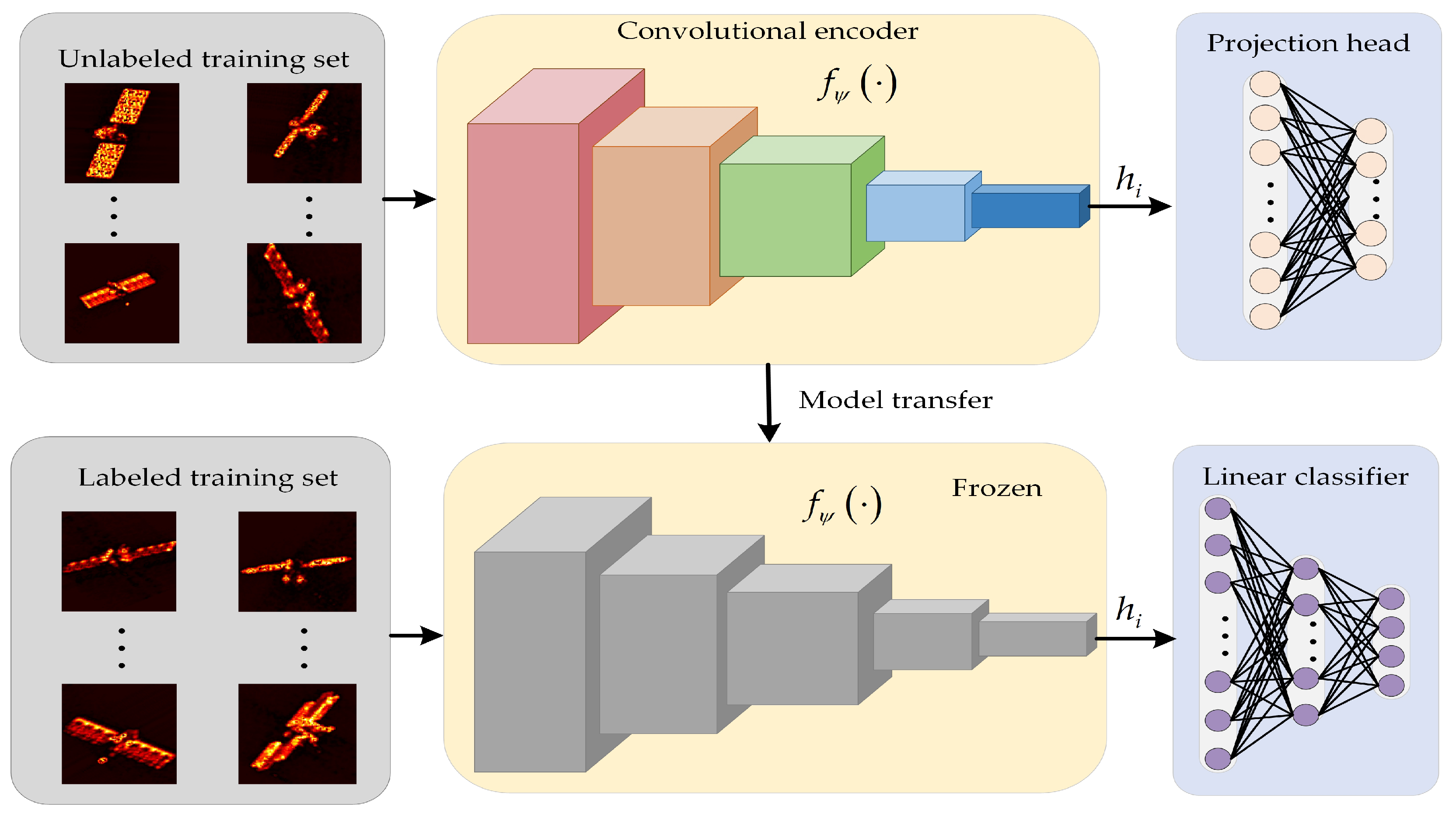
In this section, CLISAR-Net is proposed to obtain the deep representations of deformation ISAR images through unsupervised CL, and then realize ISAR image classification based on the deep representations. This method belongs to unsupervised learning and contains two phases: pretraining and fine-tuning. As shown in Figure 3, the encoder in CLISAR-Net is first pretrained with unlabeled data in the pretraining phase to obtain the deep discriminative representations of the deformation ISAR images. In the fine-tuning phase, to accommodate specific downstream classification tasks, the classifier is fine-tuned with labeled training samples on the basis of the obtained deep representations. Actually, the traditional CNN-based deformation ISAR image classification networks are trained directly from the second phase, and they are all supervised learning methods.

3.1. Unsupervised Pretraining with Unlabeled Data

Compared with the traditional deformation ISAR image classification networks, CLISAR-Net can be pretrained without any manually labeled samples. This is because CL can motivate the encoder to learn higher-level representations by comparing the similarity between amounts of unlabeled samples and empower it to distinguish samples from different categories. In the pretraining phase of CLISAR-Net, the following issues should be considered: the structure of the encoder, loss function of CL, and the optimization of the encoder.

3.1.1. Structure of the Encoder

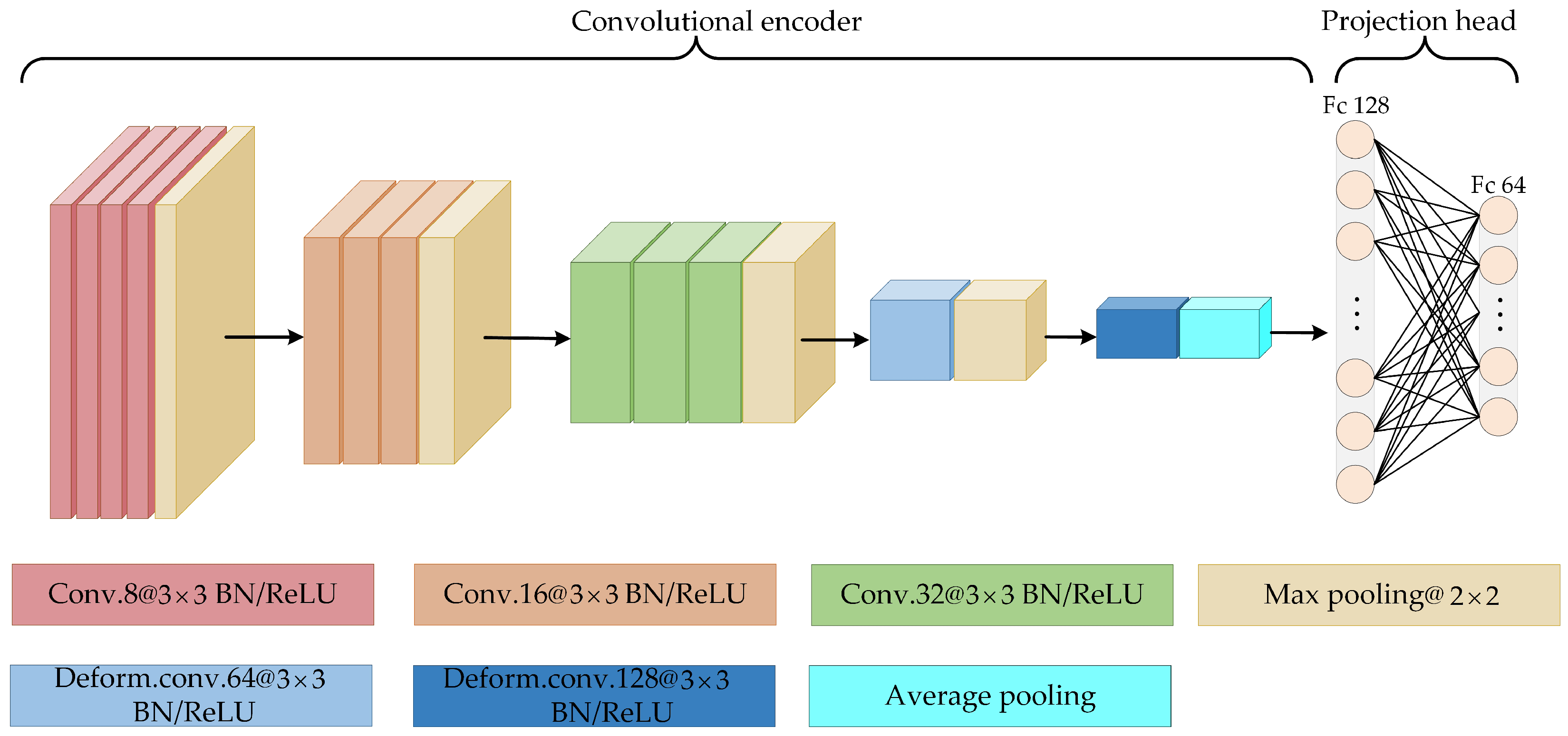
The goal of CL is to learn an encoder that can extract the deep representations of samples. In CLISAR-Net, the encoder contains two parts: the convolutional encoder and the projection head, in which the former is what we hope to obtain through unsupervised pretraining. Figure 4 shows the structure of the encoder. The convolutional encoder is stacked with five convolution-pooling blocks, and regular 2D convolutions are used in the former three blocks to learn simple features of ISAR images, such as textures and edges. The latter two blocks are 2D deformable convolutions, the variable convolution kernel can be more adaptive to the structure variation of the deformation ISAR images.
In the convolutional encoder, Conv.8@ 3 × 3 BN/ReLU indicates that there are eight regular convolution kernels sized 3 × 3 with batch normalization (BN), and ReLU represents rectified linear unit activation. Max pooling@ 2 × 2 indicates a max-pool layer with a kernel size of 2 × 2 and step of 2. For the mth channel of the input feature map I m ( l ) , the nth channel of the output feature map O n ( l + 1 ) is computed as follows:
O n ( l + 1 ) = σ B N m M conv I m ( l ) , K n ( l + 1 ) + b n ( l + 1 )
where K n ( l + 1 ) and b n ( l + 1 ) are the learnable weights and bias of the ( l + 1 ) th layer in the nth channel, and M is the number of channels for the input feature map. The pixel value of the output feature map at ( x , y ) is calculated by:
conv ( I , K ) x , y = p = 0 P 1 q = 0 Q 1 I x p , y q K p , q
where P × Q is the kernel size, and I x p , y q and K p , q denote the pixel values of the input feature map I and the convolution kernel K at ( x p , y q ) and ( p , q ) , respectively. BN for a mini-batch data X is defined as follows:
B N ( X ) = α × X μ B σ B 2 + ε + β
where μ B and σ B 2 are mean and variance of the data, ε is a small value that avoids division by zero, and α , β are learnable parameters. Gradient disappearance and explosion can be alleviated by BN. σ ( · ) is a ReLU non-linear activation function, which can be written as:
σ ( X ) = max ( 0 , X )
Pooling can usually be seen as a downsampling operation. For the mth channel of I m ( l ) , after the max-pooling window with a kernel size of 2 × 2 and step size of 2, the pixel value of the output feature map at ( x , y ) is:
P n ( l + 1 ) = max I m ( l ) ( 2 x + p , 2 y + q ) p = 0 , 1 ; q = 0 , 1
In the convolutional encoder, Deform conv.64@ 3 × 3 BN/ReLU denotes that there are sixty-four deformable convolution kernels sized 3 × 3 , also with BN and a ReLU activation. The deformable convolution adds the learned offset to each sampling position of the receptive field, making the deformable sampling locations able to sample the structural information around the pixel of interest. Additionally, the extracted features are more adaptable to scaling, rotation, and other deformations of ISAR images.
The implementation process of deformable convolution is shown in Figure 5. The offset field is first generated using the offset generator to obtain the offset values, then the input feature maps will be resampled using bilinear interpolation to obtain the deformation feature maps. Finally, the output feature maps are generated by regular 2D convolution on the the deformation feature maps.
The offset generator is a convolution layer with 3 × 3 kernels, and the offset field is obtained by convolution on the input feature maps. For any pixel position ( x , y ) of I R F x × F y ( F x × F y is the size of the input feature map), two offsets x offset and y offset are learned in the offset field, i.e., offsets Δ F = x offset , y offset R 2 M × F x × F y , where 2 M is the number of channels. Since x offset and y offset may be fractional, the new position x new , y new = x + x offset , y + y offset obtained by resampling usually deviates from integer pixels. Therefore, the bilinear interpolation is required to calculate the pixel value at x new , y new in the deformation feature maps from the pixels around ( x , y ) in the input feature maps. Assuming that I x , y is the pixel value at ( x , y ) , the output pixel value I ^ x new , y new is calculated as follows:
I ^ x new , y new = x F x y F y I x , y max 0 , 1 x new x max 0 , 1 y new y
After the above bilinear interpolation to obtain the deformation feature maps, the final output feature maps can be obtained by regular 2D convolution. The whole computation of deformable convolution is summarized as follows:
deform . conv ( I , K , Δ F ) x , y = p = 0 P 1 q = 0 Q 1 I ^ x p + x offet , y q + y offset K p , q
where I ^ denotes the deformation feature maps.
After Deform conv.128@ 3 × 3 BN/ReLU, the obtained output feature maps are converted into feature vectors using average pooling. For an input ISAR image sample x i , the feature vector representation obtained by the above convolutional encoder f ψ ( · ) is denoted as h i = f ψ x i , where ψ denotes all the learnable parameters. Then, the feature vector representation is mapped into the feature space by a projection head g ξ ( · ) , where ξ is the learnable parameters of g ξ ( · ) . In this article, the projection head is constructed by two fully connected layers. For the input x i , the vector representation output by the projection head is:
q i = g ξ h i = W ( 2 ) σ W ( 1 ) f ψ x i + b ( 1 ) + b ( 2 )
where W , b ξ indicate the learnable parameters of the projection head. Recent work has shown that calculating the contrastive loss on q i is more efficient than h i [38]. The above convolutional encoder f ψ ( · ) and projection head g ξ ( · ) constitute the base encoder f q ( · ) for extracting the deep representations from input ISAR image samples. The loss function of CL is elaborated below.

3.1.2. Loss Function of CL

Traditional supervised learning methods are based on category discrimination, which need to provide the category information manually. CL is a pretext task based on instance discrimination, that is, each sample is regarded as a category, so the samples themselves provide supervised information, and no manual annotation is required. Therefore, the cross-entropy loss function commonly utilized in category discrimination is no longer suitable for instance discrimination, and it is necessary to be modified.
Consider a training set X = { x 1 , x 2 , , x Z } R d × Z , where x i denotes the ith training sample and d is the dimension of the data. Another view of the training set X can be written as X ˜ = { x ˜ 1 , x ˜ 2 , , x ˜ Z } R d × Z , where x i and x ˜ i are different views of the same sample, and they are treated as a positive sample pair, while x i and x ˜ j ( j = 1 , 2 , , Z , j i ) form Z 1 negative sample pairs. To facilitate the distinction, we denote x ˜ i as x i + and x ˜ j as x j . For a sample x i , it is encoded as q i = f q x i , and similarly, x i + and x j are encoded as q i + = f q ˜ x i + and q j = f q ˜ x j , respectively, where f q ( · ) is the base encoder that needs to be pretrained, and f q ˜ ( · ) is the auxiliary momentum encoder that is necessary for pretraining f q ( · ) . The contrastive loss needs to realize the following relationship:
sim q i , q i + sim q i , q j
where sim ( · , · ) is a function that measures the similarity of two samples. In CL, the InfoNCE loss function is often used to implement the above relationship. The InfoNCE loss of the deep representation q i is defined as follows:
L q i , q i + , q j = log exp sim q i , q i + / τ exp sim q i , q i + / τ + q j exp sim q i , q j / τ
where τ is a temperature hyperparameter. In the above equation, the number of negative sample pairs is Z 1 , which means the upper limit of j is Z 1 . As described in the definition, this loss function is a Z-way log loss based on softmax classifier, which tries to classify q i as q i + [49]. In this article, the vector dot product is utilized to measure the similarity of two samples, i.e.,
sim q i , q i + = q i T q i + , sim q i , q j = q i T q j
In the InfoNCE loss, each q i + is a positive sample of q i and also participates in the calculation of InfoNCE loss as a negative sample of all q j ( j i ) . Actually, a positive sample pair in CL provides supervision to each other.

3.1.3. Optimization of the Encoder

As mentioned above, an auxiliary momentum encoder is also needed for pretraining the base encoder. As shown in Figure 6, the momentum encoder and the base encoder form a parallel dual-stream architecture, and they share the same network structure and hyperparameters [50]. For an ISAR image sample x i , the data-augmented view of it is x i + , they form a positive pair. Similar to Equation (10), x i + is fed into the momentum encoder to obtain its deep representation:
q i + = g ξ ˜ f ψ ˜ x i +
where f ψ ˜ ( · ) and g ξ ˜ ( · ) are the convolutional encoder and projection head of the momentum encoder. Based on the above description, the positive pair, i.e., q i and q i + , can be produced by the two encoders, respectively, and they are both vectors with dimensions of C.
CL requires an amount of negative pairs when calculating InfoNCE loss; this is because a rich set of negative samples allows the encoder to learn features that are more conducive for discrimination [42]. Consider a mini-batch with N training samples, when CLISAR-Net is optimized by gradient descent on a mini-batch, the number of negative pairs is N 1 . To satisfy the InfoNCE loss calculation, a large mini-batch size is needed, but increasing the mini-batch size will bring some adverse effects. For example, as the mini-batch size increases, more memory space is needed, but most standard computing platforms struggle to support such requirements. At the same time, a large mini-batch size will reduce the optimization efficiency. Inspired by previous works [39,42], this article introduces a memory bank to store the negative samples. As shown in Figure 6, the encoded representations of the momentum encoder in the previous mini-batches are stored in the memory bank in turn. In order to utilize more negative pairs, the encoded representations of the momentum encoder in the current mini-batch are not used as negative samples in the InfoNCE loss calculation but are provided by the memory bank. That is, in the current mini-batch, the positive samples are provided by the momentum encoder, while the negative samples come from the memory bank. By calculating the InfoNCE loss, the base encoder can be updated through backpropagation.
During the pretraining of CLISAR-Net, the encoded representations q + of the momentum encoder in each mini-batch are stored into the memory bank in turn. Since the samples in each mini-batch have no intersection, for the output representations q of the current mini-batch, the q + of all the previous mini-batches can be viewed as negative samples of q . This means that output representations of the momentum encoder for the previous mini-batches can be reused. Supposing that the length of the memory bank is K, then K = k × N . The introduction of the memory bank expands the number of available negative samples, so the number of negative sample pairs is equal to the length of the memory bank and no longer depends on the mini-batch size. Such a design provides more negative sample pairs for the InfoNCE loss calculation and ensures the effectiveness of CL. Moreover, traversing negative samples from the memory bank does not require additional computations, which provides a guarantee for efficient training of CLISAR-Net.
It should be pointed out that the negative samples in the memory bank vary dynamically. In CLISAR-Net, the memory bank is maintained as a queue of negative samples, and the encoded representations output by the momentum encoder will be enqueued into the memory bank after each mini-batch training is completed. When the new representations cannot be enqueued into the memory bank, the representations of the oldest mini-batch will be dequeued from the memory bank, and the new output of the current mini-batch will be enqueued, thereby updating the negative samples dynamically. As the momentum encoder is continuously optimized, and the output encoded representations are gradually updated, the representations of the oldest mini-batch are the most outdated and the most inconsistent with the newest ones. Therefore, in order to maintain the consistency of negative samples, it is necessary to maintain a slowly updated memory bank. In addition, a slowly and dynamically updated memory bank requires less memory space and is more beneficial to maintain the consistency of negative samples than storing the representations of all samples in the dataset [42].
The utilization of the memory bank makes it difficult to update the momentum encoder by loss backpropagation, so the optimization of the momentum encoder needs to be adjusted accordingly. The momentum encoder in CLISAR-Net provides negative samples that support InfoNCE loss calculation, and the negative samples play a partially supervisory role during training, so there should not be too much difference between them. That is, the update of the momentum encoder should be smooth. In this article, we use a momentum update to optimize the momentum encoder, namely:
ψ ˜ m ψ ˜ + ( 1 m ) ψ , ξ ˜ m ξ ˜ + ( 1 m ) ξ
where m [ 0 , 1 ) is a momentum coefficient, which is the meaning of the word momentum. It shows that only the parameters ψ and ξ of the base encoder are updated by InfoNCE loss backpropagation. The momentum update in Equation (15) makes the parameters ψ ˜ and ξ ˜ evolve more smoothly than ψ and ξ . Therefore, although the negative samples in the memory bank are generated by different momentum encoders, the differences between them are small. The experimental results in [39] prove that a larger momentum coefficient will make the momentum encoder update more smoothly, which is also more beneficial to maintain the consistency of negative samples.

3.2. Classifier Fine-Tuning with Labeled Data

The deep representations of deformation ISAR images obtained by pretraining in Section 3.1 cannot be directly used for classification. Therefore, in this section, the pretrained convolutional encoder is transferred to the downstream supervised learning, and a linear classifier is fine-tuned using labeled samples. The diagram of classifier fine-tuning in CLISAR-Net is shown in Figure 7. Specifically, throw away the projection head of the pretrained base encoder, and only the convolutional encoder is retained. In the fine-tuning process, the convolutional encoder is frozen and is directly used to extract the deep representations of labeled training samples. In the fine-tuning phase, only the lightweight classifier will be trained, and the convolutional encoder is not involved. Due to the low complexity of the linear classifier, a small number of labeled samples are sufficient for training.

4. Experiments

4.1. Data Generation

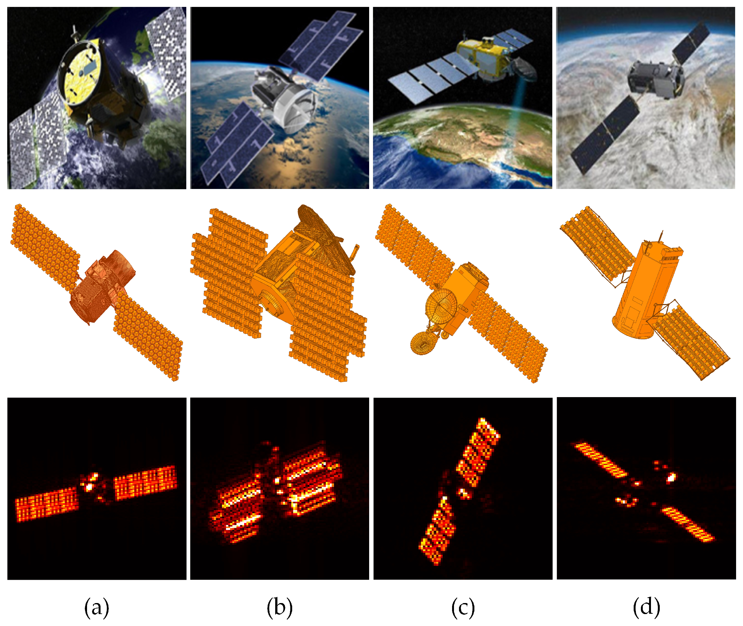
To verify the unsupervised deep representation learning ability of the proposed CLISAR-Net for deformation ISAR images and the classification ability using labeled samples, we conduct experiments on a high-resolution ISAR image dataset including four satellites, i.e., CALIPSO, Cloudsat, Jason-3, and OCO-2 [51]. In experiments, echoes of the target are generated using the shooting and bouncing ray (SBR+) method in the HFSS 2021R2 software developed by Ansoft in the United States.
In the EM calculation, we set radar works in the central frequency of 17 GHz with HV polarization, the imaging bandwidths are 1 GHz (16∼17 GHz), 1.5 GHz (16∼17.5 GHz), and 2 GHz (16∼18 GHz). The azimuth angle γ is 0 ∼359 with an interval of 0 . 05 . The accumulating angle Δ θ is set to 4 , 5 , and 6 , respectively. Meanwhile, in order to verify the classification performance of CLISAR-Net for satellite targets at different elevation angles, we set two elevation angles for four satellites, respectively, i.e., φ 1 = 55 and φ 2 = 60 for CALIPSO, φ 1 = 50 and φ 2 = 55 for Cloudsat and Jason-3, and φ 1 = 65 and φ 2 = 70 for OCO-2. The RD algorithm is used to perform continuous high-resolution ISAR imaging. For the convenience of classification, each ISAR image is cropped to 128 × 128 pixels. The optical images, CAD models, and typical ISAR images of CALIPSO, Cloudsat, Jason-3, and OCO-2 are shown in Figure 8.
As stated in Section 2, different radar parameters will cause scaling deformation of ISAR images; meanwhile, the target motion will cause rotation deformation of ISAR images. In practice, scaling and rotation deformations usually occur simultaneously during observation, resulting in complex deformation of ISAR images. Therefore, in the experiments, three datasets are generated, namely scaled, rotated, and combined deformation datasets, to evaluate the performance of CLISAR-Net on ISAR images with different deformations. The details of these three datasets are described below.

4.1.1. Scaled Deformation Dataset

To evaluate the classification ability of CLISAR-Net for scaled deformation ISAR images due to range and azimuth scaling, a scaled deformation dataset is generated, as shown in Table 1. The elevation angles of the four satellites in the training and test sets are all φ 1 . The other imaging parameters are Δ θ = 5 , B = 1 GHz and Δ θ = 6 , B = 2 GHz for the training set, while becoming Δ θ = 6 , B = 1.5 GHz and Δ θ = 4 , B = 2 GHz for the test set. The above parameter settings cause the training and test ISAR images to be scaled along both the range and azimuth dimensions. In the scaled deformation dataset, the training sets have 2836 samples, and the test sets have 2840 samples.

4.1.2. Rotated Deformation Dataset

The rotated deformation ISAR image dataset is shown in Table 2. The same bandwidths and accumulating angles are used in the training and test sets, i.e., Δ θ = 5 , B = 1 GHz and Δ θ = 6 , B = 2 GHz. However, the elevation angles of the four satellites in the training set are all φ 1 , and in the test set are all φ 2 . Furthermore, a quarter of the azimuth angles are lost in the training set, i.e., the azimuth angle γ is 90 ∼359 . Such a setting can verify the ability of CLISAR-Net to extract discriminative representations of the rotated deformation ISAR images when the training samples do not cover all the observation intervals. In the rotated deformation dataset, there are 2116 samples in the training set and 2836 samples in the test set.

4.1.3. Combined Deformation Dataset

In practical observations, ISAR images usually exhibit a combined deformation of scaling and rotation. To analyze the classification robustness of CLISAR-Net in this scenario, a combined deformation ISAR image dataset is constructed, and the parameter settings are shown in Table 3. The elevation angle in the training set is φ 1 , while changing to φ 2 in the test set. The other parameters are Δ θ = 5 , B = 1 GHz and Δ θ = 6 , B = 2 GHz for the training set, while they are Δ θ = 6 , B = 1.5 GHz and Δ θ = 4 , B = 2 GHz for the test set. The combined deformation dataset includes both scaling and rotation deformations, so this group of ISAR images has the most obvious deformations. Same as the rotated dataset, 1/4 of azimuth angles are lost in the training set for the combined dataset, which increases the difficulty of classification. In the combined deformation dataset, there are 2116 training samples and 2840 test samples.

4.2. Experimental Setup

4.2.1. Data Augmentations

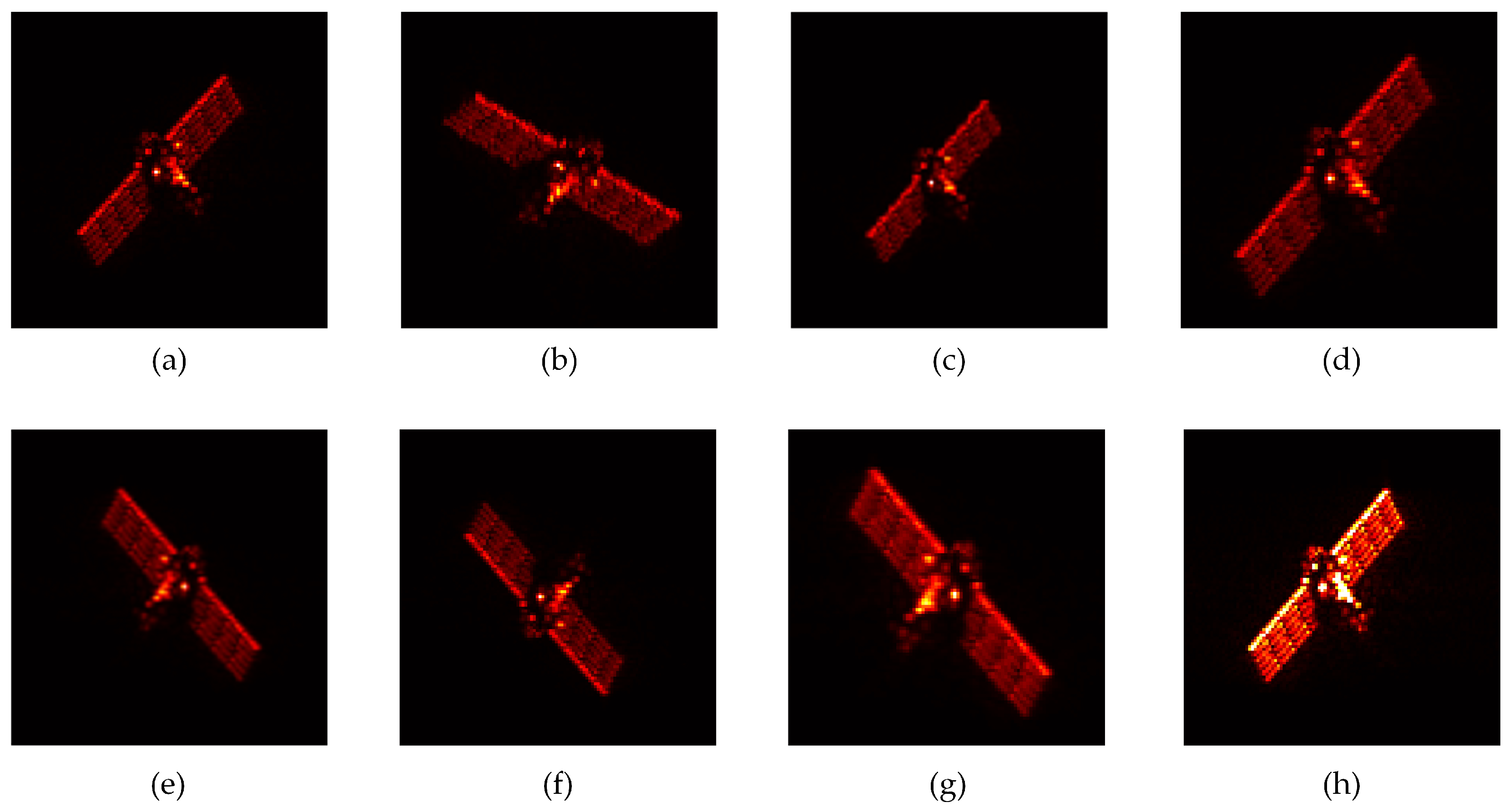
The data augmentations employed in the training of CLISAR-Net include: (i) random rotation and scaling for the ISAR images with the probability of 0.5, where the rotation angles are uniformly distributed in ± 90 , and the scaling ratio is uniformly distributed in ± 0.2 ; (ii) random horizontal or vertical flips for the ISAR images with the probability of 0.5; (iii) random center cropping (by 0.8 × 1.2 × ) for the ISAR images and resizing them to 128 × 128 pixels; and (iv) performing ISAR images amplitude normalization to eliminate the effect of amplitude. The above data augmentations provide more deformation patterns and enable the pretrained base encoder of CLISAR-Net to learn more deformation information. Figure 9 visualizes the data augmentations that we use in this work. During pretraining, two independent data augmentation operators are randomly generated from the above augmentations and applied to each training sample x i to obtain two different views, and then they are fed into the base encoder and momentum encoder, respectively. Since deep representations of deformation ISAR images were obtained by pretraining, only the normalization operator is used for data normalization in classifier fine-tuning.

4.2.2. Parameter Settings

In the pretraining phase, the structure of the convolutional encoder is shown in Figure 4. The convolutional kernels are all sized 3 × 3 with a step size of 1 × 1 . The max pooling layers are all sized 2 × 2 with a step size of 2. The kernel numbers in five convolution-pooling blocks are 8, 16, 32, 64, and 128, respectively. For the projection head, the nodes of the two fully connected layers are 128 and 64. The momentum encoder has exactly the same structure as the base encoder, which is very important to maintain consistency. For the pretraining, the CosineAnnealing learning rate schedule is used with a maximum learning rate of 0.001 and a half-period of 50 epochs. The mini-batch size is 256, and the Adam optimizer is used to train for 500 epochs. Meanwhile, the momentum coefficient m = 0.999 , the length of the memory bank is 8192, and the temperature τ = 0.1 . The pretraining is implemented by two NVIDIA RTX3090 GPUs using distributed training.
In the fine-tuning phase, the linear classifier connected behind the average pooling layer contains two fully connected layers with 64 and 32 nodes, and the nodes of the softmax layer are 4. The OneCycle learning rate schedule is used to train the linear classifier. Based on the Adam optimization, the classifier is trained for 200 epochs with a maximum learning rate of 0.001. The mini-batch size is 32. The retraining and the testing process are both performed by one NVIDIA RTX3090 GPU. The entire CLISAR-Net is implemented by Pytorch on Ubuntu20.04 Linux system.

4.2.3. Comparison Methods

In order to verify the ability of CLISAR-Net for deformation ISAR image classification, four supervised and a semi-supervised classifiers are compared in the experiments. Specifically, four CNN-based supervised models are chosen, including CNN, spatial transformer–convolutional neural network (ST-CNN) with a double layer of STN [31], Deform-CNN using the deformable convolutional network (DCN) [32], and CNN connected to BiLSTM (CNN-BiLSTM) [52]. Moreover, the support vector machine (SVM) is chosen as a semi-supervised model. Among them, CNN has the same structure as the convolutional encoder described in Section 3.1.1, except that the deformable convolution in the last two blocks is replaced by regular convolution. The ST-CNN shares the same convolution kernels with CNN, but it adds a double layer of STN before CNN. The structure of Deform-CNN is identical to the convolutional encoder described in Section 3.1.1. It must be pointed out that the Deform-CNN here is trained in a supervised paradigm. A double layer of BiLSTM connected behind CNN constitutes the CNN-BiLSTM, which can be used to process the sequential ISAR images. The input sequential ISAR images of CNN-BiLSTM can be obtained by a continuous sliding window [52]. In the experiments, the length of the sliding window is set to 10, and the step size is 1.
Based on the Adam optimization, the parameter updates of the above networks are all achieved by cross-entropy loss backpropagation. Similarly, these supervised networks for comparison are trained using the CosineAnnealing learning rate schedule with a half-period of 25 epochs. The maximum learning rate is 0.001 for all the networks except ST-CNN, which has a learning rate of 0.0001. This is because STN is sensitive to the learning rate, and a smaller learning rate is helpful for STN to train the ISAR images. The mini-batch size is set to 32, and 200 epochs are trained.

4.3. Classification Results

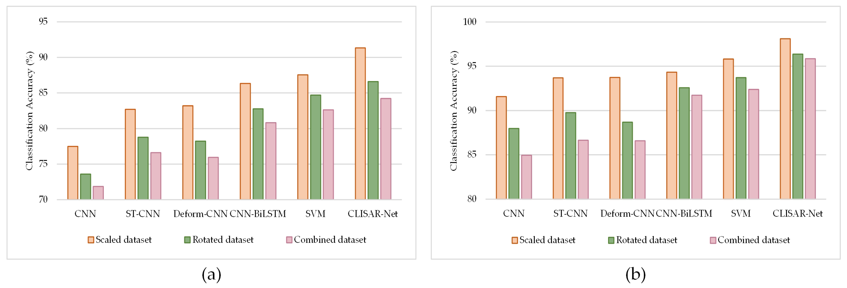
In the experiment, all the unlabeled training samples are used to pretrain the convolutional encoder in CLISAR-Net to obtain the deep representations of ISAR images. Then, based on the learned representations, the linear classifier in CLISAR-Net is fine-tuned using 5% and 100% of the labeled training samples, respectively, to evaluate the classification ability of CLISAR-Net for deformation ISAR images. Table 4 presents the classification results on the three datasets. We can see that the proposed CLISAR-Net achieves the best classification accuracy under the above conditions. The increase in the number of labeled samples provides more supervised information for training, so better performance is obtained when 100% of labeled samples are used.
When only 5% of labeled samples, i.e., 35 samples per category in the scaled dataset and 26 samples per category in the rotated and combined dataset, are used to train the classifiers, CNN has the lowest classification accuracy because there are no mechanisms to deal with ISAR image deformation. The STN network in ST-CNN can adjust the input deformation ISAR image to the view that is easier to recognize. Therefore, the classification accuracy of ST-CNN on the three datasets is improved by 5.21%, 5.18%, and 4.75% over CNN, respectively. Deform-CNN is more adaptable to the deformations of ISAR images through deformable convolution, so it obtains comparable classification ability with ST-CNN. CNN-BiLSTM achieves bidirectional feature extraction and fusion for sequential ISAR images and extracts more deformation-robust features than a single image, thus achieving the best performance among the four supervised models. The classification accuracy of CNN-BiLSTM is 8.84%, 9.19%, and 8.95% higher than CNN on the three datasets. Based on the deep feature representations of deformation ISAR images obtained by CLISAR-Net in the unsupervised pretraining phase, SVM achieves slightly higher classification performance than the other four supervised learning methods. However, the proposed CLISAR-Net achieves the best classification performance. The classification accuracy of CLISAR-Net on the scaled, rotated, and combined deformation datasets reaches 91.34%, 86.61%, and 84.23%, respectively.
When the classifiers are trained using 100% of labeled training samples, the classification accuracy of CLISAR-Net reaches 98.10% for the scaled dataset, 96.37% for the rotated dataset, and 95.85% for the combined deformation dataset. It outperforms the best performing supervised model CNN-BiLSTM by 3.77%, 3.79%, and 4.12%, respectively. Based on the deep representations obtained by unsupervised pretraining, the SVM classifier also performs slightly better than the other four supervised methods. It indicates that in the pretraining phase, based on instance discrimination, CL makes the encoder learn deep discriminative representations of deformation ISAR images, which provides a great help to the classification.
To facilitate the analysis, Figure 10 gives the histograms of the classification results when using 5% and 100% of labeled samples to train the above classifiers. We can summarize that the classification accuracy is the highest for the scaled deformation dataset and the lowest for the combined deformation dataset. Particularly, the classification accuracy for CNN, ST-CNN, and Deform-CNN shows a significant decrease on the rotated and combined deformation datasets. It implies that the traditional end-to-end model for classification based on a single image is difficult to learn deformation-robust features of complex deformation ISAR images when part of the training samples are missing continuously. Comparatively, CNN-BiLSTM maintains a relatively high classification performance on the rotated and combined deformation datasets by fusing the information of multiframe ISAR images. When 100% of the labeled training samples are used to fine-tune the classifier, SVM and CLISAR-Net are less affected by sample misses, especially CLISAR-Net, which shows a more balanced classification performance on the three datasets. Furthermore, from Figure 10a, the classification accuracy of CLISAR-Net exceeds 90% for the scaled deformation dataset, with only 5% of labeled samples, while the CNN is less than 80%. It can be concluded that the smaller the number of labeled training samples, the more obvious the superiority of CLISAR-Net.

4.4. Computational Cost

In this subsection, the computational cost of the proposed CLISAR-Net versus other methods is analyzed, including the computational complexity and the inference time, i.e., the average period for acquiring a frame of an image label in the test process. We measure the computational complexity of the model in terms of the number of trainable parameters. As shown in Table 5, the ST-CNN has the largest number of parameters and the longest inference time due to the addition of a double layer of STN. The number of parameters in Deform-CNN is slightly higher than that in CNN because 2D offsets need to be calculated. The double layer of BiLSTM in CNN-BiLSTM similarly brings an additional number of parameters to the model. The SVM itself has no parameters to be retrained, so the inference time is the shortest. For CLISAR-Net, the pretrained encoder adopts the same structure as Deform-CNN, and only the linear classifier needs to be retrained in the downstream classifier, so the number of trainable parameters is medium. Moreover, the average inference time for obtaining a frame of an image label is only 0.1125 ms. The above analysis shows that CLISAR-Net can achieve the optimal classification performance with less computational cost, which also proves the superiority of CLISAR-Net.

5. Discussion

To demonstrate the superiority of CLISAR-Net for deformation ISAR image classification, Section 5.1 discusses the classification results when different numbers of labeled training samples are used to train the classifiers. Section 5.2 discusses the classification performance of CLISAR-Net when different azimuth angle ranges are included in the training set. Additionally, the features learned by the CLISAR-Net and CNN-BiLSTM are visualized in Section 5.3.

5.1. Effect of Different Training Ratios

To evaluate the effect of a different number of labeled training samples on the deformation ISAR image classification, CNN, ST-CNN, Deform-CNN, CNN-BiLSTM, SVM, and the proposed CLISAR-Net are tested using different ratios of labeled training samples. Figure 11 reports the comparison results on the scaled, rotated, and combined deformation datasets. It can be seen from the results of the three datasets that CLISAR-Net performs the best in all conditions, followed by SVM. Moreover, the classification accuracy increases gradually with the increase in the number of labeled samples, which is consistent with the expectation. When only 5% of labeled samples are used to train CLISAR-Net, the CNN requires 100% of labeled samples to achieve similar classification performance for the three datasets. The performance of ST-CNN and Deform-CNN is always very close, but ST-CNN is more difficult to train. The results of the scaled dataset exemplify the superiority of CLISAR-Net at the ratios of 5%, 10%, and 20%. For the combined dataset, as shown in Figure 11c, when 20% of labeled samples are used, the classification accuracy of CLISAR-Net has a greater improvement than SVM and CNN-BiLSTM. Based on the above analysis, it is reasonable to assume that discriminative deep representations were learned in the unsupervised pretraining phase. As a result, CLISAR-Net can achieve good performance by fine-tuning the classifier with only a small number of labeled samples.

5.2. Extended to Different Azimuth Angle Ranges

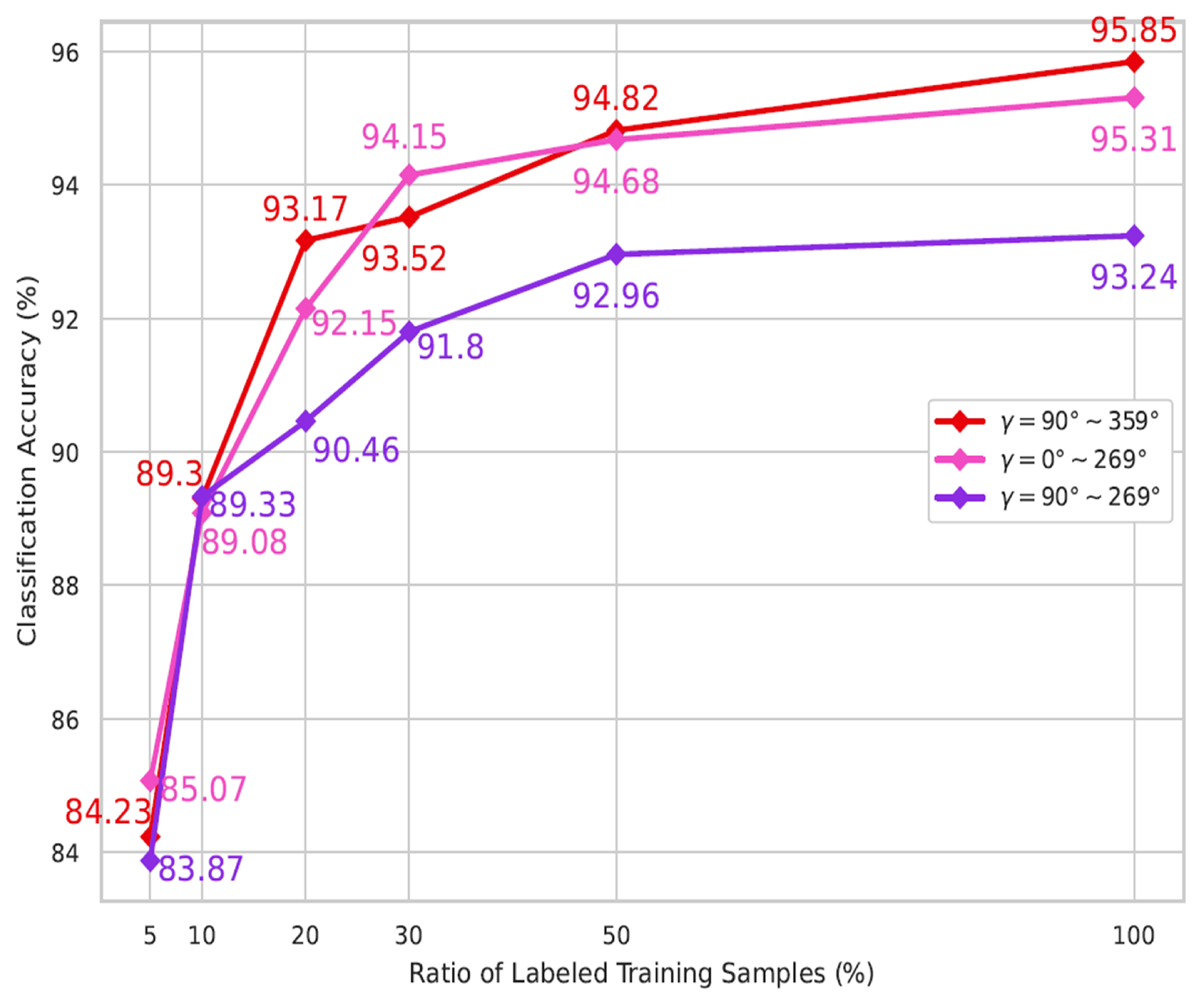
To evaluate the classification robustness of CLISAR-Net for the deformation ISAR images when different azimuth angles are missing in the training set, the azimuth angle γ in the training set of the combined deformation dataset is adjusted to 0 269 and 90 269 , while the test set is kept constant. In the adjusted combined deformation dataset, the numbers of samples in the training sets are 2116 and 1396, respectively, and the number of samples in the test set is still 2840. Figure 12 shows the classification results of CLISAR-Net for the test set when the ranges of the azimuth angle in the training set are γ = 90 359 , γ = 0 269 , and γ = 90 269 . As can be seen in Figure 12, the two polylines corresponding to γ = 90 359 and γ = 0 269 are intertwined, which indicates that CLISAR-Net has robust classification performance when 1/4 of the azimuth angles are missing in the training set. For the azimuth angle ranges from 90 to 269 , the classification accuracy of CLISAR-Net reaches 93.24% after fine-tuning the downstream classifier using 100% of the labeled training samples, which is only 2.61% and 2.07% lower than that when 1/4 of the azimuth angles are missing, respectively. However, it is not difficult to find that when only 5% and 10% labeled training samples are used to fine-tune the downstream classifier, high classification performance is achieved, even though 1/2 of the azimuth angles are missing in the training set. This reaffirms the conclusion that CLISAR-Net can achieve superior classification accuracy when only a small amount of labeled data are available.

5.3. Visualization of Features

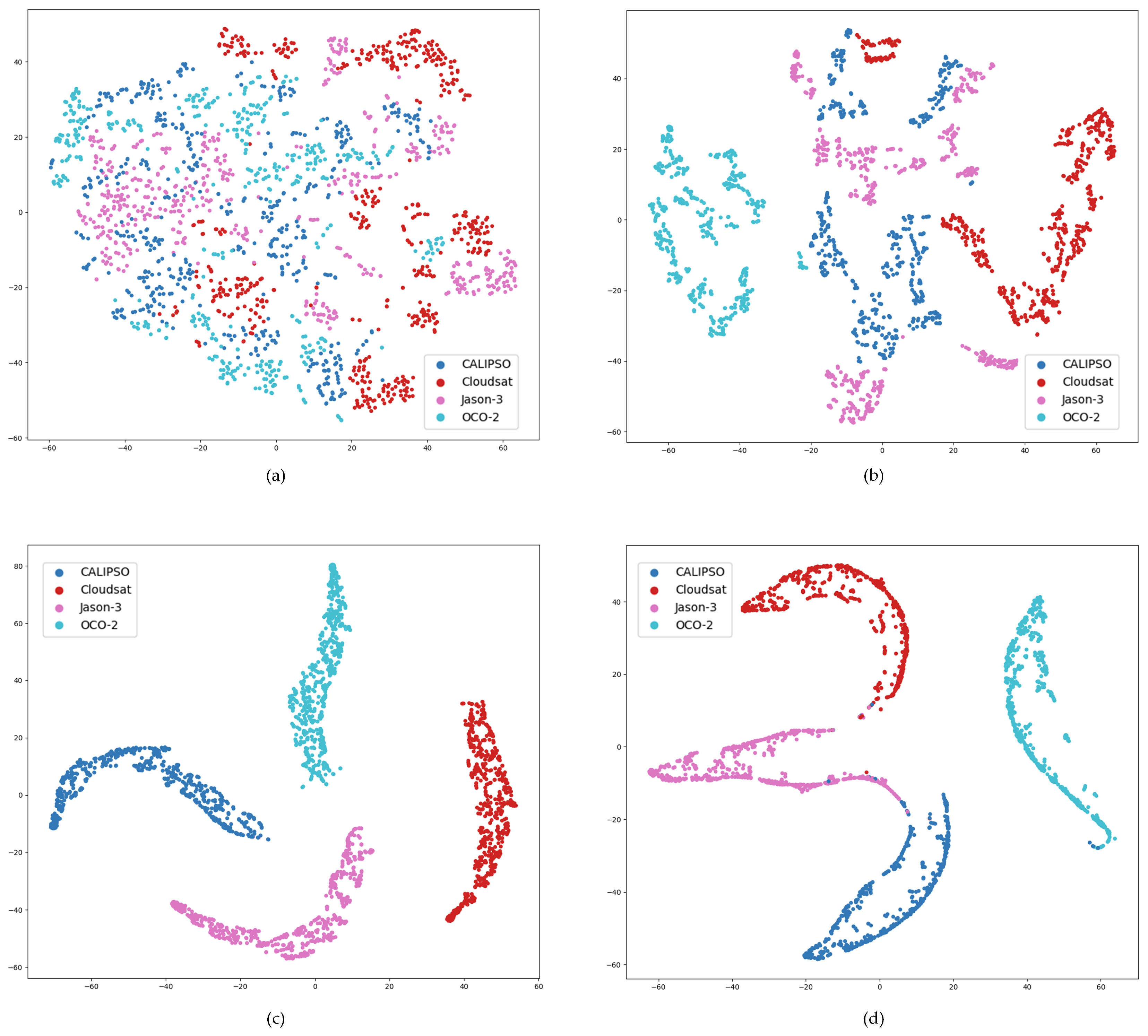
The CLISAR-Net performs well on the three datasets, and the essential reason is that the convolutional encoder can extract the deep representations of unlabeled ISAR images during pretraining. To explicitly view the extracted representations, 2D visualizations of the feature representations are performed by t-SNE [53] for the combined deformation dataset. As shown in Figure 13, the distance of points indicates the similarity between samples. Samples of the same satellite are represented by points of the same color, where dark blue points denote CALIPSO, red points indicate Cloudsat, pink points are Jason-3, and cyan points are OCO-2.
The features learned by CLISAR-Net in different training phases and the features learned by CNN-BiLSTM, the best performing classification model in the supervised methods, are visualized by t-SNE. In Figure 13, each point represents an ISAR image. From the distribution of the input images, it can be seen that in the combined deformation dataset, the points of different categories are widely distributed in different positions and are completely indistinguishable. Figure 13b shows the distribution of the deep representations obtained by unsupervised pretraining. Compared with Figure 13a, the compactness within each category is increased significantly. OCO-2 is basically separable, and most of the points of the other three categories are separable. The visualization results show that unsupervised pretraining can embed the features of the input images into a more discriminative space. In Figure 13c, the linear classifier in CLISAR-Net is fine-tuned to create more compact category clusters based on Figure 13b and achieves better feature separation for the four satellites. In Figure 13d, although the CNN-BiLSTM improved the feature separability of the four categories, the feature distribution of CALIPSO and Jason-3 still has partial overlap and coverage, so its classification performance is slightly inferior to that of CLISAR-Net, which agrees with the classification results in Table 4.

6. Conclusions

In order to achieve deformation ISAR image classification, an unsupervised ISAR image deep representation learning method is explored based on CL for the first time. The training of CLISAR-Net consists of two phases, i.e., unsupervised pretraining and classifier fine-tuning. In the pretraining phase, the base encoder is optimized by InfoNCE loss backpropagation, and the evolution of the momentum encoder is realized by the momentum update of the parameters. With the help of the discriminative representations obtained by pretraining, high-precision classification of deformation ISAR images can be achieved by retaining the convolutional encoder and fine-tuning the linear classifier. CLISAR-Net demonstrates powerful classification performance in the experiments on scaled, rotated, and combined deformation ISAR image datasets. Compared with traditional CNN-based supervised learning methods, the added unsupervised pretraining phase in CLISAR-Net makes the feature extractor capture more discriminative deep representations of deformation ISAR images, which brings great convenience for downstream classification and enables CLISAR-Net to achieve higher classification performance with a small number of labeled samples.
Although the proposed CLISAR-Net requires two phases to achieve classification, the encoder structure that extracts the feature of deformation ISAR images is simpler than that of the CNN-based methods. Moreover, based on CL, CLISAR-Net opens the door for researches of ISAR image classification based on unsupervised learning. In the future, ISAR image classification will be performed by combining the EM scattering mechanism and semantic information of the target under unsupervised conditions.

Author Contributions

Conceptualization, G.X. and P.N.; methodology, P.N., Y.L. and H.P.; software, P.N., H.P. and H.D.; validation, P.N. and G.X.; investigation, P.N. and Y.L.; resources, Y.L. and H.L.; data curation, P.N.; writing—original draft, P.N. and H.D.; writing—review and editing, P.N. and G.X.; supervision, G.X. All authors have read and agreed to the published version of the manuscript.

Funding

This work was supported by the National Science Foundation of China (NSFC) under Grant 62071113, in part by the Natural Science Foundation of Jiangsu Province under Grant BK20211559.

Conflicts of Interest

The authors declare no conflict of interest.

References

  1. Kim, K.T.; Seo, D.K.; Kim, H.T. Efficient Classification of ISAR images. IEEE Trans. Antennas Propag. 2005, 53, 1611–1621. [Google Scholar]
  2. Liu, L.; Zhou, F.; Bai, X.; Tao, M.; Zhang, Z. Joint Cross-Range Scaling and 3D Geometry Reconstruction of ISAR Targets Based on Factorization Method. IEEE Trans. Image Process. 2016, 25, 1740–1750. [Google Scholar] [CrossRef]
  3. Wagner, S.; Dommermuth, F.; Ender, J. Detection of Jet Engines via Sparse Decomposition of ISAR Images for Target Classification Purposes. In Proceedings of the 2016 European Radar Conference (EuRAD), London, UK, 5–7 October 2016; pp. 77–80. [Google Scholar]
  4. Huang, Y.; Liao, G.; Xiang, Y.; Zhang, L.; Li, J.; Nehorai, A. Low-rank Approximation via Generalized Reweighted Iterative Nuclear and Frobenius Norms. IEEE Trans. Image Process. 2020, 29, 2244–2257. [Google Scholar] [CrossRef]
  5. Du, Y.; Jiang, Y.; Wang, Y.; Zhou, W.; Liu, Z. ISAR Imaging for Low-Earth-Orbit Target Based on Coherent Integrated Smoothed Generalized Cubic Phase Function. IEEE Trans. Geosci. Remote Sens. 2019, 58, 1205–1220. [Google Scholar] [CrossRef]
  6. Xue, B.; Tong, N. Real-World ISAR Object Recognition Using Deep Multimodal Relation Learning. IEEE Trans. Cybern. 2019, 50, 4256–4267. [Google Scholar] [CrossRef] [PubMed]
  7. Zhang, Y.; Yuan, H.; Li, H.; Chen, J.; Niu, M. Meta-Learner-Based Stacking Network on Space Target Recognition for ISAR Images. IEEE J. Sel. Top. Appl. Earth Obs. Remote Sens. 2021, 14, 12132–12148. [Google Scholar] [CrossRef]
  8. Lee, S.J.; Park, S.H.; Kim, K.T. Improved Classification Performance Using ISAR Images and Trace Transform. IEEE Trans. Aerosp. Electron. Syst. 2017, 53, 950–965. [Google Scholar] [CrossRef]
  9. Benedek, C.; Martorella, M. Moving Target Analysis in ISAR Image Sequences With a Multiframe Marked Point Process Model. IEEE Trans. Geosci. Remote Sens. 2013, 52, 2234–2246. [Google Scholar] [CrossRef]
  10. Islam, M.T.; Siddique, B.N.K.; Rahman, S.; Jabid, T. Image Recognition with Deep Learning. In Proceedings of the 2018 International Cnference on Intelligent Informatics and Biomedical Sciences (ICIIBMS), Bangkok, Thailand, 21–24 October 2018; pp. 106–110. [Google Scholar]
  11. Karine, A.; Toumi, A.; Khenchaf, A.; El Hassouni, M. Radar Target Recognition Using Salient Keypoint Descriptors and Multitask Sparse Representation. Remote Sens. 2018, 10, 843. [Google Scholar] [CrossRef] [Green Version]
  12. Bai, Q.; Gao, G.; Zhang, X.; Yao, L.; Zhang, C. LSDNet: Light-weight CNN Model Driven by PNF for PolSAR Image Ship Detection. IEEE J. Miniat. Air Space Syst. 2022, 3, 135–142. [Google Scholar] [CrossRef]
  13. Gao, S.; Liu, H. RetinaNet-based Compact Polarization SAR Ship Detection. IEEE J. Miniat. Air Space Syst. 2022, 3, 146–152. [Google Scholar] [CrossRef]
  14. Zhang, L.; Gao, G.; Duan, D.; Zhang, X.; Yao, L.; Liu, J. A Novel Detector for Adaptive Detection of Weak and Small Ships in Compact Polarimetric SAR. IEEE J. Miniat. Air Space Syst. 2022, 3, 153–160. [Google Scholar] [CrossRef]
  15. Sun, Y.; Wang, Y.; Liu, H.; Wang, N.; Wang, J. SAR Target Recognition with Limited Training Data Based on Angular Rotation Generative Network. IEEE Geosci. Remote Sens. Lett. 2019, 17, 1928–1932. [Google Scholar] [CrossRef]
  16. Wang, L.; Bai, X.; Gong, C.; Zhou, F. Hybrid Inference Network for Few-Shot SAR Automatic Target Recognition. IEEE Trans. Geosci. Remote Sens. 2021, 59, 9257–9269. [Google Scholar] [CrossRef]
  17. Yang, M.; Bai, X.; Wang, L.; Zhou, F. Mixed Loss Graph Attention Network for Few-Shot SAR Target Classification. IEEE Trans. Geosci. Remote Sens. 2021, 60, 1–13. [Google Scholar] [CrossRef]
  18. Raj, J.A.; Idicula, S.M.; Paul, B. One-Shot Learning-Based SAR Ship Classification Using New Hybrid Siamese Network. IEEE Geosci. Remote Sens. Lett. 2021, 19, 1–5. [Google Scholar] [CrossRef]
  19. Xue, R.; Bai, X.; Zhou, F. Spatial–Temporal Ensemble Convolution for Sequence SAR Target Classification. IEEE Trans. Geosci. Remote Sens. 2020, 59, 1250–1262. [Google Scholar] [CrossRef]
  20. Qian, X.; Liu, F.; Jiao, L.; Zhang, X.; Chen, P.; Li, L.; Cui, Y. A Hybrid Network With Structural Constraints for SAR Image Scene Classification. IEEE Trans. Geosci. Remote Sens. 2021, 60, 1–17. [Google Scholar] [CrossRef]
  21. Pereira, L.O.; Freitas, C.C.; Sant, S.J.; Reis, M.S. Evaluation of Optical and Radar Images Integration Methods for LULC Classification in Amazon Region. IEEE J. Sel. Top. Appl. Earth Obs. Remote Sens. 2018, 11, 3062–3074. [Google Scholar] [CrossRef]
  22. Hu, J.; Hong, D.; Zhu, X.X. MIMA: MAPPER-Induced Manifold Alignment for Semi-Supervised Fusion of Optical Image and Polarimetric SAR Data. IEEE Trans. Geosci. Remote Sens. 2019, 57, 9025–9040. [Google Scholar] [CrossRef] [Green Version]
  23. Huang, Z.; Dumitru, C.O.; Pan, Z.; Lei, B.; Datcu, M. Classification of Large-Scale High-Resolution SAR Images with Deep Transfer Learning. IEEE Geosci. Remote Sens. Lett. 2020, 18, 107–111. [Google Scholar] [CrossRef]
  24. Zhao, Y.; Jiang, M. Integration of Optical and SAR Imagery for Dual PolSAR Features Optimization and Land Cover Mapping. IEEE J. Miniat. Air Space Syst. 2022, 3, 67–76. [Google Scholar] [CrossRef]
  25. Xu, G.; Zhang, B.; Chen, J.; Wu, F.; Sheng, J.; Hong, W. Sparse Inverse Synthetic Aperture Radar Imaging Using Structured Low-Rank Method. IEEE Trans. Geosci. Remote Sens. 2022, 60, 1–12. [Google Scholar] [CrossRef]
  26. Tien, S.C.; Chia, T.L.; Lu, Y. Using Invariants to Recognize Airplanes in Inverse Synthetic Aperture Radar Images. Opt. Eng. 2003, 42, 200–210. [Google Scholar]
  27. Paladini, R.; Famil, L.F.; Pottier, E.; Martorella, M.; Berizzi, F.; Dalle Mese, E. Point Target Classification via Fast Lossless and Sufficient Ω–Ψ–Φ Invariant Decomposition of High-Resolution and Fully Polarimetric SAR/ISAR Data. Proc. IEEE 2013, 101, 798–830. [Google Scholar] [CrossRef]
  28. Paladini, R.; Martorella, M.; Berizzi, F. Classification of Man-Made Targets via Invariant Coherency-Mtrix Eigenvector Decomposition of Polarimetric SAR/ISAR Images. IEEE Trans. Geosci. Remote Sens. 2021, 49, 3022–3034. [Google Scholar] [CrossRef]
  29. Park, S.H.; Jung, J.H.; Kim, S.H.; Kim, K.T. Efficient Classification of ISAR Images Using 2D Fourier Transform and polar Mpping. IEEE Trans. Aerosp. Electron. Syst. 2015, 51, 1726–1736. [Google Scholar] [CrossRef]
  30. Lu, W.; Zhang, Y.; Yin, C.; Lin, C.; Xu, C.; Zhang, X. A Deformation Robust ISAR Image Satellite Target Rrecognition Method Based on PT-CCNN. IEEE Access 2021, 9, 23432–23453. [Google Scholar] [CrossRef]
  31. Bai, X.; Zhou, X.; Zhang, F.; Wang, L.; Xue, R.; Zhou, F. Robust Pol-ISAR Target Recognition Based on ST-MC-DCNN. IEEE Trans. Geosci. Remote Sens. 2019, 57, 9912–9927. [Google Scholar] [CrossRef]
  32. Xue, R.; Bai, X.; Zhou, F. SAISAR-Net: A Robust Sequential Adjustment ISAR Image Classification Network. IEEE Trans. Geosci. Remote Sens. 2021, 60, 1–15. [Google Scholar] [CrossRef]
  33. Zhou, X.; Bai, X.; Wang, L.; Zhou, F. Robust ISAR Target Recognition Based on ADRISAR-Net. IEEE Trans. Aerosp. Electron. Syst. 2022, 58, 5494–5505. [Google Scholar] [CrossRef]
  34. Xue, R.; Bai, X.; Cao, X.; Zhou, F. Sequential ISAR Target Classification Based on Hybrid Transformer. IEEE Trans. Geosci. Remote Sens. 2022, 60, 1–11. [Google Scholar] [CrossRef]
  35. Jaderberg, M.; Simonyan, K.; Zisserman, A. Spatial Transformer Networks. In Proceedings of Advances in Neural Information Processing Systems (NIPS), London, UK, 7–12 December 2015. [Google Scholar]
  36. Lin, C.H.; Lucey, S. Inverse Compositional Spatial Transformer Networks. In Proceedings of the IEEE Conference on Computer Vision and Pattern Recognition (CVPR), Honolulu, HI, USA, 21–26 July 2017; pp. 2568–2576. [Google Scholar]
  37. Misra, I.; Maaten, L.V.D. Self-Supervised Learning of Pretext-Invariant Representations. In Proceedings of the IEEE/CVF Conference on Computer Vision and Pattern Recognition (CVPR), Seattle, WA, USA, 16–20 June 2020; pp. 6707–6717. [Google Scholar]
  38. Chen, T.; Kornblith, S.; Norouzi, M.; Hinton, G. A Simple Framework for Contrastive Learning of Visual Representations. arXiv 2020, arXiv:2002.05709. [Google Scholar]
  39. He, K.; Fan, H.; Wu, Y.; Xie, S.; Girshick, R. Momentum Contrast for Unsupervised Visual Representation Learning. In Proceedings of the IEEE/CVF Conference on Computer Vision and Pattern Recognition (CVPR), Seattle, WA, USA, 16–20 June 2020; pp. 9729–9738. [Google Scholar]
  40. Grill, J.B.; Strub, F.; Altché, F.; Tallec, C.; Richemond, P.; Buchatskaya, E.; Doersch, C.; Avila Pires, B.; Guo, Z.; Gheshlaghi Azar, M.; et al. Bootstrap Your Own Latent-A New Approach to Self-Supervised Learning. In Proceedings of the Advances in Neural Information Processing Systems, Vancouver, BC, Canada, 11–14 May 2020; pp. 21271–21284. [Google Scholar]
  41. Li, J.; Zhou, P.; Xiong, C.; Hoi, S.C. Prototypical Contrastive Learning of Unsupervised Representations. arXiv 2020, arXiv:2005.04966. [Google Scholar]
  42. Wu, Z.; Xiong, Y.; Yu, S.X.; Lin, D. Unsupervised Feature Learning via Non-parametric Instance Discrimination. In Proceedings of the IEEE Conference on Computer Vision and Pattern Recognition (CVPR), Salt Lake, UT, USA, 18–22 June 2018; pp. 3733–3742. [Google Scholar]
  43. Oord, A.V.D.; Li, Y.; Vinyals, O. Representation Learning with Contrastive Predictive Coding. arXiv 2018, arXiv:1807.03748. [Google Scholar]
  44. Tian, Y.; Krishnan, D.; Isola, P. Contrastive multiview coding. In Proceedings of European Conference on Computer Vision (ECCV), Glasgow, UK, 23–28 August 2020; Springer: Cham, Switzerland, 2020; pp. 776–794. [Google Scholar]
  45. Zhou, Y.; Zhang, L.; Cao, Y. Attitude Estimation for Space Targets by Exploiting the Quadratic Phase Coefficients of Inverse Synthetic Aperture Radar Imagery. IEEE Trans. Geosci. Remote Sens. 2019, 57, 3858–3872. [Google Scholar] [CrossRef]
  46. Zhou, Y.; Zhang, L.; Cao, Y. Dynamic Estimation of Spin Spacecraft Based on Multiple-Station ISAR Images. IEEE Trans. Geosci. Remote Sens. 2020, 58, 2977–2989. [Google Scholar] [CrossRef]
  47. Song, D.; Chen, Q.; Li, K. An Adaptive Sparse Constraint ISAR High Resolution Imaging Algorithm Based on Mixed Norm. Radioengineering 2022, 31, 477–485. [Google Scholar] [CrossRef]
  48. Kang, B.S.; Kang, M.S.; Choi, I.O.; Kim, C.H.; Kim, K.T. Efficient Autofocus Chain for ISAR Imaging of Non-Uniformly Rotating Target. IEEE Sens. J. 2017, 17, 5466–5478. [Google Scholar] [CrossRef]
  49. Sohn, K. Improved Deep Metric Learning with Multi-class N-pair Loss Objective. In Proceedings of the Advances in Neural Information Processing Systems (NIPS), Barcelona, Spain, 5–10 December 2016. [Google Scholar]
  50. Zhang, L.; Zhang, S.; Zou, B.; Dong, H. Unsupervised Deep Representation Learning and Few-Shot Classification of PolSAR Images. IEEE Trans. Geosci. Remote Sens. 2020, 60, 1–16. [Google Scholar] [CrossRef]
  51. NASA 3D Resource. Available online: https://nasa3d.arc.nasa.gov/models (accessed on 1 January 2020).
  52. Bai, X.; Xue, R.; Wang, L.; Zhou, F. Sequence SAR Image Classification Based on Bidirectional Convolution-Recurrent Network. IEEE Trans. Geosci. Remote Sens. 2019, 57, 9223–9235. [Google Scholar] [CrossRef]
  53. Van der Maaten, L.; Hinton, G. Visualizing Data Using t-SNE. J. Mach. Learn. Res. 2008, 9, 2579–2605. [Google Scholar]
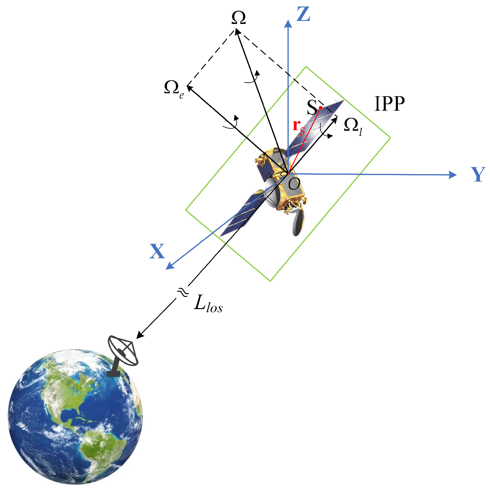
Figure 1. ISAR observation geometry.
Remotesensing 15 00033 g001
Figure 2. Various deformations of ISAR image for the same target. (a) Referenced ISAR image, (b) ISAR image azimuth scaling caused by accumulation angle, (c) ISAR image range scaling caused by radar bandwidth, (d) ISAR image rotation caused by target rotational motion, and (e) ISAR image deformation caused by the variation of main scattering centers.
Remotesensing 15 00033 g002
Figure 3. General flow chart of the training of CLISAR-Net.
Remotesensing 15 00033 g003
Figure 4. Structure of the encoder for obtaining deep representations of deformation ISAR images in CLISAR-Net.
Remotesensing 15 00033 g004
Figure 5. Illustration of 3 × 3 deformable convolution.
Remotesensing 15 00033 g005
Figure 6. The optimization flow of the encoder in CLISAR-Net. The update of base encoder is realized by backpropagation of the InfoNCE loss, and the momentum encoder is updated in a momentum way.
Remotesensing 15 00033 g006
Figure 7. Diagram of classifier fine-tuning in CLISAR-Net.
Remotesensing 15 00033 g007
Figure 8. The optical images, CAD models, and ISAR images of (a) CALIPSO, (b) Cloudsat, (c) Jason-3, and (d) OCO-2.
Remotesensing 15 00033 g008
Figure 9. Illustrations of the data augmentation operators. (a) Original, (b) rotated, (c) scaled down, (d) scaled up, (e) horizontal flip, (f) vertical flip, (g) center crop, resize, and horizontal flip, and (h) normalized ISAR image.
Remotesensing 15 00033 g009
Figure 10. Comparisons of involved methods on three datasets. (a) Classification results using 5% of labeled training samples and (b) classification results using 100% of labeled training samples.
Remotesensing 15 00033 g010
Figure 11. Comparison of the classification accuracy with different ratios of labeled training samples for different methods. (a) Results of scaled dataset, (b) results of rotated dataset, and (c) results of combined dataset.
Remotesensing 15 00033 g011
Figure 12. Classification accuracy of CLISAR-Net when different ranges of the azimuth angle are included in the training set of the combined deformation dataset.
Remotesensing 15 00033 g012
Figure 13. T-SNE visualization of the features for the combined deformation dataset from (a) input images, (b) pretraining of CLISAR-Net, (c) fine-tuning of CLISAR-Net, and (d) CNN-BiLSTM.
Remotesensing 15 00033 g013
Table 1. Detailed parameter settings of training and test sets for scaled deformation dataset.
ClassTraining SetTest Set
Δ θ = 5 , B = 1 GHz φ 1 , γ = 0 359 Δ θ = 6 , B = 2 GHz φ 1 , γ = 0 359 Δ θ = 6 , B = 1 . 5 GHz φ 1 , γ = 0 359 Δ θ = 4 , B = 2 GHz φ 1 , γ = 0 359
CALIPSO355354354356
Cloudsat355354354356
Jason-3355354354356
OCO-2355354354356
Total number28362840
Table 2. Detailed parameter settings of training and test sets for the rotated deformation dataset.
ClassTraining SetTest Set
Δ θ = 5 , B = 1 GHz φ 1 , γ = 90 359 Δ θ = 6 , B = 2 GHz φ 1 , γ = 90 359 Δ θ = 5 , B = 1 GHz φ 2 , γ = 0 359 Δ θ = 6 , B = 2 GHz φ 2 , γ = 0 359
CALIPSO265264355354
Cloudsat265264355354
Jason-3265264355354
OCO-2265264355354
Total number21162836
Table 3. Detailed parameter settings of training and test sets for the combined deformation dataset.
ClassTraining SetTest Set
Δ θ = 5 , B = 1 GHz φ 1 , γ = 90 359 Δ θ = 6 , B = 2 GHz φ 1 , γ = 90 359 Δ θ = 6 , B = 1 . 5 GHz φ 2 , γ = 0 359 Δ θ = 4 , B = 2 GHz φ 2 , γ = 0 359
CALIPSO265264354356
Cloudsat265264354356
Jason-3265264354356
OCO-2265264354356
Total number21162840
Table 4. Classification accuracy (%) of CLISAR-Net and other methods using 5% and 100% of labeled training samples on the three datasets.
MethodsTraining with 5% of Labeled SamplesTraining with 100% of Labeled Samples
Scaled Data.Rotated Data.Combined Data.Scaled Data.Rotated Data.Combined Data.
CNN77.5073.5971.8791.5887.9884.96
ST-CNN82.7178.7776.6293.6989.7786.65
Deform-CNN83.2178.2375.9693.7388.6886.58
CNN-BiLSTM86.3482.7880.8294.3392.5891.73
SVM87.5484.6982.6495.8193.7292.39
CLISAR-Net91.3486.6184.2398.1096.3795.85
Table 5. Comparisons of the number of trainable parameters and inference time between CLISAR-Net and existing methods.
MethodsNumber of Parameters (K)Inference Time (ms)
CNN124.380.0834
ST-CNN374.410.1862
Deform-CNN146.280.1031
CNN-BiLSTM326.780.0932
SVM/0.0196
CLISAR-Net267.730.1125
Disclaimer/Publisher’s Note: The statements, opinions and data contained in all publications are solely those of the individual author(s) and contributor(s) and not of MDPI and/or the editor(s). MDPI and/or the editor(s) disclaim responsibility for any injury to people or property resulting from any ideas, methods, instructions or products referred to in the content.