Stratospheric Aerosol Characteristics from the 2017–2019 Volcanic Eruptions Using the SAGE III/ISS Observations

Abstract

In recent years (2017–2019), several moderate volcanic eruptions and wildfires have perturbed the stratospheric composition and concentration with distinct implications on radiative forcing and climate. The Stratospheric Aerosol and Gas Experiment III instruments onboard the International Space Station (SAGE III/ISS) have been providing aerosol extinction coefficient (EC) profiles at multiple wavelengths since June 2017. In this study, a method to invert the spectral stratospheric aerosol optical depth (sAOD) or EC values from SAGE III/ISS (to retrieve the number/volume size distributions and other microphysical properties) is presented, and the sensitivity of these retrievals is evaluated. It was found that the retrievals are strongly dependent on the choices of wavelengths, which in turn determine the shapes of the calculated curves. Further, we examine the changes in stratospheric aerosol spectral behavior, size distribution properties, time evolution (growth/decay) characteristics associated with subsequent moderate volcanic eruptions, namely, Ambae (15${}^{\circ }$S, 167${}^{\circ }$E; April and July 2018), Raikoke (48${}^{\circ }$N, 153${}^{\circ }$E; June 2019), and Ulawun (5${}^{\circ }$S, 151${}^{\circ }$E; June and August 2019), in different spatial regions. The observational period was classified with reference to Ambae eruptions into four phases (pre-Ambae, Ambae1, Ambae2, and post-Ambae). The pre-Ambae and post-Ambe periods comprise the 2017 Canadian fires and 2019 Raikoke/Ulawun eruptions, respectively. The spectral dependence of sAOD was comparable and lowest during the pre-Ambae and Ambae1 periods in all regions. The number concentration at the principal mode radius (between 0.07 and 0.2 $\mathsf{\mu }$m) was observed to be higher during the Ambae2 period over the Northern Hemisphere (NH). The rate of change (growth/decay) in the sAOD on a global scale resembled the changes in the Southern Hemisphere (SH), unlike the time-lag-associated changes in the NH. These differences could be attributed to the prevailing horizontal and vertical dispersion mechanisms in the respective regions. Lastly, the radiative forcing estimates of Ambae and Raikoke/Ulawun eruptions, as reported in recent studies, was discussed by taking clues from other major and moderate eruptions to gain insight on their role in climate change.

1. Introduction

Volcanic eruptions are unpredictable episodic events that can have significant impacts on the global climate by altering the stratospheric composition, vertical temperature profiles, radiative processes, large-scale circulation, transport, and surface weather [1,2,3,4,5,6,7,8,9]. Although large magnitude eruptions with a volcanic explosivity index (VEI) equal to or greater than 5 (also known as Plinian eruptions), injecting around 10 Tg of sulfur dioxide (SO${}_2$), are rare on a decadal scale, they have a profound impact on the key modes of climate variability [10,11]. On the other hand, moderate magnitude volcanic eruptions (VEI ∼3–4, i.e., volume smaller than 1 km${}^3$ and total mass smaller than 1 Tg SO${}_2$) with a return frequency on the order of the year can still affect Earth’s temperature and radiation balance [12,13]. In both scenarios, the stratospheric aerosols originating from these volcanic events result in transitory perturbations. As a result, the net radiative energy balance [14] is sensitive to the aerosol composition [15,16,17] and microphysical characteristics (e.g., size distribution) [18,19], which are highly nonlinear. Furthermore, relatively small/medium events (VEI ≤ 4) during the past two decades have significantly contributed to the stratospheric aerosol loading, composition, stratospheric chemistry [20,21], and radiative forcing [22,23,24].

Despite the fact that long-term ground-based and balloon-borne instrumental observations are vital in understanding the microphysical evolution and optical properties of volcanic aerosols [25,26,27,28,29], they have limitations in terms of global coverage and other operational constraints. In this context, satellite observations have been providing reliable vertically resolved stratospheric aerosol spectral extinction data [18,24,30,31,32]. Among the various space-borne missions, the Stratospheric Aerosol and Gas Experiment on board the International Space Station (SAGE-III/ISS), the Ozone Mapping Profiler Suite Limb Profiler (OMPS-LP) onboard the Suomi National Polar-Orbiting Partnership satellite, and the Cloud-Aerosol LiDAR and Infrared Pathfinder Satellite Observations (CALIOP) are widely used to retrieve the stratospheric aerosol extinction. By comparing the retrieved extinction between OMPS-LP and SAGE-III/ISS, a systematically higher extinction from OMPS-LP (at altitudes above 28 km) and significant biases (up to ±13%) that were systematically lower than 19 km in the tropics were found [33]. In another study, CALIOP level 3 stratospheric aerosol retrievals were assessed with those from the SAGE III/ISS and it was found that the averaged differences between zonal mean extinction profiles were less than 25% between 20 and 30 km, exceeded 100% in the very low aerosol loading regimes above 25 km at higher latitudes, and ≥ 100% within 2 to 3 km above the tropopause altitude, possibly owing to cloud contamination [34]. Furthermore, Malinina et al. [18] emphasized that aerosol extinction retrievals were more accurate from occultation measurements (e.g., SAGE III/ISS) than those from limb instruments (e.g. OMPS-LP).

Several studies focusing on volcanic plumes in the upper troposphere and lower stratosphere (UTLS) regions provided information about the particle shape and size (useful for distinguishing volcanic ash, sulfate aerosol layers, and ice clouds) using the depolarization and color ratios (the ratio between 1064 and 532 nm backscatter signals) derived from the CALIOP and ground-based LiDAR, e.g., [28,32,35]. Renard et al. [36] proposed a color index based on in situ extinction measurements at 400 and 675 nm to obtain the vertical distributions of different stratospheric aerosol types, which can qualitatively indicate the changing nature of the aerosol population with altitude. All of these LiDAR and in situ techniques are limited by the number of wavelength channels at which extinction measurements are obtained. In this context, reliable retrievals of extinction spectra at multiple wavelengths from occultation measurements (e.g., SAGE III/ISS) provide a wider scope for the inversion of extinction spectra into size distributions (number/volume) and other integral properties (e.g. effective radius). Previously, different approaches for deducing stratospheric aerosol surface area density [37,38], size distributions, and integral properties [39,40], and the extinction ratio (between 525 nm and 1020 nm) existed to roughly infer the sizes of particles that dominate the extinction spectra from SAGE II. While the extinction ratio method [19] has been applied to SAGE III/ISS-based aerosol extinction spectra, there have been no attempts to infer the size distribution, which is one of the crucial parameters in modeling the radiative forcing of aerosols and in evaluating aerosol effects on ozone depletion caused by heterogeneous chemical reactions. So, the present study provides an inversion method to infer the size distributions and integrated properties using the extinction spectra from SAGE III/ISS by taking hints from previous methods, e.g., [39,40,41].

Among the recent volcanic events, the Ambae volcano (15${}^{\circ }$S, 167${}^{\circ }$E; VEI ∼3), which erupted twice on 5–6 April and 27 July 2018, injecting volcanic plumes into the UTLS region. While the April eruption had an impact on SH alone, the plume from the July eruption extended to both hemispheres through the lower branch of Brewer–Dobson circulation. In fact, the Ambae eruption was the onset of a series of even stronger and record-breaking moderate volcanic eruptions (for example, Raikoke/Ulawun in 2019 [24], and Hunga Tonga in 2022 [29,42]). Kloss et al. [30] discussed in detail the dispersion (horizontal, latitudinal, and vertical) of the Ambae aerosol plume in the UTLS region in addition to the optical properties and the global impact on the radiative balance. From the time of the Ambae eruption (April 2018) to the time of the Raikoke (48${}^{\circ }$N, 153${}^{\circ }$E; June 2019) and Ulawun (5${}^{\circ }$S, 151${}^{\circ }$E; June and August 2019) eruptions, no other significant stratospheric aerosol injections occurred, which could possibly interfere with the interpretation of results. The aerosol plumes originating from the Canadian wildfires (August 2017) were seen at higher latitudes (>40${}^{\circ }$N, ∼17 km) at the end of August 2017 confining above the Asian monsoon anticyclone (AMA) region until the end of June 2018 during which the plume was transported to the tropics via the eastern flank of AMA circulation [30,43]. Both the Ambae eruptions in 2018 were clearly distinguishable in SAGE III/ISS data, with the later eruption (July 2018) being much more intense than the earlier one (April 2018) [19]. Although the above studies dealt with some of the prominent aspects related to the Ambae (2018) and Raikoke/Ulawun (2019) eruptions, the present study is different in that it mainly introduces a method to invert the spectral values of the stratospheric aerosol optical depth(s) (sAOD) or extinction coefficients at particular altitudes into number/volume size distributions and other microphysical properties. We examined the changes in stratospheric aerosol spectral dependence, size-distribution properties, and time evolution characteristics (growth/decay) of Ambae eruptions. Lastly, the radiative forcing estimates of Ambae and Raikoke/Ulawun eruptions, as reported in recent studies, was discussed by taking clues from extensive studies carried out on El Chichón (1982), Nevado del Ruiz (1985), Pinatubo (1991), and other prominent eruptions to gain insight into their roles in climate change.

2. Data Set and Study Regions

2.1. SAGE III/ISS Data

The SAGE III/ISS conducts solar and lunar occultation measurements globally while orbiting the Earth. Vertical profiles of aerosol extinction were obtained using the rays passing through the atmosphere during sunrise/moonrise and sunset/moonset events. These aerosol extinction coefficient profiles (available since June 2017, Version 5.2; https://asdc.larc.nasa.gov/project/SAGE%20III-ISS, accessed on 28 June 2022) are retrieved at multiple wavelengths from ultraviolet to the near-infrared (384, 449, 521, 602, 676, 756, 869, 1021, and 1544 nm) from 0.5 km (or cloud top) to 40 km altitude with a vertical resolution of ∼1 km being reported in 0.5 km increments between 60${}^{\circ }$S and 60${}^{\circ }$N. Since the aerosol extinction information is unavailable in the lunar occultation product of SAGE III/ISS, only the solar occultation product (Level 2 Solar Event Species Profiles, V052, 0.5 km vertical interval) is used in this study. The volcanic plume was identified from the averaged SAGE III/ISS vertical profiles using a criterion based on the vertical variability of the computed Angstrom Exponent (AE) with the aerosol extinction measurements at 449 and 869 nm, while the cloud-contaminated extinction values were excluded when the ratio of extinction coefficients at 521 and 1021 nm was found to be less than 2 [30]. Apart from this, the tropopause altitude information from the MERRA-2 reanalysis (Modern-Era Retrospective analysis for Research and Applications, Version 2) included within the SAGE III/ISS data is used.

The sAOD is calculated by integrating the extinction coefficient profile from above the tropopause altitude to 30 km at the specified wavelength. Since the aerosol extinction at 521 nm is biased below 20 km due to an error in th O${}_4$ absorption cross-section [44] used in version 5.2 of SAGE III/ISS data, we replaced the sAOD values at 521 nm with interpolations of the corresponding sAOD values at 449 and 869 nm using a simple Angstrom coefficient scheme [19]. The extinction coefficient at 384 nm has a systematic bias in the UTLS region because of large molecular scattering contributions [40,45]. Therefore, the data at 384 nm were avoided in this study.

2.2. Study Regions

In this study, we categorized the SAGE III/ISS data into the following regions: Northern Hemisphere (NH; 0–60${}^{\circ }$N), Southern Hemisphere (SH; 0–60${}^{\circ }$S), and global (60${}^{\circ }$N to 60${}^{\circ }$S). Assuming that the variation with the longitudinal band is much smaller than the variation with the latitudinal band because of efficient mixing in the zonal direction and strong horizontal transport during the Ambae eruption periods, the daily average data for two latitude bins, namely, 10–20${}^{\circ }$S (covering the Ambae or Aoba volcanic island located in the central sector of the Vanuatu archipelago; 167${}^{\circ }$E, 15${}^{\circ }$S), and 10–20${}^{\circ }$N were taken into consideration for a better understanding of the background aerosol situations in different time periods. Note that SAGE III/ISS does not obtain measurements poleward of 60${}^{\circ }$.

3. Method

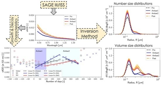
3.1. Inversion of Spectral sAOD Values into Aerosol Number/Volume Size Distributions

Stratospheric aerosols are most commonly represented by spherical droplets consisting of 25% H${}_2$O and 75% H${}_2$SO${}_4$ with log-normal particle size distributions [46]. There is still no evidence that any particular shape of the aerosol size distribution (including gamma distribution) provide better or worse physical descriptions of aerosol [33,47]. Historically, background stratospheric aerosols were represented by a monomodal log-normal size distribution while the post-volcanic aerosols (during the periods of high volcanism) were better represented with either bimodal [48] or even trimodal [49] log-normal size distributions. Several studies employing satellite-based measurements most commonly consider a monomodal log-normal distribution, e.g., [27,45,50]. In contrast, Yue [39,40] approximated the number-size distribution using a histogram and successfully retrieved the size distribution without assuming mono- or bi-modal distributions. In this study, we developed a flexible retrieval method without the assumption of mono- or bi-modal distributions. Our method is based on the retrieval technique of tropospheric aerosols from the measurements of AOD by a sun photometer, and the number-size distribution is assumed to be a combination of multiple log-normal distributions with fixed median radii and standard deviations, e.g., [41,51,52,53].

In order to retrieve the aerosol size distribution from the spectral values of stratospheric aerosol optical depth (sAOD) or extinction coefficient (EC) at a particular altitude level, the following assumptions are considered:

i.

The refractive index of stratospheric sulfate is assumed to be 1.45-i0 at all wavelengths [54].

ii.

The size distribution consisting of multiple log-normal distributions is considered as below:

$$\frac{dN\left(r\right)}{dlnr}=\sum _{i=1}^M{N}_{i}exp\left[-\frac{1}{2}{\left(\frac{lnr-ln{r}_{m,i}}{lns}\right)}^2\right]$$

(1)

where M is the number of log-normal distributions and is the same as the number of wavelengths at which sAOD values are considered, r is the particle radius ($\mathsf{\mu }$m), $r_{m,i}$ is the median (or mode) radius ($\mathsf{\mu }$m), s is the standard deviation of the $\frac{dN\left(r\right)}{dlnr}$ function, and $N_i$ is the parameter to be retrieved and is defined as the $\frac{N_0}{\sqrt{2\pi }lns}$. Here, N${}_0$ is an integrated value of the i^th log-normal function. The median radius ($r_{m,i}$) and standard deviation (s) are given from $r_{min}$ (= 0.1 $\mathsf{\mu }$m) to $r_{max}$ (= 1.0 $\mathsf{\mu }$m) as below:

$$r_{m,i}=exp\left[ln{r}_{min}+(i-0.5)\Delta lnr\right],i=1,....,M$$

(2)

$$s=exp\left(\Delta lnr/1.65\right)$$

(3)

$$\Delta lnr=ln\left(r_{max}/r_{min}\right)/M$$

(4)

In this study, the wavelengths used in the retrieval are 449, 521, 602, 676, 756, 869, 1021, and 1544 nm, and M is fixed as 8 (i.e., equal to the number of wavelengths). The logarithm of $r_{m,i}$ is equally spaced with $\Delta lnr$. The value of s depends on M, and is fixed at 1.221 for each log-normal distribution. The choice of $r_{min}$ or $r_{max}$ constrains the retrieval values of s and $r_{m,i}$. The factor of 1.65 is empirically determined [41,55]. All of the log-normal distributions are assumed to have the same standard deviation s. The log value of this constant standard deviation is assumed to be proportional to 1/M. Thus, more distribution means a smaller s. The retrieval range of the particle radius is kept fixed from 0.1 $\mathsf{\mu }$m ($r_{min}$) to 1.0 $\mathsf{\mu }$m ($r_{max}$) [39,40]. In earlier studies, for example, by King et al. [52] and Kudo et al. [41], it was found that a satisfactory size distribution can be derived for the radius range between 0.1 and 1.0 $\mathsf{\mu }$m if the sAOD or EC values are available throughout the visible and near-infrared wavelength regions. Therefore, $r_{m,i}$ is fixed at 0.118, 0.164, 0.228, 0.316, 0.439, 0.611, and 0.848 $\mathsf{\mu }$m for each log-normal distribution. Now, the only free parameters in the inversion procedure are the $N_i$.

iii.

Optical properties of spherical particles are calculated using the Mie theory.

The parameter $N_i$ (where $i=1,...M$) is optimized to the measured sAOD or EC (at each wavelength) by the maximum likelihood method. The best estimate was obtained by minimizing the cost function given below:

$$f\left(x\right)={(ln\left({\mathbf{y}}^{obs}\right)-ln\left(\mathbf{y}\left(\mathbf{x}\right)\right))}^T{\left({\mathbf{W}}^2\right)}^{-1}(ln\left({\mathbf{y}}^{obs}\right)-ln\left(\mathbf{y}\left(\mathbf{x}\right)\right))+{\mathbf{y}}_a{\left(\mathbf{x}\right)}^T{\left({\mathbf{W}}_a^2\right)}^{-1}{\mathbf{y}}_a\left(\mathbf{x}\right)$$

(5)

where $\mathbf{x}$ is ${\mathbf{N}}_i$ of Equation (1), ${\mathbf{y}}^{obs}$ is the measurement of sAOD or EC, $\mathbf{y}\left(\mathbf{x}\right)$ is the forward model for calculating sAOD or EC from $\mathbf{x}$, ${\mathbf{W}}^2$ is the covariance matrix (assumed to be diagonal), and the measurement accuracy of sAOD or EC is assumed to be 5% (refer to Table 4 at https://www.eoportal.org/satellite-missions/iss-sage-3#ground-system; accessed on 28 June 2022). The vector ${\mathbf{y}}_a$ is the smoothness constraint for the size distribution and is given below:

$${\mathbf{y}}_a\left(\mathbf{x}\right)=ln\left(N_{i-1}\right)-2ln\left(N_i\right)+ln\left(N_{i+1}\right)$$

(6)

where $i=2,...,M-1$. The covariance matrix ${\mathbf{W}}_a^2$ is assumed to be diagonal and is the weight to determine the strength of the smoothness constraint. The best estimate of $\mathbf{x}$, which minimizes f($\mathbf{x}$), was obtained by iterations using the Gauss-Newton and line search methods [56]. The retrieval errors of the optimized $\mathbf{x}$ due to the random errors of ${\mathbf{y}}^{obs}$ were estimated using the method described by Dubovik et al. [53]. Assuming the linear dependencies of the retrieval errors on the measurement errors, the covariance matrix of the retrieval errors is expressed as below:

$${\mathbf{C}}_x={({\mathbf{U}}_x^T{\left({\mathbf{W}}^2\right)}^{-1}{\mathbf{U}}_x+{\mathbf{U}}_{a,x}^T{\left({\mathbf{W}}_a^2\right)}^{-1}{\mathbf{U}}_{a,x})}^{-1}{ϵ}^2$$

(7)

where ${\mathbf{U}}_x$ and ${\mathbf{U}}_{a,x}$ are the Jacobi matrices of the first derivatives for $ln\left(\mathbf{y}\left(\mathbf{x}\right)\right)$ and $y_a\left(\mathbf{x}\right)$, respectively, in the vicinity of the optimized $\mathbf{x}$. The variance of measurement errors, ${ϵ}^2$, is estimated from the residual value, which is the obtained minimum of the quadratic form $f\left(\mathbf{x}\right)$ (Equation (5)), and is estimated as below:

$${ϵ}^2\approx \frac{f\left(\mathbf{x}\right)}{(M_y-M_x)}$$

(8)

where $M_y$ is the number of sAOD measurements and the a priori smoothness constraint, and $M_x$ is the number of retrieved parameters. Finally, the retrieval errors of $\mathbf{x}$ are estimated by taking the diagonal elements of ${\mathbf{C}}_x$.

Using the method outlined above, the aerosol microphysical parameters to be estimated include the effective radius (R${}_{eff}$, in $\mathsf{\mu }$m), volume ($dV\left(r\right)/dlnr$ in $\mathsf{\mu }$m${}^3$/$\mathsf{\mu }$m${}^2$) and number-size distributions ($dN\left(r\right)/dlnr$ in 1/$\mathsf{\mu }$m${}^2$). Both the volume and number-size distributions are related as following:

$$\frac{dV\left(r\right)}{dlnr}=V\left(r\right)\frac{dN\left(r\right)}{dlnr}=\frac{4}{3}\pi r^3\frac{dN\left(r\right)}{dlnr}$$

(9)

To better quantify the differences in the entire size distribution, a parameter that is often used to denote the particle size is the effective (or area-weighted) radius (R${}_{eff}$), defined as the third moment of the aerosol size distribution over the second moment. This is represented as below:

$$R_{eff}=\frac{M_3}{M_2}=3\left(\frac{V}{S}\right)$$

(10)

where the n^th size distribution moment, $M_n$, is defined as below:

$$M_n={\int }_0^{\infty }\frac{dN\left(r\right)}{dlnr}{r}^{n}dlnr$$

(11)

with the second and third moments corresponding to the aerosol surface area (S) and volume (V) densities, respectively, defined as below:

$$S={\int }_0^{\infty }4\pi r^2\frac{dN\left(r\right)}{dlnr}dlnr$$

(12)

$$V={\int }_0^{\infty }\frac{4}{3}\pi r^3\frac{dN\left(r\right)}{dlnr}dlnr$$

(13)

Discrepancies in the retrieved effective radius (R${}_{eff}$) can arise because of the assumption of the refractive index, although this will not have any significant effect on the shape of the retrieved size distribution. The refractive index mainly affects the integrated properties, such as the R${}_{eff}$. An average error of 2–9% in the R${}_{eff}$ was reported by assuming the true particle refractive index to be constant [57]. The errors in the volume and number-size distributions, as well as R${}_{eff}$, were estimated from the retrieval errors of $\mathbf{x}$.

3.2. Retrieval Assessment

In order to ascertain the performance of our inversion method, the simulated sAOD from the six size distributions of Yue [39,40] were considered (listed in

Table 1. Parameters of the six log-normal size distributions of Yue [39,40] used in this study. The first and second columns below the retrieved R${}_{eff}$ correspond to sAOD (at 521 nm) = 0.005 and 0.001, respectively. The number of N${}_i$ is fixed by 8 in all of the retrieval results because the number of wavelengths is 8.

Model	Type	N${}_1$/N${}_2$	r${}_{\mathit{m},1}$	r${}_{\mathit{m},2}$	${\mathit{s}}_1$	${\mathit{s}}_2$	Simulated	Retrieved
			($\mathsf{\mu }$m)	($\mathsf{\mu }$m)			R${}_{\mathit{eff}}$	R${}_{\mathit{eff}}$	R${}_{\mathit{eff}}$
							($\mathsf{\mu }$m)	($\mathsf{\mu }$m)	($\mathsf{\mu }$m)
A	Monomodal	1.00	0.07	–	1.86	–	0.19	0.22	0.21
	(N${}_1$ = N${}_2$)
B	Monomodal	1.00	0.09	–	1.80	–	0.21	0.23	0.21
	(N${}_1$ = N${}_2$)
C	Bimodal	1.76	0.11	0.43	1.67	1.36	0.50	0.49	0.53
D	Bimodal	1.41	0.11	0.30	1.43	1.48	0.40	0.39	0.38
E	Bimodal	0.98	0.13	0.56	1.58	1.26	0.61	0.62	0.64
F	Bimodal	0.76	0.09	0.39	1.41	1.30	0.45	0.44	0.42

). The log-normal size distributions of monomodal/bimodal shapes were obtained using the parameters in Table 1. Assuming that the refractive index is 1.45-i0 at all of the wavelengths, sAOD values at 449, 521, 602, 676, 756, 869, 1021, and 1544 nm are computed with Mie calculations. The absolute values of $N_1$ and $N_2$ are adjusted to the simulated sAOD (at 521 nm) taken as 0.005 and 0.001, respectively.

Yue [40] showed that their method can be applied to various shapes of the size distributions and provided the sensitivity of different wavelength combinations of SAGE III/ISS measurements of retrieved size distributions at different altitude ranges. It was found that the EC values at eight wavelengths (384 to 1544 nm) for 15–40 km, and seven wavelengths (449 to 1544 nm) for 10–15 km are necessary for retrieving the size distributions with minimal uncertainties. Recently, Wrana et al. [45] emphasized the strong dependence of the extinction ratio on the particle size and choice of wavelength combinations. They found that the EC at 384 nm channel causes systematic bias in the UTLS region because of the large molecular scattering contributions. Further, they suggest the usage of 1544 nm channel for broad wavelength interval and for better accuracy in order to compensate the higher extinction ratio uncertainties. So, the measurements corresponding to the wavelength intervals from 449 to 1544 nm are taken into account while those in the 384 nm channel are avoided. In this study, we performed the sensitivity of sAOD or EC values corresponding to both wavelength ranges, and found that the measurements of 448 to 1544 nm exhibited the lowest root mean square error (RMSE) between the retrieved and simulated (Table 1) size distributions. Figure 1 shows the retrieval results of the number and volume size distributions for models A–F with the simulated sAOD (at 521 nm) of 0.005. We find that our method is able to retrieve both monomodal and bimodal size distributions. However, the retrieved number-size distributions at the radii from 0.1 to 0.2 $\mathsf{\mu }$m (Figure 1 b,e,h,k,n,q) were overestimated, and the errors were greater than the expected retrieval uncertainties. According to the Mie theory, the size parameters for the wavelengths from 449 to 1544 nm and the particle radii from 0.1 to 0.2 $\mathsf{\mu }$m were from 0.4 to 2.5, and the extinction efficiencies were smaller than those of the particles with radii greater than 0.2 $\mathsf{\mu }$m. Therefore, the contributions of the particles at radii less than 0.2 $\mathsf{\mu }$m to the sAOD at the wavelengths from 449 to 1544 nm were small, and the size distributions at radii less than 0.2 $\mathsf{\mu }$m were not retrieved accurately. As a result, the retrievals tended to overestimate the fine mode. Earlier, Deshler et al. [58] reported that the measurement uncertainties can lead to an error of the fits by ±20%, ±30%, and ±40%, respectively, for the geometric width (s), median radius (r${}_m$), surface area (S), and volume (V) densities. We found that the measurement accuracy of sAOD is always less than 5%.

The retrieved volume size distributions (Figure 1c,f,i,l,o,r) exhibited monomodal shapes that are concurrent with those from models A–F. The retrieved R${}_{eff}$ values obtained with sAOD (at 521 nm) fixed at 0.005 and 0.001 for models A–F are given in Table 1. The simulated R${}_{eff}$ values in both cases of fixed sAOD (at 521 nm) remained similar for each model (A–F). The differences in R${}_{eff}$ corresponding to models A–F (simulated) and those retrieved were less than equal to 0.03 $\mathsf{\mu }$m, with a maximum deviation of ±15%. Although our method exhibited consistency with both monomodal and bimodal number/volume size distribution shapes, the fine mode was overestimated. This might affect the results of the total number concentrations. However, the overestimated fine mode has a little influence on the retrieved R${}_{eff}$.

4. Results and Discussion

Based on the aerosol extinction coefficient profile data from SAGE III/ISS, sAOD was derived at different wavelengths (Section 2.1). These spectral sAOD values at 449, 521, 602, 676, 756, 869, 1021, and 1544 nm are used to invert the microphysical parameters of stratospheric aerosols (Section 3.1) in different regions (Section 2.2). In this study, we classified the entire time period of observational data set into four different phases, namely, (i) pre-Ambae (before Ambae eruption; July 2017–March 2018; major influence of the Canadian wildfire event in August 2017 at high northern latitudes >40${}^{\circ }$N, while a minor impact was perceived in the Asian monsoon anticyclone (AMA) region consisting of the southern part (5–38${}^{\circ }$N and 40–95${}^{\circ }$E)), (ii) Ambae1 (first Ambae eruption; 5 April–26 July 2018), (iii) Ambae2 (second Ambae eruption; 27 July 2018–21 June 2019), and (iv) post-Ambae (starting with the Raikoke eruption on 22 June 2019 and including the Ulawun eruption from 26 June/3 August 2019 to the end of January 2020). Here, it should be noted that the pre-Ambae period does not necessarily represent the non-volcanic (or background) conditions, and might variably influence the spectral and microphysical properties of stratospheric aerosols due to the 2017 Canadian wildfire plume in different regions.

4.1. Spatiotemporal Variability of Spectral Dependence and Size Distribution of Stratospheric Aerosols

Stratospheric aerosol levels, primarily influenced by volcanic eruptions, are mostly dominated with sulfuric acid droplets or with a mix of ash particles and sulfuric acid droplets or distinct layers [19,28]. The dynamical and microphysical processes together with varying composition in time lead to changes in the size distribution, which strongly influence the wavelength dependence of sAOD with further implications on the radiative properties.

Although the usual decreasing behavior of sAOD with increasing wavelengths is seen (Figure 2a,d,g,j,m), distinct magnitudes were noticed in different time periods over each of the selected regions and both the latitudinal bands. The spectral dependency of sAOD during the pre-Ambae and Ambae1 periods was found to be lower and comparable in respective regions. Surprisingly, the sAOD values at all wavelengths during the Ambae2 period in the NH region and 10–20${}^{\circ }$N latitude band remained similar and close to the values observed during the pre-Ambae and Ambae1 periods, respectively. High pre-Ambae values in the NH were certainly due to the impact of the 2017 Canadian fire plume. In contrast, the sAOD values at shorter wavelength regime increased in magnitude over SH and 10–20${}^{\circ }$S latitude band during the Ambae2 period compared to the pre-Ambae and Ambae1 periods. Subsequently, this increasing feature in shorter wavelength regime was also observed globally. During the post-Ambae period, distinct magnitudes of sAOD enhanced by 2–3 times at all wavelengths was seen in NH and global regions along with 10–20${}^{\circ }$N latitude band due to the perturbation of the stratospheric aerosol layer caused by the Raikoke eruption (June 2019). Slight enhancements of sAOD values at shorter wavelengths were found in the SH region and 10–20${}^{\circ }$S latitude band, possibly because of the Ulawun eruption (June and August 2019) and the transport of some parts of the Raikoke plume. Interestingly, large variability around the mean sAOD values can be seen over both the latitude bands during the post-Ambae period indicating the likely influence of large stratospheric perturbation associated with two distant volcanic eruptions at nearly the same time.

The log-normal number-size distributions of stratospheric aerosols inverted from the spectral sAOD values were found to be mostly dominated by the monomodal distributions between 0.07 and 0.2 $\mathsf{\mu }$m with the peak at around 0.12 $\mathsf{\mu }$m (Figure 2b,e,h,k,n). Similar shapes (first and principal mode) were noticed over all regions for pre-Ambae, Ambae1, Ambae2, and post-Ambae periods. We found that the total number concentration varied distinctly in different time periods (indicating the changing concentration levels) at each region although the geometric width and median radii did not differ significantly. The number concentration at the principal mode radius was found to be distinct and higher during the Ambae2 period followed by Ambae1, pre-Ambae and post-Ambae periods over the NH region clearly indicates the influence of the second Ambae eruption on stratospheric aerosol concentrations. Furthermore, the number concentrations at the principal mode radius during the pre-Ambae and Ambae1 periods were almost similar, indicating that the first Ambae eruption did not influence the NH region during the Ambae1 period. Although the magnitudes of the spectral sAOD values in the post-Ambae period were much higher than those observed during other time periods, the number concentration at the first principal mode remained lower because of the presence of a second mode centered around 0.3 $\mathsf{\mu }$m. In the other regions (SH, global, and two latitude bands), the number concentration at the principal mode radius was found to be the lowest during the pre-Ambae period followed by increases in the Ambae1, Ambae2, and post-Ambae periods.

The log-normal volume size distributions exhibited mostly bi-modal and tri-modal shapes, with distinct differences in each region during different time periods (Figure 2 c,f,i,l,o). We found that including higher (1544 nm) and excluding smaller (384 nm) wavelengths tended to strongly modify the amplitude of the first mode and the shapes of the second and third modes (figure not shown). This was also emphasized by Wrana et al. [45] that the retrievals are strongly dependent on the choice of wavelengths, which in turn determines the shapes of the calculated curves. The first modes of both the number and volume size distributions followed similar patterns of the peak magnitudes during different time periods over each region. In contrast, distinct peak magnitudes at median radii and geometric widths were observed for the higher modes in all regions at different time periods. While the second mode was found to peak between 0.2 and 0.3 $\mathsf{\mu }$m, the third mode occurred between 0.5 and 0.7 $\mathsf{\mu }$m during the Ambae1 and Ambae2 periods, respectively. Large differences in the magnitude of the second mode between the Ambae2 and Ambae1 periods over SH and global regions (including the two latitude bands) indicating that particles in the size range of 0.2 to 0.4 $\mathsf{\mu }$m contributed significantly to the spectral sAOD values in those respective regions during the Ambae2 period. In case of NH, the peak volume of the first mode was observed to be higher while the second mode was similar during the Ambae2 period than that in the Ambae1 period, indicating the enhanced fine particle concentrations in the range of 0.1 to 0.16 $\mathsf{\mu }$m influencing the spectral pattern of the sAOD. For other regions, an almost comparable peak volume concentration was observed for the first modes during the Ambae1 and Ambae2 periods. Interestingly, the second mode was highly dominant with wider geometric width (compared to the first mode) during the post-Ambae period over NH and global regions while similar magnitudes of the first and second modes were perceived in the 10–20${}^{\circ }$N latitude band. This enhanced concentrations in a broader size range can be attributable to the perturbation in stratospheric aerosols due to the Raikoke eruption. In contrast, slight differences existed in the peak volume concentrations of the second modes between post-Ambae and Ambae2 periods in the SH although a higher magnitude was found during the post-Ambae period. This indicates the contribution of the Ulawun plume. Kloss et al. [24] suggested a more homogeneous small-sized sulfate aerosol composition of the Ulawun plume while the presence of either ash, carbonaceous, larger sulfate-coated ash, or carbonaceous particles were in the Raikoke plume. So, the presence of ash and carbonaceous particles would likely bias the size distribution retrieval, which is based on the refractive index of sulfate.

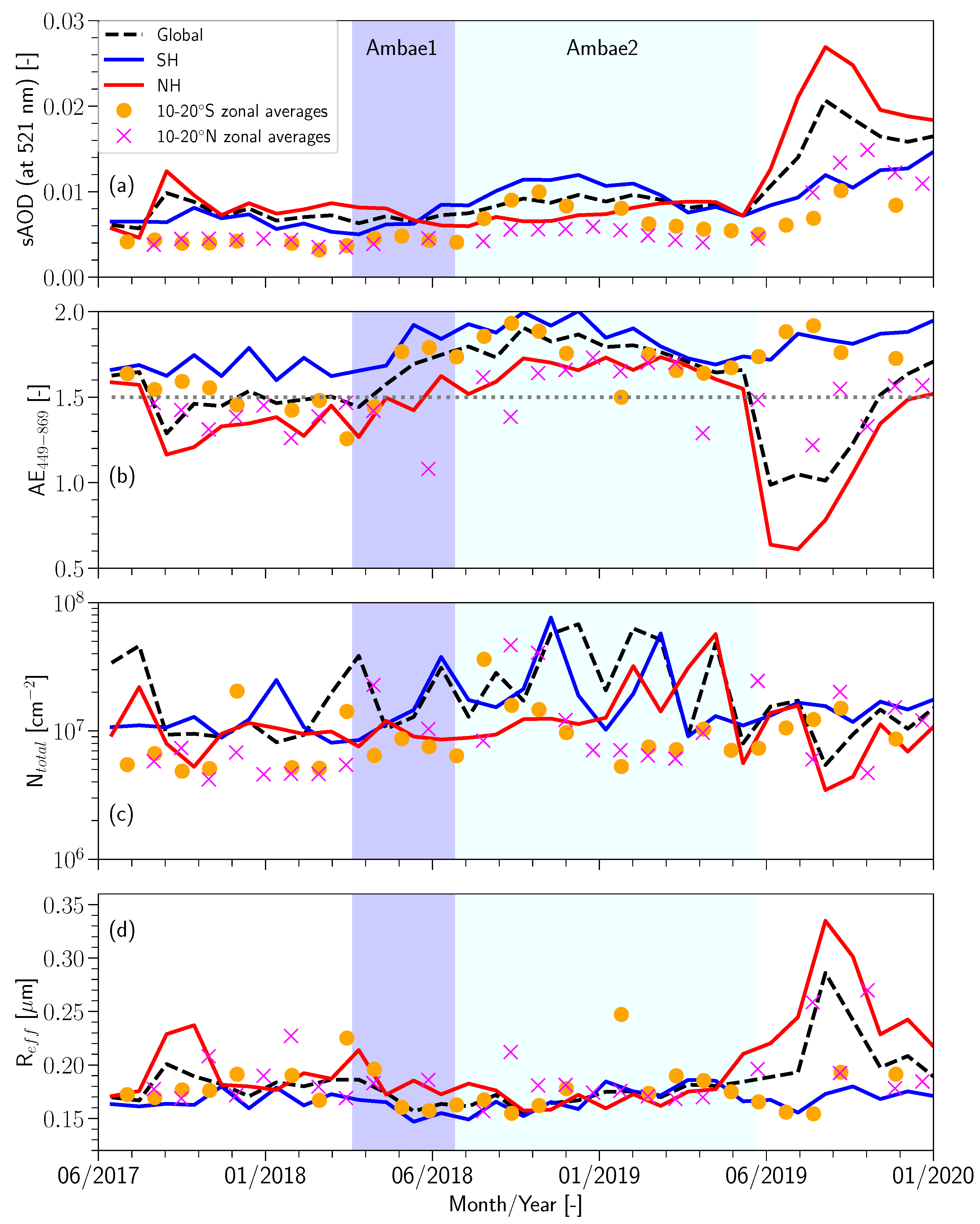
4.2. Temporal Changes in the sAOD, Angstrom Exponent, Total Number Concentration, and R${}_{eff}$

By comparing the time evolution of sAOD (at 521 nm) among the different regions (global, SH, and NH; Figure 3a), it was observed that the sAOD remained slightly higher in the NH followed by the values corresponding to the global and SH regions until mid-May 2018. The Canadian fire plume was seen in higher latitudes (>40${}^{\circ }$N) at the end of August 2017 in the lower stratosphere (∼17 km) above the AMA region (or Asian area), confined until the end of June 2018 (at ∼19 km) [30,43]. An enhancement in the sAOD was noticed over the SH with magnitudes remaining higher than those over the global and NH regions until March 2019 due to the Ambae eruptions. Thereafter, comparable magnitudes of sAOD was noticed among NH, SH, and global regions until the mid of May 2019 after which an abrupt increase in the sAOD was seen over NH (∼3.5 times) followed by global (∼2.75 times) and SH (∼1.75 times) regions in the post-Ambae period. Earlier, Kloss et al. [24] found that perturbation of the stratospheric aerosol layer (by producing larger particles than the background) due to the Raikoke eruption was significantly higher due to the Ulawun eruption. Interestingly, the temporal variation of sAOD corresponding to the latitude bands depicted similar patterns of behavior (with lower magnitudes) represented by their respective extended regions, namely NH and SH.

The AE${}_{449-869}$ values were observed to be >1.5 on a global scale during the first and second phases of Ambae eruptions while they were either lower than or close to 1.5 during the remaining periods (Figure 3b). An increase in the AE${}_{449-869}$ (approaching 2.0) indicates the dominance of a small sulfate aerosol composition in the stratosphere. However, the global mean values of AE${}_{449-869}$ remained lower (between 1.0 and 1.5) when the Raikoke and Ulawun eruptions occurred in June/August 2019 despite an abrupt increase in the sAOD values (at 521 nm) that are much higher (>1.5) than those prevalent during the Ambae1 and Ambae2 periods. In the NH, AE${}_{449-869}$ values were seen to be lowest (∼0.6 and above) during the post-Ambae period, possibly due to the influence of the Raikoke eruption, which was associated with comparatively larger particles, including ash [24].

Although the geometric width and median radius from the inverted log-normal number-size distributions did not differ much, the total number concentration (N${}_{total}$; Figure 3c) was fluctuating in different time periods. During the Ambae period (May 2018 to January 2019), strong fluctuations in N${}_{total}$ with almost concurrent patterns were noticed in the SH and global regions. For the post-Ambae period, the fluctuations in N${}_{total}$ have abruptly reduced in SH, while the concurrent patterns were noticed between NH and global regions. The strong fluctuations in N${}_{total}$ can be resulting because of the temporal variation in the spectral dependence of sAOD values. The retrieval algorithm does not have any constraints for the temporal variations. However, the overestimation of the fine mode can affect N${}_{total}$. It is physically possible that the Raikoke plume was characterized by a smaller second mode during the post-Ambae period over NH (there is some indication of that with in situ measurements at 17.5${}^{\circ }$N and 78.2${}^{\circ }$E on 18 July 2019 [30]) but this would differ from other reported plumes (Sarychev, Calbuco, and Hunga Tonga).

The stratospheric aerosol effective radius (R${}_{eff}$; Figure 3d) remains to be stable with no significant changes lying between 0.15 and 0.24 $\mathsf{\mu }$m during the pre-Ambae and Ambae periods in all regions. It is possible that the microphysical changes associated with Ambae plume were not evidently visible because the derived R${}_{eff}$ was obtained from the number-size distributions of spectral sAOD values corresponding to an altitude range. However, a drastic increase in R${}_{eff}$ reaching a peak value between 0.28 and 0.34 $\mathsf{\mu }$m (till the end of August 2019) was observed during the post-Ambae period in the NH, global, and 10–20${}^{\circ }$N latitude band. Interestingly, the increasing peak in R${}_{eff}$ and sAOD seems to be associated with the decreasing pattern exhibited by AE${}_{449-869}$ and N${}_{total}$ over the NH and global regions during the post-Ambae period. It is possible that the presence of ash, carbonaceous, larger sulfate-coated ash, or carbonaceous particles in the Raikoke plume [24] might have significant impacts during the post-Ambae periods over the NH and global regions.

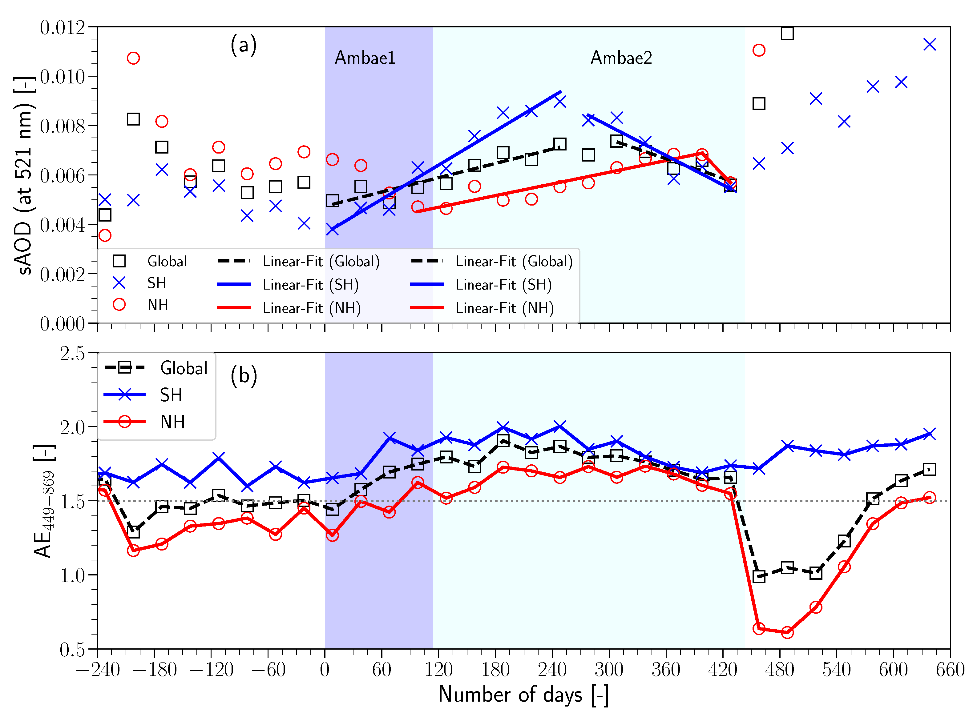
4.3. Growth and Decay Characteristics of sAOD and AE${}_{449-869}$

A steep increasing slope in the sAOD was observed (∼3.10 × 10${}^{-5}$ per day; Figure 4a) in the SH throughout the whole Ambe1 and Ambae2 periods (∼249 days). Thereafter, the decay phase started with a decrement in the sAOD at the rate of −2.60 × 10${}^{-5}$ per day until the previous day of the Raikoke eruption (i.e., 21 June 2019). Although a similar increasing slope in the sAOD was observed for global (∼1.40 × 10${}^{-5}$ per day) and NH (∼1.03 × 10${}^{-5}$ per day), they have different starting and ending days in both regions, indicating a time lag existed with respect to the dispersion from SH to NH. The rate of decrease in the sAOD was found to be more drastic in NH (−4.80 × 10${}^{-5}$ per day) than that in global (−1.80 × 10${}^{-5}$ per day) with different starting days (i.e., 8 May 2019 for NH, and 7 February 2019 for global) and the same ending day. Overall, the rate of change (growth/decay) in the sAOD over the SH seems to be clearly depicted in the changes associated with global consideration while there is a distinct time lag in the corresponding changes in the NH. From this, it is clearly evident that differences in the growth and decay periods of sAOD are a characteristic of prevailing horizontal and vertical dispersion mechanisms in different regions.

The AE${}_{449-869}$ (Figure 4b) was always higher than 1.6 in the SH. It was observed that AE${}_{449-869}$ approached close to 2.0 after 60 days from the date of the first Ambae volcanic eruptions, and remained at comparable values for almost 10 months. Afterward, these AE${}_{449-869}$ values were reduced to 1.7 and remained constant for the next 6 months. In the NH, AE${}_{449-869}$ values were observed between 1.2 and 1.5 in the first two months (∼60 days) after the first eruption. These AE${}_{449-869}$ values have increased above 1.5 and remained close to 1.8 for the next 300 days (∼10 months) to subsequently remain at 1.5 (by 21 June 2019) and further lower. Before the eruption of the Ambae volcano, the global AE${}_{449-869}$ values remained at 1.5. After the first eruption, the AE${}_{440-869}$ values increased steadily until the value was 1.9 and remained above 1.6 until 21 June 2019. These values are consistent with the reported average AE (calculated from the AOD values at 869 and 521 nm) between 0.9 (for the Canadian wildfire plume) and ∼1.9 (for the Asian tropopause aerosol layer, ATAL) in a study to trace the Canadian wildfire plume in the AMA region [43].

5. Radiative Impact of Ambae and Raikoke/Ulawun Eruptions with Other Well-Known Eruptions

To assess the radiative impacts caused by the Ambae (2018) and Raikoke/Ulawun (2019) eruptions with other well-known eruptions, we summarized the reported values (from the existing literature) of aerosol loading and radiative forcing (RF) in Table 2.

The Ambae eruption in July 2018 has resulted in the perturbation of sAOD values from 0.012 (at 449 nm) to 0.002 (at 1544 nm) on a global scale indicating a sensible perturbation of lower stratospheric aerosol extinction. These are consistent with the total sAOD (0.009 at 869 nm to 0.014 at 384 nm) reported by Kloss et al. [30]. Consequently, this perturbation was found to be comparable with the recent stratospheric eruptions (VEI ∼4 or 5; and with an SO${}_2$ total mass loading > 0.05 Tg), namely, Kasatochi (2008), Sarychev (2009), Nabro (2011) e.g., [1,54]. In the context that no eruption after 2016 has been classified as VEI > 4 until the most recent Hunga Tonga Ha’apai eruption (VEI 5–6) [59,60], the Ambae eruption (VEI ∼3) assumes significance due to the fact that it was found to exhibit comparable perturbations with other moderate eruptions (Kasatochi, Sarychev, and Nabro) [1]. Top of the Atmosphere (TOA) radiative forcing (RF) values estimated for Ambae eruptions (−0.45 to −0.60 W m${}^{-2}$) indicated the strongest climate impact for the year 2018 [30]. This RF is comparable with Kasatochi, Sarychev, and Nabro (−0.40 to −0.50 W m${}^{-2}$) [1,54]. In another study by Malinina et al. [31], it was found that, using ECHAM5 model simulations, an instantaneous RF (for tropical regions covering 20${}^{\circ }$N to 20${}^{\circ }$S) reached the maximum in the first week of September (−0.11 W m${}^{-2}$), and afterward declined slowly until December 2018 (up to −0.08 W m${}^{-2}$). They found the maximum RF in November 2018 (−0.22 W m${}^{-2}$) to further decrease by the end of the year (−0.19 W m${}^{-2}$). Lastly, they report that the instantaneous RF (tropical) caused by an increase in stratospheric aerosols to be around −0.13 W m${}^{-2}$, which was significantly lower than the TOA RF values reported by Kloss et al. [30]. The instantaneous RF provides a good approximation to the flux change at the TOA (and throughout the stratosphere) after the stratosphere is allowed to adjust radiatively owing to the presence of a forcing agent [61]. Even though they attribute the main reason for this disagreement can be from the differences in the approaches followed to subtract the non-Ambae signal in either of the methods and data sets used for estimating the RF, further differences might be possible from the comparison of RF estimates from empirical approximation [61] with those resulting from the type (i.e., online or offline) of radiative transfer calculations performed.

The Pinatubo eruption (1991) is significant for its climate impact in the twentieth century and was observed better than previous eruptions (e.g., 1982 El Chichon and 1985 Nevado del Ruiz). The forcing from Pinatubo is nearly symmetric between the two hemispheres, with a peak value of about −3 W m${}^{-2}$ near the equator. Moreover, the perturbation in visible flux was strongest (−4 to −5 W m${}^{-2}$) at the TOA and weaker (−3 to −4 W m${}^{-2}$) at the surface, while the infrared flux perturbation is stronger (−6 to −7 W m${}^{-2}$) at the tropopause [62]. Model simulation results of the Pinatubo eruption showed a global peak in the visible optical depth (∼0.15), yielding a negative perturbation of about −3 W m${}^{-2}$ [63]. The El Chichon eruption (April 1982) produced a negative RF of −2 to −4 W m${}^{-2}$ in the troposphere in just over a year [64] and the Pinatubo eruption resulted in a RF of $\sim -$4.5 W m${}^{-2}$ at the TOA over the 40${}^{\circ }$S to 40${}^{\circ }$N region [65]. From 2008 to 2011, the stratospheric volcanic aerosols imposed an aerosol RF of −0.11 (−0.15 to −0.08) W m${}^{-2}$ [66]. Moreover, Thomason et al. [19] found that the microphysical properties of the Ambae eruption are similar to those of the Nevado del Ruiz eruption (November 1985), corresponding to possible characteristics of small-to-moderate eruptions. Wang et al. [67] estimated the global forcing for Kasatochi eruption to obtain similar values at the surface and TOA. They have reported that the Kasatochi eruption has much less climate impact in spite of affecting the global radiative energy budget for approximately 100 days after the eruption. The RF estimates for Ambae eruption were relatively large, and negative TOA RF values were found to be comparable with those estimated for the Kasatochi, Sarychev, and Nabro eruptions. After the Ambae eruption, the Raikoke eruption was mostly confined to NH with the possible influence of ash in the evolution of sAOD whereas the Ulawun eruption had an impact on aerosol enhancements in both the tropics and SH. In comparison with Ambae (2018) and Ulawun (2019) eruptions, larger sAOD (∼0.04) and RF values at the TOA (−0.11 to −0.16 W m${}^{-2}$ and shortwave all-sky) were found for the Raikoke (2019) eruption [24]. Of late, the Hunga Tonga-Hunga Ha-apai (HT; 20.57${}^{\circ }$S, 175.38${}^{\circ }$W; 15 January 2022; VEI 5–6) [59,60] has displayed unexpected radiative impacts with the surface RF mainly contributed ti by the aerosol effect (close to −2 W m${}^{-2}$ [42]), which, in the last 30 years, can be considered a much higher hemispheric averaged surface impact for any stratospheric event. Nevertheless, the HT volcano also injected an unprecedented amount of water vapor into the deep stratosphere. The overall effect of stratospheric aerosol and water vapor perturbations by HT have been proposed to produce uncommon heating effects on the climate system [42]. Apart from these, extreme fire events like the Canadian wildfires of 2017 [43] and Australian Bushfires in 2019–2020 [68] are expected to occur more frequently elsewhere, leading to additional local heating in the layer along with a significant cooling effect on the climate system.

Table 2. List of significant volcanic eruptions with estimated aerosol loading and radiative forcing (RF), as reported in various published studies. The VEI values were obtained from https://www.usgs.gov/programs/VHP (accessed on 28 June 2022). RF values in bold font denote the estimates from offline/hybrid radiative transfer modeling using direct inputs from satellite observations. RF values (in normal font) are estimates from 3D global chemical transport models (online). SW and LW denote the shortwave and longwave spectral regions, respectively.

Volcano Name	Eruption Date(s)	Latitude	VEI	Estimated	Change in the sAOD	Estimated RF
	(dd/mm/yyyy)			SO${}_2$ Loading	(-)	(W/m${}^2$)
				(Tg)		TOA	Surface
El Chichon [64,69,70]	04/04/1982	17${}^{\circ }$N	5	7–12	0.10–0.14 (550 nm)	−2 to −4 (SW)	–
(El)
Nevado del Ruiz [70,71,72]	14/11/1985	5${}^{\circ }$S	3	∼0.7	0.006 (550 nm)	–	–
(Ne)
Mt. Pinatubo [62,65,70,72,73]	15/06/1991	15${}^{\circ }$N	6	20	0.15–0.20 (550 nm)	−4 to −5 (SW)	–
(Pi)						−6 to −7 (LW)	–
Kasatochi [1,74,75]	07/08/2008	52${}^{\circ }$N	4	0.7–2.2	0.0023 (550 nm)	−2.1 (SW, all-sky)	–
(Ka)						−0.04 to −2.0 (SW, clear-sky)
Sarychev [75,76,77]	15/06/2009	48${}^{\circ }$N	4	1.2 ± 0.2	0.005 (550 nm)	−0.16 (SW)	–
(Sv)					≈0.012	−0.2 ± 0.2 (SW)
Nabro [1,77,78,79]	12–13/06/2011	13${}^{\circ }$N	4	1.3–2	≈0.09 (550 nm)	−1.03 (SW)	–
(Nb)
Ambae [30,31]	5–6/04/2018	15${}^{\circ }$S	3	0.12	0.007–0.009 (532 nm)	−0.45 to −0.6 (SW, Global)
(Am)	27/07/2018			≈0.36		−0.13 (SW, Tropics)	–
Raikoke [24]	21–22/06/2019	48${}^{\circ }$N	4	1.5 ± 0.2	≈0.025 (at 675 nm; NH)	−0.27 to −0.38 (SW, clear-sky)	–
(Ra)						−0.11 to −0.16 (SW, all-sky)
Ulawun [24]	26/06/2019	5${}^{\circ }$S	4	0.14	0.010 (449 nm, Tropics)	−0.09 to −0.13 (SW, clear-sky)	–
(Ul)	03/08/2019			0.30		−0.04 to −0.05 (SW, all-sky)
Hunga Tonga-Hunga	15/01/2022	20.6${}^{\circ }$S	5–6	0.4	∼0.22 (675 nm, Tropics)	−0.6 (SW + LW; aerosol)	−1.7 (SW + LW; aerosol)
Ha-apai (HT) [42,59,60]					∼0.15 (675 nm, SH)	+0.8 (SW + LW; water vapor)	+0.0018 (SW + LW; water vapor)
						+0.2 (SW + LW; aerosol+water vapor)	−1.7 (SW + LW; aerosol+water vapor

Table 2. List of significant volcanic eruptions with estimated aerosol loading and radiative forcing (RF), as reported in various published studies. The VEI values were obtained from https://www.usgs.gov/programs/VHP (accessed on 28 June 2022). RF values in bold font denote the estimates from offline/hybrid radiative transfer modeling using direct inputs from satellite observations. RF values (in normal font) are estimates from 3D global chemical transport models (online). SW and LW denote the shortwave and longwave spectral regions, respectively.

Volcano Name	Eruption Date(s)	Latitude	VEI	Estimated	Change in the sAOD	Estimated RF
	(dd/mm/yyyy)			SO${}_2$ Loading	(-)	(W/m${}^2$)
				(Tg)		TOA	Surface
El Chichon [64,69,70]	04/04/1982	17${}^{\circ }$N	5	7–12	0.10–0.14 (550 nm)	−2 to −4 (SW)	–
(El)
Nevado del Ruiz [70,71,72]	14/11/1985	5${}^{\circ }$S	3	∼0.7	0.006 (550 nm)	–	–
(Ne)
Mt. Pinatubo [62,65,70,72,73]	15/06/1991	15${}^{\circ }$N	6	20	0.15–0.20 (550 nm)	−4 to −5 (SW)	–
(Pi)						−6 to −7 (LW)	–
Kasatochi [1,74,75]	07/08/2008	52${}^{\circ }$N	4	0.7–2.2	0.0023 (550 nm)	−2.1 (SW, all-sky)	–
(Ka)						−0.04 to −2.0 (SW, clear-sky)
Sarychev [75,76,77]	15/06/2009	48${}^{\circ }$N	4	1.2 ± 0.2	0.005 (550 nm)	−0.16 (SW)	–
(Sv)					≈0.012	−0.2 ± 0.2 (SW)
Nabro [1,77,78,79]	12–13/06/2011	13${}^{\circ }$N	4	1.3–2	≈0.09 (550 nm)	−1.03 (SW)	–
(Nb)
Ambae [30,31]	5–6/04/2018	15${}^{\circ }$S	3	0.12	0.007–0.009 (532 nm)	−0.45 to −0.6 (SW, Global)
(Am)	27/07/2018			≈0.36		−0.13 (SW, Tropics)	–
Raikoke [24]	21–22/06/2019	48${}^{\circ }$N	4	1.5 ± 0.2	≈0.025 (at 675 nm; NH)	−0.27 to −0.38 (SW, clear-sky)	–
(Ra)						−0.11 to −0.16 (SW, all-sky)
Ulawun [24]	26/06/2019	5${}^{\circ }$S	4	0.14	0.010 (449 nm, Tropics)	−0.09 to −0.13 (SW, clear-sky)	–
(Ul)	03/08/2019			0.30		−0.04 to −0.05 (SW, all-sky)
Hunga Tonga-Hunga	15/01/2022	20.6${}^{\circ }$S	5–6	0.4	∼0.22 (675 nm, Tropics)	−0.6 (SW + LW; aerosol)	−1.7 (SW + LW; aerosol)
Ha-apai (HT) [42,59,60]					∼0.15 (675 nm, SH)	+0.8 (SW + LW; water vapor)	+0.0018 (SW + LW; water vapor)
						+0.2 (SW + LW; aerosol+water vapor)	−1.7 (SW + LW; aerosol+water vapor

6. Summary and Conclusions

The Ambae volcanic eruptions in April and July 2018 injected substantial amounts of SO${}_2$ into the UTLS region with noticeable perturbation in the aerosol distribution on a global scale. From the April eruption, aerosol enhancements have impacted the SH alone. However, the July eruption has significantly perturbed the lower stratospheric aerosol concentrations in the SH, and NH through dispersion within the lower branch of the Brewer–Dobson circulation (BDC). Ambae eruptions are peculiar in terms of the following aspects: (i) the non-existence of other aerosol sources (i.e., extreme wildfire/pollution events) that can impact the lower stratospheric aerosol concentrations during the Ambae eruptions, although there were some traces of the 2017 Canadian wildfire plume in the AMA region until June 2018, (ii) the persistence of Ambae aerosols for several months in both hemispheres affecting the global stratosphere with a significant RF, (iii) substantial impacts on the SH UTLS aerosol distribution and similar magnitudes of TOA RF in comparison to the previous volcanic eruptions of a moderate scale (e.g., Kasatochi, Sarychev, and Nabro), and (iv) the strongest climate impact exhibited by the Ambae eruptions in 2018. Although the impact of the 2018 Ambae eruptions on the global stratospheric aerosol layer and climate have been addressed by Kloss et al. [30], the present study introduces an inversion method for deriving the number/volume size distributions (and other microphysical parameters) from the spectral sAOD values from the SAGE III/ISS observations using hints from previous methods, e.g., [39,40,41]. Further, we examined the changes in stratospheric aerosol spectral dependence and size distributions, temporal changes in optical and microphysical properties, time evolution characteristics (growth/decay), and radiative impact assessments caused by Ambae eruptions, taking clues from major (earlier) and moderate (more recent) volcanic eruptions, as reported in the literature.

Based on the retrievals from the inversion method, the main findings are as follows:

i.

The size distribution retrievals are strongly dependent on the choice of wavelengths, which in turn determines the shapes of the calculated curves.

ii.

While the log-normal number-size distributions of stratospheric aerosols exhibited mostly monomodal shapes in all regions with distinct total number concentrations during different time periods (even though the geometric width and median radii did not differ much); the corresponding volume size distributions were found to manifest bi- and tri-modal shapes with distinct differences over each region at different time periods.

iii.

The microphysical changes were not evidently visible through the derived R${}_{eff}$ as the number-size distributions correspond to spectral sAOD values obtained for a fixed altitude range (from the tropopause to 30 km).

iv.

The strong fluctuations in N${}_{total}$ can result from the temporal variation in the spectral dependence of sAOD values, and the overestimation of the fine mode.

The main findings that are independent of the inversion method are as follows:

v.

The spectral dependency of sAOD was found to be lower and comparable in all regions during the pre-Ambae and Ambae1 periods. Although the sAOD values at all wavelengths are expected to increase in the Ambae2 period over the NH region and 10–20${}^{\circ }$N latitude belt, they were found to be similar and close to the values observed during the pre-Ambae and Ambae1 periods, respectively. However, the number concentration at the principal mode radius (between 0.07 and 0.2 $\mathsf{\mu }$m) was found to be distinct and higher during the Ambae2 period followed by Ambae1, pre-Ambae, and post-Ambae periods over the NH region, clearly indicating an influence on the stratospheric aerosol concentrations.

vi.

Large variability around the mean sAOD values (at all wavelengths) was seen in both the latitude bands during the post-Ambae period, indicating the likely influence of large stratospheric perturbation associated with two distinct volcanic eruptions almost at the same time. During the post-Ambae period, distinct and enhanced magnitudes of sAOD (by 2–3 times) at all wavelengths were noticed in NH and global regions, including the 10–20${}^{\circ }$N latitude band, indicating the influence of the Raikoke (June 2019) eruption. In contrast, slight enhancement of sAOD at shorter wavelengths was found in the SH region and 10–20${}^{\circ }$S latitude band, possibly because of the influence of Ulawun eruption.

vii.

The rate of change (growth/decay) in the sAOD on a global scale resembled the changes in the SH unlike the time lag associated with the changes in the NH. These differences can be attributed to the prevailing horizontal and vertical dispersion mechanisms in the respective regions. Even the AE${}_{449-869}$ values exhibited higher magnitudes (>1.5) in different regions (with a time lag in the NH) during the Ambae volcanic eruption periods.

The present study has explored the spectral and microphysical characteristics of UTLS aerosols during the 2018 Ambae volcanic eruptions in the selected regions. Specifically, the inversion method for deriving the number/volume size distributions as well as other microphysical properties were examined to ascertain the factors influencing their variability or non-variability. Our method successfully retrieved the mono and bimodal shapes of the size distributions in the retrieval assessment. The shapes of the size distributions in Section 4 would be reliable. However, our inversion method overestimated the fine mode. This might affect the results of the size distributions, but we do not have any data and methods to confirm that. The influence of the overestimated fine mode on R${}_{eff}$ is small. In the future, studies will be conducted to further evaluate and improve the inversion method presented in this study. Even studies that focus on quantifying the changes in temperature signals associated with volcanic/wildfire aerosol-loading into the stratosphere, due to microphysical properties, need to be carried out to gain further insight into their roles in climate change.

References

1. Andersson, S.M.; Martinsson, B.G.; Vernier, J.-P.; Friberg, J.; Brenninkmeijer, C.A.M.; Hermann, M.; van Velthoven, P.F.J.; Zahn, A. Significant radiative impact of volcanic aerosol in the lowermost stratosphere. Nat. Commun. 2015, 6, 7692. [Google Scholar] [CrossRef] [PubMed] [Green Version]
2. Free, M.; Lanzante, J. Effect of Volcanic Eruptions on the Vertical Temperature Profile in Radiosonde Data and Climate Models. J. Clim. 2009, 22, 2925–2939. [Google Scholar] [CrossRef]
3. Fujiwara, M.; Hibino, T.; Mehta, S.K.; Gray, L.; Mitchell, D.; Anstey, J. Global temperature response to the major volcanic eruptions in multiple reanalysis data sets. Atmos. Chem. Phys. 2015, 15, 13507–13518. [Google Scholar] [CrossRef] [Green Version]
4. Ming, A.; Hitchcock, P. What contributes to the inter-annual variability in tropical lower stratospheric temperatures? J. Geophys. Res. Atmos. 2022, 127, e2021JD035548. [Google Scholar] [CrossRef]
5. Riese, M.; Ploeger, F.; Rap, A.; Vogel, B.; Konopka, P.; Dameris, M.; Forster, P. Impact of uncertainties in atmospheric mixing on simulated UTLS composition and related radiative effects. J. Geophys. Res. Atmos. 2012, 117, D16305. [Google Scholar] [CrossRef] [Green Version]
6. Robrecht, S.; Vogel, B.; Grooß, J.-U.; Rosenlof, K.; Thornberry, T.; Rollins, A.; Krämer, M.; Christensen, L.; Müller, R. Mechanism of ozone loss under enhanced water vapour conditions in the mid-latitude lower stratosphere in summer. Atmos. Chem. Phys. bf 2019, 19, 5805–5833. [Google Scholar] [CrossRef] [Green Version]
7. Diallo, M.; Ploeger, F.; Konopka, P.; Birner, T.; Müller, R.; Riese, M.; Garny, H.; Legras, B.; Ray, E.; Berthet, G.; et al. Significant Contributions of Volcanic Aerosols to Decadal Changes in the Stratospheric Circulation. Geophys. Res. Lett. bf 2017 em 44, 10780–10791. [CrossRef]
8. Stenchikov, G. The Role of Volcanic Activity in Climate and Global Change. In Climate Change, 3rd ed.; Letcher, T.M., Ed.; Elsevier: Amsterdam, The Netherlands, 2021; pp. 607–643. [Google Scholar] [CrossRef]
9. Tidiga, M.; Berthet, G.; Jégou, F.; Kloss, C.; Bègue, N.; Vernier, J.-P.; Renard, J.-B.; Bossolasco, A.; Clarisse, L.; Taha, G.; et al. Variability of the Aerosol Content in the Tropical Lower Stratosphere from 2013 to 2019: Evidence of Volcanic Eruption Impacts. Atmosphere 2022, 13, 250. [Google Scholar] [CrossRef]
10. Aubry, T.J.; Staunton-Sykes, J.; Marshall, L.R.; Haywood, J.; Abraham, N.L.; Schmidt, A. Climate change modulates the stratospheric volcanic sulfate aerosol lifecycle and radiative forcing from tropical eruptions. Nat. Commun. 2021, 12, 4708. [Google Scholar] [CrossRef]
11. Fadnavis, S.; Müller, R.; Chakraborty, T.; Sabin, T.P.; Laakso, A.; Rap, A.; Griessbach, S.; Vernier, J.-P.; Tilmes, S. The role of tropical volcanic eruptions in exacerbating Indian droughts. Sci. Rep. 2021, 11, 2714. [Google Scholar] [CrossRef]
12. Schmidt, A.; Mills, M.J.; Ghan, S.; Gregory, J.M.; Allan, R.P.; Andrews, T.; Bardeen, C.G.; Conley, A.; Forster, P.M.; Gettelman, A.; et al. Volcanic Radiative Forcing From 1979 to 2015. J. Geophys. Res. Atmos. 2018, 123, 12491–12508. [Google Scholar] [CrossRef]
13. Solomon, S.; Daniel, J.S.; Neely III, R.R.; Vernier, J.-P.; Dutton, E.G.; Thomason, L.W. The Persistently, Variable "Background" Stratospheric Aerosol Layer and Global Climate Change. Science 2011, 333, 866–870. [Google Scholar] [CrossRef] [PubMed] [Green Version]
14. Saxena, V.K.; Yu, S.; Anderson, J. Impact of stratospheric volcanic aerosols on climate: Evidence for aerosol shortwave and longwave forcing in the Southeastern U.S. Atmos. Environ. 1997, 31, 4211–4221. [Google Scholar] [CrossRef]
15. Andersson, S.M.; Martinsson, B.G.; Friberg, J.; Brenninkmeijer, C.A.M.; Rauthe-Schöch, A.; Hermann, M.; van Velthoven, P.F.J.; Zahn, A. Composition and evolution of volcanic aerosol from eruptions of Kasatochi, Sarychev and Eyjafjallajökull in 2008–2010 based on CARIBIC observations. Atmos. Chem. Phys. 2013, 13, 1781–1796. [Google Scholar] [CrossRef] [Green Version]
16. Moxnes, E.D.; Kristiansen, N.I.; Stohl, A.; Clarisse, L.; Durant, A.; Weber, K.; Vogel, A. Separation of ash and sulfur dioxide during the 2011 Grìmsvotn eruption. J. Geophys. Res. Atmos. 2014, 119, 7477–7501. [Google Scholar] [CrossRef] [Green Version]
17. Pitari, G.; Di Genova, G.; Mancini, E.; Visioni, D.; Gandolfi, I.; Cionni, I. Stratospheric Aerosols from Major Volcanic Eruptions: A Composition-Climate Model Study of the Aerosol Cloud Dispersal and e-folding Time. Atmosphere 2016, 7, 75. [Google Scholar] [CrossRef] [Green Version]
18. Malinina, E.; Rozanov, A.; Rieger, L.; Bourassa, A.; Bovensmann, H.; Burrows, J.P.; Degenstein, D. Stratospheric aerosol characteristics from space-borne observations: Extinction coefficient and Ångström exponent. Atmos. Meas. Tech. 2019, 12, 3485–3502. [Google Scholar] [CrossRef] [Green Version]
19. Thomason, L.W.; Kovilakam, M.; Schmidt, A.; von Savigny, C.; Knepp, T.; Rieger, L. Evidence for the predictability of changes in the stratospheric aerosol size following volcanic eruptions of diverse magnitudes using space-based instruments. Atmos. Chem. Phys. 2021, 21, 1143–1158. [Google Scholar] [CrossRef]
20. Lurton, T.; Jégou, F.; Berthet, G.; Renard, J.-B.; Clarisse, L.; Schmidt, A.; Brogniez, C.; Roberts, T.J. Model simulations of the chemical and aerosol microphysical evolution of the Sarychev Peak 2009 eruption cloud compared to in situ and satellite observations. Atmos. Chem. Phys. bf 2018, 18, 3223–3247. [Google Scholar] [CrossRef]
21. Zhu, Y.; Toon, O.B.; Kinnison, D.; Harvey, L.; Mills, M.; Bardeen, C.; Pitts, M.; Bègue, N.; Renard, J.-B.; Berthet, G.; et al. Stratospheric aerosols, polar stratospheric clouds and polar ozone depletion after the Mount Calburo eruption in 2015. J. Geophys. Res. Atmos. 2018, 123, 12308–12331. [Google Scholar] [CrossRef]
22. Vernier, J.-P.; Thomason, L.W.; Pommereau, J.-P.; Bourassa, A.; Pelon, J.; Garnier, A.; Hauchecorne, A.; Blanot, L.; Trepte, C.; Degenstein, D.; et al. Major influence of tropical volcanic eruptions on the stratopsheric aerosol layer during the last decade. Geophys. Res. Lett. 2011, 38, L12807. [Google Scholar] [CrossRef] [Green Version]
23. Sandvik, O.S.; Friberg, J.; Martinsson, B.G.; van Velthoven, P.F.J.; Hermann, M.; Zahn, A. Intercomparison of in situ aircraft and satellite aerosol measurements in the stratosphere. Sci. Rep. 2019, 9, 15576. [Google Scholar] [CrossRef] [PubMed] [Green Version]
24. Kloss, C.; Berthet, G.; Sellitto, P.; Ploeger, F.; Taha, G.; Tidiga, M.; Eremenko, M.; Bossolasco, A.; Jégou, F.; Renard, J.-B.; et al. Stratospheric aerosol layer perturbation caused by the 2019 Raikoke and Ulawun eruptions and their radiative forcing. Atmos. Chem. Phys. 2021, 21, 535–560. [Google Scholar] [CrossRef]
25. Berthet, G.; Jégou, F.; Catoire, V.; Krysztofiak, G.; Renard, J.-B.; Bourassa, A.E.; Degenstein, D.A.; Brogniez, C.; Dorf, M.; Kreycy, S.; et al. Impact of a moderate volcanic eruption on chemistry in the lower stratosphere: Balloon-borne observations and model calculations. Atmos. Chem. Phys. 2017, 17, 2229–2253. [Google Scholar] [CrossRef] [Green Version]
26. Deshler, T.; Anderson-Sprecher, R.; Jäger, H.; Barnes, J.; Hofmann, D.J.; Clemesha, B.; Simonich, D.; Osborn, M.; Grainger, R.G.; Godin-Beekmann, S. Trends in the non-volcanic component of stratospheric aerosol over the period 1971-2004. J. Geophys. Res. Atmos. 2006, 111, D01201. [Google Scholar] [CrossRef] [Green Version]
27. Renard, J.-B.; Berthet, G.; Robert, C.; Chartier, M.; Pirre, M.; Brogniez, C.; Herman, M.; Verwaerde, C.; Balois, J.-Y.; Ovarlex, J.; et al. Optical and physical properties of stratospheric aerosols from balloon measurements in the visible and near-infrared domains. II. Comparison of extinction, reflectance, polarization, and counting measurements. App. Opt. 2002, 41, 7540–7549. [Google Scholar] [CrossRef]
28. Vernier, J.-P.; Fairlie, T.D.; Deshler, T.; Natarajan, M.; Knepp, T.; Foster, K.; Wienhold, F.G.; Bedka, K.M.; Thomason, L.; Trepte, C. in situ and space-based observations of the Kelud volcanic plume: The persistence of ash in the lower stratosphere. J. Geophys. Res. Atmos. 2016, 121, 11104–11118. [Google Scholar] [CrossRef]
29. Kloss, C.; Sellitto, P.; Renard, J.-B.; Baron, A.; Bègue, N.; Legras, B.; Berthet, G.; Briaud, E.; Carboni, E.; Duchamp, C.; et al. Aerosol characterization of the stratospheric plume from the volcanic eruption at Hunga Tonga 15 January 2022. Geophys. Res. Lett. 2022, 49, e2022GL099394. [Google Scholar] [CrossRef]
30. Kloss, C.; Sellitto, P.; Legras, B.; Vernier, J.-P.; Ratnam, M.V.; Suneel Kumar, B.; Madhavan, B.L.; Berthet, G. Impact of the 2018 Ambae Eruption on the Global Stratospheric Aerosol Layer and Climate. J. Geophys. Res. Atmos. 2020, 125, e2020JD032410. [Google Scholar] [CrossRef]
31. Malinina, E.; Rozanov, A.; Niemeier, U.; Wallis, S.; Arosio, C.; Wrana, F.; Timmreck, C.; von Savigny, C.; Burrows, J.P. Changes in stratospheric aerosol extinction coefficient after the 2018 Ambae eruption as seen by OMPS-LP and MAECHAM5-HAM. Atmos. Chem. Phys. 2021, 21, 14871–14891. [Google Scholar] [CrossRef]
32. Legras, B.; Duchamp, C.; Sellitto, P.; Podglajen, A.; Carboni, E.; Siddans, R.; Grooß, J.-U.; Khaykin, S.; Ploeger, F. The evolution and dynamics of the Hunga Tonga-Hunga Ha’apai sulfate aerosol plume in the stratosphere. Atmos. Chem. Phys. 2022, 22, 14957–14970. [Google Scholar] [CrossRef]
33. Chen, Z.; Bhartia, P.K.; Torres, O.; Jaross, G.; Loughman, R.; DeLand, M.; Colarco, P.; Damadeo, R.; Taha, G. Evaluation of the OMPS/LP stratospheric aerosol extinction product using SAGE III/ISS observations. Atmos. Meas. Tech. 2020, 13, 3471–3485. [Google Scholar] [CrossRef]
34. Kar, J.; Lee, K.-P.; Vaughan, M.A.; Tackett, J.L.; Trepte, C.R.; Winker, D.M.; Lucker, P.L.; Getzewich, B.J. CALIPSO level 3 stratospheric aerosol profile product: Version 1.00 algorithm description and initial assessment. Atmos. Meas. Tech. 2019, 12, 6173–6191. [Google Scholar] [CrossRef] [Green Version]
35. Sellitto, P.; Salerno, G.; La Spina, A.; Caltabiano, T.; Scollo, S.; Boselli, A.; Leto, G.; Sanchez, R.Z.; Crumeyrolle, S.; Hanoune, B.; et al. Small-scale volcanic aerosols variability, processes and direct radiative impact at Mount Etna during the EPL-RADIO campaigns. Sci. Rep. 2020, 10, 15224. [Google Scholar] [CrossRef] [PubMed]
36. Renard, J.-B.; Brogniez, C.; Berthet, G.; Bourgeois, Q.; Gaubicher, B.; Chartier, M.; Balois, J.-Y.; Verwaerde, C.; Auriol, F.; François, P.; et al. Vertical distribution of the different types of aerosols in the stratosphere, Detection of solid particles and analysis of their spatial variability. J. Geophys. Res. 2008, 113, D21303. [Google Scholar] [CrossRef] [Green Version]
37. Thomason, L.W.; Poole, L.R.; Deshler, T. A global climatology of stratospheric aerosol sulfate area density deduced from Stratospheric Aerosol and Gas Experiment II measurements: 1984–1994. J. Geophys. Res. 1997, 102, 8967–8976. [Google Scholar] [CrossRef]
38. Thomason, L.W.; Burton, S.P.; Luo, B.-P.; Peter, T. SAGE II measurements of stratospheric aerosol properties at non-volcanic levels. Atmos. Chem. Phys. 2008, 8, 983–995. [Google Scholar] [CrossRef] [Green Version]
39. Yue, G.K. A new approach to retrieval of aerosol size distributions and integral properties from SAGE II aerosol extinction spectra. J. Geophys. Res. 1999, 104, 27491–27506. [Google Scholar] [CrossRef]
40. Yue, G.K. Retrieval of aerosol size distributions and integral properties from simulated extinction measurements at SAGE III wavelengths by the linear minimizing error method. J. Geophys. Res. 2000, 105, 14719–14736. [Google Scholar] [CrossRef]
41. Kudo, R.; Diémoz, H.; Estellés, V.; Campanelli, M.; Momoi, M.; Marenco, F.; Ryder, C.L.; Ijima, O.; Uchiyama, A.; Nakashima, K.; et al. Optimal use of the Prede POM sky radiometer for aerosol, water vapor, and ozone retrievals. Atmos. Meas. Tech. 2021, 14, 3395–3426. [Google Scholar] [CrossRef]
42. Sellitto, P.; Podglajen, A.; Belhadji, R.; Boichu, M.; Carboni, E.; Cuesta, J.; Duchamp, C.; Kloss, C.; Siddans, R.; Bégue, N.; et al. The unexpected radiative impact of the Hunga Tonga eruption of 15th January 2022. Commun Earth Environ 2022, 3, 288. [Google Scholar] [CrossRef]
43. Kloss, C.; Berthet, G.; Sellitto, P.; Ploeger, F.; Bucci, S.; Khaykin, S.; Jégou, F.; Taha, G.; Thomason, L.W.; Barret, B.; et al. Transport of the 2017 Canadian wildfire plume to the tropics via the Asian monsoon circulation. Atmos. Chem. Phys. 2019, 19, 13547–13567. [Google Scholar] [CrossRef] [Green Version]
44. Wang, H.J.R.; Damadeo, R.; Flittner, D.; Kramarova, N.; Taha, G.; Davis, S.; Thompson, A.M.; Strahan, S.; Wang, Y.; Froidevaux, L.; et al. Validation of SAGE III/ISS solar occultation ozone products with correlative satellite and ground based measurements. J. Geophys. Res. Atmos. 2020, 125, e2020JD032430. [Google Scholar] [CrossRef]
45. Wrana, F.; von Savigny, C.; Zalach, J.; Thomason, L.W. Retrieval of stratospheric aerosol size distribution parameters using satellite solar occultation measurements at three wavelengths. Atmos. Meas. Tech. 2021, 14, 2345–2357. [Google Scholar] [CrossRef]
46. Kremser, S.; Thomason, L.W.; von Hobe, M.; Hermann, M.; Deshler, T.; Timmrech, C.; Toohey, M.; Stenke, A.; Schwarz, J.P.; Weigel, R.; et al. Stratospheric aerosol – Observations, processes, and impact on climate. Rev. Geophys. 2016, 54, 278–335. [Google Scholar] [CrossRef]
47. Chen, Z.; Bhartia, P.K.; Loughman, R.; Colarco, P.; DeLand, M. Improvement of stratospheric aerosol extinction retrieval from OMPS/LP using a new aerosol model. Atmos. Meas. Tech. 2018, 11, 6495–6509. [Google Scholar] [CrossRef] [Green Version]
48. Deshler, T.; Johnson, B.J.; Rozier, W.R. Balloon-borne measurements of the Pinatubo aerosol during 1991 and 1992 at 41 N: Vertical profiles, size distribution, and volatility. Geophys. Res. Lett. 1993, 20, 1435–1438. [Google Scholar] [CrossRef] [Green Version]
49. Pueschel, R.F.; Russell, P.B.; Allen, D.A.; Ferry, G.V.; Snetsinger, K.G.; Livingston, J.M.; Verma, S. Physical and optical properties of the Pinatubo volcanic aerosol: Aircraft observations with impactors and a Sun-tracking photometer. J. Geophys. Res. 1994, 99, 12915–12922. [Google Scholar] [CrossRef]
50. Malinina, E.; Rozanov, A.; Rozanov, V.; Liebing, P.; Bovensmann, H.; Burrows, J.P. Aerosol particle size distribution in the stratosphere retrieved from SCIAMACHY limb measurements. Atmos. Meas. Tech. 2018, 11, 2085–2100. [Google Scholar] [CrossRef]
51. Yamamoto, G.; Tanaka, M. Determination of aerosol size distribution from spectral attenuation measurements. Appl. Opt. 1969, 8, 447–453. [Google Scholar] [CrossRef]
52. King, M.D.; Byrne, D.M.; Herman, B.M.; Reagan, J.A. Aerosol Size Distributions Obtained by Inversion of Spectral Optical Depth Measurements. J. Atmos. Sci. 1978, 35, 2153–2167. [Google Scholar] [CrossRef]
53. Dubovik, O.; Smirnov, A.; Holben, B.N.; King, M.D.; Kaufman, Y.J.; Eck, T.F.; Slutsker, I. Accuracy assessment of aerosol optical properties retrieved from Aerosol Robotic Network (AERONET) Sun and sky radiance measurements. J. Geophys. Res. 2000, 105, 9791–9806. [Google Scholar] [CrossRef] [Green Version]
54. Ridley, D.A.; Solomon, S.; Barnes, J.E.; Burlakov, V.D.; Deshler, T.; Dolgil, S.I.; Herber, A.B.; Nagai, T.; Neely, R.R., III; Nevzorov, A.V.; et al. Total volcanic stratospheric aerosol optical depths and implications for global climate change. Geophys. Res. Lett. 2014, 41, 7763–7769. [Google Scholar] [CrossRef] [Green Version]
55. Momoi, M.; Kudo, R.; Aoki, K.; Mori, T.; Miura, K.; Okamoto, H.; Irie, H.; Shoji, Y.; Uchiyama, A.; Ijima, O.; et al. Development of on-site calibration and retrieval methods for sky-radiometer observations of precipitable water vapor. Atmos. Meas. Tech. 2020, 13, 2635–2658. [Google Scholar] [CrossRef]
56. Kudo, R.; Nishizawa, T.; Aoyagi, T. Vertical profiles of aerosol optical properties and the solar heating rate estimated by combining sky radiometer and lidar measurements. Atmos. Meas. Tech. 2016, 9, 3223–3243. [Google Scholar] [CrossRef] [Green Version]
57. Jorge, H.G.; Ogren, J.A. Sensitivity of Retrieved Aerosol Properties to Assumptions in the Inversion of Spectral Optical Depths. J. Atmos. Sci. 1996, 53, 3669–3683. [Google Scholar] [CrossRef]
58. Deshler, T.; Hervig, M.E.; Hofmann, D.I.; Rosen, J.M.; Liley, J.B. Thirty years of in situ stratospheric aerosol size distribution measurements from Laramie, Wyoming (41 N), using balloon-borne instruments. J. Geophys. Res. 2003, 108, 4167. [Google Scholar] [CrossRef]
59. Poli, P.; Shapiro, N.M. Rapid Characterization of Large Volcanic Eruptions: Measuring the Impulse of the Hunga Tonga Ha’apai Explosion From Teleseismic Waves. Geophys. Res. Lett. 2022, 49, e2022GL098123. [Google Scholar] [CrossRef]
60. Yuen, D.A.; Scruggs, M.A.; Spera, F.J.; Zheng, Y.; Hu, H.; McNutt, S.R.; Thompson, G.; Mandli, K.; Keller, B.R.; Wei, S.S.; et al. Under the surface: Pressure-induced planetary-scale waves, volcanic lightening, and gaseous clouds caused by the submarine eruption of Hunga Tonga-Hunga Ha’apai volcano. Earthq. Res. Adv. 2022, 2, 100134. [Google Scholar] [CrossRef]
61. Hansen, J.; Sato, M.; Ruedy, R.; Nazarenko, L.; Lacis, A.; Schmidt, G.; Russell, G.; Aleinov, I.; Bauer, M.; Bauer, S.; et al. Efficacy of climate forcings. J. Geophys. Res. Atmos. 2005, 110, D18104. [Google Scholar] [CrossRef]
62. Stenchikov, G.L.; Kirchner, I.; Robock, A.; Graf, H.-F.; Antuña Grainger, R.G.; Lambert, A.; Thomason, L. Radiative forcing from the 1991 Mount Pinatubo volcanic eruption. J. Geophys. Res. 1998, 103, 13837–13857. [Google Scholar] [CrossRef] [Green Version]
63. Hansen, J.; Sato, M.; Nazarenko, L.; Ruedy, R.; Lacis, A.; Koch, D.; Tegen, I.; Hall, T.; Shindell, D.; Santer, B.; et al. Climate forcings in Goddard Institute for Space Studies SI2000 simulations. J. Geophys. Res. 2002, 107, ACL 2-1–ACL 2-37. [Google Scholar] [CrossRef]
64. Robock, A.; Mao, J. The volcanic signal in surface temperature observations. J. Clim. 1995, 8, 1086–1103. [Google Scholar] [CrossRef]
65. Minnis, P.; Harrison, E.F.; Stowe, L.L.; Gibson, G.G.; Denn, F.M.; Doelling, D.R.; Smith, W.L., Jr. Radiative Climate Forcing by the Mount Pinatubo Eruption. Science 1993, 259, 1411–1415. [Google Scholar] [CrossRef]
66. Myhre, G.; Shindell, D. Anthropogenic and natural radiative forcing. In Climate Change 2013: The Physical Science Basis. Contribution of Working Group I to the Fifth Assessment Report of the Intergovernmental Panel on Climate Change; Stocker, T.F., Qin, D., Plattner, G.-K., Tignor, M., Allen, S.K., Boschung, J., Eds.; Cambridge University Press: Cambridge, UK; New York, NY, USA, 2013; pp. 659–740. [Google Scholar]
67. Wang, J.; Park, S.; Zeng, J.; Ge, C.; Yang, K.; Carn, S.; Kritkov, N.; Omar, A.H. Modeling of 2008 Kasatochi volcanic sulfate radiative forcing: Assimilation of OMI SO2 plume height data and comparison with MODIS and CALIOP observations. Atmos. Chem. Phys. 2013, 12, 1895–1912. [Google Scholar] [CrossRef] [Green Version]
68. Sellitto, P.; Belhadji, R.; Kloss, C.; Legras, B. Radiative impacts of the Australian bushfires 2019–2020—Part 1: Large-scale radiative forcing. Atmos. Chem. Phys. 2022, 22, 9299–9311. [Google Scholar] [CrossRef]
69. Krueger, A.; Kritkov, N.; Carn, S. El Chichon: The genesis of volcanic sulfur dioxide monitoring from space. J. Volcanol. Geotherm. Res. 2008, 175, 408–414. [Google Scholar] [CrossRef]
70. Bluth, G.J.S.; Doiron, S.D.; Schnetzler, C.C.; Krueger, A.J.; Walter, L.S. Global tracking of the SO2 clouds from the June, 1991 Mount Pinatubo eruptions. Geophys. Res. Lett. 1992, 19, 151–154. [Google Scholar] [CrossRef]
71. Carn, S.A.; Krueger, A.J.; Arellano, S.; Krotkov, N.A.; Yang, K. Daily monitoring of Ecuadorian volcanic degassing from space. Journal of Volcanology and Geothermal Research 2008, 176, 141–150. [Google Scholar] [CrossRef]
72. Sato, M.; Hansen, J.E.; McCormick, M.P.; Pollack, J.B. Stratospheric aerosol optical depths, 1850–1990. J. Geophys. Res. 1993, 98, 22987–22994. [Google Scholar] [CrossRef]
73. Ammann, C.A.; Meehl, G.A.; Washington, W. A monthly and latitudinally varying volcanic forcing dataset in simulations of 20th century climate. Geophys. Res. Lett. 2003, 30, 1657. [Google Scholar] [CrossRef] [Green Version]
74. Günther, A.; Höpfner, M.; Sinnhuber, B.-M.; Griessbach, S.; Deshler, T.; von Clarmann, T.; Stiller, G. MIPAS Observations of Volcanic Sulfate Aerosol and Sulfur Dioxide in the Stratosphere. Atmos. Chem. Phys. 2018, 18, 1217–1239. [Google Scholar] [CrossRef] [Green Version]
75. Haywood, J.M.; Jones, A.; Clarisse, L.; Bourassa, A.; Barnes, J.; Telford, P.; Bellouin, N.; Boucher, O.; Agnew, P.; Clerbaux, C.; et al. Observations of the eruption of the Sarychev volcano and simulations using the HadGEM2 climate model. J. Geophys. Res. Atmos. 2010, 115, D21212. [Google Scholar] [CrossRef] [Green Version]
76. Schulz, M.; Textor, C.; Kinne, S.; Balkanski, Y.; Bauer, S.; Berntsen, T.; Berglen, T.; Boucher, O.; Dentener, F.; Guibert, S.; et al. Radiative forcing by aerosols as derived from the AeroCom present-day and pre-industrial simulations. Atmos. Chem. Phys. 2006, 6, 5225–5246. [Google Scholar] [CrossRef] [Green Version]
77. Ge, C.; Wang, J.; Carn, S.; Yang, K.; Ginoux, P.; Krotkov, N. Satellite-based global volcanic SO2 emissions and sulfate direct radiative forcing during 2005–2012. J. Geophys. Res. Atmos. 2016, 121, 3446–3464. [Google Scholar] [CrossRef] [Green Version]
78. Clarisse, L.; Hurtmans, D.; Clerbaux, C.; Hadji-Lazaro, J.; Ngadi, Y.; Coheur, P.-F. Retrieval of sulphur dioxide from the infrared atmospheric sounding interferometer (IASI). Atmos. Meas. Tech. 2012, 5, 581–594. [Google Scholar] [CrossRef] [Green Version]
79. Sawamura, P.; Vernier, J.-P.; Barnes, J.E.; Berkoff, T.A.; Welton, E.J.; Alados-Arboledas, L.; Navas-Guzmán, F.; Pappalardo, G.; Mona, L.; Madonna, F.; et al. Stratospheric AOD after the 2011 eruption of Nabro volcano measured by lidars over Northern Hemisphere. Environ. Res. Lett. 2012, 7, 034013. [Google Scholar] [CrossRef]
Figure 1. Simulated (continuous lines) and retrieved (dashed lines) sAOD (a,d,g,j,m,p), number (b,e,h,k,n,q), and volume (c,f,i,l,o,r) size distributions for models A, B, C, D, E, and F in Table 1. The shaded areas around the dashed lines denote the retrieval errors. The retrieved size distributions (number and volume) correspond to sAOD (at 521 nm) of 0.005 for all models A to F.
Remotesensing 15 00029 g001
Figure 2. Spectral variation of mean stratospheric AOD (sAOD) values (a,d,g,j,m) and their corresponding number (b,e,h,k,n) and volume (c,f,i,l,o) size distributions as a function of radius derived during different periods (pre-Ambae, Ambae1, Ambae2, and post-Ambae) for global (ac), SH (df), and NH (gi) regions along with zonal averages in the latitudinal belts covering 10–20 S (jl) and 10–20 N (mo). The background fill area corresponded to the respective ±1 σ standard error. Note that the number of parameters (N i ) is fixed as 8, and the sAOD values correspond to 8 wavelengths, namely, 449, 521, 602, 756, 869, 1021, and 1544 nm.
Remotesensing 15 00029 g002
Figure 3. Temporal variation of area-averaged (a) sAOD (at 521 nm), (b) AE 449 869 , (c) total number concentration, and (d) effective radius (R e f f ) over global, SH, and NH regions (including the zonal averages along the two latitude bands, namely, 10–20 S and 10–20 N. Black dotted horizontal line in (b) corresponds to AE 449 869 = 1.5. The light blue and azure background shaded portions correspond to the Ambae1 and Ambae2 periods, respectively. Note that sAOD and AE 449 869 values are independent of our inversion method.
Remotesensing 15 00029 g003
Figure 4. Time evolution (involving growth and decay characteristics) of (a) sAOD (at 521 nm), and (b) AE 449 869 for the global, SH, and NH regions comprising the first and second Ambae volcanic eruption periods. The light blue and azure-shaded background boxes correspond to the Ambae1 (5 April 2018, to 26 July 2018) and Ambae2 (27 July 2018, to 20 June 2019) periods. On the X-axis, the number of days is scaled with respect to the first eruption date of the Ambae volcano (i.e., 5 April 2018). Both the sAOD and AE 449 869 are independent of our inversion method.
Remotesensing 15 00029 g004