Article

Whitecap Fraction Parameterization and Understanding with Deep Neural Network

Department of Earth System Science, Ministry of Education Key Laboratory for Earth System Modeling, Institute for Global Change Studies, Tsinghua University, Beijing 100084, China
*
Author to whom correspondence should be addressed.
Remote Sens. 2023, 15(1), 241; https://doi.org/10.3390/rs15010241
Submission received: 29 November 2022 / Revised: 19 December 2022 / Accepted: 27 December 2022 / Published: 31 December 2022

Abstract

:
Accurate calculation of the whitecap fraction is of great importance for the estimation of air-sea momentum flux, heat flux and sea-salt aerosol flux in Earth system models. Past whitecap fraction parameterizations were mostly power functions of wind speed, lacking consideration of other factors, while the single wind speed dependence makes it difficult to explain the variability of the whitecap fraction. In this work, we constructed a novel multivariate whitecap fraction parameterization using a deep neural network, which is diagnosed and interpreted. Compared with a recent developed parameterization by Albert and coworkers, the new parameterization can reduce the computational error of the whitecap fraction by about 15%, and it can better characterize the variability of the whitecap fraction, which provides a reference for the uncertainty study of sea-salt aerosol estimation. Through a permutation test, we ranked the importance of different input variables and revealed the indispensable role of variables such as significant wave height, sea surface temperature, etc., in the whitecap fraction parameterization.

1. Introduction

Whitecap fraction, hereinafter, W, is the percentage of whitecap coverage per unit of sea surface area. Whitecaps are clusters of droplets and air bubbles at the air-sea interface, generated by sea surface wave breaking [1]. Whitecaps appear white because of the scattering of light. The formation of W is not only directly related to wind speed [2], but also related to sea surface temperature [3,4], wave age [5], wave height [6], the wind-wave Reynolds number [7], and other variables. Statistically, the global average W, although only 2–5% [8,9], is crucial for air–sea interface momentum flux [10], heat flux [11], sea-salt aerosol estimation [12], and Earth system model development. For this reason, an accurate parameterization of the W is essential. In the past, photographic measurements have been widely used to estimate the W.
A number of W observations have been made by previous studies and various parameterizations have been proposed (Wang et al.: Table 1 [13]). Most of the parameterizations are nonlinear functions obtained by fitting in situ observations of wind speed and W. These wind speed-dependent W parameterizations are used in the sea spray source function (SSSF). The W parameterization adopted in the most commonly used SSSF [14] was proposed by Monahan and O’Muircheartaigh [2] (hereafter M80, see Table 1, Table 1 shows three W physical parameterizations and their abbreviations used in this paper). Some studies investigate the influence of other factors (e.g., wave height, sea surface temperature) on W besides wind speed, while most of them consider only one of those factors as a univariate variable. On one hand, this is due to the limited understanding of the formation mechanism of whitecaps as well as the increasing complexity of modeling with multiple factors. On the other hand, validation of the parameterization relies on a large amount of observational data, while multivariate synergistic in situ observations are difficult and scarce. Furthermore, many in situ observation datasets are obtained in nearshore or high-latitude regions, and thus, W values are only available under certain conditions and cannot encompass all scenarios [1]. Therefore, a W parameterization based on such limited datasets is not universally applicable. A reliable, globally applicable, multivariate W parameterization is still under development.
To obtain a global distribution of W, Anguelova et al. [1,15,16,17] developed a new algorithm to calculate the global distribution of W directly from satellite data, produced a W database, and quantified the effects of different variables on W. The long-term global satellite-based W database can be used for W parameterization. Based on this database, Salisbury et al. [15] proposed a new parameterization for W (hereafter S13). Although their results tend to overestimate W at low wind speeds compared to M80, the S13 agrees well with the parameterization of Goddijn-Murphy et al. [18]. Albert et al. [19] (hereafter A16) improved S13 by adding sea surface temperature as a predictor to characterize W variability. The above parameterizations based on satellite-derived W data give a completely different spatial distribution of W than the conventional scheme (M80), and subsequently directly affect the calculation of sea-salt aerosol mass fluxes. The sea-salt aerosol calculated with the A16 brings significant improvements to the aerosol model implemented by the European Centre for Medium-Range Weather Forecasts (ECMWF) compared to that calculated with the M80 parameterization [20]. Considering multiple factors affecting the occurrence of whitecaps, we need to consider more variables in the W parameterization to reproduce the observed W more accurately.
Table 1. The three W parameterization schemes used in the paper and their abbreviations, W 37 is the satellite-derived W data at 37 GHz, T is the sea surface temperature, U 10 is the wind speed at 10 m. The a(T) and b(T) are formulas related to T, see reference for details.
ReferenceEquationAbbreviation
Monahan and O’Muircheartaigh [2] W = 3.84 × 10 4 U 10 3.41 M80
Salisbury et al. [15] W 37 = 3.97 × 10 2 U 10 1.59 S13
Albert et al. [19] W 37 = a ( T ) [ U 10 + b ( T ) ] 2 A16
Despite the suitability of satellite-based W data to study and derive multifactor W parameterization study, there remains a large gap in the physical modeling due to the complex formation processes of whitecaps. Fortunately, neural network-based parameterization can avoid complex physical modeling. With the development of computer hardware and software, neural networks have been successfully applied in many perspectives of marine sciences, such as the ocean element forecast [21,22] and ocean feature identification [23,24], attributable to their great ability to solve nonlinear problems. Meanwhile, attempts have been made to develop new parameterizations using neural networks to simulate complex atmospheric and oceanic processes more accurately, such as ocean mesoscale parameterization [25,26] and vertical mixing parameterization [27,28]. Artificial intelligence (AI) also provides a feasible path for multivariate W parameterization. At present, some studies on the application of AI to W data are mainly on the processing of whitecap images, and to our knowledge, there is no study on the development of multivariate parameterization for W using AI. The purpose of this paper is to apply a deep neural network (DNN) to develop a new multivariate W parameterization. An attempt will be made to interpret the neural network to better understand the effect of different factors on W and its variability.
The rest of the paper is structured as follows: the satellite and reanalysis data are introduced in Section 2.1, the DNN model and different traditional parameterizations are described in Section 2.2, and the results of the new parameterization are evaluated and discussed in Section 3. Finally, a discussion and conclusion are given in Section 4 and Section 5.

2. Data and Methods

2.1. Data

To produce the dataset required for model training, the ECMWF fifth-generation reanalysis dataset (ERA5), is used. The ERA5 covers the last 70 years of global climate and weather reanalysis data [29]. In this study, we use the monthly average reanalysis data for October 2006 from ERA5, including significant wave height (SWH), mean wave period (MWP), sea surface temperature (SST), mean wind direction, and mean wave direction. The spatial resolution of the wind variables is 0.25° × 0.25°, and the spatial resolution of the wave variables is 0.5° × 0.5°. For consistency with previous studies, the wind speed (WSP) used in Section 3 is from the QuikSCAT satellite, which is used for the modeling in S13 and A16.
The label data for model training and evaluating the W parameterization is from Salisbury et al. [15], and we follow Wang et al. [13] to digitize the satellite-derived W data in October 2006 at 37 GHz with a resolution of 0.5° × 0.5°, a frequency band that better represents [15]. In order to better characterize the global variability of the model, the latitudinal range of the data is 60°S–60°N, as this latitude range has the most complete W values, a total of 121,893 data points. In addition, the QuikSCAT and ERA5 data are all interpolated onto the W dataset grids.
Figure 1 shows the binscatter plot of the different variables and W values, implying the possible relationships between them. The darker the scatter color is, the more data points are in the range. We define the deviation of wind direction from wave direction as Δ θ . When Δ θ is 180° or −180°, it means the wind and waves are in opposite directions, and when Δ θ is 0°, they are in the same direction. In general, there is a significant linear relationship between W and WSP, SWH, SST, and MWP, while the correlation between Δ θ and W is not significant. As the wind speed increases, the W value increases, consistent with the previous findings in the observations and the dependence of W on wind speed as expressed in many parameterizations. Figure 1b reflects a strong positive correlation between SWH and W. Noticeably, most of the previous parameterizations only consider the relationship between wind speed and W, and ignore the effect of wave height. Although wind speed and SWH have a strong linear dependence, it is impossible to completely represent the information of SWH by wind speed alone. SST shows an obvious negative correlation with satellite-based W data. There is, however, no definite conclusion on the relationship between SST and W [19], since W observations are scarce and mostly focused on high-latitude cold water [1]. In addition, the effect of MWP is considered, as shown in Figure 1d where MWP has a weak positive correlation with W. The Δ θ does not give a very intuitive correlation with W. However, it is interesting to observe that whitecaps are more likely to appear when the wind and waves are moving in the same direction ( Δ θ = 0), and the high values of W are mainly concentrated in that case. Therefore, it is necessary to consider the Δ θ in the parameterization of W.

2.2. Methods

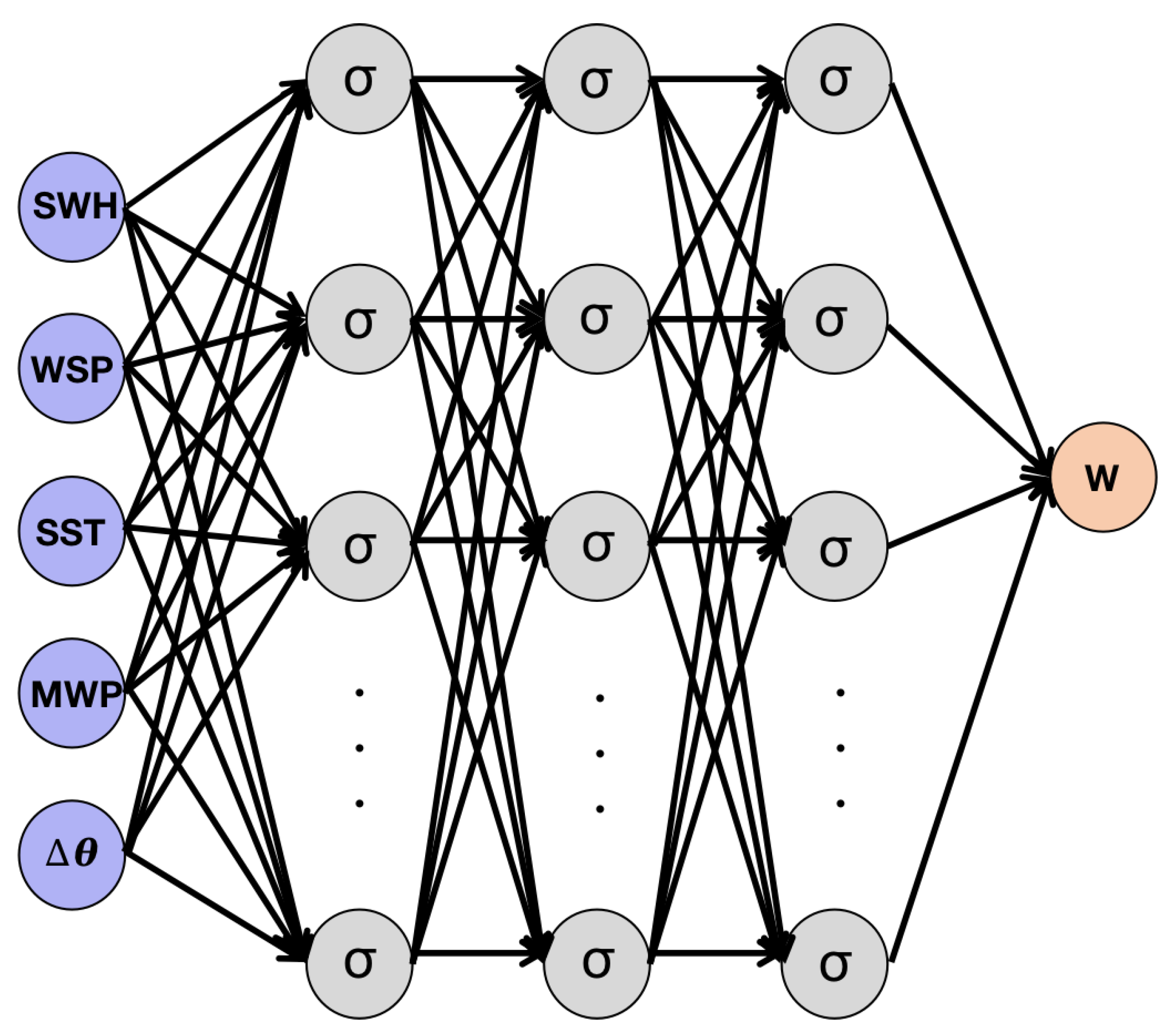
Figure 2 shows the structure of the whitecap fraction parameterization based on the DNN, which has a 5-layer structure, including an input layer, an output layer, and three hidden layers. The number of neurons in the three hidden layers is 16, 8, and 4. To better learn the nonlinear variation of whitecaps, the rectified linear unit [30] is used as the activation function of each neuron. Therefore, it can be regarded as constructing a new function W ( S W H ,   W S P ,   S S T ,   M W P ,   Δ θ ) through DNN to obtain the W value, the inputs are SWH, WSP, SST, MWP, and Δ θ , the output is the satellite-derived W data. All of the input data are normalized as shown in Equation (1).
X n o m = X X m i n X m a x X m i n  
where X is the original data, X n o m is the normalized data, X m a x is the maximum value in the dataset, and X m i n is the minimum value in the dataset.
The DNN continuously updates the weights in the hidden layer by calculating the error between the output and the label until the optimal model is obtained, using satellite-derived W data as the label for training and adding early-stopping to prevent the model from overfitting. The ratio of the model training data and validation data is 7:3. The batch size is set to 256, Epoch is set to 100, and the mean solution error is chosen as the loss function during training. Since this study only has one monthly average whitecap mapping for October 2006, the amount of data is not sufficient, and the strict division between training and testing sets will affect the model’s characterization of the global variability of the whitecap, so this study uses the DNN as a fitting method and uses the same dataset as the training and validation datasets. In the evaluation of the validation dataset, the root mean square error (RMSE), mean absolute error (MAE), and coefficient (R) are mainly used, as shown in Equations (2)–(4).
R M S E = 1 N i = 1 N ( W i * W i ) 2
M A E = 1 N i = 1 N | W i * W i |
R = i = 1 N ( W i W ¯ ) ( W i * W * ¯ ) i = 1 N ( W i W ¯ ) 2 · i = 1 N ( W i * W * ¯ ) 2  
where N is the total number of data, i denotes cases, W i is the value of satellite-derived W data, W i * is the W value calculated by the parameterization, W ¯ is the average value of satellite-derived W data, and W * ¯ is the average of the W value calculated by the parameterization.
Figure 3 shows the variation of W with wind speed for the three schemes (Table 1), where the SST in A16 is taken as 10, 20, and 30 °C, respectively. It can be seen that the difference in W between A16 and S13 is not significant even at different SST, and the dependence of A16 on wind is slightly smaller than that of S13. Compared with M80, the W of S13 and A16 are larger at low wind speeds and smaller at high wind speeds.

3. Results

By training the DNN model using variables such as wind speed, significant wave height, and so on, we obtain a new parameterization W ( S W H ,   W S P ,   S S T ,   M W P ,   Δ θ ) for the whitecap fraction (W). In the following, the new scheme is evaluated (Section 3.1) and explained (Section 3.2) in detail using the October 2006 satellite-derived W data.

3.1. Evaluation of W Parameterization

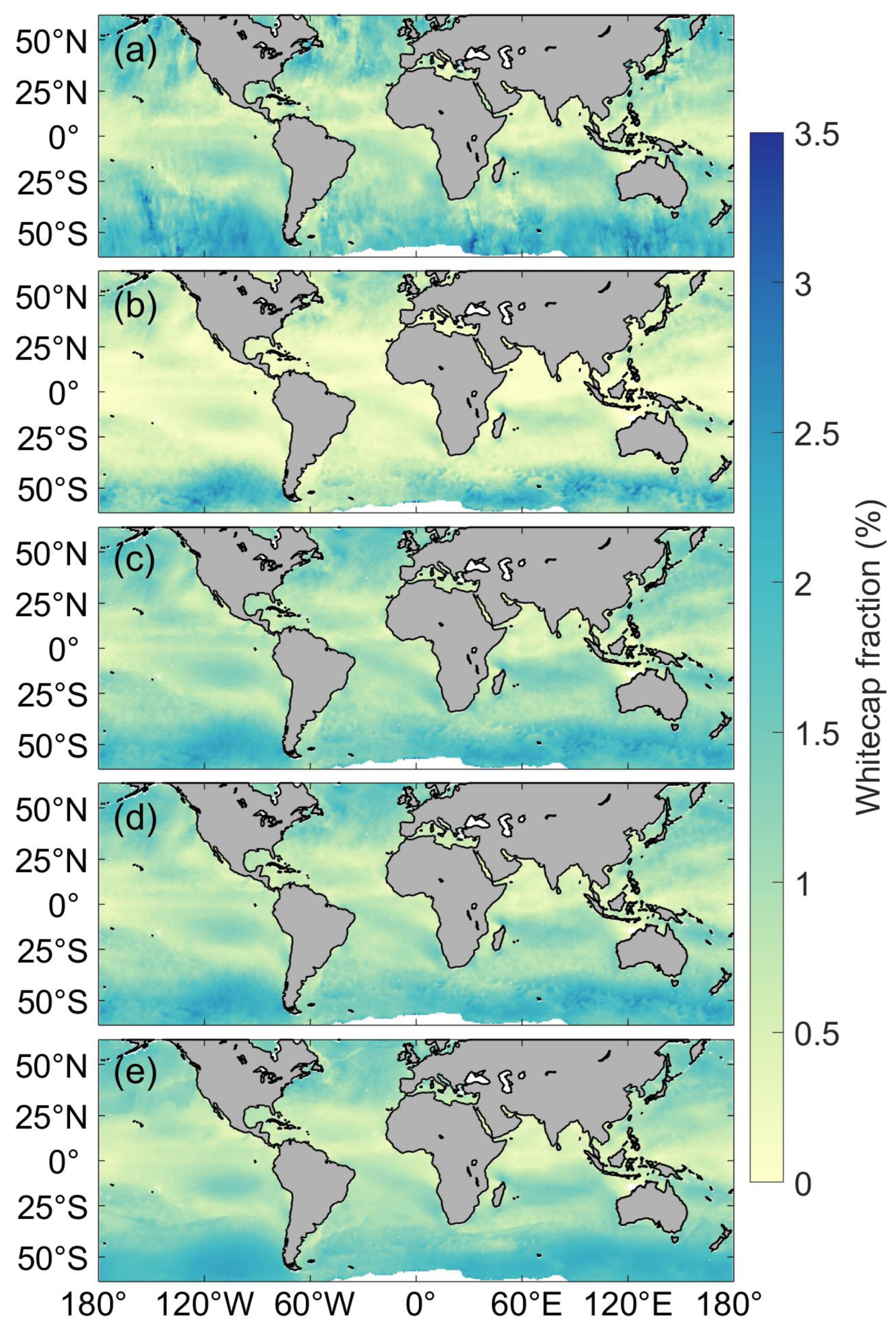
In this first section, the DNN-based W parameterization (NN-W) is evaluated. Figure 4 shows the spatial distribution of the results of different W parameterizations. In general, all of the schemes can portray the spatial distribution of W well, basically consistent in magnitude. The W values calculated by these schemes show a spatial variability with latitude, indicating the high dependence of W on wind speed. Specifically, the W derived from the satellite has an obvious high-value annual distribution band at 50° in the southern hemisphere. By comparing the wind speed field in October 2006, we find that the variation of W cannot be perfectly explained by the modalities of wind speed alone, so it is necessary to add more physical variables to simulate W. The result of M80 is shown in Figure 4b, although this solution can accurately reflect the distribution of the high-value region of W at mid-latitudes, the value of W for low latitudes is significantly lower than that of satellite-based W data, probably due to the relatively low wind speed at low latitudes [15]. The spatial distribution presented by the two parameterization schemes in Figure 4c,d is quite consistent; on one hand, due to the fact that both schemes are developed by fitting the same dataset, and on the other hand, because even though A16 additionally takes into account the effect of sea surface temperature, there are other important factors missing. The results of NN-W show a smoother spatial distribution of W compared to the other schemes, but the underestimation of high values of W may be due to the modulation effect of predictors such as significant wave height and mean wave period, which reduces the high dependence of the model on wind speed to a certain extent.
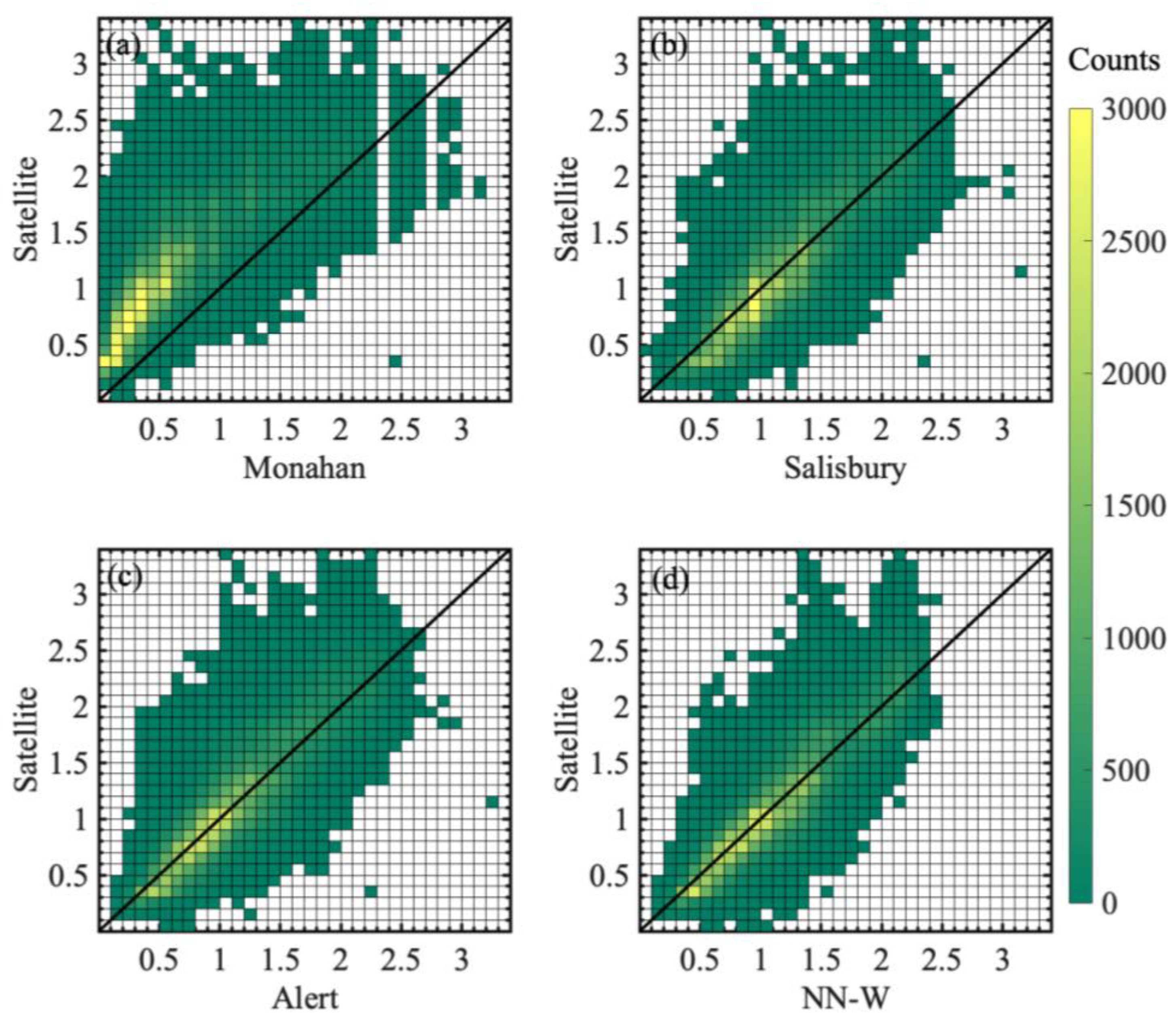
To further illustrate the reliability of NN-W, Figure 5 compares the binscatter plot of NN-W with other parameterizations of W. In Figure 5a, it can be seen that M80 clearly underestimates the value of W when the W value is low (which may correspond to low wind speeds). The difference between S13 and A16 is small, and the scatter distribution is generally symmetrical along the diagonal, while A16 is closer to the diagonal for W values of 0.5–1.5%, indicating that A16 works better, especially at low and medium W values. In comparison, the NN-W produces a more symmetric and concentrated distribution of W along the diagonal with fewer outliers compared to other schemes from low to high W values, indicating that the DNN-based W parameterization has a better representation of W values. This might be related to the fact that the scheme relies on more than just wind speed.
The computational accuracy of the NN-W is evaluated. Table 2 quantifies the accuracy of the four parameterizations using RMSE, MAE, and R. The NN-W produces the best result with a RMSE of only 0.22%, which is 14.6% lower compared to the A16, and the difference between the results of the two schemes statistically passes the t-test with a 95% confidence level. Meanwhile, the NN-W produces the smallest MAE. The R is the spatial correlation of W values, and the change in R values from the four schemes indicates that the NN-W can most accurately capture the spatial variation of the W values.
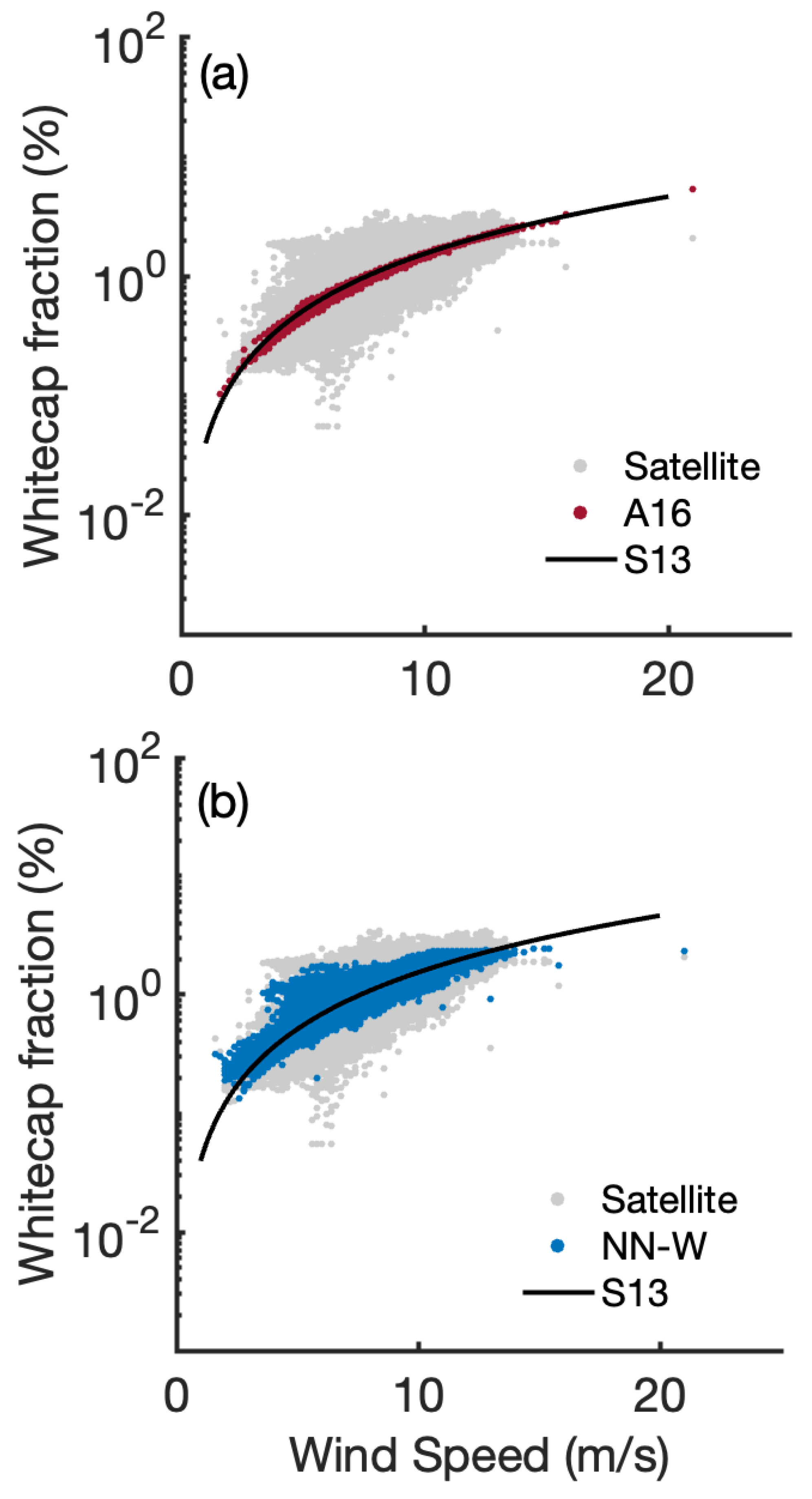
The ability of the NN-W scheme to represent the variability (spread) of W is evaluated as well. Figure 6a,b shows the scatter plots of the calculated W of A16 and NN-W parameterizations against the satellite-based W data, respectively. In general, both schemes reflect the increase in W values with wind speed. Although A16 has some of the variability of W at low and medium wind speeds, the variability becomes insignificant at high wind speeds, which may be related to the fact that only one additional variable, SST, is considered [19]. In contrast, NN-W can better represent the W variability at the same wind speed. This leads to one of the most important conclusions of this study: the W parameterization based on the DNN model can better characterize the variability of satellite-based W data, and the variability shows a trend of increasing and then decreasing with increasing wind speed. In other words, the NN-W can explain the variability of W caused by non-wind speed factors much better than A16, indicating that it is useful to consider multiple factors in the W parameterization to simulate the variability of W. The algorithm for W is still being refined and the latitudinal variation of the satellite W may change in the future, which could lead to a change in W variability [17].

3.2. Understanding of W Parameterization

In this subsection, we will try to interpret the NN-W. Figure 7 shows the bias of W values calculated by the NN-W and the A16. It can be seen that the positive W bias is mainly dominant in the northern hemisphere and in the equatorial region, while in the southern hemisphere, the W bias is alternately positive and negative in all directions. The larger bias of W values in the nearshore may be related to the more complex mechanism of whitecap generation. Anguelova et al. [31] summarized the main factors influencing the spatial variability of W in different regions globally. The SWH and the fetch ( g ( S W H / W S P ) 2 ) explain most of the variability of W at higher latitudes, and the main contribution of SST to variability is concentrated at low latitudes. Comparing to Figure 6 in [31], we find that the positive bias of the W value in Figure 7 is mainly concentrated in the area dominated by the wind, and the negative bias is mainly concentrated in the field dominated by the SWH. This shows that the W parameterization based on the DNN reduces the influence of wind on W in the area dominated by SWH and further enhances the W in the wind-dominated area compared with the A16.
Since sea-salt aerosol production is linearly related to the W, the deviation of W calculated with the NN-W from W calculated with A16 will directly affect the sea-salt aerosol estimation. S13 and A16 will not differ much in the total ocean sea-salt aerosol estimation since both schemes produce a low variability of W (Figure 6a). In contrast, the NN-W parameterization could account for more variability of W (Figure 6b) and tend to reduce the uncertainties in sea-salt aerosol estimation.
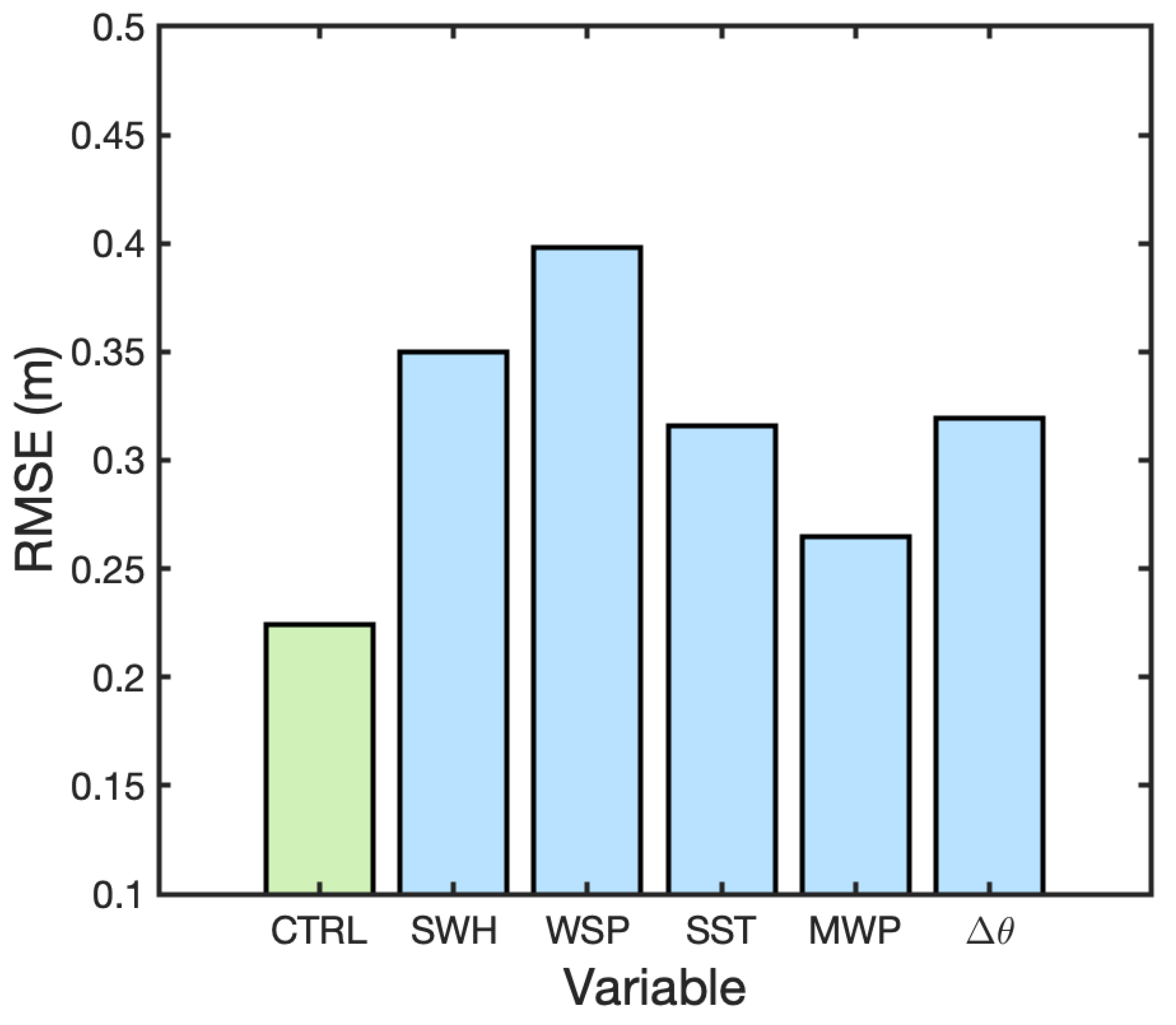
In order to explain the importance of different variables in the W parameterization, a permutation test is performed on the NN-W parameterization, i.e., one of the variables in the input data is randomly disrupted and then input into the DNN for calculation. Here, we use the variation of RMSE to evaluate the importance of different predictors. The greater the change of RMSE, the more important the variable is, since this indicates that the change of that variable has a greater impact on the accuracy. From Figure 8, the importance of the predictor, in descending order, is: WSP, SWH, Δ θ , SST, and MWP. This not only further proves the role of wind speed in the W parameterization, but also shows that SWH is one of the indispensable variables in the W parameterization [15]. Surprisingly, the importance of Δ θ turns out to be nearly equal to that of SST. It is not difficult to understand that a Δ θ of zero (the same wind and wave direction) may make the wave height higher and, thus, produce more whitecaps. This is different from the effects of the deviation of wind and current directions. Winds following currents may decrease W [32]. These main factors, contributing to the spread of W, may also be the main source of uncertainty in sea-salt aerosol estimates. All results here are limited by the use of only one month of W data. If more W data were obtained, we could discuss the main factors influencing the variability of W in different regions from the neural network perspective.

4. Discussion

4.1. Data Selection and Uncertainty

In the course of our study, we found that the uncertainty of the input data affects the accuracy of the W parameterization; for example, there are some differences in the wind speed data from ECMWF and QuikSCAT [15], which can increase the uncertainty of the W parameterization in use. Although the W scheme can be adjusted by correcting the deviation of wind speed from different sources, this is not rigorous. In contrast, the neural network-based W parameterization overcomes this problem well by transfer learning, which makes the NN-W more promising for use. Noticeably, there are two limitations in our parameterization. First, we use the wind speeds from QuikSCAT with maximum wind speeds usually below 24 m/s. Second, the neural network may be inaccurate for forecasting when the inputs are beyond the threshold of the training data. Thus, our model may not necessarily be accurate in some conditions, such as at high wind speed conditions. The parameterization could be further improved with more in situ data.

4.2. Comparison with Classic Machine Learning Methods

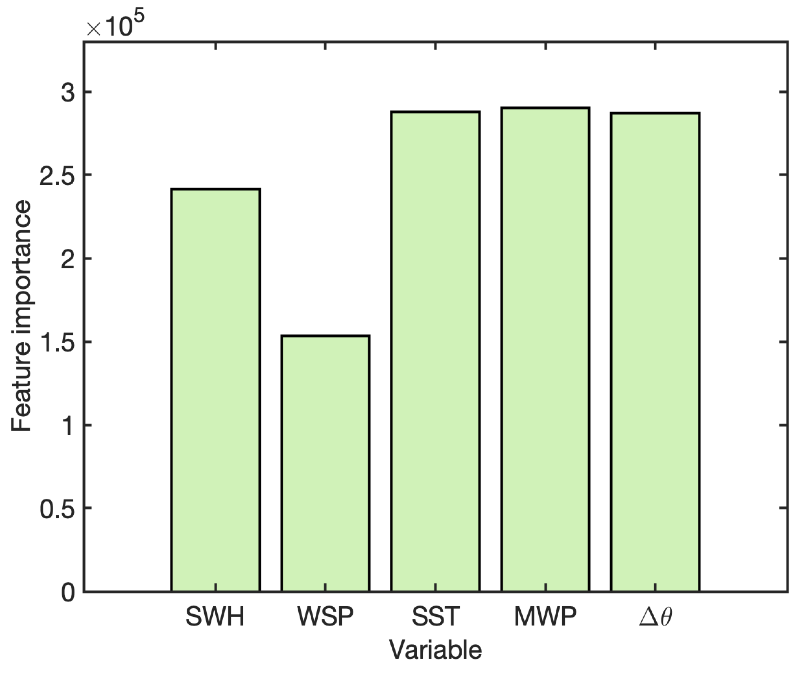
Besides the DNN, classic machine learning methods may also obtain valuable parameterization, such as the Light Gradient Boosting Machine (LightGBM). From the experiment based on the LightGBM (Lgb-W), the RMSE, MAE, and R of the W are 0.15, 0.11, and 0.96, respectively. The results of Lgb-W seem to be better than NN-W. When we analyze the feature importance of variables (see Figure 9), however, it is found that the importance of the features is unexpected. In the Lgb-W, the wind speed is the least important factor and the mean wave period is the most important one. This is clearly incorrect. As the focus of this study is on how to use a neural network to characterize the variability of W and interpret it in a reasonable way, from this perspective, NN-W is more appropriate and has more potential to be used for W estimates.

4.3. Adding Physical Constraints to the Model

As the application of artificial intelligence in earth system science continues to grow, it has been found that it is difficult to make further breakthroughs in forecast accuracy by simply applying a particular algorithm to the forecast or the identification of variables. Even when multiple models are used for forecasting, the improvement is limited [33]. On one hand, neural networks are like a black box with no insight into their internal mechanisms, and direct use of existing models for forecasting may lead to mass or energy non-conservation; on the other hand, forecasting results without physical constraints may run counter to physical cognition. To solve these problems, attempts have been made to add some known physical formulas or laws as constraints in neural networks [34,35]. Previously, the simultaneous observations in the W observation dataset had only a few variables and a small amount of data. This posed difficulties in developing multivariate W parameterizations using in-situ observation datasets directly. However, those W parameterization schemes were developed based on observational data, and while available, they are not globally applicable and have only regional representativeness. Still, their incorporation into the NN-W parameterization may improve regional simulation accuracy. In this paper, we tried to add some widely used W parameterization as physical constraints, such as M80, during the model’s training, but only obtained worse results. We consider the following two main reasons for this situation. First, although M80 is a widely used W parameterization, it still has limitations, especially in the inversion of satellite-derived W data where the effect is worse than that of a single NN-W. Secondly, the current W parameterization is still dominated by the empirical function of wind speed, which cannot be considered as the real physical formulation of W. Therefore, when using a physic-informed neural network for parameterization research, more universal physical formulas should be chosen and fewer empirical physical formulas should be used to bring out the real effect of a physic-informed neural network.

5. Conclusions

The purpose of this study was to develop a new multivariate W parameterization using DNN to better characterize the variability of W due to various factors and to interpret it in some way from a neural network perspective. The NN-W uses SWH, WSP, SST, MWP, and Δ θ as inputs, and the satellite-derived W data as labels for training, resulting in a new intelligent W ( S W H ,   W S P ,   S S T ,   M W P ,   Δ θ ) parameterization. This scheme not only outperforms A16 in the accuracy of W values calculation and can reduce the RMSE of W values by 15%, but also better explains the variability of W. Compared with A16, the new W parameterization clearly reflects the effect of significant wave height on W. However, the addition of multiple factors makes W parameterization less dependent on wind speed, which may be the reason for lower W values by NN-W. The importance of different input variables in the neural network is ranked by permutation test, and the importance is ranked from largest to smallest: WSP, SWH, Δ θ , SST, and MWP. This further deepens the understanding of W and is extremely informative for modeling the physical parameterization of W.
The improved description of W variability by NN-W is expected to better explain the uncertainties in the parameterization of sea-salt aerosol fluxes as well as calculate air-sea momentum flux. Besides, W also influences the calculation of air-sea heat fluxes, since the generation of sea spray is sensitive to W [36]. Our future work will focus on combining different parameterizations with satellite-derived data to develop a multivariate global W parameterization, and on assessing the impact of NN-W on the uncertainty of sea-salt aerosol flux parameterizations.

Author Contributions

Conceptualization, S.Z. and F.X.; methodology, S.Z.; software, S.Z. and R.S.; validation, S.Z., F.X. and R.S.; data curation, S.Z.; writing—original draft preparation, S.Z.; writing—review and editing, S.Z., F.X. and R.S.; visualization, S.Z.; supervision, F.X.; funding acquisition, F.X. All authors have read and agreed to the published version of the manuscript.

Funding

This research was funded by the National Key Research and Development Program of China, grant number 2021YFC3101601 and the National Natural Science Foundation of China, grand number 42176019.

Data Availability Statement

QuikSCAT data are produced by Remote Sensing Systems and sponsored by the NASA Ocean Vector Winds Science Team (www.remss.com, accessed on 30 September 2022). Reanalysis data can be acquired at the Climate Data Store (https://cds.climate.copernicus.eu, accessed on 30 September 2022).

Acknowledgments

The authors thank the ECMWF and NCAR for providing the reanalysis and satellite data used in this paper. Special thanks to Haili Wang for providing W data selflessly, and to Fubin Li for his helpful suggestions.

Conflicts of Interest

The authors declare no conflict of interest.

References

  1. Anguelova, M.D.; Webster, F. Whitecap Coverage from Satellite Measurements: A First Step toward Modeling the Variability of Oceanic Whitecaps. J. Geophys. Res. Atmos. 2006, 111, C03–C017. [Google Scholar] [CrossRef] [Green Version]
  2. Monahan, E.C.; Muircheartaigh, I. Optimal Power-Law Description of Oceanic Whitecap Coverage Dependence on Wind Speed. J. Phys. Oceanogr. 1980, 10, 2094–2099. [Google Scholar] [CrossRef]
  3. Bortkovskii, R.S.; Novak, V.A. Statistical Dependencies of Sea State Characteristics on Water Temperature and Wind-Wave Age-ScienceDirect. J. Mar. Syst. 1993, 4, 161–169. [Google Scholar] [CrossRef]
  4. Bortkovskii, R.S. Water-Temperature Effect on the Spectral Density of Wind Gravity Waves and on Sea-Surface Roughness. Izv. Atmos. Ocean. Phys. 2012, 48, 193–199. [Google Scholar] [CrossRef]
  5. Sugihara, Y.; Tsumori, H.; Ohga, T.; Yoshioka, H.; Serizawa, S. Variation of Whitecap Coverage with Wave-Field Conditions. J. Mar. Syst. 2007, 66, 47–60. [Google Scholar] [CrossRef]
  6. Zhao, D.; Toba, Y. Dependence of Whitecap Coverage on Wind and Wind-Wave Properties. J. Oceanogr. 2001, 57, 603–616. [Google Scholar] [CrossRef]
  7. Brumer, S.E.; Zappa, C.J.; Brooks, I.M.; Tamura, H.; Brown, S.M.; Blomquist, B.W.; Fairall, C.W.; Cifuentes-Lorenzen, A. Whitecap Coverage Dependence on Wind and Wave Statistics as Observed during SO GasEx and HiWinGS. J. Phys. Oceanogr. 2017, 47, 2211–2235. [Google Scholar] [CrossRef]
  8. Blanchard, D.C. The Electrification of the Atmosphere by Particles from Bubbles in the Sea. Prog. Oceanogr. 1963, 1, 73–202. [Google Scholar] [CrossRef]
  9. Blanchard, D.C. The Production, Distribution, and Bacterial Enrichment of the Sea-Salt Aerosol. In Air-Sea Exchange of Gases and Particles; Springer: Berlin/Heidelberg, Germany, 1983; pp. 407–454. [Google Scholar]
  10. Thorpe, S. Bubble Clouds and the Dynamics of the Upper Ocean. Q. J. R. Meteorol. Soc. 1992, 118, 1–22. [Google Scholar] [CrossRef]
  11. Andreas, E.L.; Mahrt, L.; Vickers, D. An Improved Bulk Air–Sea Surface Flux Algorithm, Including Spray-mediated Transfer. Q. J. R. Meteorol. Soc. 2015, 141, 642–654. [Google Scholar] [CrossRef]
  12. Monahan, E.C.; Fairall, C.W.; Davidson, K.L.; Boyle, P.J. Observed Inter-Relations between 10m Winds, Ocean Whitecaps and Marine Aerosols. Q. J. R. Meteorol. Soc. 1983, 109, 379–392. [Google Scholar] [CrossRef]
  13. Wang, H.; Yang, Y.; Dong, C.; Su, T.; Sun, B.; Zou, B. Validation of an Improved Statistical Theory for Sea Surface Whitecap Coverage Using Satellite Remote Sensing Data. Sensors 2018, 18, 3306. [Google Scholar] [CrossRef] [Green Version]
  14. Monahan, E.; Spiel, D.; Davidson, K. A Model of Marine Aerosol Generation via Whitecaps and Wave Disruption. In Oceanic Whitecaps; Springer: Berlin/Heidelberg, Germany, 1986; pp. 167–174. [Google Scholar]
  15. Salisbury, D.J.; Anguelova, M.D.; Brooks, I.M. On the Variability of Whitecap Fraction Using Satellite-Based Observations. J. Geophys. Res. Ocean. 2013, 118, 6201–6222. [Google Scholar] [CrossRef] [Green Version]
  16. Anguelova, M.D.; Bettenhausen, M.H.; Johnston, W.F.; Gaiser, P.W. Passive Remote Sensing of Oceanic Whitecaps: Updated Geophysical Model Function. In Proceedings of the 2017 IEEE International Geoscience and Remote Sensing Symposium (IGARSS), Fort Worth, TX, USA, 23–28 July 2017. [Google Scholar]
  17. Anguelova, M.D.; Bettenhausen, M.H. Whitecap Fraction From Satellite Measurements: Algorithm Description. J. Geophys. Res. Ocean. 2019, 124, 1827–1857. [Google Scholar] [CrossRef]
  18. Goddijn-Murphy, L.; Woolf, D.K.; Callaghan, A.H. Parameterizations and Algorithms for Oceanic Whitecap Coverage. J. Phys. Oceanogr. 2011, 41, 742–756. [Google Scholar] [CrossRef]
  19. Albert, M.F.; Anguelova, M.D.; Manders, A.; Schaap, M.; de Leeuw, G. Parameterization of Oceanic Whitecap Fraction Based on Satellite Observations. Atmos. Chem. Phys. 2016, 16, 13725–13751. [Google Scholar] [CrossRef] [Green Version]
  20. Rémy, S.; Anguelova, M.D. Improving the Representation of Whitecap Fraction and Sea Salt Aerosol Emissions in the ECMWF IFS-AER. Remote Sens. 2021, 13, 4856. [Google Scholar] [CrossRef]
  21. Zhou, S.; Xie, W.; Lu, Y.; Wang, Y.; Zhou, Y.; Hui, N.; Dong, C. ConvLSTM-Based Wave Forecasts in the South and East China Seas. Front. Mar. Sci. 2021, 8, 740. [Google Scholar] [CrossRef]
  22. Bethel, B.J.; Dong, C.; Zhou, S.; Cao, Y. Bidirectional Modeling of Surface Winds and Significant Wave Heights in the Caribbean Sea. J. Mar. Sci. Eng. 2021, 9, 547. [Google Scholar] [CrossRef]
  23. Zheng, G.; Li, X.; Zhang, R.-H.; Liu, B. Purely Satellite Data–Driven Deep Learning Forecast of Complicated Tropical Instability Waves. Sci. Adv. 2020, 6, eaba1482. [Google Scholar] [CrossRef]
  24. Xu, G.; Cheng, C.; Yang, W.; Xie, W.; Kong, L.; Hang, R.; Ma, F.; Dong, C.; Yang, J. Oceanic Eddy Identification Using an AI Scheme. Remote Sens. 2019, 11, 1349. [Google Scholar] [CrossRef] [Green Version]
  25. Bolton, T.; Zanna, L. Applications of Deep Learning to Ocean Data Inference and Subgrid Parameterization. J. Adv. Model. Earth Syst. 2019, 11, 376–399. [Google Scholar] [CrossRef] [Green Version]
  26. Zanna, L.; Bolton, T. Data-Driven Equation Discovery of Ocean Mesoscale Closures. Geophys. Res. Lett. 2020, 47, e2020GL088376. [Google Scholar] [CrossRef]
  27. Han, G.; Cen, H.; Jiang, J.; Gao, X.; Jiang, X.; Zhou, S.; Xie, W.; Ji, J.; Bethel, B.J.; Dong, C. Applying Machine Learning in Devising a Parsimonious Ocean Mixing Parameterization Scheme. Deep Sea Res. Part II Top. Stud. Oceanogr. 2022, 203, 105163. [Google Scholar] [CrossRef]
  28. Liang, J.-H.; Yuan, J.; Wan, X.; Liu, J.; Liu, B.; Jang, H.; Tyagi, M. Exploring the Use of Machine Learning to Parameterize Vertical Mixing in the Ocean Surface Boundary Layer. Ocean Model. 2022, 176, 102059. [Google Scholar] [CrossRef]
  29. Hersbach, H.; Bell, B.; Berrisford, P.; Biavati, G.; Horányi, A.; Muñoz Sabater, J.; Nicolas, J.; Peubey, C.; Radu, R.; Rozum, I.; et al. ERA5 Monthly Averaged Data on Single Levels from 1979 to Present. Copernic. Clim. Change Serv. (C3S) Clim. Data Store (CDS) 2019, 10, 252–266. [Google Scholar]
  30. Nair, V.; Hinton, G.E. Rectified Linear Units Improve Restricted Boltzmann Machines. In Proceedings of the 27th International Conference on Machine Learning, Haifa, Israel, 21–24 June 2010. [Google Scholar]
  31. Anguelova, M.D.; Bettenhausen, M.H.; Johnston, W.F.; Gaiser, P.W. First Extensive Whitecap Database and Its Use to Study Whitecap Fraction Variability. 2010. Available online: http://ams.confex.com/ams/pdfpapers/174036.pdf (accessed on 17 October 2016).
  32. Liu, M.; Yang, B.; Jia, N.; Zou, Z. Dependence of Estimating Whitecap Coverage on Currents and Swells. J. Ocean Univ. China 2021, 20, 512–520. [Google Scholar] [CrossRef]
  33. Zhou, S.; Bethel, B.J.; Sun, W.; Zhao, Y.; Xie, W.; Dong, C. Improving Significant Wave Height Forecasts Using a Joint Empirical Mode Decomposition–Long Short-Term Memory Network. J. Mar. Sci. Eng. 2021, 9, 744. [Google Scholar] [CrossRef]
  34. Thilges, K.; Plumley, M.; Summers, J.E.; Arbic, B.K.; Buijsman, M. Physics-Informed Neural Networks for Predicting Ocean Spatio-Temporal Fields. J. Acoust. Soc. Am. 2021, 150, A25. [Google Scholar] [CrossRef]
  35. Amini, D.; Haghighat, E.; Juanes, R. Physics-Informed Neural Network Solution of Thermo-Hydro-Mechanical (THM) Processes in Porous Media. arXiv 2022, arXiv:2203.01514. [Google Scholar]
  36. Garg, N.; Ng, E.Y.K.; Narasimalu, S. The Effects of Sea Spray and Atmosphere–Wave Coupling on Air–Sea Exchange during a Tropical Cyclone. Atmos. Chem. Phys. 2018, 18, 6001–6021. [Google Scholar] [CrossRef]
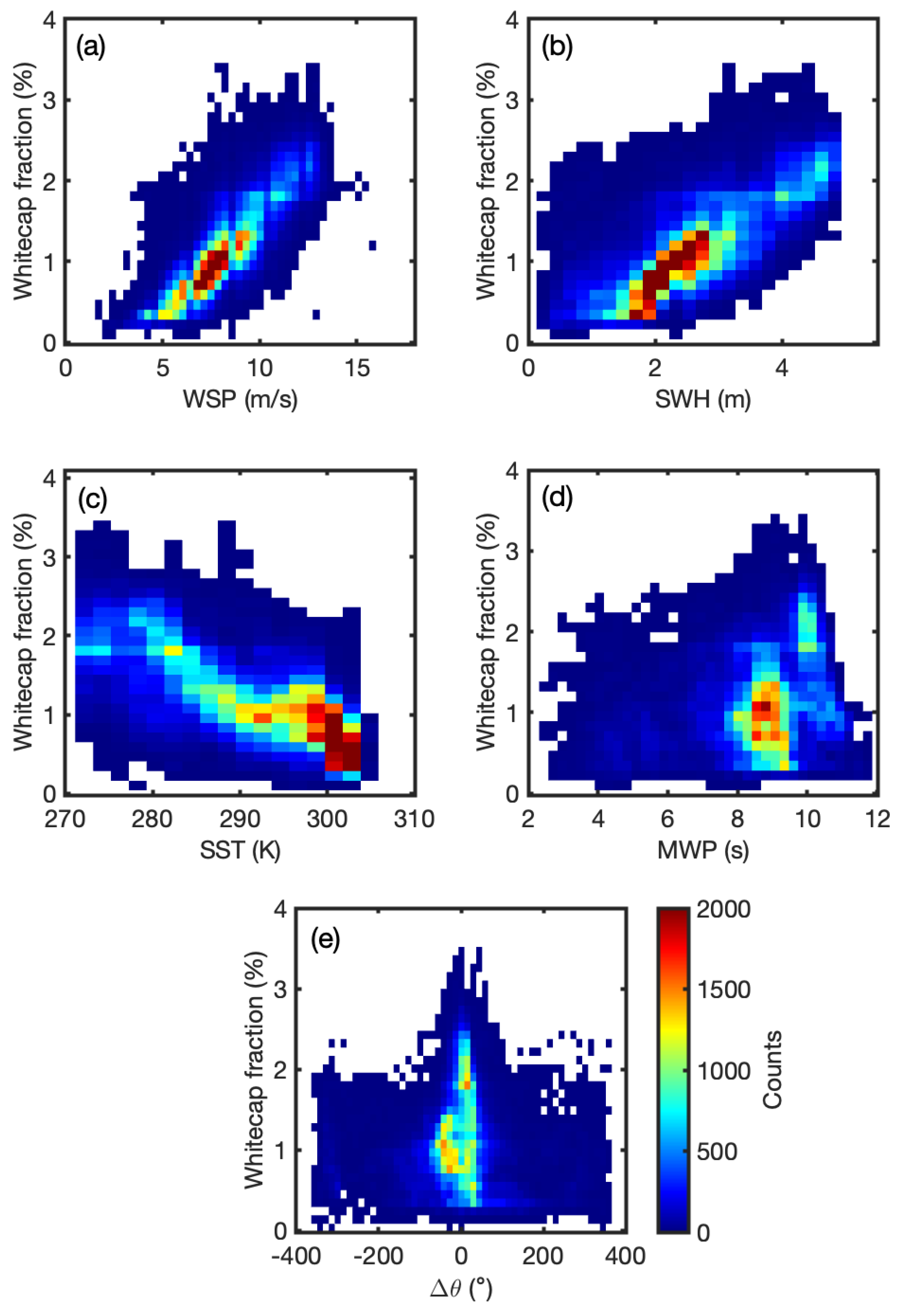
Figure 1. Binscatter plots of whitecap fraction (W) with different variables; (a) the wind speed from QuikSCAT (WSP); (b) significant wave height (SWH); (c) sea surface temperature (SST); (d) mean wave period (MWP); (e) deviation of wind direction from wave direction ( Δ θ ).
Remotesensing 15 00241 g001
Figure 2. Structure of DNN-based whitecap fraction (W) parameterization, σ is the neuron in the hidden layer.
Remotesensing 15 00241 g002
Figure 3. Different parameterizations for whitecap fraction relationships, where the sea surface temperatures in A16 are 10, 20, and 30 °C, respectively.
Remotesensing 15 00241 g003
Figure 4. Monthly average whitecap fraction in October 2006; (a) satellite-derived; (b) M80; (c) S13; (d) A16; (e) NN-W.
Remotesensing 15 00241 g004
Figure 5. Binscatter plots of satellite-derived W data with W values calculated by different parameterizations; (a) M80; (b) S13; (c) A16; (d) NN-W.
Remotesensing 15 00241 g005
Figure 6. Satellite-derived W data for October 2006 at 37 GHz (gray symbols) compared to W values calculated from (a) A16 (red symbols) and (b) NN-W (blue symbols).
Remotesensing 15 00241 g006
Figure 7. The bias of W values calculated by thee NN-W and A16 in October 2006.
Remotesensing 15 00241 g007
Figure 8. The RMSE for different variables in the permutation test. The CTRL is the initial RMSE without permutation test (green bar); the others are the RMSE of permutation tests on different variables (blue bar).
Remotesensing 15 00241 g008
Figure 9. The feature importance for different variables in Lgb-W.
Remotesensing 15 00241 g009
Table 2. Evaluation of the RMSE, MAE, and R metric in different parameterizations.
M80S13A16NN-W
RMSE (%)0.530.270.260.22
MAE (%)0.500.200.190.16
R0.830.860.870.91
Disclaimer/Publisher’s Note: The statements, opinions and data contained in all publications are solely those of the individual author(s) and contributor(s) and not of MDPI and/or the editor(s). MDPI and/or the editor(s) disclaim responsibility for any injury to people or property resulting from any ideas, methods, instructions or products referred to in the content.