Low-Cost IMU and Odometer Tightly Augmented PPP-B2b-Based Inter-Satellite Differenced PPP in Urban Environments

Abstract

Since 23 June 2020, BDS-3 has been entirely operated and obtained the ability of global PNT (Positioning, Navigation, and Timing) services. Afterward, real-time Precise Point Positioning (PPP) service is available in China’s surrounding areas via BDS-3 PPP-B2b signal. However, such a real-time PPP service cannot maintain the high accuracy and continuity of positioning solutions in challenging environments, such as urban environments. For that, we carried out a model by integrating between-satellite single-differenced (BSSD) PPP, a low-cost Inertial Navigation System (INS), and an odometer via an extended Kalman filter. The performance of this integration model was assessed with vehicle-borne data. Results demonstrated that (1) the position RMS (Root Mean Square) of BSSD PPP are 64.33 cm, 53.47 cm, and 154.11 cm. Compared with BSSD PPP, about 31.2%, 23.3%, and 27.3% position improvements can be achieved by using INS. Further enhancements of position RMS benefiting from the odometer are 1.34%, 1.41%, and 1.73% in the three directions. (2) Anyway, the accuracy of BSSD PPP/INS/Odometer tightly coupled integration is slightly higher than that of undifferenced PPP/INS/Odometer integration, with average improvement percentages of 7.71%, 3.09%, and 0.27%. Meanwhile, the performance of BSSD PPP/INS/Odometer integration during the periods with satellite outages is better than the undifferenced PPP-based solutions. (3) The improvements in attitudes from an odometer are more significant on heading angle than the other two attitudes, with percentages of 25.00%. (4) During frequent GNSS outage periods, the reduction in average maximum position drifts provided by INS are 18.01%, 8.95%, and 20.74%. After integrating with an odometer, the drifts can be furtherly decreased by 25.11%, 15.96%, and 20.69%. For attitude, about 41.67% reduction in average maximum drifts of heading angles is obtained.

1. Introduction

China began to build BeiDou Navigation Satellite System (BDS) at the end of the 20th century according to the three-step development strategies [1]. As planned, the first-generation BDS (BDS-1), the second-generation BDS (BDS-2), and the third-generation BDS (BDS-3) were completed successively in 2003, 2012, and 2020, with the corresponding satellite constellations of 3 Geostationary Orbit (GEO) satellites, 5 GEO satellites+5 IGSO (Inclined Geosynchronous Orbit) satellites+4 MEO (Medium Earth Orbit) satellites, and 3 GEO+3 IGSO+24 MEO satellites, respectively. Currently, the global Positioning, Navigation, and Timing (PNT) services of BDS are supported by signals on frequencies B1I (1561.098 MHz), B2I (1207.14 MHz), B3I (1268.52 MHz), B1C (1575.42 MHz), B2a (1176.45 MHz), and B2b (1207.14 MHz) [2,3,4,5,6,7]. Among these services, the Precise Point Positioning (PPP)-B2b enhancement service is of great significance, and also it is considered to be the core support for smart city development in China.

PPP, which was proposed by Zumberger et al. [8] in 1997, is the favored technology for high-accuracy positioning applications. The corresponding model was furtherly developed in the works [8,9,10]. PPP can provide an accurate positioning solution using only a single GNSS receiver by utilizing precise satellite products with about two weeks delay [11,12,13]. Consequently, PPP is mainly for applications in post-processing currently [14,15]. To satisfy the demands of real-time PPP, BDS-3 transmits the orbit/clock corrections of broadcast ephemeris by B2b signal [16,17,18,19]. Multi-GNSS Experiment (MGEX)/iGMAS stations were adopted in [17] to verify the real-time PPP positioning performance using PPP-B2b service in static and simulated-kinematic modes by comparing with the solutions based on Geodetic Benchmark (GBM) final products. It is shown that the positioning performance of real-time PPP is slightly worse than the post-processing PPP in general, according to the statistical results. However, the convergence time of real-time PPP is slightly shorter for the BDS-only in a static model. Tao et al. [16] compared PPP-B2b service with Real-Time Service (RTS) provided by Centre National d’Etudes Spatiales (CNES). Based on the analysis from six stations distributed in China, the positioning accuracy of BDS-3-only PPP with PPP-B2b service in kinematic mode can achieve decimeter-level positioning results, which is consistent with the accuracy of GPS PPP using products of CNES.

However, such a PPP-B2b service-based PPP cannot maintain positioning accuracy and continuity in urban environments [20,21], such as under bridges or trees, etc. In order to overcome the shortcomings of PPP in those circumstances, an Inertial Navigation System (INS) is integrated. INS is capable of providing position, velocity, and attitude results by using measurements from Inertial Measurement Units (IMU) without external observations. However, the position errors of INS will accumulate rapidly over time [22,23]. Meanwhile, integrating PPP and INS can estimate and compensate IMU errors to restrain the divergence [20,22,24]. According to previous works, more reliable position results can be obtained by PPP/INS [20,21,25,26,27,28,29].

Le et al. [25] investigated the Loosely Coupled Integration (LCI) of Single Frequency (SF) PPP/INS, which was validated by a flight experiment. Results showed that the SF-PPP-only positioning performance is visibly improved in the horizontal and vertical components. LCI mode cannot work when there are not enough GNSS observations. Martell in [26] further applied the Tightly Coupled Integration (TCI) of PPP and INS using different grade IMUs and different cut-off satellite angles. The results showed that reliable results could be obtained even if the number of satellites is less than 4. In [27], TCI was compared with LCI by using a tactical-grade IMU to illustrate the benefits of TCI. The position differences of TCI are within 1.0 m, and such errors of LCI are within 5.0 m. The studies above are mainly based on undifferenced GNSS observations. The Dual Frequency (DF) PPP/INS integration using Single-Difference Between-Satellites (BSSD) GPS observations was applied in [28]. During the simulated outages of 10 s~30 s, the position accuracy of BSSD PPP/INS TCI can be decimeter-level. Such accuracy is higher than those using undifferenced observations. Owing to the evolution of multi-constellation GNSS (multi-GNSS), more available observations can be adopted to enhance the integration performance. Gao et al. [21] developed the multi-constellation (GLONASS, BDS, and GPS) TCI of SF PPP/INS, and it was verified by a set of land-borne experiment data. Results showed that significant positum improvements in terms of accuracy, continuity, and reliability could be obtained by INS aiding. Anyway, the performance of conventional GPS SF-PPP can be improved by utilizing the multi-GNSS observation. The enhancement of multi-GNSS on PPP/INS is also illustrated in [29]. According to the results, the positioning and convergence performance of PPP is enhanced significantly by multi-GNSS and INS. However, such impacts in terms of velocity and attitude are invisible.

Based on the works in [20,21,22,23,24,25,26,27,28,29], continuous solutions with high accuracy can be provided by the PPP/INS integration during GNSS outages. However, the positioning errors of PPP/INS still accumulate rapidly, especially for a low-cost IMU when the GNSS signal seriously deteriorates, even interrupts completely around high buildings or under tunnels [30,31]. Such a circumstance can be facilitated by using the velocity information from an odometer. In [31], GPS + GLONASS DF-PPP was integrated with INS and odometer, and simulated GNSS outages were utilized to evaluate the performance in challenging circumstances. According to the results, the position accuracy was furtherly ameliorated by the odometer.

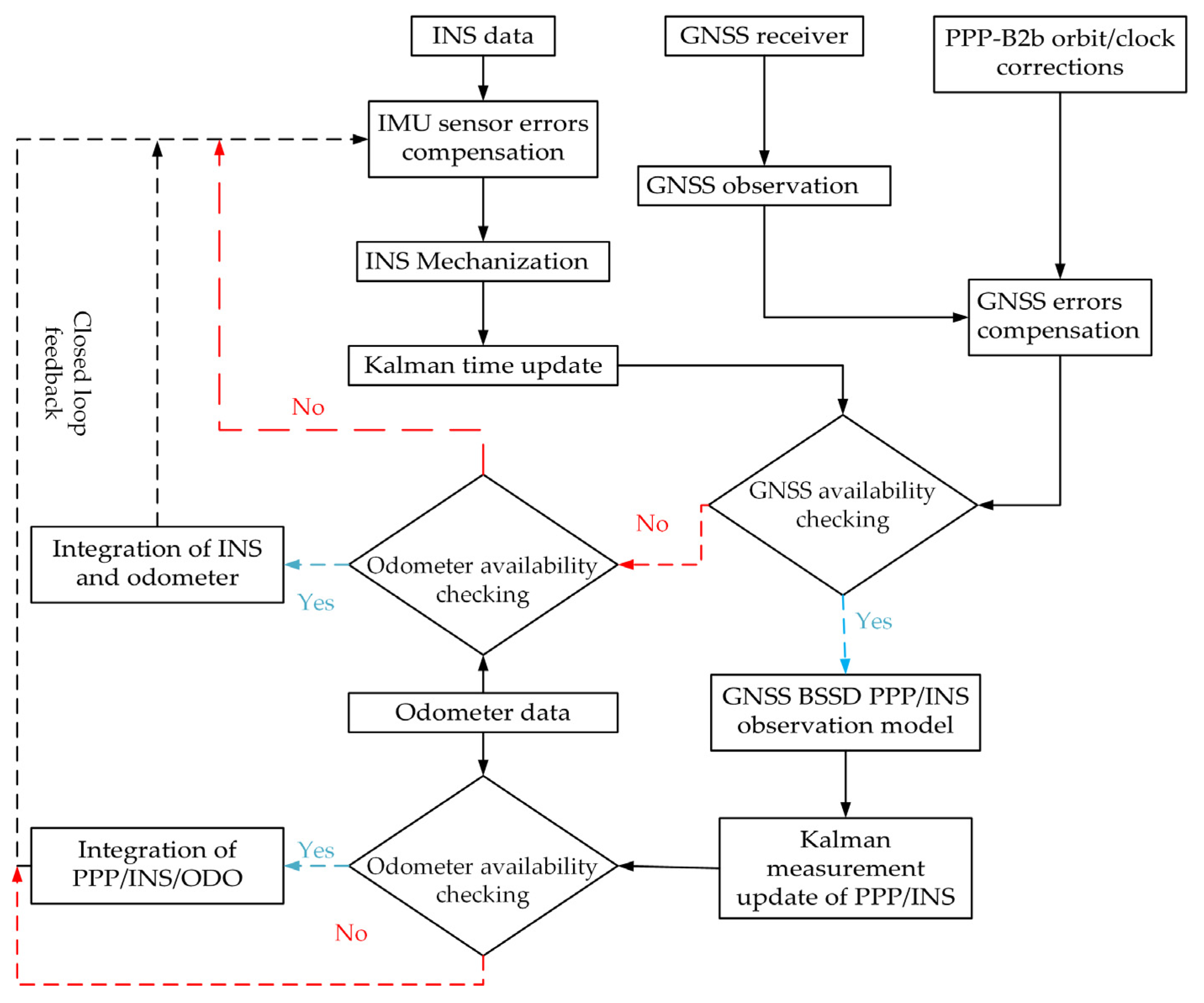
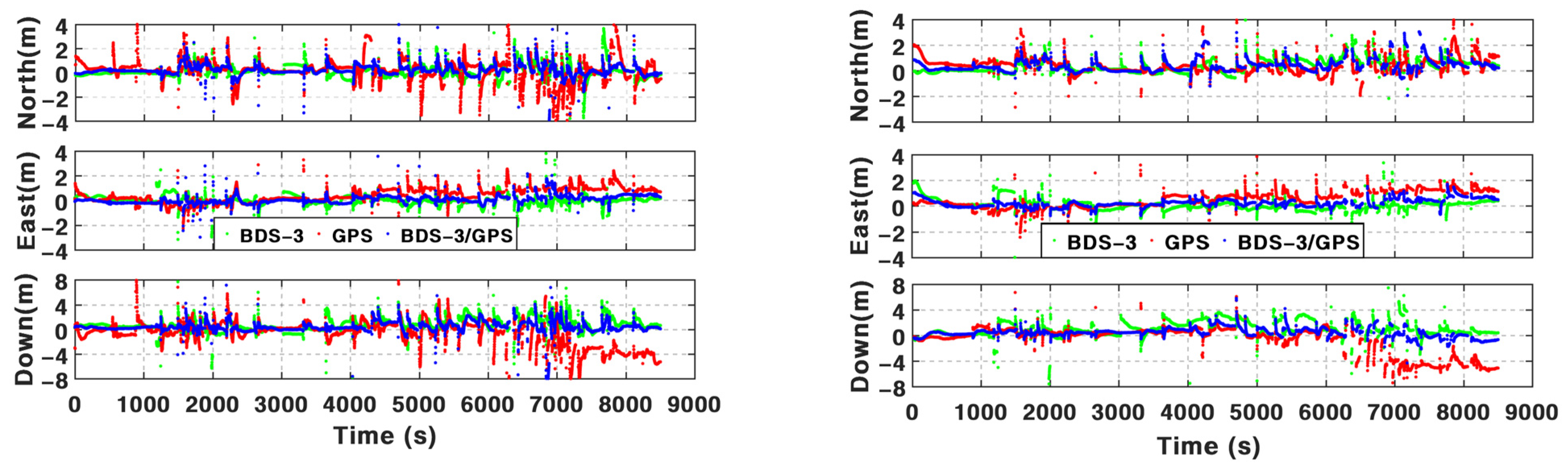
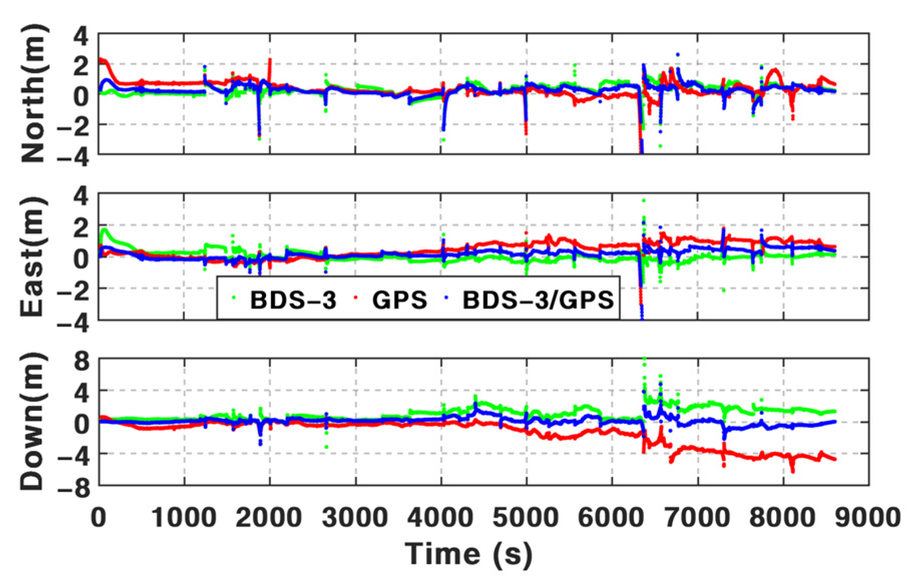
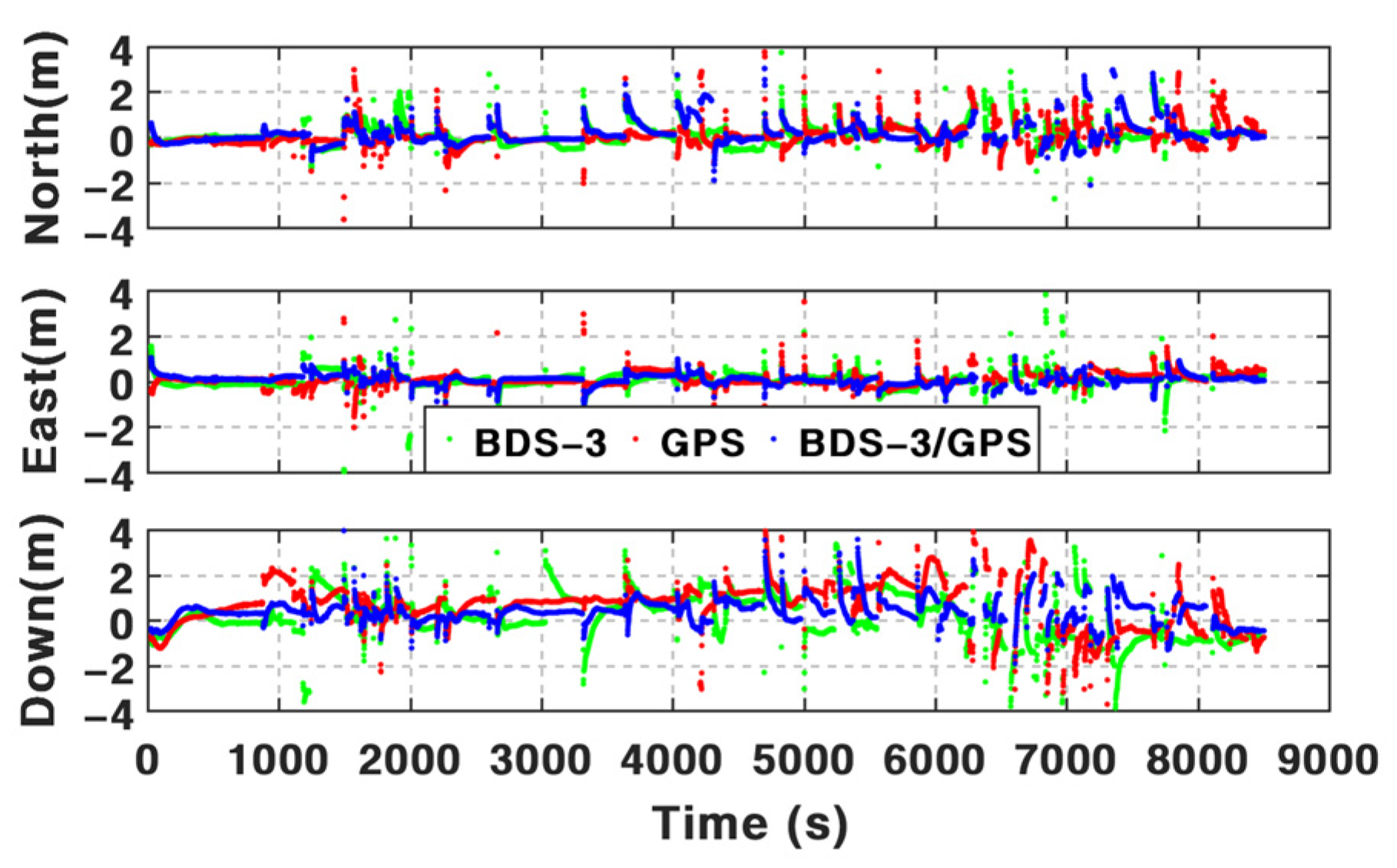
In this paper, we implied PPP/INS/odometer tightly coupled integration model. In comparison with previous works, the contribution of this paper is that such a tightly coupled integration is based on the BSSD model and the BDS-3 PPP-B2b orbit/clock corrections. In order to assess the performance of this algorithm, vehicle-borne data acquired in urban environments are processed and analyzed. The enhancements of a low-cost INS, BSSD BDS-3 PPP model, and an odometer on positioning and attitude determination are discussed in detail.

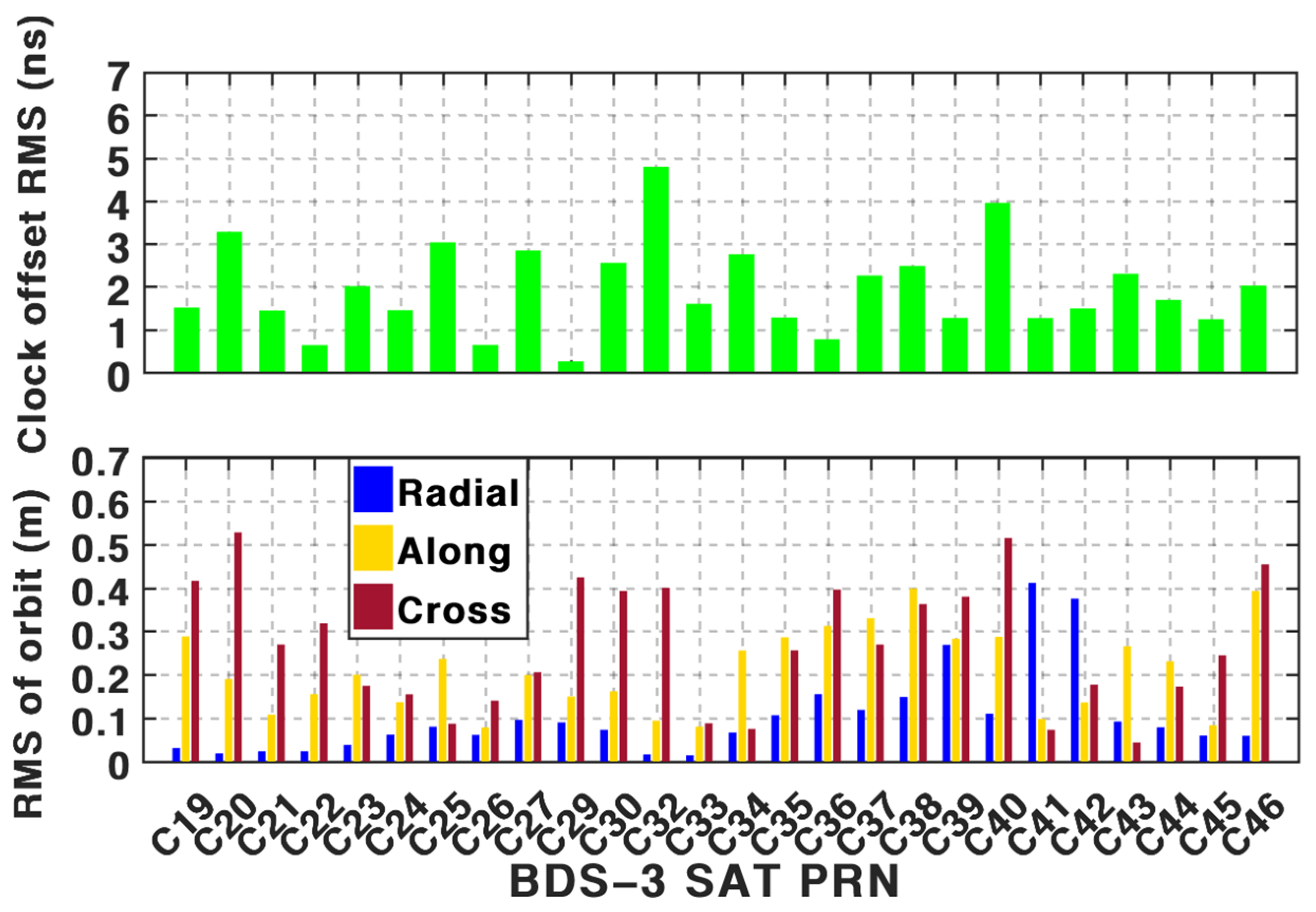
2. Methodology

In this section, the method to recover precise orbit and clock offsets by using the PPP-B2b service is discussed first. Then, the models of PPP/INS TCI and PPP/INS/odometer TCI based on the recovered PPP-B2b orbit/clock offsets and BSSD observation are presented in detail.

2.1. Recovery of Precise Satellite Orbit/Clock with PPP-B2b

The information provided by the PPP-B2b service includes the orbit and satellite clock offset corrections of broadcast products in the satellite-fixed frame (radial, along, and cross directions), which cannot be used directly in positioning. Thus, to apply the corrections in PPP, the precise orbit and clock offsets need to be recovered. The satellite positions computed by broadcast ephemeris are given in the Earth-Centered Earth-Fixed reference (ECEF) frame (e-frame). Therefore, the orbit corrections must be transformed into the ECEF frame by [32]

$$\left[\begin{array}{c}\delta O_x\\ \delta O_y\\ \delta O_z\end{array}\right]=\left[\begin{array}{ccc}{e}_{radial}& e_{along}& e_{cross}\end{array}\right]\left[\begin{array}{c}\delta O_{radial}\\ \delta O_{along}\\ \delta O_{cross}\end{array}\right]$$

(1)

With

$$\left\{\begin{array}{c}{e}_{radial}=r/\left|r\right|\\ e_{cross}=(r\times \dot{r})/\left|r\times \dot{r}\right|\\ e_{along}=e_{radial}\times e_{cross}\end{array}\right.$$

(2)

where ${\left[\begin{array}{ccc}\delta O_{radial}& \delta O_{cross}& \delta O_{along}\end{array}\right]}^T$ is the orbit correction vector in the satellite-fixed frame; ${\left[\begin{array}{ccc}\delta O_x& \delta O_y& \delta O_z\end{array}\right]}^T$ represents the orbit correction vector in the e-frame; $r$ is the satellite position vector and $\dot{r}$ represents the satellite velocity vector, which can be computed by broadcast ephemeris.

By applying the corrections in Equation (1) to broadcast ephemeris, precise satellite positions can be calculated by

$${\left[\begin{array}{c}X\\ Y\\ Z\end{array}\right]}_{prec,B2b}={\left[\begin{array}{c}X\\ Y\\ Z\end{array}\right]}_{brdc}-\left[\begin{array}{c}\delta O_x\\ \delta O_y\\ \delta O_z\end{array}\right]$$

(3)

where ${\left[\begin{array}{ccc}X& Y& Z\end{array}\right]}_{{}_{prec,B2b}}^T$ denotes the vector of precise satellite positions after using the corrections provided by PPP-B2b service; ${\left[\begin{array}{ccc}X& Y& Z\end{array}\right]}_{brdc}^T$ is the vector of satellite positions calculated by broadcast ephemeris.

PPP-B2b service also provides the correction of satellite clock offset. The precise clock offsets can be obtained by

$$d{t}_{prec,B2b}^s=d{t}_{brdc}^s-\frac{C_0}{c}$$

(4)

where $d{t}_{prec,B2b}^s$ is the precise clock offset calculated by using the clock offset derived from broadcast ephemeris ($d{t}_{brdc}^s$) and the PPP-B2b clock correction parameter ($C_0$); $c$ denotes the velocity of light.

2.2. Single-Difference between-Satellites Observational Model

The linearized undifferenced Ionosphere-Free (IF) model of the satellite (k) can be written as

$$P_{{}_{IF}}^k-{\rho }^k-\Delta {\rho }_{P,IF}^k=e_1\delta x_r+e_2\delta y_r+e_3\delta z_r+c{t}_r+m_{wet}\delta d_{wet}+{\epsilon }_{P,IF}$$

(5)

$$L_{{}_{IF}}^k-{\rho }^k-\Delta {\rho }_{L,IF}^k=e_1\delta x_r+e_2\delta y_r+e_3\delta z_r+c{t}_r+m_{wet}\delta d_{wet}-{\lambda }_{IF}{N}_{{}_{IF}}^k+{\epsilon }_{L,IF}$$

(6)

where $P_{IF}^k=\alpha P_1-\beta P_2$ and $L_{IF}^k=\alpha L_1-\beta L_2$ are IF pseudorange and carrier-phase, wherein $\alpha =f_1^2/(f_1^2-f_2^2)$ and $\beta =f_2^2/(f_1^2-f_2^2)$ are IF combination coefficients based on frequencies $f_1$ and $f_2$; $r$ and $k$ represent receiver and satellite; ${\rho }^k$ is the geometric distance between receiver and satellite; $t_r$ represents the receiver clock offset; $m_{wet}$ is the tropospheric wet delay mapping function; $\delta d_{wet}$ is the corrections of zenith wet delay; $E={\left[\begin{array}{ccc}{e}_1^{}& e_2^{}& e_3^{}\end{array}\right]}^T$ is the orientation cosine vector; $\delta p_{GNSS}^e=\left[\begin{array}{ccc}\delta x_r& \delta y_r& \delta z_r\end{array}\right]$ represents receiver position correction in e-frame; ${\lambda }_{IF}$ is the IF wavelength; $N_{IF}^k$ is the IF float ambiguity [13]; $\Delta {\rho }_{L,IF}^k$ and $\Delta {\rho }_{P,IF}^k$ are the errors sum of carrier-phase and pseudorange; ${\epsilon }_{L,IF}$ and ${\epsilon }_{P,IF}$ are the measurement noise of carrier-phase and pseudorange [33].

In addition to the pseudorange and carrier-phase measurements, the Doppler measurements are essential for calculating receiver velocity. The linearized observation equation of Doppler can be expressed as

$$D_{IF}^k-{\dot{\rho }}^k-\Delta {\dot{\rho }}_{D,IF}^k=e_1\delta v_{x,r}+e_2\delta v_{y,r}+e_3\delta v_{z,r}+c{\dot{t}}_r+{\epsilon }_{D,IF}$$

(7)

where $D_{IF}^k=\alpha D_1^k-\beta D_2^k$ is the Doppler measurement in meters; $j$ represents frequency; the dot above the symbol indicates the variation. In general, except for the variation of receiver clocks (${\dot{t}}_r$), satellite clocks, and geometric distance (${\dot{\rho }}^k$), other errors’ variations are close to zero and are ignored. $\delta v_{GNSS}^e=\left[\begin{array}{ccc}\delta v_{x,r}& \delta v_{y,r}& \delta v_{z,r}\end{array}\right]$ are the vector of receiver velocity corrections; $\Delta {\dot{\rho }}_{D,IF}^k$ denotes the sum of Doppler errors; ${\epsilon }_D$ is Doppler noise.

Compared to the undifferenced model, the BSSD model has the advantage that receiver-related errors such as the receiver clock, receiver hardware delay, and unmodelled errors can be eliminated [28,34]. The BSSD IF model can be obtained by

$$\Delta P_{IF}^{km}-\Delta {\rho }^{km}-\Delta {\rho }_{P,IF}^{km}=e_1^{km}\delta x_r+e_2^{km}\delta y_r+e_3^{km}\delta z_r+m_{wet}^{km}\delta d_{wet}+{\epsilon }_{{}_{P,IF}}^{km}$$

(8)

$$\Delta L_{IF}^{km}-\Delta {\rho }^{km}-\Delta {\rho }_{L,IF}^{km}=e_1^{km}\delta x_r+e_2^{km}\delta y_r+e_3^{km}\delta z_r+m_{wet}^{km}\delta d_{wet}-{\mathit{\lambda }}_{IF}^{}\delta {\mathit{N}}_{IF}^{km}+{\epsilon }_{{}_{L,IF}}^{km}$$

(9)

$$\Delta D_{IF}^{km}-\Delta {\dot{\rho }}^{km}-\Delta {\dot{\rho }}_{D,IF}^{km}=e_1^{km}\delta v_{x,r}+e_2^{km}\delta v_{y,r}+e_3^{km}\delta v_{z,r}+{\epsilon }_{{}_{D,IF}}^{km}$$

(10)

where $\Delta L_{IF}^{km}=L_{IF}^m-L_{IF}^k$; $\Delta P_{IF}^{km}=P_{IF}^m-P_{IF}^k$; $\Delta D_{IF}^{km}=D_{IF}^m-D_{IF}^k$; $\Delta {\rho }^{km}={\rho }^m-{\rho }^k$; $\Delta {\dot{\rho }}^{km}={\dot{\rho }}^m-{\dot{\rho }}^k$; $\delta {\mathit{N}}_{IF}^{km}=\delta {\mathit{N}}_{IF}^m-\delta {\mathit{N}}_{IF}^k$; superscripts $k$ and $m$ represent satellite and the reference satellite. In this paper, GPS and BDS separately choose the reference satellite.

2.3. BSSD PPP/INS Tightly Coupled Integration

The innovation vector of TCI is based on the difference between GNSS observations (pseudorange, carrier-phase, and doppler) and the corresponding values predicted by INS [20,21,28]. The state equation and observation equation can be expressed as

$$X_{TCI,k}={\varphi }_{TCI,k,k-1}{X}_{TCI,k-1}+{\mu }_{TCI,k-1},{\mu }_{TCI,k-1}~(0,Q_{TCI,k})$$

(11)

$$Z_{TCI,k}=H_{TCI,k}{X}_{TCI,k}+{\eta }_{TCI,k},{\eta }_{TCI,k}~N(0,R_{TCI})$$

(12)

$$Z_{TCI,k}=\left[\begin{array}{c}{P}_{GNSS,IF}-P_{INS,IF}\\ L_{GNSS,IF}-L_{INS,IF}\\ D_{GNSS,IF}-D_{INS,IF}\end{array}\right]=\left[\begin{array}{c}{Z}_{P_{IF}}\\ Z_{L_{IF}}\\ Z_{D_{IF}}\end{array}\right]$$

(13)

where ${\varphi }_{TCI,k,k-1}$ is the system transform matrix from epoch $k-1$ to epoch $k$; ${\mu }_{TCI,k-1}$ represent the state noise with the covariance of $Q_{TCI,k}$; $Z_{P_{IF}}$, $Z_{L_{IF}}$, and $Z_{D_{IF}}$ represent the innovation vector of pseudorange, carrier-phase, and doppler, respectively; $P_{INS,IF}$, $L_{INS,IF}$, and $D_{INS,IF}$ are the INS-predicted values; $P_{GNSS,IF}$, $L_{GNSS,IF}$, $D_{GNSS,IF}$ are the GNSS measurement; ${\eta }_{TCI,k}$ represents observation noise with the prior covariance of $R_{TCI}$.

In order to obtain the INS-predicted values corresponding to GNSS measurements, the position and velocity of the receiver updated by INS mechanization are required. However, the reference centers of the INS and GNSS antenna are different from each other, which results in a lever-arm system offset. Therefore, the linearization functions $Z_{TCI,k}$ after considering the lever arm can be written as [22,29]

$$\delta Z_{TCI,k}=\left[\begin{array}{c}\delta Z_{P_{IF}}\\ \delta Z_{L_{IF}}\\ \delta Z_{D_{IF}}\end{array}\right]=\left[\begin{array}{c}{C}_1\left(\delta p_{INS}^n+\left(C_b^n{l}^b\times \right)\delta \psi \right)+c\delta t_r-m_{wet}{d}_{wet}\\ C_1\left(\delta p_{INS}^n+\left(C_b^n{l}^b\times \right)\delta \psi \right)+c\delta t_r-m_{wet}{d}_{wet}+\delta N_{IF}{\lambda }_{IF}\\ C_2{D}^{-1}\delta p_{INS}^n+C_n^e{H}_{\psi }\delta \psi +C_n^e\delta v_{INS}^n+C_n^e{C}_b^n\left(l^b\times \right)\delta {\omega }_{ib}^b+c\delta {\dot{t}}_r\end{array}\right]$$

(14)

$$D^{-1}=\left[\begin{array}{ccc}1/(R_M+h)& 0& 0\\ 0& 1/(R_N+h)\cos (B)& 0\\ 0& 0& -1\end{array}\right]$$

(15)

where $\delta Z_{P_{IF}}$, $\delta Z_{L_{IF}}$, and $\delta Z_{D_{IF}}$ represent the differential form of innovation vector; $n$, $b$, and $i$ are the navigation frame (n), the body frame (b), and the inertial frame (i); $C_k^j$ (k = n and b, j = e and n) represent the rotation matrix from the k-frame to the j-frame; $l^b$ is the lever-arm; $\delta p_{INS}^n$, $\delta v_{INS}^n$, and $\delta \psi$ are the corrections of position, velocity, and attitude at IMU center in n-frame; $\delta t_r$ and $\delta {\dot{t}}_r$ represent the corrections of receiver clock offset and drift; $C_1$ is the rotation matrix of position corrections from e-frame to n-frame; $C_2$ is the differential form of $C_n^e$; $\delta {\omega }_{ib}^b$ means gyroscope errors [22,29].

Based on Equation (12), the satellite single-difference matrix (SSDM) can be expressed as [28]

$$SSDM={\left[\begin{array}{cc}SSD{M}_G& 0\\ 0& SSD{M}_B\end{array}\right]}_{3h\times 2m}$$

(16)

$$SSD{M}_B={\left[\begin{array}{cccccccc}1& 0& \cdots & -1& 0& 0& \cdots & 0\\ 0& \ddots & 0& -1& ⋮& ⋮& 0& ⋮\\ ⋮& 0& 1& -1& ⋮& ⋮& ⋮& ⋮\\ ⋮& ⋮& ⋮& ⋮& ⋮& ⋮& ⋮& ⋮\\ ⋮& ⋮& 0& -1& 1& 0& \cdots & ⋮\\ ⋮& ⋮& ⋮& -1& ⋮& \ddots & 0& ⋮\\ ⋮& 0& ⋮& -1& 0& \cdots & 1& 0\\ 0& \cdots & 0& -1& 0& 0& \cdots & 1\end{array}\right]}_{h_2\times m}$$

(17)

where $SSD{M}_G$ is obtained referring to $SSD{M}_B$; $h_1$ and $h_2$ ($h=h_1+h_2$) are the total number of GPS and BDS available satellites; m represents the number of estimated parameters for the BSSD model. BSSD coefficient matrix $H_{BSSD,TCI,k}$ and innovation vector $Z_{BSSD,TCI,k}$ can be calculated by

$$H_{BSSD,TCI,k}=SSDM\times H_{TCI,k}\times SSD{M}^T$$

(18)

$$Z_{BSSD,TCI,k}=SSDM\times Z_{TCI,k}\times SSD{M}^T$$

(19)

$$R_{BSSD,TCI}=SSDM\times R_{TCI}\times SSD{M}^T$$

(20)

In addition, there is Inter-System Bias (ISB) between GPS and BDS [35,36]. To solve this problem, we consider the receiver clock offset of different GNSS as independent parameters and estimate them separately. This method is presented in detail in the works of [37,38]. Anyway, there are two other methods to process ISB [6,36,39]. It is worth mentioning that the receiver clock offset, and drift can be removed in the BSSD PPP/INS TCI model, with the state vector of

$$X_{BSSD,TCI,k}=\left[\begin{array}{ccccccccc}\delta p_{INS}^n& \delta v_{INS}^n& \delta \psi & \delta B_a& \delta B_g& \delta S_a& \delta S_g& \delta d_{wet}& \delta N_{{}_{IF}}^{km}\end{array}\right]$$

(21)

where $\delta p_{INS}^n$, $\delta v_{INS}^n$, and $\delta \psi$ represent the corrections of position, velocity, and attitude; $\delta S_g$ and $\delta B_g$ represent the scale factor and bias of gyroscope; $\delta S_a$ and $\delta B_a$ represent the scale factor and bias of accelerometers [40]; $\delta d_{wet}$ is a wet component of tropospheric zenith delay, and $\delta N_{IF}$ represents ambiguity.

2.4. Odometer-Aided BSSD PPP/INS Tightly-Coupled Integration

In motion scenarios, the vehicle does not slip sideways and upward, which means that the velocity on lateral and vertical will be close to zero and only the forward speed exists [31,32]. Meanwhile, the forward velocity obtained from an odometer can be used as a pseudo-measurement. However, the odometer-measured velocity will be influenced by the scale factor error

$$v_o\approx {\left[\begin{array}{c}{v}_o^v/(1+S_o) 0 0\end{array}\right]}^T$$

(22)

where $v_o^v$ is the forward vehicle velocity measured by the odometer in the vehicle frame (v); $S_o$ represent the scale factor which can be modeled as a random walk process.

The innovation vector of the odometer can be calculated by the difference between the velocity measured by the odometer and predicted by INS predicted one. However, the v-frame and the b-frame are not usually aligned theoretically. Therefore, the innovation vector ($Z_o$) can be described by

$$Z_o=v_o^v-C_b^v{v}_{INS}^b\approx \left[\begin{array}{c}{v}_o^v/(1+S_o)\\ 0\\ 0\end{array}\right]-\left[\begin{array}{c}{v}_{INS}^F\\ v_{INS}^R\\ v_{INS}^D\end{array}\right]+\eta ,\eta ~N(0,{\sigma }_o^2)$$

(23)

where $C_b^v$ denotes the rotation matrix from b-frame to v-frame; $\eta$ is the vector of odometer innovation noise with the prior variance of ${\sigma }_o^2$.

According to Equation (11), $Z_{BSSD,TCI,k}$ can be furtherly expressed as

$$Z_{BSSD,TCI,k}=\left[\begin{array}{c}SSDM\times Z_{TCI,k}\times SSD{M}^T\\ v_o^v-C_b^v{v}_{INS}^b\end{array}\right]$$

(24)

with the linearized form of

$$\delta Z_o=v_{{}_o}^{\mathrm{v}}\delta S_o-C_b^{\mathrm{v}}\left(C_n^b\delta v_{INS}^n-C_n^b\left(v_{INS}^n\times \right)\delta \psi -\left(l_o^b\times \right){\omega }_{ib}^b\delta S_g\right)$$

(25)

where $\delta S_o$ is the correction of the odometer scale factor; $l_o^b$ denotes the lever-arm between the reference center of the odometer and IMU in the b-frame. The corresponding BSSD state vector can be expressed as

$$X_{BSSD,TCI,k}=\left[\begin{array}{cccccccccc}\delta p_{INS}^n& \delta v_{INS}^n& \delta \psi & \delta B_a& \delta B_g& \delta S_a& \delta S_g& \delta S_o& \delta d_{wet}& \delta N_{{}_{IF}}^{km}\end{array}\right]$$

(26)

the state vector can be estimated by the EKF [41,42]

$$X_{BSSD,TCI,k}=X_{BSSD,TCI,k,k-1}+K_k\left(Z_{BSSD,TCI,k}-H_{BSSD,TCI,k}{X}_{BSSD,TCI,k,k-1}\right)$$

(27)

$$P_{BSSD,TCI,k}=\left(I-K_k{H}_{BSSD,TCI,k}\right)P_{BSSD,TCI,k,k-1}{\left(I-K_k{H}_{BSSD,TCI,k}\right)}^T+K_k{R}_{BSSD,TCI}{K}_k^T$$

(28)

The algorithm structure of PPP/INS/ODO TCI is shown in Figure 1.

3. Tests, Results, and Discussion

In order to evaluate the performance of the proposed model, a set of land-borne data was processed and analyzed. This first subsection demonstrates the experiment details, including the experimental equipment, satellite availability, and data processing schemes. The second subsection assesses the accuracy of the PPP-B2b corrections and the positioning performance of BSSD PPP. The third subsection validates the impacts of INS, the odometer on PPP positioning, and the effect of the BSSD model on the positioning performance of BSSD PPP/INS/ODO TCI. The last subsection analyzes the influences of the odometer and BSSD model on attitude determination.

3.1. Data Collection

The test vehicle was equipped with a NovAtel GNSS receiver, a low-cost INS616 IMU, and an odometer in Beijing on 23 December 2021. The sampling rates of GNSS, IMU, and odometer measurements were set to 1 Hz, 125 Hz, and 100 Hz, respectively. The designed test route, available satellite number, and PDOP, along with the trajectory, are shown in Figure 2 and Figure 3. The trajectory is mainly on urban environments with many buildings on both sides of the road. The average number of satellites of GPS, BDS-3, and BDS-3/GPS are 6.1, 8.5, and 14.5. The corresponding PDOP are 2.3, 2.1, and 1.4, respectively. As is shown, the continuity of this test is poor, especially for GPS-only and BDS-only. The combination of GPS and BDS-3 can improve it, but there are still many periods with GNSS outages. For example, the 1500 s to 2500 s and the 6500 s to 7500 s are the most typical scenes. Based on the precise satellite orbit/clock recovered by the corrections obtained by BDS PPP-B2b service, six data processing strategies, namely undifferenced PPP, BSSD PPP, BSSD PPP/INS TCI, BSSD PPP/INS TCI, BSSD PPP/INS/ODO TCI, and undifferenced PPP/INS/ODO TCI will be implied. The results will be compared to the solutions of RTK/INS TCI calculated by the Inertial Explorer (IE) software.

3.2. Accuracy of PPP-B2b Corrections and BSSD PPP

Precise orbit and clock offset products recovered by the corrections from the PPP-B2b service are utilized to process the satellite’s orbit/clock errors. In order to assess the accuracy of real-time orbit/clock products obtained by the PPP-B2b service, the final products provided by WHU are adopted as references. Figure 4 and Figure 5 depict the RMS of GPS and BDS-3 clock offset and orbit errors. The average orbit RMS of GPS and BDS-3 are listed in

Table 1. Mean RMS of orbit errors and clock offset of real-time products recovered by PPP-B2b service.

	Orbit (cm)			Clock (ns)
	RMS-R	RMS-A	RMS-C	RMS
GPS	13.95	20.51	19.57	3.27
BDS-3 (MEO+IGSO)	10.33	20.31	27.00	1.95

. As shown, the average RMS of GPS orbits are 13.95 cm, 20.51 cm, and 19.57 cm in the radial, along, and cross directions, and that of BDS-3 (MEO+IGSO) orbits are 10.33 cm, 20.31 cm, and 27.00 cm. The accuracy on the radial component for both GPS and BDS-3 is higher than the other two components For satellite clock offsets, the RMS of the GPS clock offset is 3.27 ns, and that of BDS-3 (MEO+IGSO) are 1.95 ns. Usually, orbit accuracy in radial components and clock accuracy are the major factors affecting positioning accuracy. Thus, the position solution with high accuracy can be obtained by using the orbit/clock corrections from the PPP-B2b service, which can also be illustrated in the works [17,18,19].

Based on the PPP-B2b service, the position differences of BSSD PPP solutions in the north, east, and vertical with different GNSS systems are shown in Figure 6, and the corresponding RMS are listed in

Table 2. Positioning errors of undifferenced PPP and BSSD PPP with different GNSS.

	BSSD PPP			Undifferenced PPP
	North (cm)	East (cm)	Down (cm)	North (cm)	East (cm)	Down (cm)
GPS	69.68	75.25	218.18	95.65	76.73	218.77
BDS-3	62.67	47.91	162.23	63.89	49.97	186.07
BDS-3/GPS	60.64	37.25	81.93	62.73	38.05	103.12

. After integrating BDS-3 and GPS, the improvements of position RMS of BSSD BDS-3 PPP are 3.24%, 22.25%, and 49.50% in the north, east, and down directions. Such improvements are 12.97%, 50.50%, and 62.45% in three components for BSSD GPS PPP. The improvements are due to the improved satellite spatial distribution, which is also verified in works [43,44,45,46]. Moreover, compared with undifferenced PPP, the average position RMS improved by 13.17%, 2.64%, and 11.21% in three components, which due to the receiver-related errors, can be eliminated by the BSSD model.

3.3. Performance of BSSD PPP/INS TCI

In comparison with BSSD PPP, position errors can be reduced visibly by the addition of INS in all three components (shown in Figure 7). The average improvements provided by BSSD PPP/INS TCI are 31.24%, 23.35%, and 27.38% in the three directions (

Table 3. Position RMS of BSSD PPP and BSSD PPP/INS TCI with different GNSS.

	BSSD PPP/INS TCI
	North (cm)	East (cm)	Down (cm)
GPS	55.06	60.50	203.54
BDS-3	42.69	34.48	119.96
BDS-3/GPS	35.87	28.90	41.49

).

Figure 8 shows the position differences between BSSD PPP and BSSD PPP/INS TCI. Significantly, the accuracy of PPP is similar to that of PPP/INS TCI when there are sufficient satellites. That is because the absolute position accuracy mainly depends on PPP. However, such differences are significant during the periods with frequent GNSS outages, primarily from the 1500 s to 2500 s and 6500 s to 7500 s. That is because PPP/INS TCI can still provide high-accuracy position results when the number of satellites is less than 4, even if there is no available satellite in short-term time. The frequent GNSS outages between the 1500 s and 2500 s are displayed in Figure 9, from which we can see about ten partial and complete outages with the time last 1 s to 32 s happened. The details about the outage time and the average number of available satellites during these periods are listed in

Table 4. The number of available satellites and the GNSS outages time.

Outages Scenes		1	2	3	4	5	6	7	8	9	10
Outages time(s)	GPS	16	4	2	9	14	3	32	26	8	1
	BDS-3	19	1	2	7	11	2	28	22	3	1
	GPS/BDS-3	17	1	2	6	11	2	26	22	2	1
Satellite number	GPS	0.6	2.3	0.5	1.4	0.9	1	0.4	0.3	1.3	3
	BDS-3	0.3	2	1.5	1.3	0.9	0.5	0.2	2.4	1.7	1
	GPS/BDS-3	0.5	4	2	2.5	1.2	0.5	0.5	2.5	1.5	4

. As is shown, the maximum outage time for BDS-3, GPS, and BDS-3+GPS are 28 s, 32 s, and 26 s, respectively. During these periods, although a few satellites are still available, the number does not meet the minimum requirement of positioning both for single and dual systems PPP calculation. However, these available satellites can be used in BSSD PPP/INS TCI mode. The corresponding position differences of PPP and PPP/INS TCI during the 1500 s to 2500 s are shown in Figure 10. Visibly, BSSD PPP cannot provide position results, but BSSD PPP/INS TCI can work in partial outage periods. The divergence of position error can also be restrained in short-term outages. The average maximum drifts of position decreased from 107.96 cm, 59.90 cm, and 78.22 cm to 88.52 cm, 54.54 cm, and 62.00 cm after integrating with INS. Therefore, PPP/INS TCI can provide the position result with better continuity and accuracy. Nevertheless, in cases where the duration of complete outages is too long, such as outages 7 and 8, a divergence of the position results still can be found because INS would drift rapidly along with time.

3.4. BSSD PPP/INS/ODO TCI Positioning

In the case of a complete outage for a long time, position errors of PPP/INS TCI could accumulate rapidly. Therefore, constraint information is helpful. An odometer can measure the forward velocity of the vehicle. Based on such velocity and motion constraints, the problem above can be restrained by Equation (23). Figure 11 depicts the position errors of BSSD PPP/INS/ODO TCI with different GNSS, and the corresponding RMS for the common periods with BSSD PPP/INS TCI are calculated in

Table 5. Position RMS of BSSD PPP/INS/ODO TCI with different GNSS.

	BSSD PPP/INS/ODO TCI			Undifferenced PPP/INS/ODO
	North (cm)	East (cm)	Down (cm)	North (cm)	East (cm)	Down (cm)
GPS	55.23	60.29	202.20	55.69	61.92	207.96
BDS-3	41.78	33.47	113.43	44.50	34.38	108.16
GPS/BDS-3	35.02	28.63	40.86	42.90	29.98	41.33

. Accordingly, the position improvements caused by the addition of an odometer on average are 1.34%, 1.41%, and 1.73%. Such invisible enhancements are because the impact of the odometer on PPP/INS integration mainly affects these periods with poor or without GNSS observability. While there are enough satellites, the weight of the odometer observation function is much smaller than that of GNSS observations which can be obtained by making a comparison between Equations (14) and (23). The corresponding position differences between BSSD PPP/INS TCI and PPP/INS/ODO TCI are plotted in Figure 12. Significantly, the periods with sufficient satellites have small differences, and significant differences emerge along with long-term outages. Figure 13 depicts the position difference of BSSD PPP/INS/ODO TCI from 1500 s to 2500 s. Accordingly, the average position RMSs from 1500 s to 2500 s is reduced from 50.00 cm, 27.08 cm, and 37.42 cm to 44.40 cm, 26.85 cm, and 34.96 cm. The average of maximum positioning drifts with different GNSS during a satellite outage are plotted in Figure 14. The averages of maximum positioning drifts are reduced from 88.52 cm, 54.54 cm, and 62.00 cm to 66.29 cm, 45.84 cm, and 49.17 cm, with a maximum diminution of 74.94%, 33.0%, and 51.56%. Hence, the position performance of BSSD PPP/INS TCI can be further enhanced, especially in challenging environments, by using an odometer.

In addition, to analyze the impact of the BSSD model on PPP/INS integration, the time series of position errors of undifferenced PPP/INS/ODO TCI is shown in Figure 15. In contrast, the BSSD model provided about 7.71%, 3.09%, and 0.27% in the three directions on average, according to RMSs listed in Table 5. It can be seen that the position accuracy of the BSSD model-based integration mode is close to the undifferenced model-based integration in the time series in general but is slightly higher in position statistics. It is due to the reason that the BSSD model can remove the receiver-depended errors (i.e., receiver clock offset, receiver time delays on pseudorange and carrier-phase, unmodelled receiver errors, etc.) that impact initial convergence or re-convergence of PPP after satellite signal outages. Such a character is illustrated in Figure 16, which depicts the differences between the BSSD-based solutions and the undifferenced PPP-based solutions. The visible differences emerge during the periods of re-convergence caused by satellite outages, while the differences are invisible in periods with sufficient available satellites. Figure 17 shows the average maximum positioning drifts calculated by the odometer-aided PPP/INS TCI based on the BSSD model and the undifferenced PPP model in the satellite outage periods from 1500 s to 2500 s. The position drifts of the solutions based on the BSSD model are 66.29 cm, 45.84 cm, and 49.17 cm, which are smaller than those solutions based on the undifferenced model (82.38 cm, 50.66 cm, and 52.30 cm). It means that the BSSD model can provide visible enhancements in demanding user environments.

3.5. BSSD PPP/INS/ODO TCI Attitude Determination

The attitude errors of BSSD PPP/INS TCI with and without odometer aid are shown in Figure 18. The results of the roll, pitch, and heading angles in the first 500 s are significantly different from the results in other periods. That is because the vehicle kept static in the first 500 s, which provided no observabilities for gyroscopes. Then, the accuracy of attitude determination during these times mainly depended on the accuracy of initial attitudes. While the vehicle moved ahead, the motions increased the observabilities of gyroscopes and upgraded the accuracy of attitudes. According to the statistics in

Table 6. Attitude RMS of BSSD PPP/INS TCI with and without odometer aid.

	BSSD PPP/INS TCI			BSSD PPP/INS/ODO TCI
	Roll (°)	Pitch (°)	Heading (°)	Roll (°)	Pitch (°)	Heading (°)
GPS	0.025	0.050	0.178	0.025	0.049	0.137
BDS-3	0.027	0.049	0.194	0.028	0.048	0.140
GPS/BDS-3	0.024	0.048	0.181	0.025	0.048	0.138

, the average RMSs of BSSD PPP/INS TCI are 0.025°, 0.049°, and 0.184° in roll, pitch, and heading angles, respectively. Visibly, the accuracies of roll and pitch angles are more precise than heading angles because of the poor observability of heading angles measured by the gyroscope in the vertical direction [43]. Furthermore, attitude RMSs calculated using different GNSS are close to each other. That is because the attitudes are majorly determined by the gyroscope and are slightly affected by GNSS positioning accuracy while GNSS observations are available [28]. Therefore, the attitude solutions obtained by using different GNSS systems are somewhat different in accuracy.

According to the RMSs of BSSD PPP/INS/ODO TCI listed in Table 6, the average RMSs of roll, pitch, and heading angles are 0.026°, 0.048°, and 0.138°. In contrast, the odometer provides about 25.00% in heading angle and invisible enhancements in roll and pitch angles. It is due to the observability improvement on the vertical gyroscope by adding an odometer. To assess the impact of the odometer on attitude determination at each epoch, we also provided the differences between the solutions with and without the odometer in Figure 19. From it, there are visible differences in the three directions at every epoch. It means that the odometer affects the estimation of roll, pitch, and heading angles. Such effects on pitch and roll would become invisible after using the statistic index (i.e., RMS). Anyway, to furtherly illustrate the influence of the odometer on attitude determination under GNSS outages. The attitude differences of BSSD PPP/INS and BSSD PPP/INS/ODO during the 1500 s and 2500 s are plotted in Figure 20. It can be seen that the humps of heading angles appearing at the profile of attitudes errors of PPP/INS TCI can be restrained effectively by the addition of an odometer. According to the average attitude RMSs in Figure 21, the reduction in attitude drifts can be significantly constrained by using an odometer.

Similarly, the differences between the attitudes calculated by the undifferenced PPP-based integration (Figure 22) and the BSSD PPP-based integration are plotted in Figure 23. The attitudes RMSs based on undifferenced PPP are 0.031°, 0.048°, and 0.135° in three components, which are close to the solutions based on BSSD PPP. As the result shows, the two solutions are close to each other actually in terms of statistics index (RMS) but different in time series, which is due to the accuracies of attitudes being mainly determined by IMU ([28,46]). However, the GNSS data processing strategy would affect the estimation of attitudes at each epoch by Equation (14). A similar conclusion can also be obtained from the average maximum attitude drifts of the two methods from 1500 s to 2500 s with GNSS outages in Figure 24.

4. Discussion

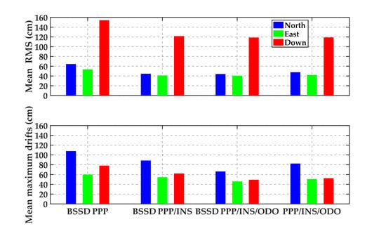
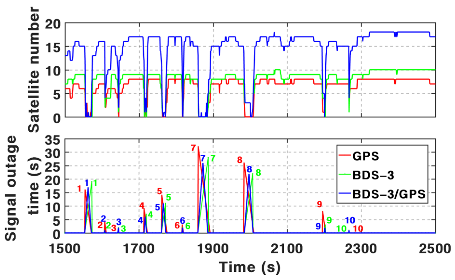
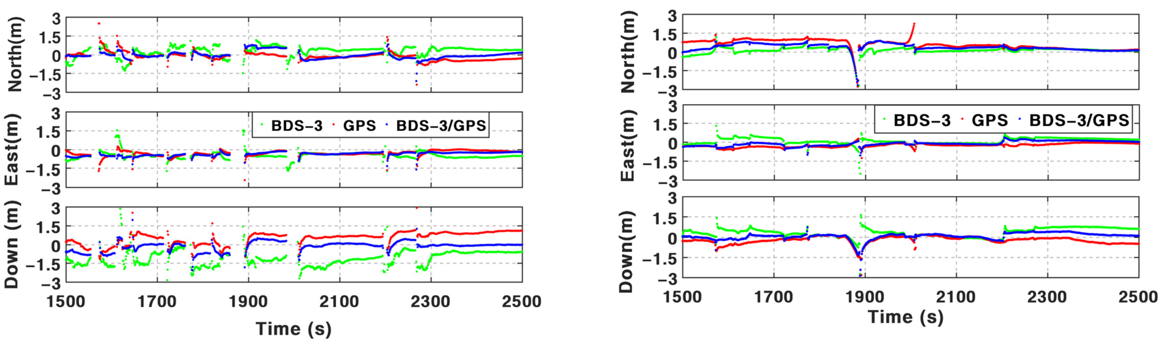
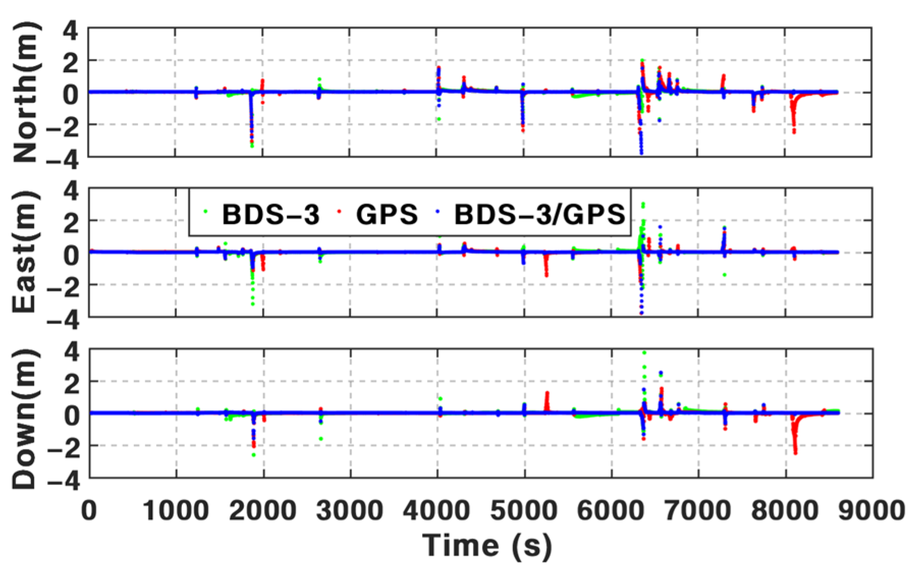
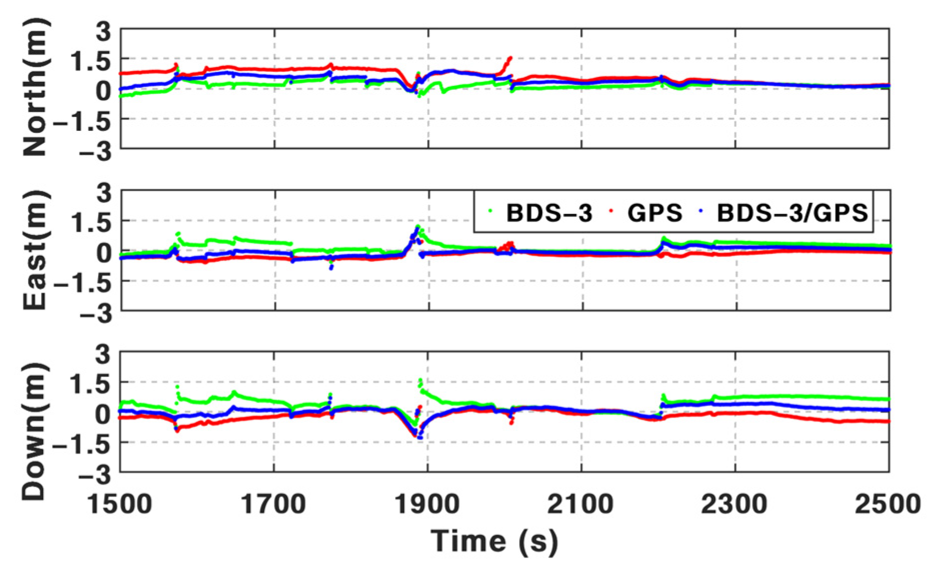
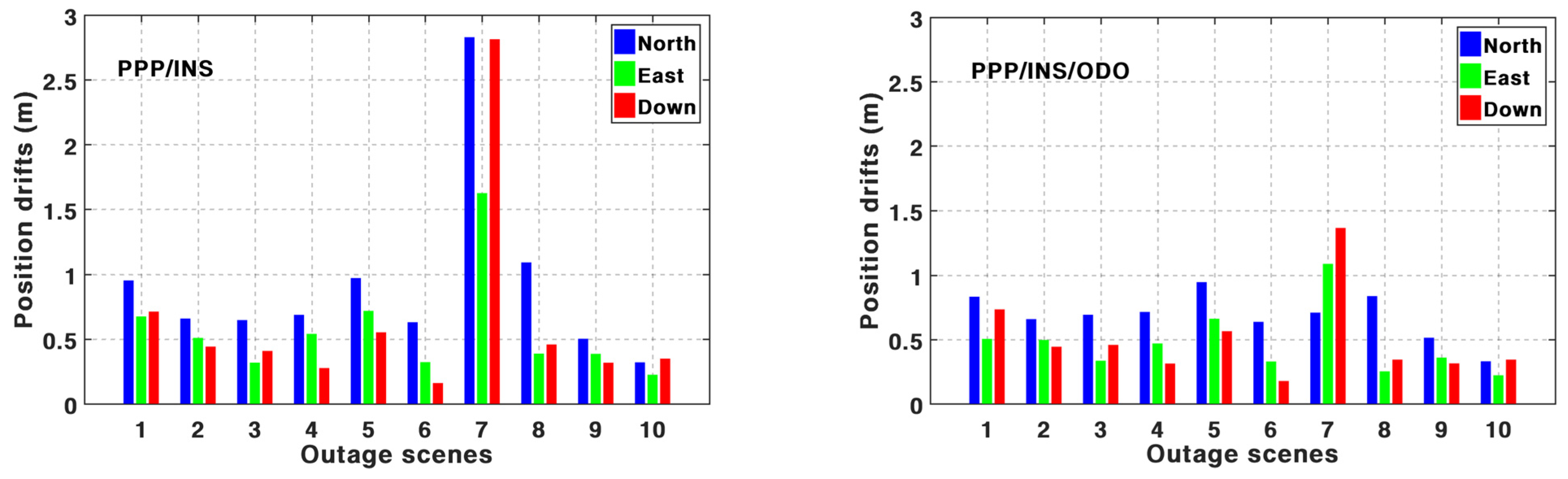
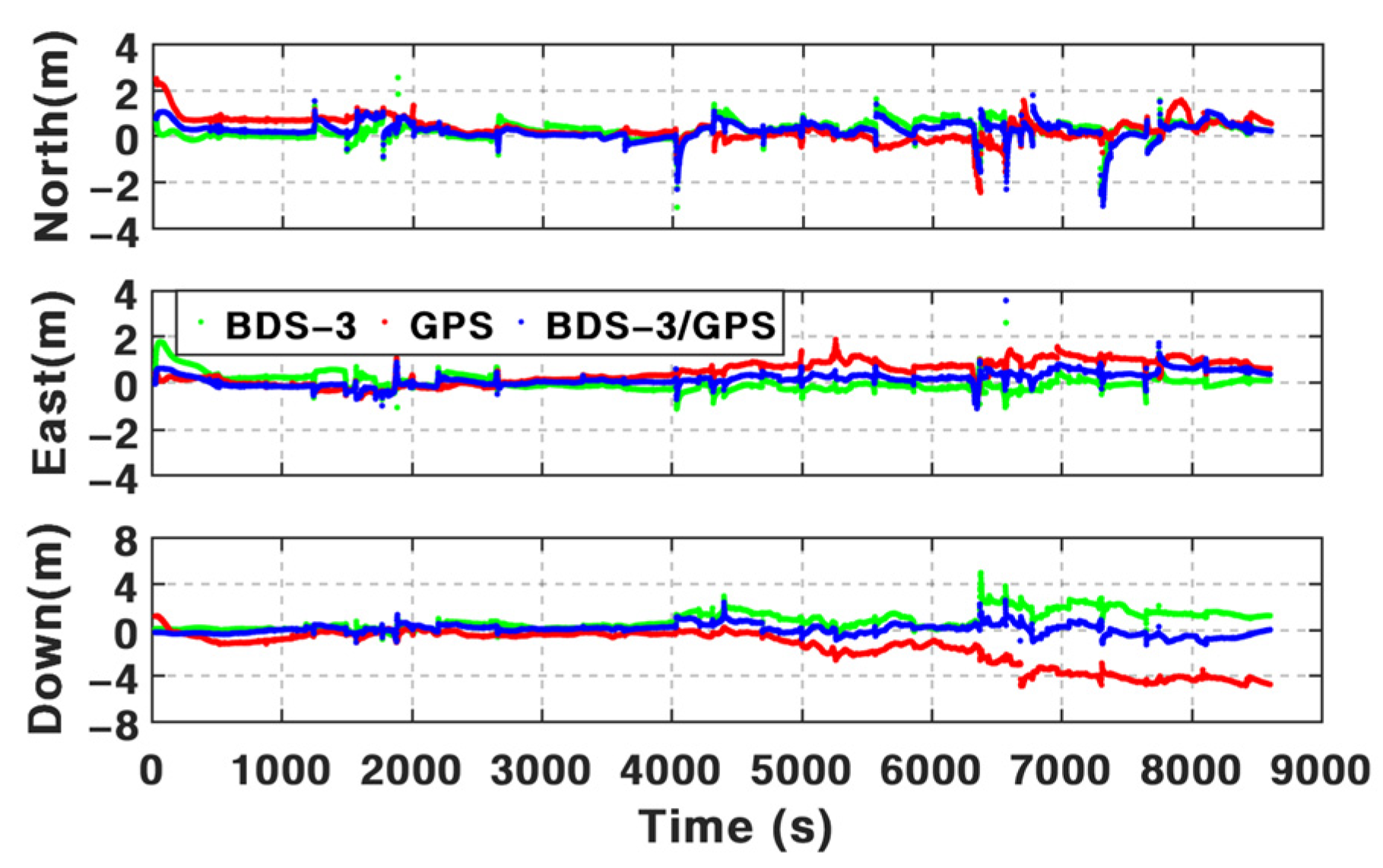
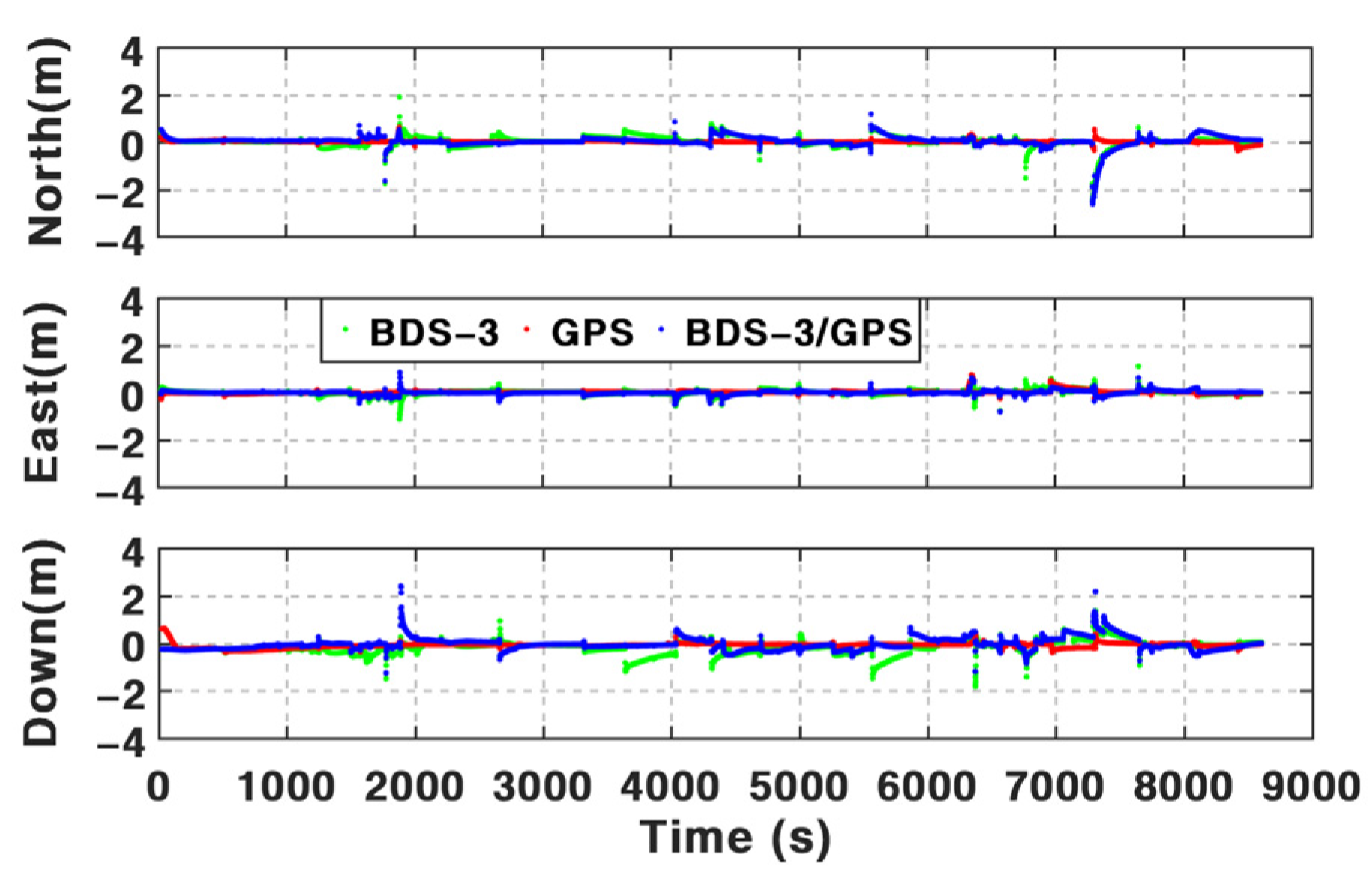
Based on the BDS-3 PPP-B2b service, real-time PPP can be used via B2b signals. However, it is still challenging in an urban environment. According to the assessments above and the results summarized in

Table 7. Statistic of position and attitude errors.

	Mean RMS (cm)			Mean Maximum Drifts (cm)
Positioning	North	East	Down	North	East	Down
BSSD PPP	64.33	53.47	154.11	107.96	59.90	78.22
BSSD PPP/INS TCI	44.54	41.29	121.66	88.52	54.54	62.00
BSSD PPP/INS/ODO TCI	44.01	40.79	118.83	66.29	45.84	49.17
Undifferenced PPP/INS/ODO TCI	47.69	42.09	119.15	82.38	50.66	52.30
	Mean RMS (°)			Mean Maximum Drifts (°)
Attitude	Roll	Pitch	Heading	Roll	Pitch	Heading
BSSD PPP/INS TCI	0.025	0.049	0.184	0.047	0.077	0.313
BSSD PPP/INS/ODO TCI	0.026	0.048	0.138	0.049	0.076	0.174
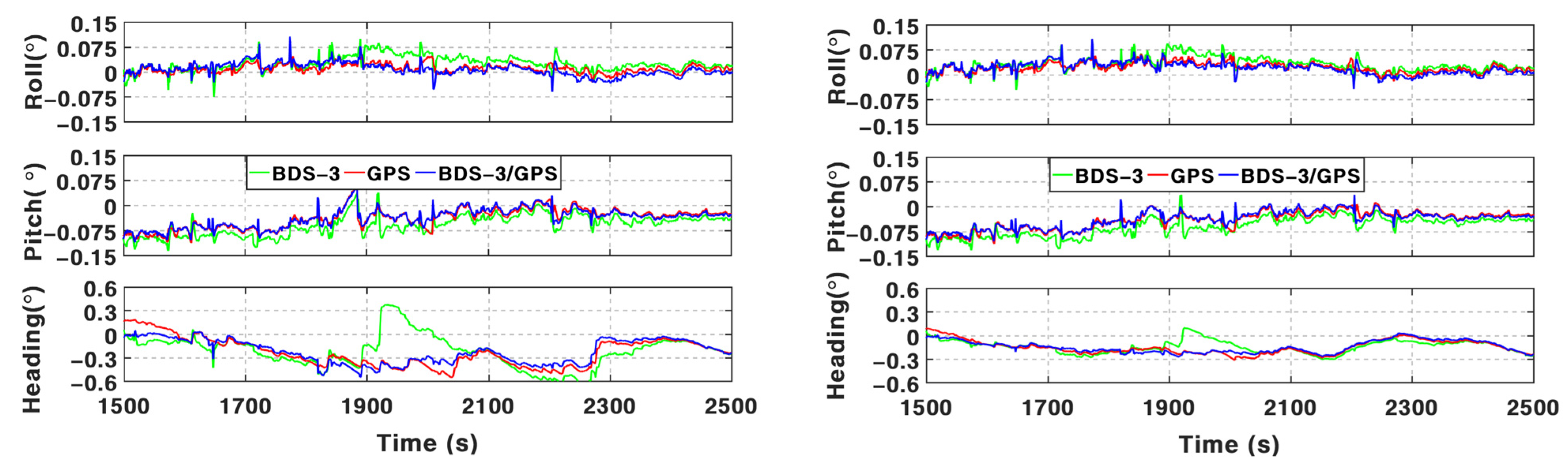
Undifferenced PPP/INS/ODO TCI	0.031	0.048	0.135	0.058	0.082	0.163

, the positioning performance of BSSD PPP can be enhanced visibly by the addition of INS and odometer, especially in periods with frequent GNSS outages. The mean position RMS of BSSD PPP is 64.33 cm, 53.47 cm, and 154.11 cm in three components based on PPP-B2b service. By integrating INS, the mean position RMS can be improved by 31.2%, 23.3%, and 27.3%. Such percentages can be furtherly increased by 1.34%, 1.41%, and 1.73% after using an odometer. The test data from 1500 s to 2500 s are adopted to validate the performance in the periods with frequent GNSS outages. The mean position maximum drifts during these periods decreased from 107.96 cm, 59.90 cm, and 78.22 cm of BSSD PPP to 88.52 cm, 54.54 cm, and 62.00 cm of BSSD PPP/INS TCI. After adding an odometer, such values are 66.29 cm, 45.84 cm, and 49.17 cm.

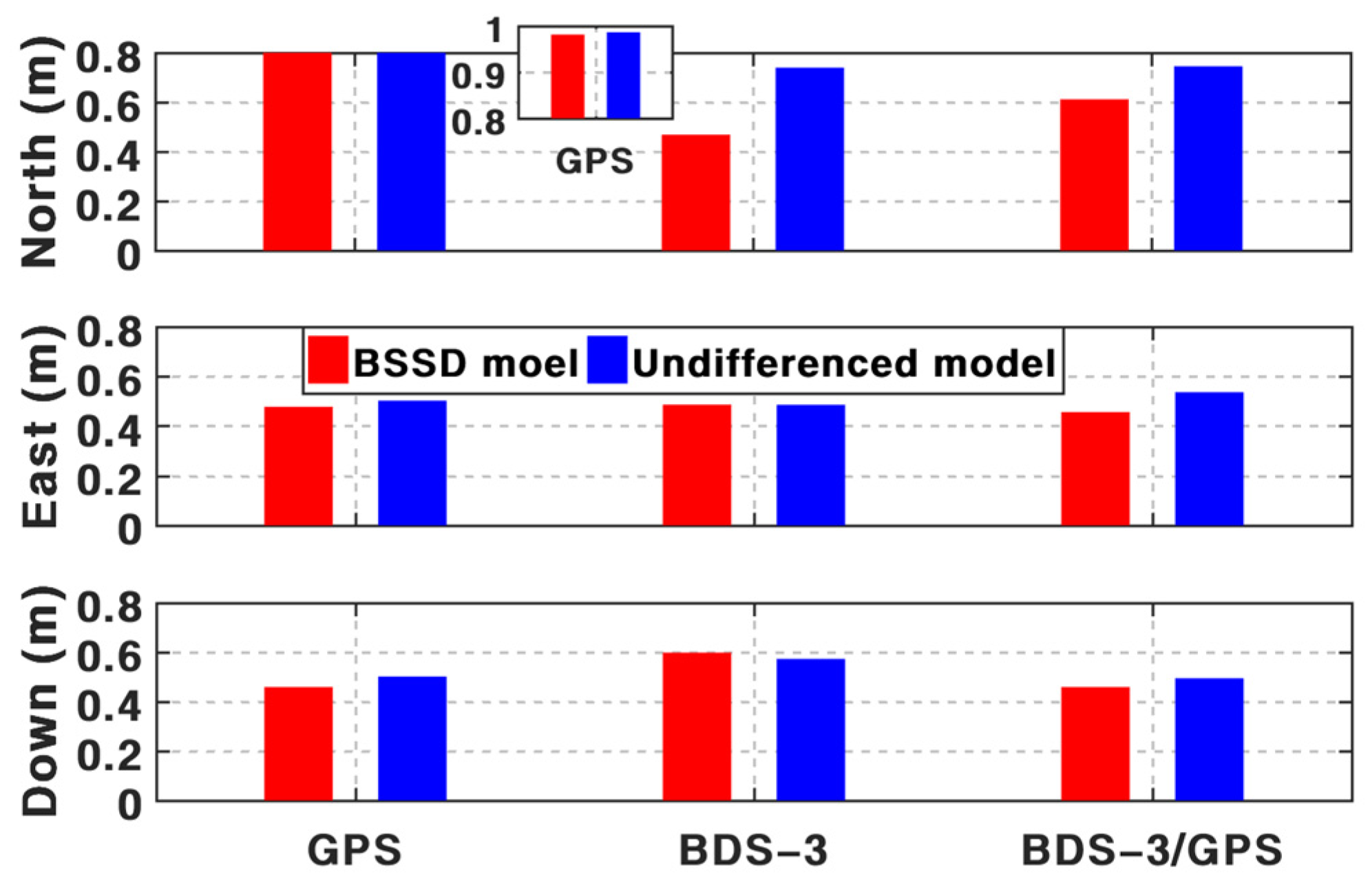
Anyway, the position accuracy of PPP/INS/ODO TCI based on the BSSD model is slightly higher than the solutions based on the undifferenced model. Compared with undifferenced PPP/INS/ODO TCI, the mean position RMS of BSSD PPP/INS/ODO TCI is improved by 7.71%, 3.09%, and 0.27%. The mean maximum drifts can be reduced from 82.38 cm, 50.66 cm, and 52.30 cm to 66.29 cm, 45.84 cm, and 49.17 cm by utilizing the BSSD model.

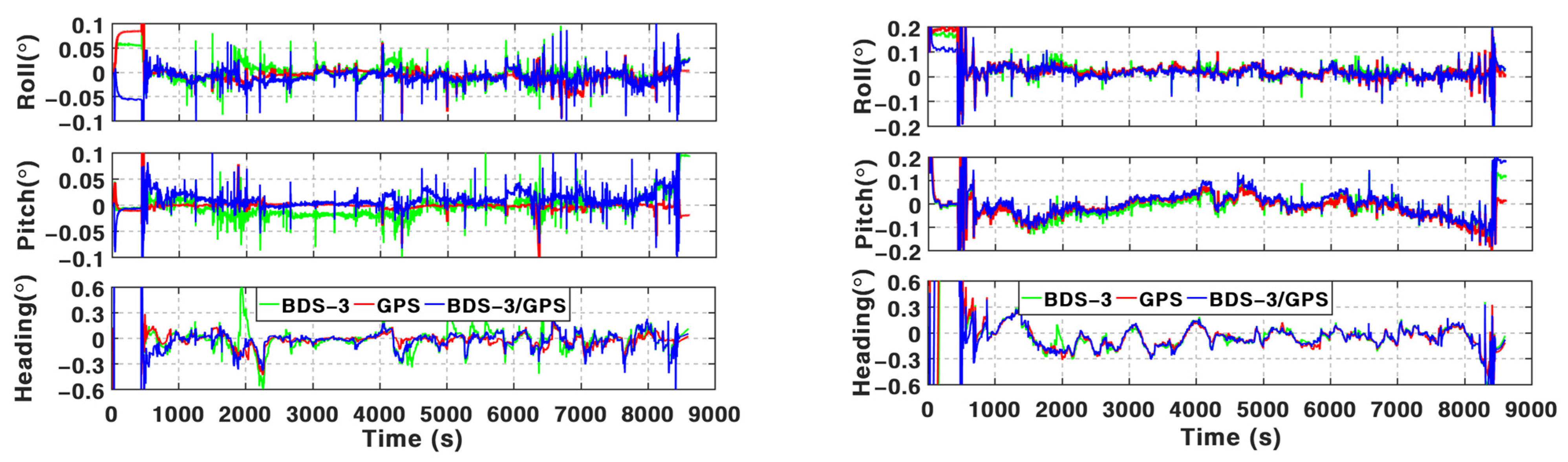
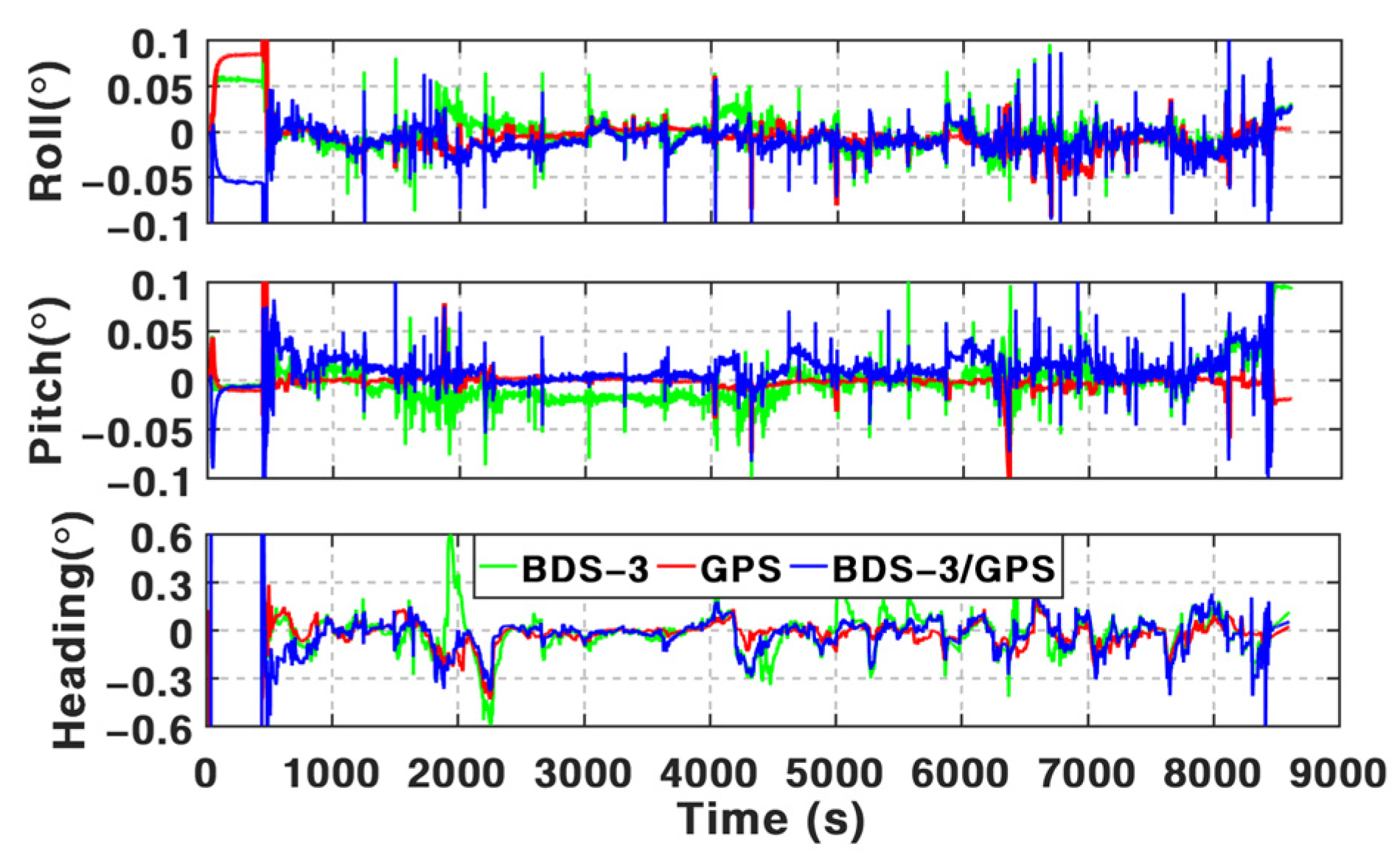
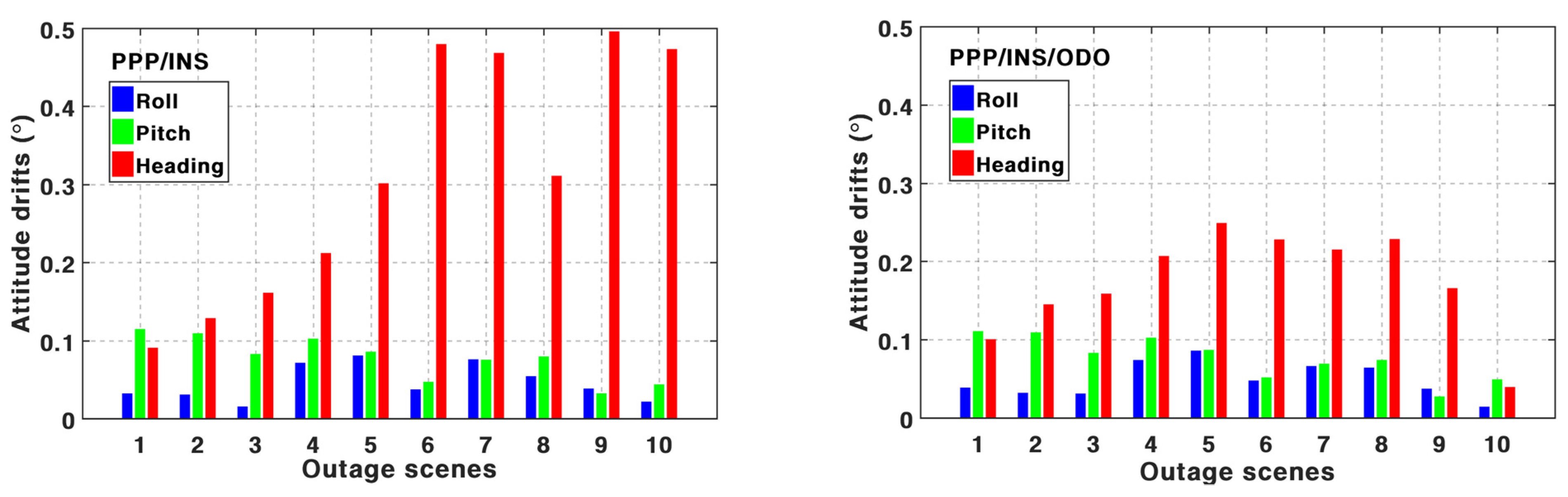
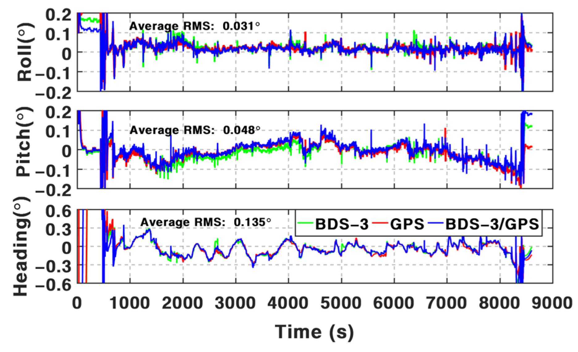
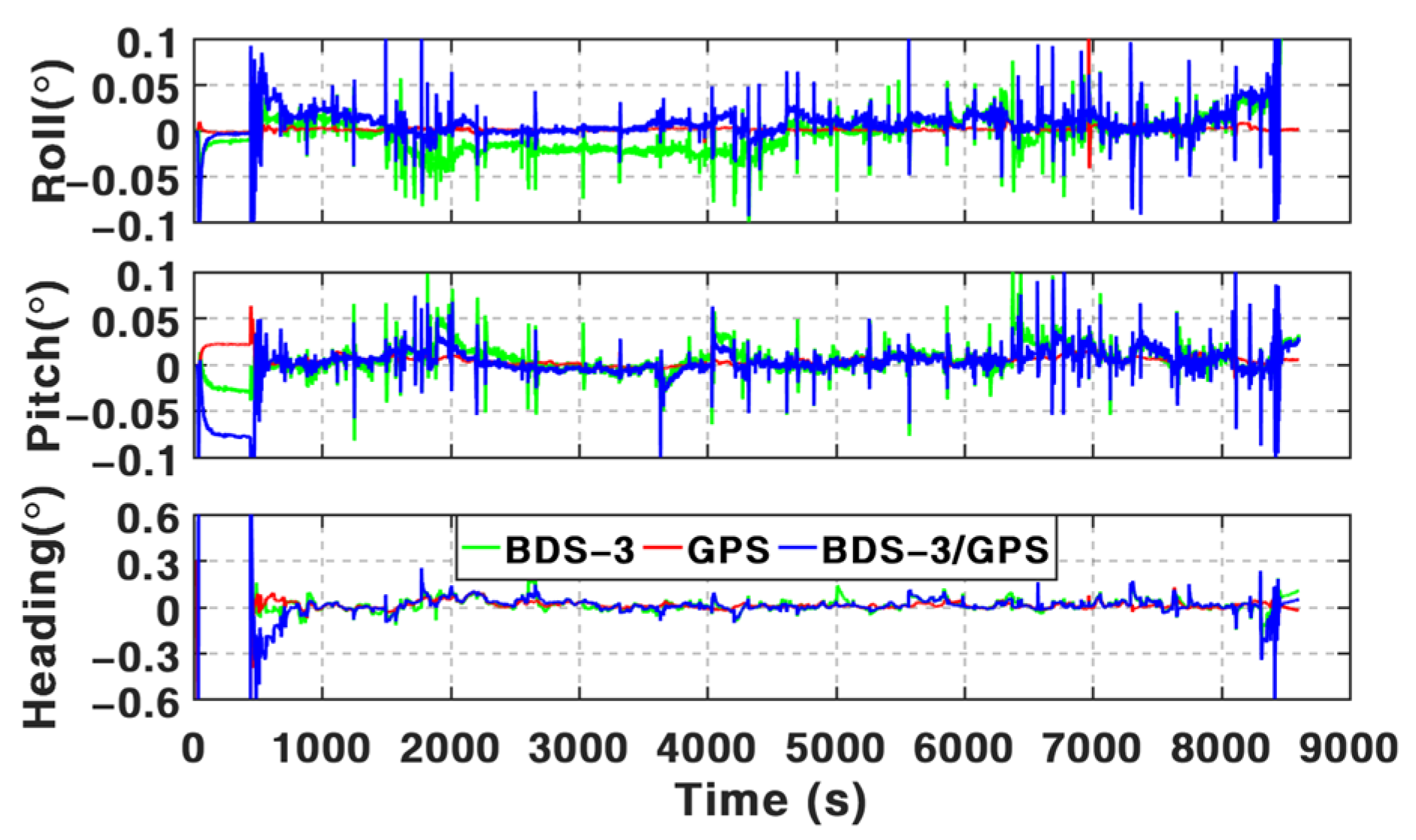
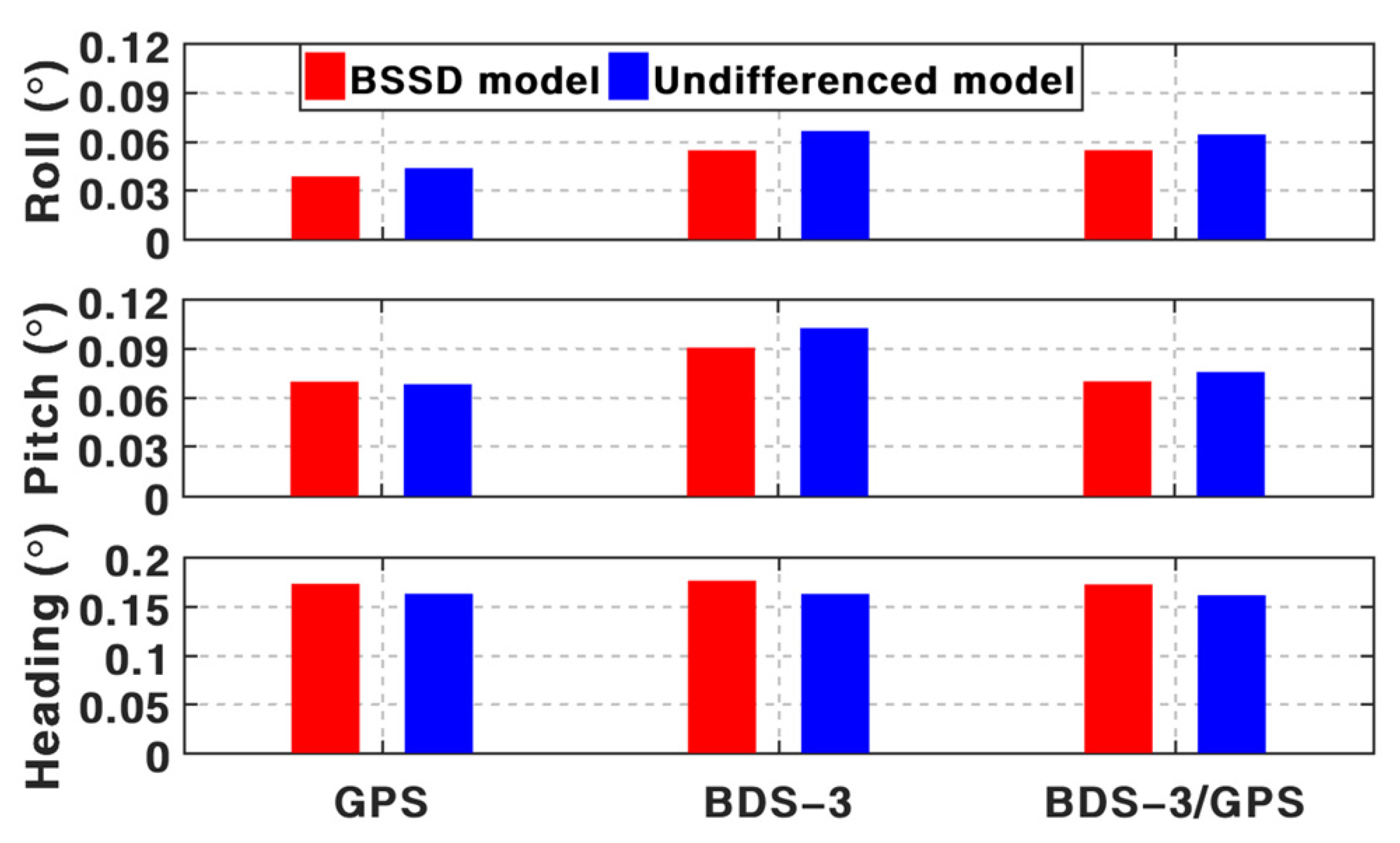
For attitude determination, the mean attitude RMS of PPP/INS TCI is 0.025°, 0.049°, and 0.184° in three components. The addition of an odometer brings a 25% improvement to the RMS of heading angles and reduces the mean maximum drifts from 0.313° to 0.174°. The results of the other two components are comparable. Moreover, the accuracy of PPP/INS/ODO TCI with and without the BSSD model is similar to each other.

5. Conclusions

In this contribution, we implied the tightly coupled integration of BDS-3/GPS, low-cost IMU, and odometer based on the inter-satellite differenced PPP model and the orbit/clock corrections of PPP-B2b. A vehicle experiment in urban circumstances was implemented to validate the performance of positioning and attitude determination of the developed model. The following conclusions can be obtained. (1) With the addition of INS, the improvements of BSSD PPP position accuracy on average are more than 31.2%, 23.3%, and 27.3% in the north, east, and down directions. Further enhancements in position accuracy are achievable with the aid of an odometer, especially while suffering GNSS outages. (2) By using the odometer, the accuracies of pitch and heading angles are improved by about 2.04% and 25%. (3) In comparison with the PPP/INS/ODO TCI based on the undifferenced PPP model, the developed BSSD model can provide results with higher accuracy, especially in the re-convergence periods. For attitude determination, comparable results can be obtained by both the BSSD model and the undifferenced model.

References

1. Yang, Y.; Xu, Y.; Li, J.; Yang, C. Progress and Performance Evaluation of BeiDou Global Navigation Satellite System: Data Analysis Based on BDS-3 Demonstration System. Sci. China Earth Sci. 2018, 61, 614–624. [Google Scholar] [CrossRef]
2. Yang, Y.; Li, J.; Wang, A.; Xu, J.; He, H.; Guo, H.; Shen, J.; Dai, X. Preliminary assessment of the navigation and positioning performance of BeiDou regional navigation satellite system. Sci. China Earth Sci. 2014, 57, 144–152. [Google Scholar] [CrossRef]
3. Yang, Y.; Tang, J.; Montenbruck, O. Chinese navigation satellite systems. In Handbook of Global Navigation Satellite Systems; Teunissen, M., Ed.; Springer: Cham, Switzerland, 2017; Chapter 10; pp. 273–304. [Google Scholar]
4. Lv, J.; Gao, Z.; Kan, J.; Lan, R.; Li, Y.; Lou, Y.; Yang, H.; Peng, J. Modeling and Assessment of Multi-Frequency GPS/BDS-2/BDS-3 Kinematic Precise Point Positioning Based on Vehicle-Borne Data. Measurement 2022, 189, 110453. [Google Scholar] [CrossRef]
5. Shi, C.; Wu, X.; Zheng, F.; Wang, X.; Wang, J. Modeling of BDS-2/BDS-3 Single-Frequency PPP with B1I and B1C Signals and Positioning Performance Analysis. Meas. J. Int. Meas. Confed. 2021, 178, 109355. [Google Scholar] [CrossRef]
6. Jiao, G.; Song, S.; Jiao, W. Improving BDS-2 and BDS-3 Joint Precise Point Positioning with Time Delay Bias Estimation. Meas. Sci. Technol. 2019, 31, 25001. [Google Scholar] [CrossRef]
7. Lu, M.; Li, W. Overview of BDS III New Signals. Navigation 2019, 66, 19–35. [Google Scholar] [CrossRef] [Green Version]
8. Zumberge, J.F.; Heflin, M.B.; Jefferson, D.C.; Watkins, M.M.; Webb, F.H. Precise Point Positioning for the Efficient and Robust Analysis of GPS Data from Large Networks. J. Geophys. Res. Solid Earth 1997, 102, 5005–5017. [Google Scholar] [CrossRef] [Green Version]
9. Gao, Y.; Shen, X. A New Method for Carrier-Phase-Based Precise Point Positioning. Navigation 2002, 49, 109–116. [Google Scholar] [CrossRef]
10. Li, X.; Ge, M.; Zhang, H.; Wickert, J. A Method for Improving Uncalibrated Phase Delay Estimation and Ambiguity-Fixing in Real-Time Precise Point Positioning. J. Geod. 2013, 87, 405–416. [Google Scholar] [CrossRef]
11. Elsobeiey, M.; El-Rabbany, A. Efficient Between-Satellite Single-Difference Precise Point Positioning Model. J. Surv. Eng. 2014, 140, 04014007. [Google Scholar] [CrossRef]
12. Kouba, J. A Guide to Using International GNSS Service (IGS) Products. IGS. 2015. Available online: http://igscb.jpl.nasa.gov/igscb/resource/pubs/UsingIGSProductsVer21.pdf (accessed on 9 September 2022).
13. Kouba, J.; Héroux, P. Precise Point Positioning Using IGS Orbit and Clock Products. GPS Solut. 2001, 5, 12–28. [Google Scholar] [CrossRef]
14. Zhang, W.; Lou, Y.; Song, W.; Sun, W.; Zou, X.; Gong, X. Initial Assessment of BDS-3 Precise Point Positioning Service on GEO B2b Signal. Adv. Sp. Res. 2022, 69, 690–700. [Google Scholar] [CrossRef]
15. Nie, Z.; Xu, X.; Wang, Z.; Du, J. Initial Assessment of BDS PPP-B2b Service: Precision of Orbit and Clock Corrections, and PPP Performance. Remote Sens. 2021, 13, 2050. [Google Scholar] [CrossRef]
16. Tao, J.; Liu, J.; Hu, Z.; Zhao, Q.; Chen, G.; Ju, B. Initial Assessment of the BDS-3 PPP-B2b RTS Compared with the CNES RTS. GPS Solut. 2021, 25, 131. [Google Scholar] [CrossRef]
17. Ren, Z.; Gong, H.; Peng, J.; Tang, C.; Huang, X.; Sun, G. Performance Assessment of Real-Time Precise Point Positioning Using BDS PPP-B2b Service Signal. Adv. Sp. Res. 2021, 68, 3242–3254. [Google Scholar] [CrossRef]
18. Wang, L.; Li, Z.; Ge, M.; Neitzel, F.; Wang, X.; Yuan, H. Investigation of the Performance of Real-Time BDS-Only Precise Point Positioning Using the IGS Real-Time Service. GPS Solut. 2019, 23, 66. [Google Scholar] [CrossRef]
19. Zhang, L.; Yang, H.; Gao, Y.; Yao, Y.; Xu, C. Evaluation and Analysis of Real-Time Precise Orbits and Clocks Products from Different IGS Analysis Centers. Adv. Sp. Res. 2018, 61, 2942–2954. [Google Scholar] [CrossRef]
20. Gao, Z.; Zhang, H.; Ge, M.; Niu, X.; Shen, W.; Wickert, J.; Schuh, H. Tightly Coupled Integration of Ionosphere-Constrained Precise Point Positioning and Inertial Navigation Systems. Sensors 2015, 15, 5783–5802. [Google Scholar] [CrossRef] [Green Version]
21. Gao, Z.; Ge, M.; Shen, W.; Zhang, H.; Niu, X. Ionospheric and Receiver DCB-Constrained Multi-GNSS Single-Frequency PPP Integrated with MEMS Inertial Measurements. J. Geod. 2017, 91, 1351–1366. [Google Scholar] [CrossRef]
22. Shin, E.-H. Estimation Techniques for Low-Cost Inertial Navigation. Ph.D. Thesis, The University of Calgary, Calgary, AB, Canada, May 2005. [Google Scholar]
23. Cox, D.B.J. Integration of GPS with Inertial Navigation Systems. Navigation 1978, 25, 236–245. [Google Scholar] [CrossRef]
24. Gu, S.; Dai, C.; Fang, W.; Zheng, F.; Wang, Y.; Zhang, Q.; Lou, Y.; Niu, X. Multi-GNSS PPP/INS Tightly Coupled Integration with Atmospheric Augmentation and Its Application in Urban Vehicle Navigation. J. Geod. 2021, 95, 64. [Google Scholar] [CrossRef]
25. Le, A.Q.; Lorga, J. Combining Inertial Navigation System With GPS Precise Point Positioning: Flight Test Results. In Proceedings of the ION GNSS 2006, Fort Worth, TX, USA, 26–29 September 2006; pp. 3035–3042. [Google Scholar]
26. Martell, H. Tightly Coupled Processing of Precise Point Position (PPP) and INS Data. In Proceedings of the ION GNSS 2009, Savannah, GA, USA, 22–25 September 2009; pp. 1898–1905. [Google Scholar]
27. Du, S. Integration of Precise Point Positioning and Low Cost MEMS IMU. Master’s Thesis, The University of Calgary, Calgary, AB, Canada, November 2010. [Google Scholar]
28. Abd Rabbou, M.; El-Rabbany, A. Tightly Coupled Integration of GPS Precise Point Positioning and MEMS-Based Inertial Systems. GPS Solut. 2015, 19, 601–609. [Google Scholar] [CrossRef]
29. BeiDou Navigation Satellite System Signal in Space Interface Control Document: Precise Point Positioning Service Signal PPP-B2b (Version 1.0). 2020. Available online: http://en.beidou.gov.cn/SYSTEMS/ICD/202008/P020200803538771492778.pdf (accessed on 20 October 2021).
30. Gao, Z.; Zhang, H.; Ge, M.; Niu, X.; Shen, W.; Wickert, J.; Schuh, H. Tightly Coupled Integration of Multi-GNSS PPP and MEMS Inertial Measurement Unit Data. GPS Solut. 2017, 21, 377–391. [Google Scholar] [CrossRef]
31. Sun, W.; Yang, Y. BDS PPP/INS Tight Coupling Method Based on Non-Holonomic Constraint and Zero Velocity Update. IEEE Access 2020, 8, 128866–128876. [Google Scholar] [CrossRef]
32. Gao, Z.; Ge, M.; Li, Y.; Chen, Q.; Zhang, Q.; Niu, X.; Zhang, H.; Shen, W.; Schuh, H. Odometer, Low-Cost Inertial Sensors, and Four-GNSS Data to Enhance PPP and Attitude Determination. GPS Solut. 2018, 22, 57. [Google Scholar] [CrossRef]
33. Witchayangkoon, B. Elements of GPS Precise Point Positioning. Ph.D. Thesis, Spatial Information Science and Engineering, University of Maine, Orono, ME, USA, 2000. [Google Scholar]
34. Pintor, P.; González, E.; Senado, A.; Bohlig, P.; Sperl, A.; Henkel, P.; Simón, J.; Hernández, C.; de Blas, J.; Vázquez, J. Galileo High Accuracy Service (HAS) Algorithm and Receiver Development and Testing. In Proceedings of the 35th International Technical Meeting of the Satellite Division of The Institute of Navigation (ION GNSS+ 2022), Denver, CO, USA, 19–23 September 2022; pp. 836–851. [Google Scholar]
35. Cai, C.; Gao, Y. Modeling and Assessment of Combined GPS/GLONASS Precise Point Positioning. GPS Solut. 2013, 17, 223–236. [Google Scholar] [CrossRef]
36. Chen, J.; Pei, X.; Zhang, Y.; Wu, B. GPS/GLONASS System Bias Estimation and Application in GPS/GLONASS Combined Positioning. Lect. Notes Electr. Eng. 2013, 244, 323–333. [Google Scholar]
37. Choy, S.; Zhang, S.; Lahaye, F.; Héroux, P. A Comparison between GPS-Only and Combined GPS+GLONASS Precise Point Positioning. J. Spat. Sci. 2013, 58, 169–190. [Google Scholar] [CrossRef]
38. Zhou, F.; Dong, D.; Li, P.; Li, X.; Schuh, H. Influence of Stochastic Modeling for Inter-System Biases on Multi-GNSS Undifferenced and Uncombined Precise Point Positioning. GPS Solut. 2019, 23, 59. [Google Scholar] [CrossRef]
39. Jiang, N.; Xu, Y.; Xu, T.; Xu, G.; Sun, Z.; Schuh, H. GPS/BDS Short-Term ISB Modelling and Prediction. GPS Solut. 2017, 21, 163–175. [Google Scholar] [CrossRef] [Green Version]
40. Niu, X.; Goodall, C.; Nassar, S.; El-Sheimy, N. An efficient methodfor evaluating the performance of MEMS IMUs. In Proceedings of the Position location and Navigation Symposium, 2006 IEEE/ION, San Diego, CA, USA, 25–27 April 2016; pp. 766–771. [Google Scholar]
41. Sukkarieh, S. Low Cost, High Integrity, Aided Inertial Navigation Systems for Autonomous Land Vehicles. Ph.D. Thesis, University of Sydney, Sydney, Australia, January 2000. [Google Scholar]
42. Mohamed, A.; Schwarz, K. Adaptive Kalman Filtering for INS/GPS. J. Geod. 1999, 73, 193–203. [Google Scholar] [CrossRef]
43. Lu, C.; Li, X.; Nilsson, T.; Ning, T.; Heinkelmann, R.; Ge, M.; Glaser, S.; Schuh, H. Real-Time Retrieval of Precipitable Water Vapor from GPS and BeiDou Observations. J. Geod. 2015, 89, 843–856. [Google Scholar] [CrossRef]
44. An, X.; Meng, X.; Jiang, W. Multi-Constellation GNSS Precise Point Positioning with Multi-Frequency Raw Observations and Dual-Frequency Observations of Ionospheric-Free Linear Combination. Satell. Navig. 2020, 1, 7. [Google Scholar] [CrossRef]
45. Li, X.; Ge, M.; Dai, X.; Ren, X.; Fritsche, M.; Wickert, J.; Schuh, H. Accuracy and Reliability of Multi-GNSS Real-Time Precise Positioning: GPS, GLONASS, BeiDou, and Galileo. J. Geod. 2015, 89, 607–635. [Google Scholar] [CrossRef]
46. Huang, L.; Lu, Z.; Li, B.; Xin, G.; An, W.; Lv, H.; Wang, N.; Zhou, X. The Performance Analysis of Multi-System Integrated Precise Point Positioning (PPP). Lect. Notes Electr. Eng. 2016, 390, 317–326. [Google Scholar]
Figure 1. Algorithm of BSSD PPP/INS/ODO TCI structure.
Remotesensing 15 00199 g001
Figure 2. The available satellites number of different GNSS along with the test trajectory.
Remotesensing 15 00199 g002
Figure 3. PDOP of different GNSS along with the test trajectory.
Remotesensing 15 00199 g003
Figure 4. RMS of GPS clock offset, and orbit errors of real-time products recovered by PPP-B2b service.
Remotesensing 15 00199 g004
Figure 5. RMS of BDS-3 clock offset and orbit errors of real-time products recovered by PPP-B2b service.
Remotesensing 15 00199 g005
Figure 6. Positioning errors of undifferenced PPP (left) and BSSD PPP (right) with different GNSS.
Remotesensing 15 00199 g006
Figure 7. Positioning errors of BSSD PPP/INS TCI with different GNSS.
Remotesensing 15 00199 g007
Figure 8. Positioning differences between BSSD PPP and BSSD PPP/INS TCI with different GNSS.
Remotesensing 15 00199 g008
Figure 9. Satellite numbers and outages time between the 1500 s and 2500 s.
Remotesensing 15 00199 g009
Figure 10. Positioning errors of BSSD PPP (left) and BSSD PPP/INS TCI (right) between the 1500 s and 2500 s.
Remotesensing 15 00199 g010
Figure 11. Positioning errors of BSSD PPP/INS/ODO TCI with different GNSS by using PPP-B2b corrections.
Remotesensing 15 00199 g011
Figure 12. Positioning differences between BSSD PPP/INS TCI and BSSD PPP/INS/ODO TCI with different GNSS.
Remotesensing 15 00199 g012
Figure 13. Positioning errors of BSSD PPP/INS/ODO TCI with frequent GNSS outages.
Remotesensing 15 00199 g013
Figure 14. Average maximum position drifts of different GNSS for BSSD PPP/INS TCI (left) and PPP/INS/ODO TCI (right) on different GNSS outage scenes.
Remotesensing 15 00199 g014
Figure 15. Positioning errors of undifferenced BSSD PPP/INS/ODO TCI with different GNSS using PPP-B2b correction.
Remotesensing 15 00199 g015
Figure 16. Positioning differences between undifferenced PPP/INS/ODO TCI and BSSD PPP/INS TCI/ODO.
Remotesensing 15 00199 g016
Figure 17. Mean maximum position drifts of different GNSS for BSSD PPP/INS/ODO TCI and undifferenced PPP/INS/ODO TCI.
Remotesensing 15 00199 g017
Figure 18. Attitude errors of BSSD PPP/INS TCI (left) and BSSD PPP/INS/ODO TCI (right) with different GNSS.
Remotesensing 15 00199 g018
Figure 19. Attitude differences between BSSD PPP/INS TCI and BSSD PPP/INS/ODO with different GNSS.
Remotesensing 15 00199 g019
Figure 20. Attitude errors of BSSD PPP/INS TCI (left) and BSSD PPP/INS/ODO TCI (right) with frequent GNSS outages in the periods between the 1500 s and 2500 s.
Remotesensing 15 00199 g020
Figure 21. Average of Maximum attitude drifts of different GNSS for BSSD PPP/INS TCI (left) and PPP/INS/ODO TCI (right) on different GNSS outage scenes.
Remotesensing 15 00199 g021
Figure 22. Attitude errors of undifferenced PPP/INS/ODO TCI with different GNSS.
Remotesensing 15 00199 g022
Figure 23. Attitudes differences between undifferenced PPP/INS/ODO TCI and BSSD PPP/INS/ODO TCI.
Remotesensing 15 00199 g023
Figure 24. Mean maximum attitude drifts of different GNSS for BSSD PPP/INS/ODO TCI and undifferenced PPP/INS/ODO TCI.
Remotesensing 15 00199 g024