
An Empirical Grid Model for Precipitable Water Vapor


Abstract
1. Introduction
2. Materials and Methods
2.1. ERA5 Reanalysis Products
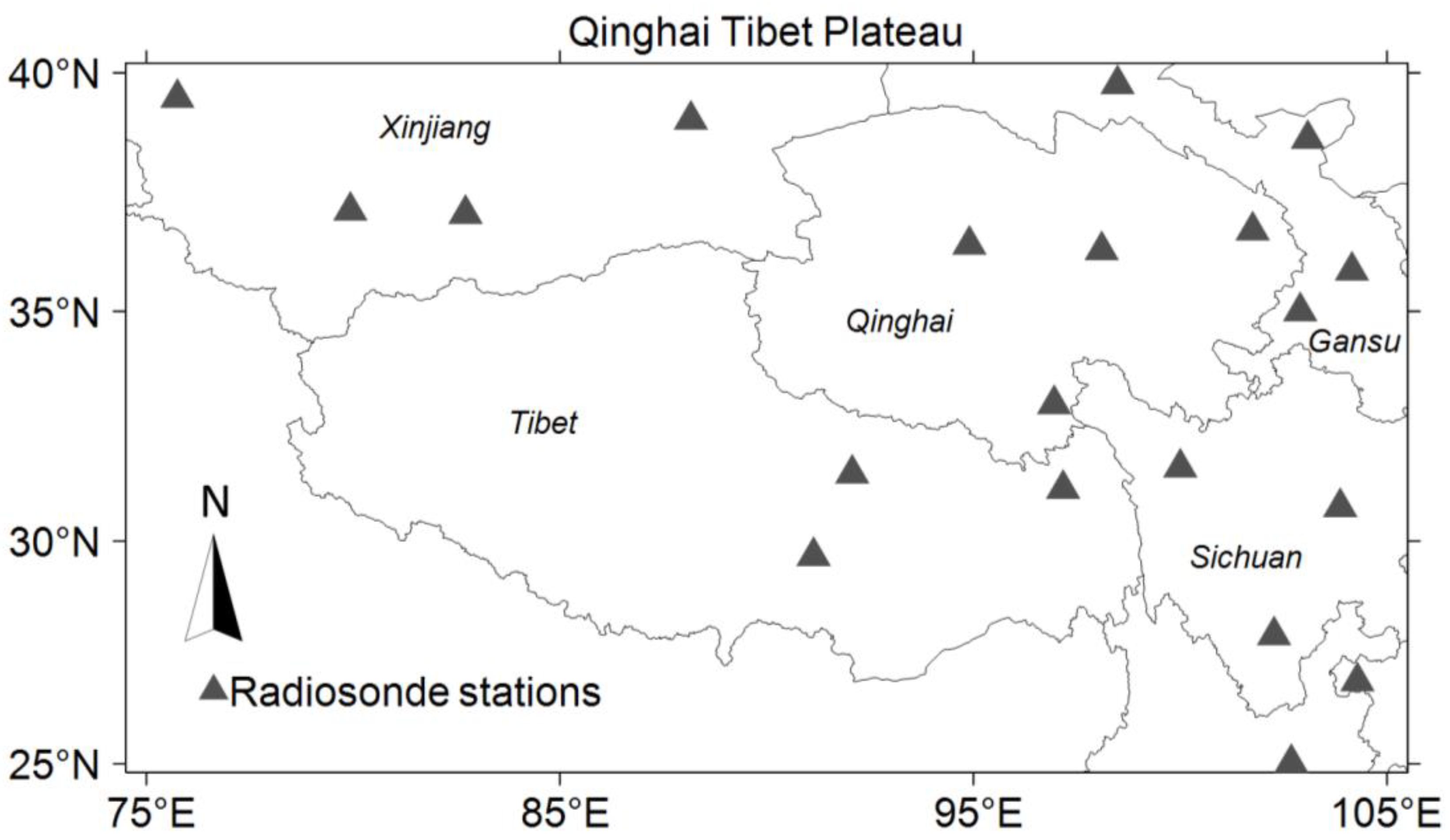
2.2. Radiosonde Profiles
2.3. ASV-PWV Deriving and Correction
- (1)
- Fundamentals of ASV-PWV model
- (2)
- PWV correction using spherical harmonic function
- (3)
- Vertical correction
3. Model Validation of ASV-PWV
3.1. Statistical Indicators
3.2. Validation with Radiosonde Profiles
3.3. Validation with the ERA5 Reanalysis PWV Products
4. Conclusions
Author Contributions
Funding
Acknowledgments
Conflicts of Interest
References
- Yao, Y.; Zhang, S.; Kong, J. Research Progress and Prospect of GNSS Space Environment Science. Acta Geod. Cartogr. Sin. 2017, 46, 1408–1420. [Google Scholar] [CrossRef]
- Dessler, A.E.; Sherwood, S.C. A matter of humidity. Science 2009, 323, 1020–1021. [Google Scholar] [CrossRef] [PubMed]
- Chung, E.; Soden, B.; Sohn, B.J.; Shi, L. Upper-tropospheric moistening in response to anthropogenic warming. Proc. Natl. Acad. Sci. USA 2014, 111, 11636–11641. [Google Scholar] [CrossRef] [PubMed]
- Trenberth, K.E.; Fasullo, J.; Smith, L. Trends and variability in column-integrated atmospheric water vapor. Clim. Dyn. 2005, 24, 741–758. [Google Scholar] [CrossRef]
- Allan, R.P.; Soden, B.J. Atmospheric Warming and the Amplification of Precipitation Extremes. Science 2008, 321, 1481–1484. [Google Scholar] [CrossRef]
- King, M.D.; Kaufman, Y.J.; Menzel, W.P.; Tanre, D. Remote sensing of cloud, aerosol, and water vapor properties from the moderate resolution imaging spectrometer (MODIS). IEEE Trans. Geosci. Remote Sens. 1992, 30, 2–27. [Google Scholar] [CrossRef]
- Berezin, I.A.; Timofeyev, Y.M.; Virolainen, Y.A.; Frantsuzova, I.S.; Volkova, K.A.; Poberovsky, A.V.; Holben, B.N.; Smirnov, A.; Slutsker, I. Error analysis of integrated water vapor measured by CIMEL photometer. Izvestiya Atmos. Ocean. Phys. 2017, 53, 58–64. [Google Scholar] [CrossRef]
- Campmany, E.; Bech, J.; Rodríguez-Marcos, J.; Sola, Y.; Lorente, J. A comparison of total precipitable water measurements from radiosonde and sunphotometers. Atmos. Res. 2010, 97, 385–392. [Google Scholar] [CrossRef]
- Ross, R.J.; Elliott, W.P. Radiosonde-Based Northern Hemisphere Tropospheric Water Vapor Trends. J. Clim. 2001, 14, 1602–1612. [Google Scholar] [CrossRef]
- Gurbuz, G. On Variations of the Decadal Precipitable Water Vapor (PWV) over Turkey. Adv. Space Res. 2021, 68, 292–300. [Google Scholar] [CrossRef]
- Easterling, D.; Peterson, T. A new method for detecting undocumented discontinuities in climatological time series. Int. J. Climatol. 1995, 15, 369–377. [Google Scholar] [CrossRef]
- Rowe, P.M.; Miloshevich, L.M.; Turner, D.D.; Walden, V.P. Dry Bias in Vaisala RS90 Radiosonde Humidity Profiles over Antarctica. J. Atmos. Ocean. Technol. 2008, 25, 1529–1541. [Google Scholar] [CrossRef][Green Version]
- Zhao, T.; Dai, A.; Wang, J. Trends in Tropospheric Humidity from 1970 to 2008 over China from a Homogenized Radiosonde Dataset. J. Clim. 2012, 25, 4549–4567. [Google Scholar] [CrossRef]
- Gao, B.; Kaufman, Y.J. Water vapor retrievals using Moderate Resolution Imaging Spectroradiometer (MODIS) near-infrared channels. J. Geophys. Res. Atmos. 2003, 108, 108:1–108:10. [Google Scholar] [CrossRef]
- Liu, B.; Wang, Y.; Lou, Z.; Zhan, W. The MODIS PWV correction based on CMONOC in Chinese mainland. Acta Geod. Cartogr. Sin. 2019, 48, 1207–1215. [Google Scholar] [CrossRef]
- Kumar, S.; Singh, A.K.; Prasad, A.K.; Singh, R.P. Variability of GPS derived water vapor and comparison with MODIS data over the Indo-Gangetic plains. Phys. Chem. Earth 2010, 55–57, 11–18. [Google Scholar] [CrossRef]
- Shi, F.; Xin, J.; Yang, L.; Cong, Z.; Liu, R.; Ma, Y.; Wang, Y.; Lu, X.; Zhao, L. The first validation of the precipitable water vapor of multisensor satellites over the typical regions in China. Remote Sens. Environ. 2017, 206, 107–122. [Google Scholar] [CrossRef]
- Khaniani, A.S.; Nikraftar, Z.; Zakeri, S. Evaluation of MODIS Near-IR water vapor product over Iran using ground-based GPS measurements. Atmos. Res. 2020, 231, 104657. [Google Scholar] [CrossRef]
- Dee, D.P.; Uppala, S.M.; Simmons, A.J.; Berrisford, P.; Poli, P.; Kobayashi, S.; Andrae, U.; Balmaseda, M.A. The ERA-Interim reanalysis: Configuration and performance of the data assimilation system. Q. J. R. Meteorol. Soc. 2011, 137, 553–597. [Google Scholar] [CrossRef]
- Zhang, L.; Wu, L.; Gan, B. Modes and Mechanisms of Global Water Vapor Variability over the Twentieth Century. J. Clim. 2013, 26, 5578–5593. [Google Scholar] [CrossRef]
- Sherwood, S.C.; Roca, R.; Weckwerth, T.M.; Andronova, N.G. Tropospheric water vapor, convection, and climate. Rev. Geophys. 2010, 48, RG2001. [Google Scholar] [CrossRef]
- Chen, B.; Liu, Z. Global water vapor variability and trend from the latest 36 year (1979 to 2014) data of ECMWF and NCEP reanalyses, radiosonde, GPS, and microwave satellite. J. Geophys. Res. Atmos. 2016, 121, 11442–11462. [Google Scholar] [CrossRef]
- Cortés, F.; Cortés, K.; Reeves, R.; Bustos, R.; Radford, S. Twenty years of precipitable water vapor measurements in the Chajnantor area. Astron. Astrophys. 2020, 640, A126. [Google Scholar] [CrossRef]
- Shikhovtsev, A.Y.; Khaikin, V.B.; Mironov, A.P.; Kovadlo, P.G. Statistical Analysis of the Water Vapor Content in North Caucasus and Crimea. Atmos. Ocean. Opt. 2022, 35, 168–175. [Google Scholar] [CrossRef]
- Ma, X.; Yao, Y.; Zhang, B.; He, C. Retrieval of high spatial resolution precipitable water vapor maps using heterogeneous earth observation data. Remote Sens. Environ. 2022, 278, 113100. [Google Scholar] [CrossRef]
- Yao, Y.; Xu, X.; Hu, Y. Establishment of a regional precipitable water vapor model based on the combination of GNSS and ECMWF data. Atmos. Meas. Tech. Discuss. 2018, 1–21. [Google Scholar] [CrossRef]
- Zhang, B.; Yao, Y.; Xin, L.; Xu, X. Precipitable water vapor fusion: An approach based on spherical cap harmonic analysis and Helmert variance component estimation. J. Geod. 2019, 93, 2605–2620. [Google Scholar] [CrossRef]
- Zhang, B.; Yao, Y. Precipitable water vapor fusion based on a generalized regression neural network. J. Geod. 2021, 95, 36. [Google Scholar] [CrossRef]
- Huang, L.; Wang, X.; Xiong, S.; Li, J.; Liu, L.; Mo, Z.; Fu, B.; He, H. High-precision GNSS PWV retrieval using dense GNSS sites and in-situ meteorological observations for the evaluation of MERRA-2 and ERA5 reanalysis products over China. Atmos. Res. 2022, 276, 106247. [Google Scholar] [CrossRef]
- Huang, L.; Zhu, G.; Liu, L.; Chen, H.; Jiang, W. A global grid model for the correction of the vertical zenith total delay based on a sliding window algorithm. GPS Solut. 2021, 25, 98. [Google Scholar] [CrossRef]
- Huang, L.; Mo, Z.; Xie, S.; Liu, L.; Chen, J.; Kang, C.; Wang, S. Spatiotemporal characteristics of GNSS-derived precipitable water vapor during heavy rainfall events in Guilin, China. Satell. Navig. 2021, 2, 13. [Google Scholar] [CrossRef]
- Huang, L.; Liu, L.; Chen, H.; Jiang, W. An improved atmospheric weighted mean temperature model and its impact on GNSS precipitable water vapor estimates for China. GPS Solut. 2019, 23, 51. [Google Scholar] [CrossRef]
- Leckner, B. The spectral distribution of solar radiation at the earth’s surface–elements of a model. Sol. Energy 1978, 20, 143–150. [Google Scholar] [CrossRef]
- Kouba, J. Implementation and testing of the gridded Vienna Mapping Function 1 (VMF1). J. Geod. Vol. 2018, 82, 193–205. [Google Scholar] [CrossRef]
- Dousa, J.; Elias, M. An improved model for calculating tropospheric wet delay. Geophys. Res. Lett. 2014, 41, 4389–4397. [Google Scholar] [CrossRef]
- Huang, L.; Mo, Z.; Liu, L.; Xie, S. An empirical model for the vertical correction of precipitable water vapor considering the time-varying lapse rate for Mainland China. Acta Geod. Cartogr. Sin. 2021, 50, 1320–1330. [Google Scholar] [CrossRef]
- Askne, J.; Nordius, H. Estimation of tropospheric delay for microwaves from surface weather data. Radio Sci. 1987, 22, 379–386. [Google Scholar] [CrossRef]
- Hersbach, H.; Dee, D. ERA5 Reanalysis is in Production. ECMWF Newsletter. 2016. Available online: https://www.ecmwf.int/en/newsletter/147/news/era145-reanalysis-production (accessed on 17 September 2022).
- Hersbach, H.; Bell, B.; Berrisford, P.; Hirahara, S.; Horányi, A.; Muñoz-Sabater, J.; Nicolas, J.; Peubey, C.; Radu, R.; Schepers, R.; et al. The ERA5 global reanalysis. Q. J. R. Meteorol. Soc. 2020, 146, 1999–2049. [Google Scholar] [CrossRef]
- Bill, B.; Hans, H.; Adrian, S.; Paul, B.; Per, D.; András, H.; Joaquín, M.; Julien, N.; Raluca, R.; Dinand, S.; et al. The ERA5 global reanalysis: Preliminary extension to 1950. Q. J. R. Meteorol. Soc. 2021, 147, 4186–4227. [Google Scholar] [CrossRef]
- Zhao, Q.; Yang, P.; Yao, W.; Yao, Y. Hourly PWV Dataset Derived from GNSS Observations in China. Sensors 2019, 20, 231. [Google Scholar] [CrossRef]
- Peng, Y.; Addisu, H.; Fadwa, A.; Joseph, A.; Anna, K.; Norman, T.F.; Hansjörg, K. Feasibility of ERA5 integrated water vapor trends for climate change analysis in continental Europe: An evaluation with GPS (1994–2019) by considering statistical significance. Remote Sens. Environ. 2021, 260, 112416. [Google Scholar] [CrossRef]
- Zhang, W.; Wang, L.; Yu, Y.; Xu, G.; Hu, X.; Fu, Z.; Cui, C. Global evaluation of the precipitable-water-vapor product from MERSI-II (Medium Resolution Spectral Imager) on board the Fengyun-3D satellite. Atmos. Meas. Tech. 2021, 14, 7821–7834. [Google Scholar] [CrossRef]
- Durre, I.; Yin, X.; Vose, R.S.; Applequist, S.; Arnfield, J. Enhancing the Data Coverage in the Integrated Global Radiosonde Archive. J. Atmos. Ocean. Technol. 2018, 35, 1753–1770. [Google Scholar] [CrossRef]
- Durre, I.; Vose, R.S.; Wuertz, D.B. Overview of the Integrated Global Radiosonde Archive. J. Clim. 2006, 19, 53–68. [Google Scholar] [CrossRef]
- Gui, K.; Che, H.; Chen, Q.; Zeng, Z.; Zheng, Y.; Long, Q.; Sun, T.; Liu, X.; Wang, Y.; Liao, T.; et al. Water vapor variation and the effect of aerosols in China. Atmos. Environ. 2017, 165, 322–335. [Google Scholar] [CrossRef]
- He, Q. Water Vapor Retrieved from Ground-based GNSS and Its Applications in Extreme Weather Studies. Ph.D. Dissertation, China University of Mining and Technology, Beijing, China. Available online: https://kns.cnki.net/KCMS/detail/detail.aspx?dbname=CDFDLAST2022&filename=1021773689.nh (accessed on 24 September 2022).
- Böhm, J.; Möller, G.; Schindelegger, M.; Pain, G.; Weber, R. Development of an improved blind model for slant delays in the troposphere (GPT2w). GPS Solut. 2015, 19, 433–441. [Google Scholar] [CrossRef]
- Liu, J.; Chen, R.; Wang, Z.; Zhang, H. Spherical cap harmonic model for mapping and predicting regional TEC. GPS Solut. 2011, 15, 109–119. [Google Scholar] [CrossRef]
- Zhao, Q.; Du, Z.; Wu, M.; Yao, Y.; Yao, W. Analysis of Influencing Factors and Accuracy Evaluation of PWV in Loess Plateau. Geomatics and Information Science of Wuhan University. 2021. Available online: http://kns.cnki.net/kcms/detail/42.1676.TN.20211028.20211233.20211008.html (accessed on 30 September 2022).
- Wang, S.; Xu, T.; Nie, W.; Jiang, C.; Zhang, Z. Evaluation of Precipitable Water Vapor from Five Reanalysis Products with Ground-Based GNSS Observations. Remote Sens. 2020, 12, 1817. [Google Scholar] [CrossRef]


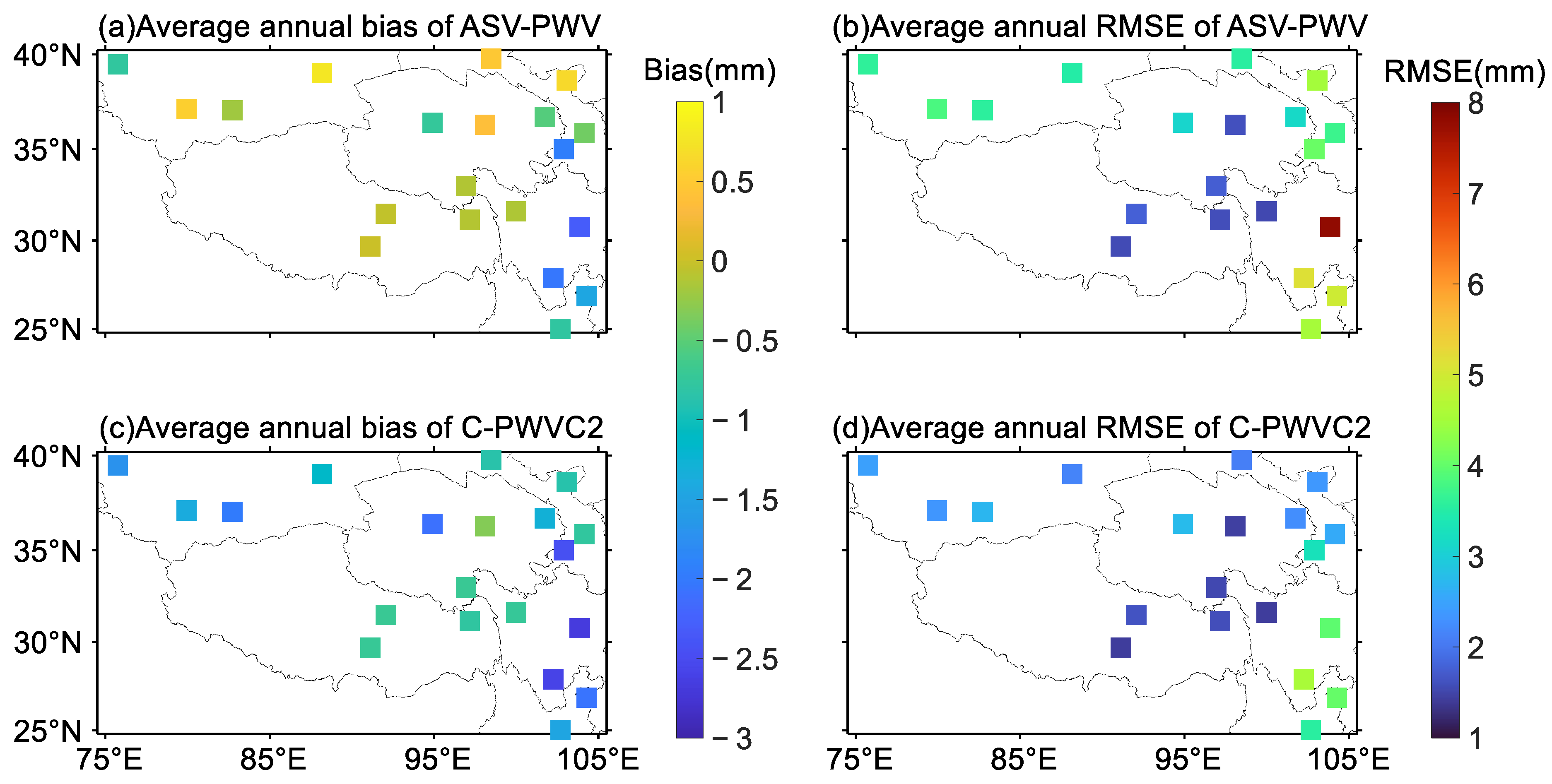
| Model | Bias (mm) | RMSE (mm) | ||||
|---|---|---|---|---|---|---|
| Avg | Max | Min | Avg | Max | Min | |
| ASV-PWV | −0.44 | 0.79 | −2.30 | 3.44 | 7.79 | 1.54 |
| C-PWVC2 | −1.36 | −0.32 | −2.68 | 2.51 | 4.58 | 1.42 |
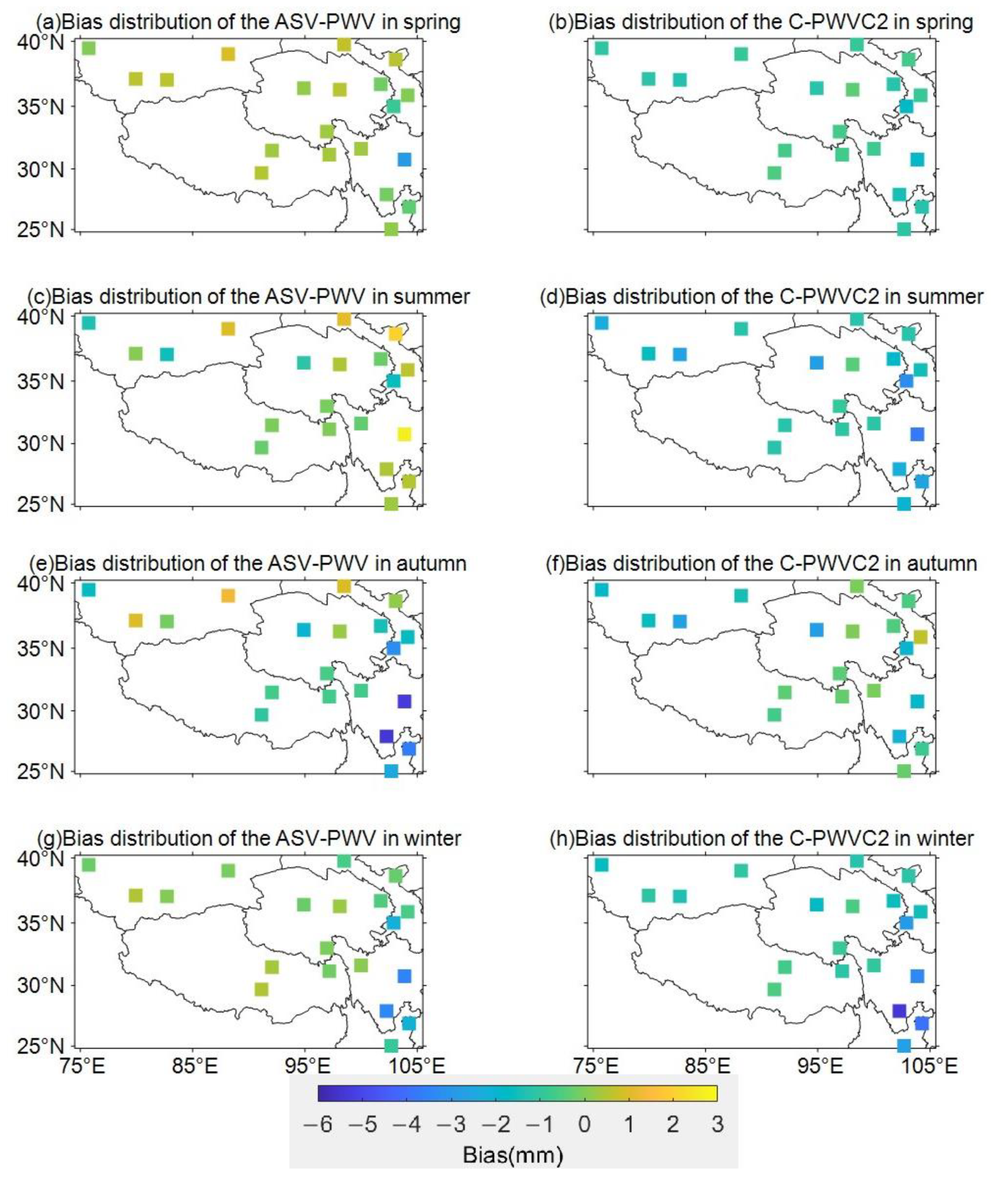
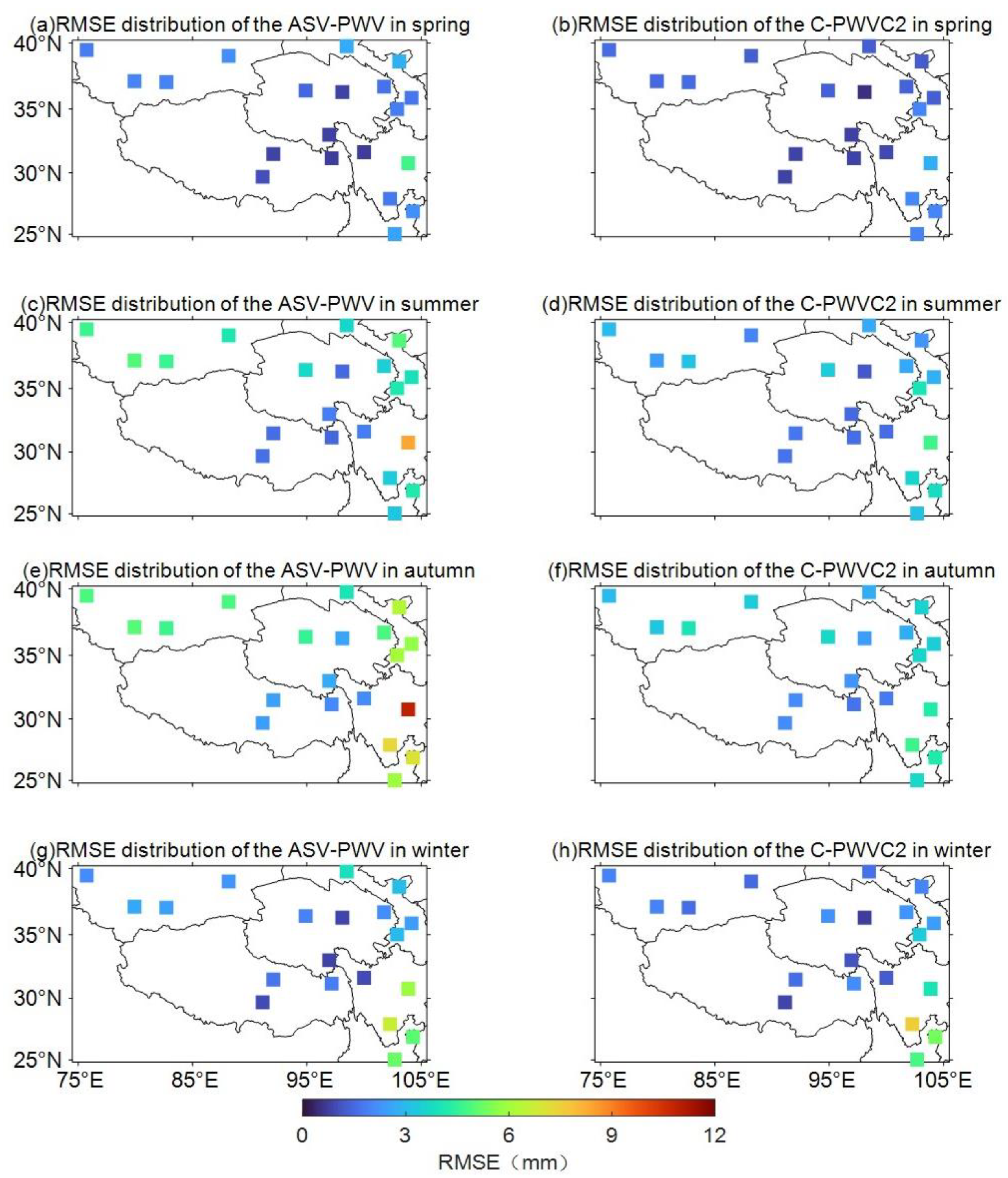
| Model | Indicator (mm) | Spring | Summer | Autumn | Winner | ||||||||
|---|---|---|---|---|---|---|---|---|---|---|---|---|---|
| Avg | Max | Min | Avg | Max | Min | Avg | Max | Min | Avg | Max | Min | ||
| ASV-PWV | Bias | 0.10 | 0.95 | −2.86 | 0.14 | 2.71 | −1.61 | −1.34 | 1.34 | −5.37 | −0.65 | 0.50 | −3.49 |
| RMSE | 1.81 | 4.73 | 0.72 | 3.55 | 8.35 | 1.43 | 4.83 | 10.89 | 2.10 | 2.81 | 6.68 | 0.83 | |
| C-PWVC2 | Bias | −1.01 | −0.34 | −1.88 | −1.81 | −0.42 | −3.72 | −0.99 | 0.67 | −2.81 | −1.76 | −0.53 | −5.40 |
| RMSE | 1.39 | 2.77 | 0.48 | 2.64 | 4.69 | 1.20 | 3.13 | 4.66 | 1.68 | 2.51 | 7.58 | 0.70 | |
Publisher’s Note: MDPI stays neutral with regard to jurisdictional claims in published maps and institutional affiliations. |
© 2022 by the authors. Licensee MDPI, Basel, Switzerland. This article is an open access article distributed under the terms and conditions of the Creative Commons Attribution (CC BY) license (https://creativecommons.org/licenses/by/4.0/).
Share and Cite
Wang, X.; Chen, F.; Ke, F.; Xu, C. An Empirical Grid Model for Precipitable Water Vapor. Remote Sens. 2022, 14, 6174. https://doi.org/10.3390/rs14236174
Wang X, Chen F, Ke F, Xu C. An Empirical Grid Model for Precipitable Water Vapor. Remote Sensing. 2022; 14(23):6174. https://doi.org/10.3390/rs14236174
Chicago/Turabian StyleWang, Xinzhi, Fayuan Chen, Fuyang Ke, and Chang Xu. 2022. "An Empirical Grid Model for Precipitable Water Vapor" Remote Sensing 14, no. 23: 6174. https://doi.org/10.3390/rs14236174
APA StyleWang, X., Chen, F., Ke, F., & Xu, C. (2022). An Empirical Grid Model for Precipitable Water Vapor. Remote Sensing, 14(23), 6174. https://doi.org/10.3390/rs14236174