Article

Forest Structure Simulation of Eucalyptus Plantation Using Remote-Sensing-Based Forest Age Data and 3-PG Model

1
Institute of Geography, Fujian Normal University, Fuzhou 350007, China
2
Fujian Provincial Key Laboratory for Subtropical Resources and Environment, Fujian Normal University, Fuzhou 350007, China
*
Author to whom correspondence should be addressed.
Remote Sens. 2023, 15(1), 183; https://doi.org/10.3390/rs15010183
Submission received: 24 October 2022 / Revised: 19 December 2022 / Accepted: 27 December 2022 / Published: 29 December 2022
(This article belongs to the Special Issue Monitoring Forest Carbon Sequestration with Remote Sensing)

Abstract

:
Eucalyptus plantations play an important role in the timber supply and global warming mitigation around the world. Forest age is a critical factor for evaluating and modeling forest structure (e.g., diameter at breast height (DBH), height (H), aboveground carbon stocks (ACS)) and their dynamics. Recently, the spatial distribution of forest age at different scales based on time series remote sensing data has been widely investigated. However, it is unclear whether such data can effectively support the simulation and assessment of forest structure, especially in fast-growing plantation forests. In this study, the physiological principles in predicting growth (3-PG) model was firstly optimized and calibrated using survey and UAV lidar data at the sample plot (SP) scale, and was then applied at the forest sub-compartment (FSC) scale by designing different simulation scenarios driven by different forest age data sources and adjustments. The sensitivity of the simulated forest structure parameters to forest age was assessed at the SP and FSC levels. The results show that both the survey forest age data and the remote-sensing-derived forest age data could accurately estimate the DBH, H, and ACS of eucalyptus plantations with the coefficients of determination (R2) ranging from 0.87 to 0.94, and the relative root mean square error (RRMSE) below 20% at SP level. At the FSC level, the simulation results based on remotely sensed forest age data are significantly better than FSC forest age data from surveys by forestry bureaus, with R2 of ACS 0.7, RMSE 9.12 Mg/ha, and RRMSE 28.24%. The results of the sensitivity analysis show that the DBH, H, and ACS show different degrees of variation under different adjusted forest ages at SP and FSC level. The maximum difference in ACS is 82.91% at the SP scale if the forest age decreases 12 months and 41.23% at the FSC scale if the forest age increases 12 months. This study provides an important reference for future studies using forest age data obtained by remote sensing to drive the forest carbon model in a large spatial scale.

1. Introduction

Forests as an important component of the terrestrial carbon pool play a vital role in regulating regional and global carbon balances and slowing down the increase in atmospheric CO2 concentration [1]. A lot of research work was performed to quantify the carbon stocks, carbon density, and potential carbon sink of forest ecosystems [2]. Accurate estimation of these carbon variables of forest ecosystems is an important goal pursued by ecologists and geographers, and also an important basis for achieving carbon neutralization.
Forest age is an important stand parameter of the forest ecosystem, which not only represents the planting time and succession stage of trees or stands, but also has important impacts on the physiological and ecological parameters in the carbon and water cycle models [3]. It is a critical factor that determines the temporal and spatial distribution of carbon pool and flux of the forest ecosystem, and corresponding management measures in forest plantations [4]. Previous studies show that net primary productivity (NPP) increases with the increase in stand age in the early stage of the forest ecosystems, reaches the maximum in the middle stage after canopy closure, and gradually declines in the later stage [5]. This relationship makes most carbon cycle variables, such as biomass, carbon stocks, gross primary productivity (GPP), and net ecosystem productivity (NEP), closely related to forest age [6,7]. Therefore, forest age is the key data to accurately estimate and simulate the carbon uptake dynamics of the forest ecosystem [8], and many carbon cycle models take forest age as known information [9,10]. However, there is often a lack of accurate, timely, and high-spatial-resolution information on the spatial distribution of forest age in regional forest carbon cycle research, which makes it difficult for the models to conduct forest carbon stock simulation and estimation [11].
Traditionally, the way to obtain forest age was mainly through forest inventory at sample plot (SP) by inquiring, professional experience, or tree cones [12], which were very costly, long cycle, and easily subject to geographical restrictions. It is difficult to obtain large-scale and long-term spatial forest age data. Taking China as an example, a three-level forest resources inventory system has been established: national forest continuous inventory (NFCI), forest management planning inventory (FMPI), and forest operation design inventory (FODI) [13]. FODI is a very detailed survey conducted at the smallest forest management compartment (FSC), and is the only spatial data of forest age from a manual survey. However, the survey is conducted every five years, meaning the forest age information is relatively lagged and full of uncertainties. Satellite remote sensing has the advantage of continuous monitoring of land surface change information over long distances and large areas. It has become an important and effective means to obtain the spatial distribution of forest age [14]. There are two main strategies to retrieve forest age from remote sensing data. One is to establish a forest age estimation model based on single or multi-period remote sensing data (e.g., spectral, vegetation index, tree height product), combining with ground survey, and meteorological and other data. This method has been used to extract the spatial distribution of forest age at global, national, and regional scales [8,11,14,15,16]. The second is to extract forest disturbance year based on time-series remote sensing data change detection [17,18]. Recently, Li et al. [19] proposed a random localization segmentation-based method to map the spatial distribution of successive plantation generation and forest age for these short-rotation eucalyptus plantations based on time series Landsat data. These remote-sensing-based forest age products provided the valuable input data for forest ecosystem carbon models. However, due to the limitations of remote sensing data and algorithms, such as cloud snow, noise, spatial and temporal resolution, and saturation of remote sensing signals [20], there are often some errors and uncertainties in the obtained forest age data, with R2 ranging from 0.7 to 0.92 and RMSE ranging from 1.2 to 2.91 years, especially in tropical and subtropical regions [3,19,21].
The carbon cycle model based on tree growth and ecological process is an effective method to simulate forest growth, biomass, and carbon stocks [22,23]. It can be grouped into two categories: patch-scale carbon cycle model and regional-scale carbon cycle model, according to the simulation spatial scale [24]. The patch-scale carbon cycle model can be further divided into individual tree-based and stand-based carbon cycle models. The prior can simulate the growth and mortality of each tree, and predict the diameter distribution of the stand. These models usually require lots of input data, computationally intensive, and most are conducted locally [23]. The stand-based patch carbon model can simulate the forest carbon cycle at different time scales (day, month, or year) by assuming that the trees are spatially uniformly distributed in a stand [23]. The stand-based carbon models, such as spatial production allocation model (SPAM), the individual-based forest landscape and disturbance (iLand) model, and 3-PG model [25,26,27] are widely used to simulate forest growth and carbon cycle, and make management measures plans [28,29,30]. These models can be easily extended to the regional scale [24].
The roles of forest age in the forest carbon cycle research mainly focus on the use of forest age to analyze the impact of forest management on carbon sinks and to improve carbon estimates in the terrestrial carbon models [1]. The utilization of forest age data can effectively improve the accuracy of the simulations, but the uncertainty in the forest age might also bring much ambiguity to the carbon cycle model, and few studies have assessed the impact of such uncertainties on the carbon simulation results, especially for the remote-sensing-based forest age data. For example, many researchers conducted sensitivity analyses on different parameters in 3-PG models for variety research purposes, including soil fertility (FR), age at canopy closure (fullCanAge), maximum canopy quantum efficiency, maximum canopy conductance, aWS (constant in stem mass v diam. relationship), and nWS (power in stem mass v diam. relationship) [22,31]. Few studies selected stand age parameters for sensitivity analysis, because most of the studies performed their research at plot level with accurate and known forest age.
Eucalyptus is a globally important plantation tree species with fast growth rate, short harvest rotation, and strong carbon sequestration capacity [32]. Eucalyptus was introduced into China in 1890 and has been planted for more than 130 years, making China the second largest plantation country in the world [33]. Eucalyptus plantations have greatly alleviated the shortage of timber supply from plantation forests in China, but the very short rotation cycle (about 6 years) and intensive management have led to many ecological problems [34]. Some studies show that the large-scale plantation of eucalyptus plantations has resulted in soil fertility degradation and soil erosion, limited growth of understory vegetation, and decline in biodiversity, while some studies show that eucalyptus plantations have an important role in promoting the ecological environment [33,35,36]. In the context of achieving the goal of carbon neutrality, people pay more attention to the carbon stock and carbon sequestration potential of eucalyptus, and accurate estimation of the carbon dynamics of eucalyptus has become an important issue.
This study selected the eucalyptus plantations in Yuanling Forestry Farm, Zhangzhou City, Fujian Province, China as the research object. We comprehensively used SP survey data, forest inventory data, meteorological data, UAV lidar data, forest age obtained based on time-series remote sensing data, and a 3-PG model to simulate the forest structure of the study area, and assess the simulation accuracy. Specifically, the following two questions remain to be answered: (1) Can the forest age data obtained from remote sensing data support the 3-PG model to accurately simulate forest structural parameters at the SP scale and FSC scale? (2) How sensitive are the simulation results of the 3-PG model to the forest age data at the two scales?

2. Materials and Methods
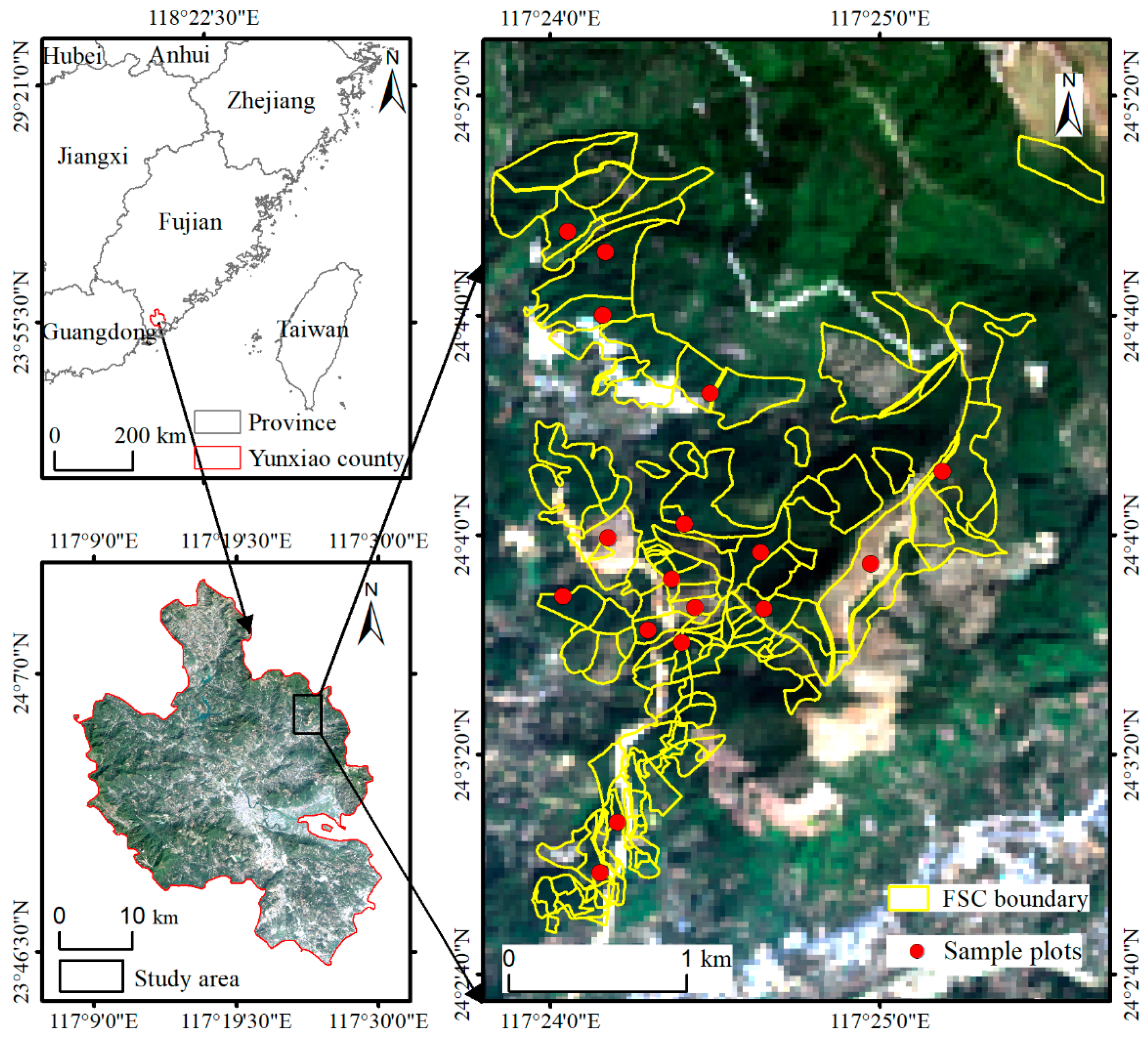
2.1. Study Area

The study area is located in Yuanling State Forestry Farm in Yunxiao County, Zhangzhou City, Fujian Province, China (Figure 1). It has a typical southern subtropical maritime monsoon climate with an average annual temperature of 21.2 °C and annual precipitation of 1730.6 mm. The planting history of the study area in recent decades can be summarized as: rubber trees was planted in the beginning of the 1980s, and were gradually replaced by fruit trees (such as longan) from 1993 due to the declined economic value of rubber trees, and eucalyptus was introduced around 2005, and then widely planted in the study area. Some Chinese fir and Pinus elliottii forests were also gradually replaced by eucalyptus during the period 2007–2010. The main species of eucalyptus were eucalyptus grandis x urophylla and eucalyptus urophylla S.T. Blake.

2.2. Data collection and Processing

2.2.1. Field Survey Data

The survey data include the FSC data carried out by government departments in 2017, and SP data surveyed in 2021. The main information of the FSC data includes average diameter at breast height (DBH), average tree height (H), stand age, survey date, stand volume per hectare, number of trees per hectare, elevation, depth of soil, etc. The FSC data were surveyed in 2017 and are the latest available forestry survey data. We chose 140 eucalyptus FSC, a total area of 379.2 ha, to carry out our simulation with the 3-PG model (Figure 1). The forest age of these FSC in 2017 was mostly concentrated in 0–4 and 9–12 years (Table 1).
We investigated 17 eucalyptus plots with an area of 20 m × 20 m in the study area. The forest age of the survey plots ranges from 1 to 13 years, the average DBH is 3.62–16.26 cm, and the average H is 4.02–19.69 m. We measured and recorded DBH and H for each tree with DBH greater than 5 cm in the plots. The planting time, management history, and environment information were also recorded through asking the owner. The model developed by [37] was used to calculate the biomass of each organ of each tree (Table 2). The biomass of each tree was summed to obtain the aboveground biomass of SP, and then converted to ACS by multiply carbon coefficient (0.4764) [37]. Considering eucalyptus has a very rapid growth rate and 3-PG model can simulate the forest structure monthly, the SP were surveyed about every six months (January 2021, July 2021, and December 2021). The data from the three surveys were used to verify the simulation accuracy of the model at the SP level. Some plots were harvested when conducting the second and third survey, and some plots were only measured for DBH. Finally, we collected a total of 44 DBH observations and 41 H observations for these plots after the three surveys.

2.2.2. Meteorology Data

We calculated monthly minimum temperature (°C), maximum temperature (°C), average temperatures (°C), and precipitation (mm) based on the hourly recorded data from 2008–2021 that were acquired from the meteorological station nearby the study area. Considering some FSC have an older forest age, the temperature and precipitation data were extended to 1997–2007 using the data provided by National Aeronautics and Space Administration (NASA). Solar radiation data from 1997 to 2021 were also acquired from the website (https://power.larc.nasa.gov/data-access-viewer/, accessed on 10 January 2022) due to a lack of local observations. These data have been proven to be accurate enough to provide reliable meteorological and solar radiation data in areas where site observations are sparse [38,39]. Compared with the data of the same year from the meteorological station, the two source data products have high consistency and can be used together for the model simulation.

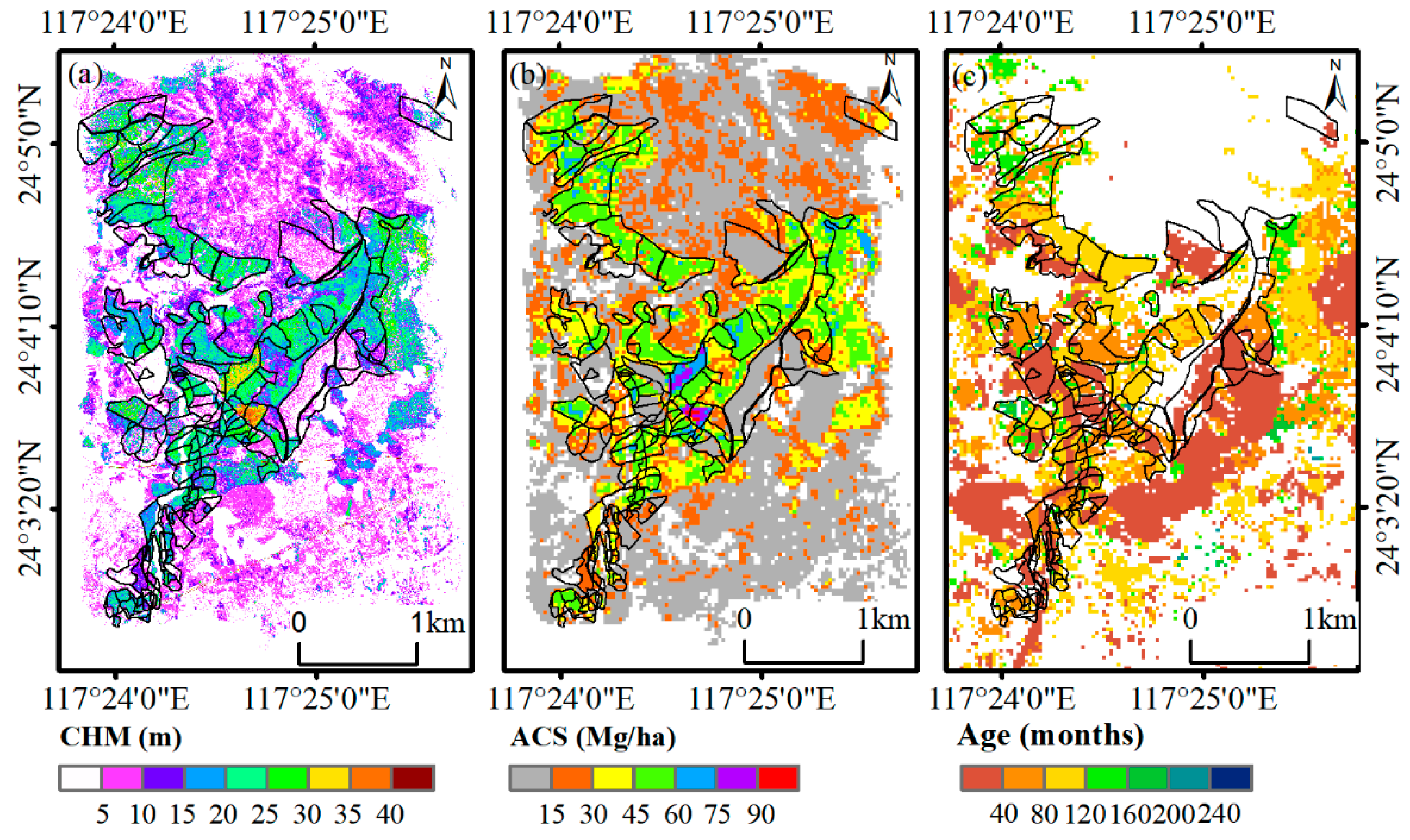
2.2.3. UAV Lidar Data

The UAV lidar data were acquired in July 2021 with an average point cloud density of 60 points/m2. The process of lidar data mainly includes filtering, denoising, normalization, and generating CHM data [40]. The Lidar360 software was used to remove noise in the point cloud data, such as bird points, low points, and utility poles. The discrete point cloud echo points were divided into ground and non-ground points. The ground points were used to generate a digital elevation model (DEM) by inverse distance weighted interpolation method. All non-ground points were interpolated to a digital surface model (DSM) with a spatial resolution of 1 m. Then, the canopy height model (CHM) was obtained by subtracting DEM from DSM. The lidar data obtained in July 2021 and sample plot data surveyed at the same time were used to establish ACS prediction model, that is, 17 observations were used in the model. Stepwise regression method was used to establish a carbon stock estimation model with the variables from the CHM acquired from lidar with a resolution of 20m × 20m (the same as plot size) [41]. Two variables (mean CHM and skewness) for ACS prediction were identified using stepwise regression method. Then, leave-one-out cross-validation was used in the evaluation processes, with 16 samples used to train the model, and the established model was used to predict the ACS value of the one observation left out of the model. The validation shows that the model works quite well, with R2 (coefficient of determination), RMSE (root mean square error), and RRMSE (relative root mean square error) values of 0.87, 8.73 Mg/ha, and 18.72%, respectively. The average H and average ACS of each FSC were calculated based on the modelled data, and used to assess the 3-PG model simulation results (Figure 2a,b).

2.2.4. Forest Age Data from Landsat Time Series Data

The forest age data of each FSC based on Landsat-based forest age data were provided by [19] (Figure 2c). The forest age of short rotation eucalyptus plantations was developed using a random localization segmentation algorithm and all available Landsat time series data. The Chow test and random forest continuous classification were used to obtain the spatial distribution of eucalyptus forest age at 30 m × 30 m spatial resolution with RMSE of 13 months in 2021. In our study area, the forest age error was about 12 months compared with the survey data. The simulation unit of this study was at FSC scale, and the average age of each FSC was obtained through zonal statistics.

2.3. 3-PG Model and Parameter Setting

The 3-PG model is a physiological–ecological process model based on allometric equations and a monthly time scale [27]. The model has a relatively simple structure and few input parameters [42]. It can simulate many tree species including eucalyptus, and is widely used in Australia, Brazil, Canada, and China [30,43,44,45]. The model was initially developed to simulate even-aged evergreen forest species, and now is able to simulate deciduous, uneven-aged, and mixed forest, and assess the forest growth under different management measures [46]. Many studies utilized the model to simulate forest growth of eucalyptus, Masson pine, and larch at the plot level [31,47,48]. The model has four submodules: the light sub-model, the biomass production and allocation sub-model, the water balance sub-model, and the mortality sub-model. More details about 3-PG model are provided in [27,45]. The tree growth was simulated at monthly intervals by inputting monthly meteorological data (maximum and minimum temperatures, average temperature, precipitation, and solar radiation), site conditions (latitude, soil class, and soil fertility), planting time, and initial organ biomass, management measures, and parameters for the tree species. The model can output many variables such as GPP, NPP, DBH, H, organ biomass (monthly), etc. The DBH, H, and ACS (calculated from biomass) were selected for output and evaluation in this study. All the simulations were performed with the r3PG package in the R platform [49].

2.3.1. Model Parameters

The 3-PG model provided a complete set of parameter values for eucalyptus, which was a very useful reference for the parameter setting of this study. For the stem biomass parameters, the key parameters aWS (0.0259) and nWS (2.8762) for eucalyptus in our study area were obtained by fitting the allometric equation WS = aWS × DBHnWS (WS is the stem biomass) (R2 = 0.9998) based on the DBH and stem biomass obtained from the survey data. The model simulation for each FSC started from its planting time, and the initialized biomass values of stem, root, and leaf were set to 1 Mg/ha, 2 Mg/ha, and 0.5 Mg/ha, respectively [50]. Soil class and soil moisture data were acquired by the Second National Soil Survey data, and other parameters were set following the reference [51]. See Appendix Table A1 for details.

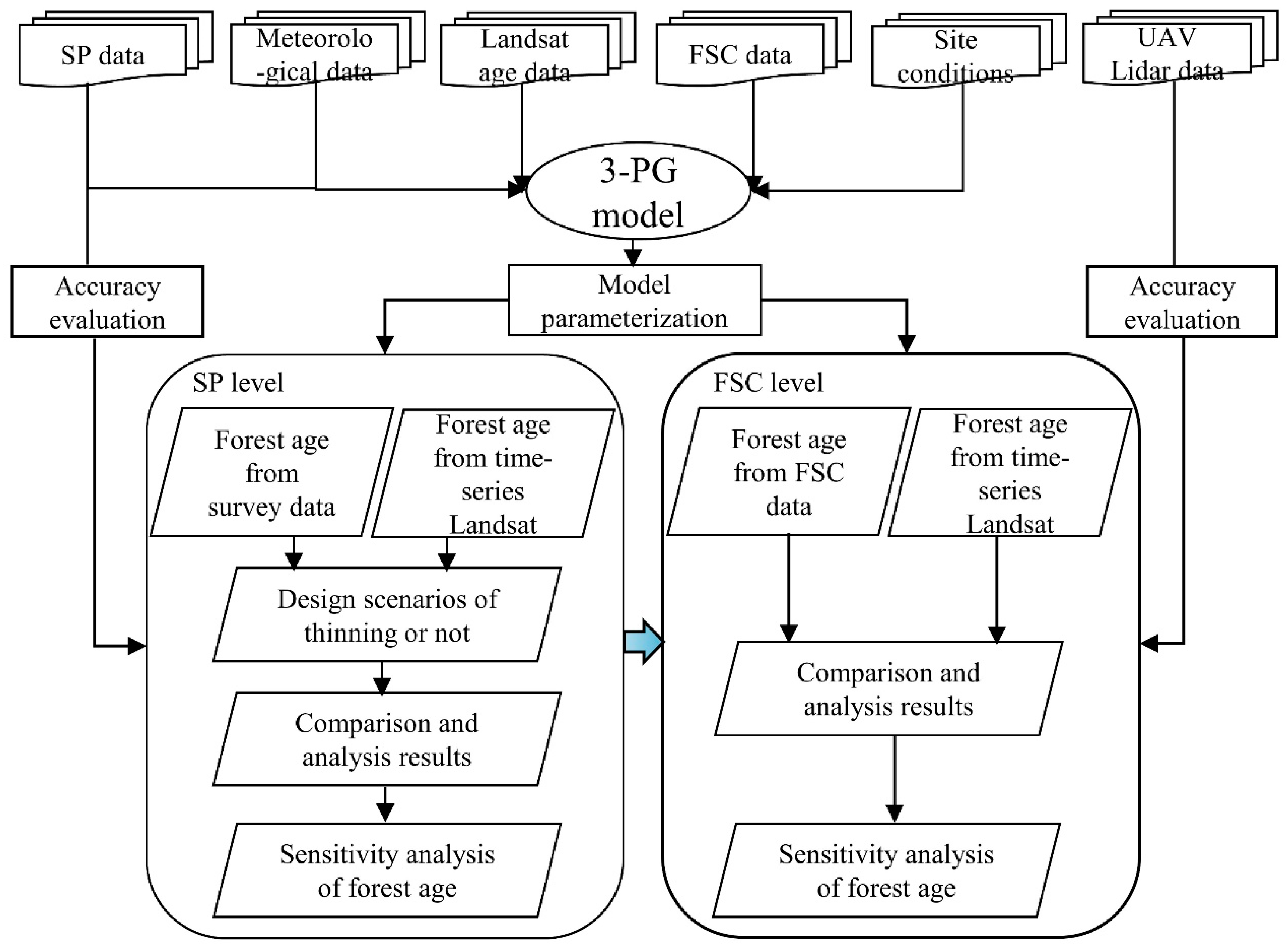
2.3.2. Simulation Scheme Design

Figure 3 shows the overall flowchart of the study. We used SP data, FSC data, Landsat age data, meteorological data, and site conditions to calibrate and drive the 3-PG model. Then, the surveyed forest age and forest age from Landsat were used to drive the 3-PG model and simulate the DBH, H, and ACS of eucalyptus plantations at the plot scale, and 17 sample plots with three sets of investigation data were used for validation. The impacts of historical management information on the accuracy of simulation results were also evaluated. Similarly, the FSC age and forest age from Landsat were used to simulate the DBH, tree height, and carbon storage of the eucalyptus plantations at the FSC scale, and validated by UAV lidar data. Finally, we explored the sensitivity of the simulated forest structure to the forest age on two scales.

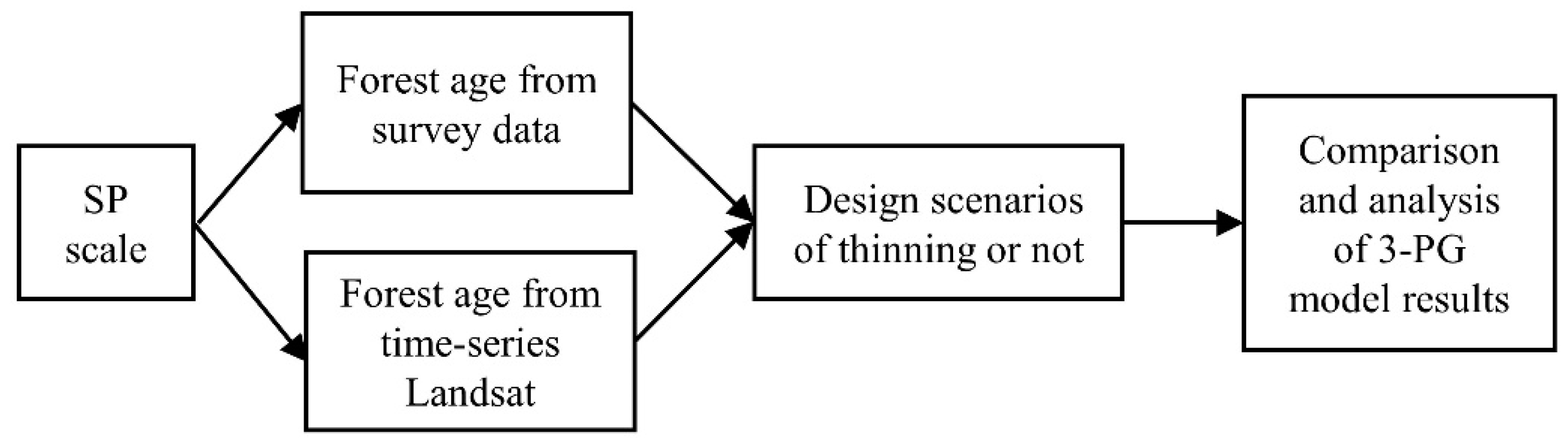
Simulation Scheme Based on the SP Level

The carbon stocks for the 17 sample plots were simulated using the parameterized 3-PG model based on the surveyed forest data and forest age data from Landsat (Figure 4). The sample plot was chosen to represent a certain area that had similar planation history and management. The forest age information of the plot was obtained by extracting the age of the pixel where the plot was located in the Landsat pixels. The impacts of historical management information on the simulation results were also evaluated by considering the selective cutting or not (acquired during the survey). It was difficult for Landsat time-series data to accurately detect the thinning activities, so the management was not considered in the forest age from Landsat-based simulation. All the biomass variables from the model were conversed to carbon stock by multiplying the carbon coefficient and obtaining the ACS. The simulation accuracy of three forest structure variables (DBH, H, ACS) were assessed by the survey data.

Simulation Scheme Based on the FSC Level

The simulations were then carried out for the 140 FSC of eucalyptus plantation. The following three scenarios were designed to evaluate the impact of forest age data on the carbon stocks simulation.
(a) Simulation based on FSC age information. The forest age from 2017 FSC survey data was used as the input data to drive the 3-PG model. Considering that FSC age was obtained from 2017, and the validation data from lidar were obtained in July 2021, some FSC may have been harvested during the period, but the FSC data may have lagged. Therefore, the FSC were divided into two groups for evaluation: FSC planted before 2015 and FSC planted after 2015 (eucalyptus plantation harvested age mainly ≥ 6 years in the study area);
(b) Simulation based on forest age data from Landsat. The forest age data (introduced in Section 2.2.3) extracted from Landsat time-series data in January 2021 were used as the input to drive the 3-PG model. It should be noted that the simulation was performed for the 140 FSC, but not for each pixel due to lack of high spatial resolution data of soil, meteorological, tree density, etc.;
(c) Simulation based on the adjusted forest age data. As the forest age based on remote sensing data has many uncertainties, we adjusted the forest age by ±3 months, ±6 months, and ±12 months to test the sensitivity of the model simulation results for both the SP and FSC.2.3.3. accuracy evaluation.
The simulated ACS, DBH, and H of SP were evaluated by the surveyed data. The simulated ACS and H of FSC were evaluated by the data calculated from UAV lidar (introduced in Section 2.2.4). The coefficient of determination (R2), root mean square error (RMSE), and relative root mean square error (RRMSE) were used to evaluate the simulation accuracy of the model. They were calculated as follows:
R 2 = i = 1 n ( y ^ i y ¯ ) 2 i = 1 n ( y i y ¯ ) 2
RMSE = i = 1 n ( y i y ^ i ) 2 n
RRMSE = i = 1 n ( y i y ^ i ) 2 n n = 1 n y i n
where n is the number of observations, y i is the observed value of plot i, y ^ i is the simulated value of plot i, and y ¯ i is the mean value of all sample plots.

3. Results

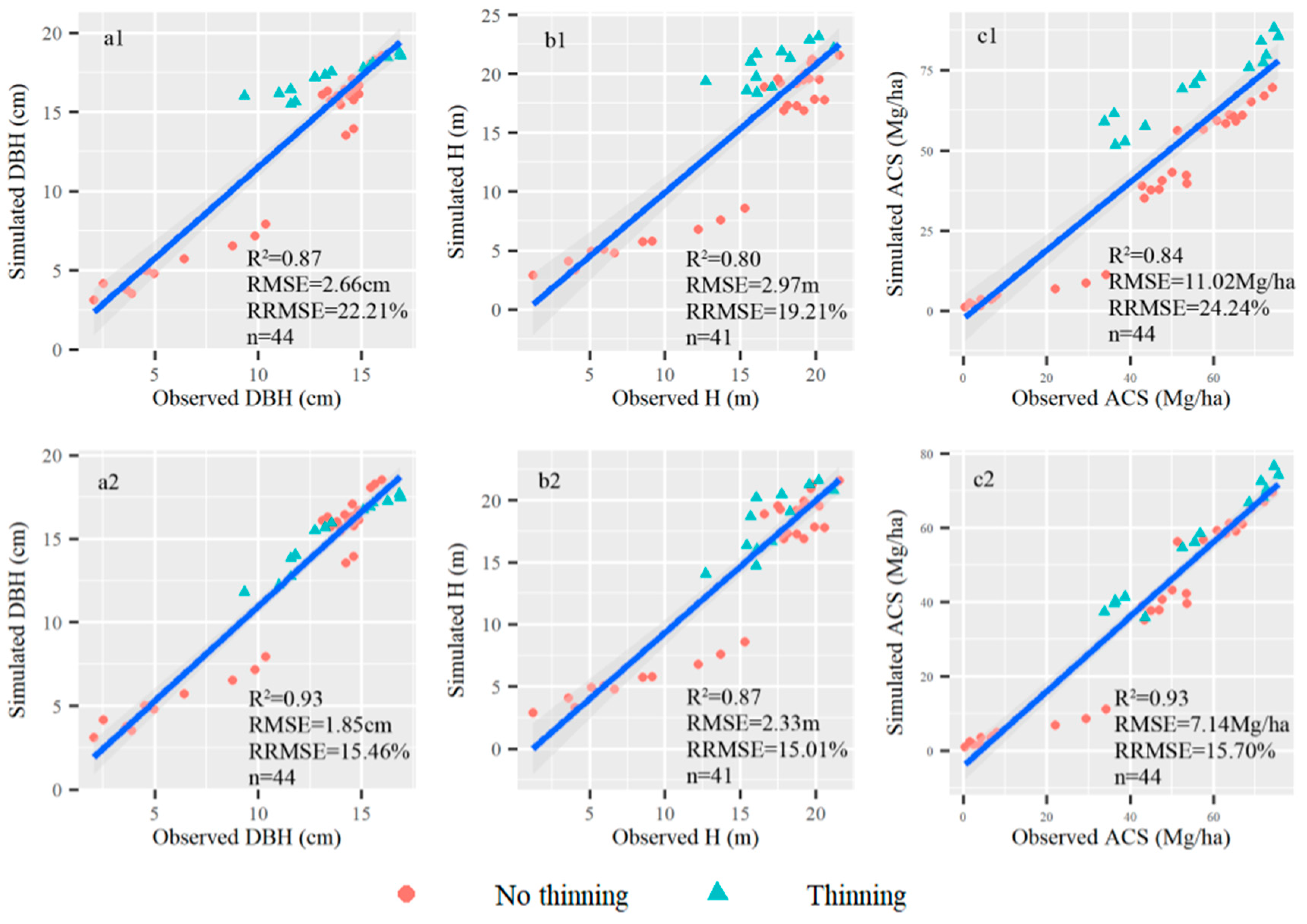
3.1. Simulation Results at SP

The results based on the surveyed forest age show that the 3-PG model can accurately simulate DBH, H, and ACS of eucalyptus plantations (Figure 5), with R2 values ranging from 0.80 to 0.93. Taking thinning information into account can further improve the simulation accuracy. The R2 of ACS, DBH, and H increase by 0.09, 0.06, and 0.07, respectively, and the RRMSE decreases by 8.54%, 6.75%, and 4.2%, respectively. The simulation results based on forest age data from Landsat also achieve high accuracy, with R2 of DBH, H, and carbon stock all higher than 0.85, and RRMSE less than 20% (Figure 6). They are generally better than the simulated results not considering thinning, and are closer to the simulated results with thinning information considered.

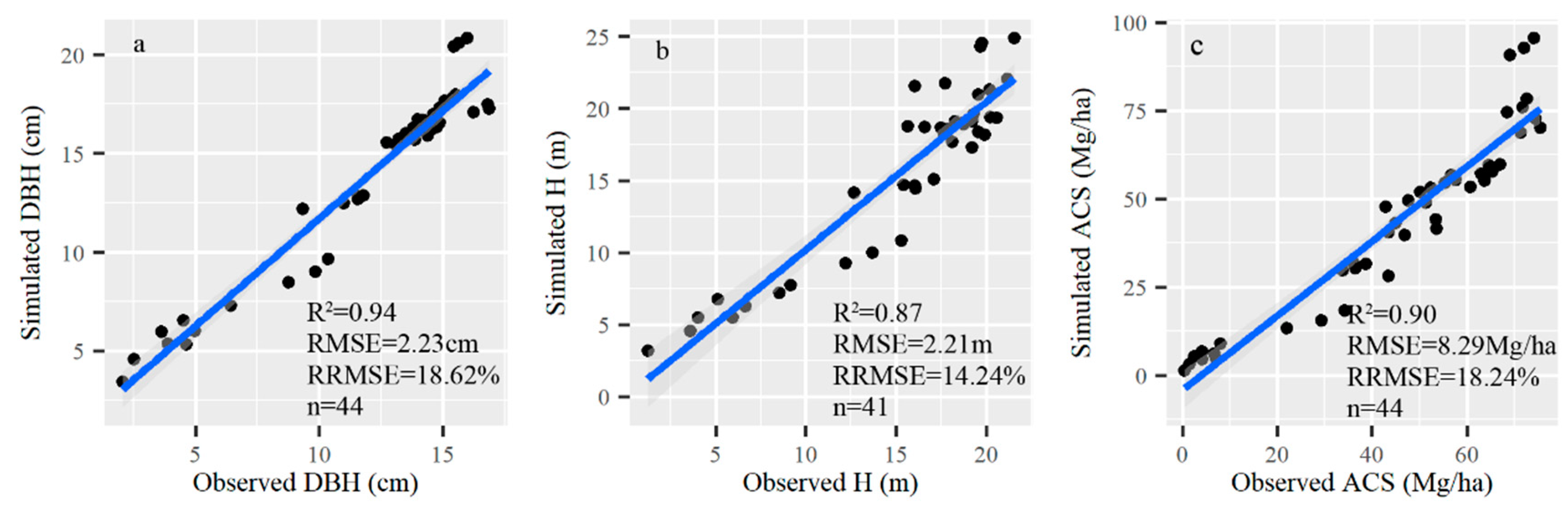
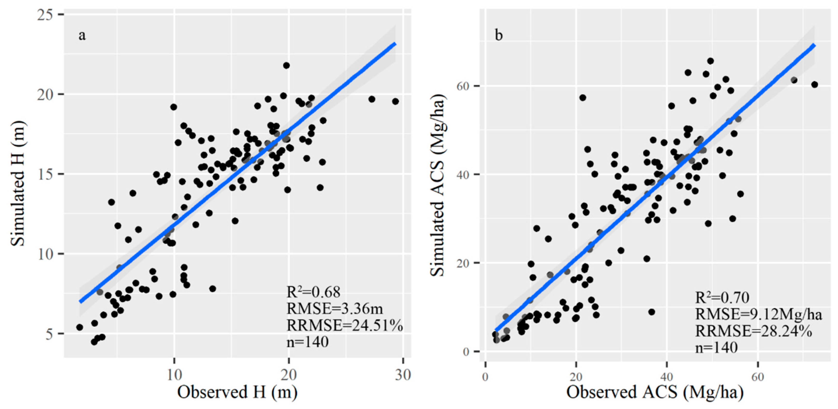
3.2. Simulation Results at FSC

The simulation results based on FSC age data for the 140 FSC show very low R2 and high RMSE compared with the ACS and H data estimated from UAV lidar. However, for the FSC planted after 2015, the simulation results are quite well-matched (Figure 7), with RMSE of H and ACS of 2.91 m and 14.22 Mg/ha, respectively. Obviously, for the FSC planted before 2015, there is no significant relationship between the simulated results and validation data, due to the unknown harvest information and inaccurate forest age data, and the RMSE of H and ACS are 14.06 m and 80.78 Mg/ha, respectively. This suggests that accurate and timely updating of forest age is critical for the model simulation of eucalyptus plantations. The accuracies of simulated H and ACS using forest age data from Landsat significantly increase for the 140 FSC compared to the results based on FSC age data (Figure 8). The forest age data from Landsat are very effective for driving the 3-PG model. Both the simulated H and ACS show high R2 and low RRMSE, but the accuracy is not so good as the SP level.

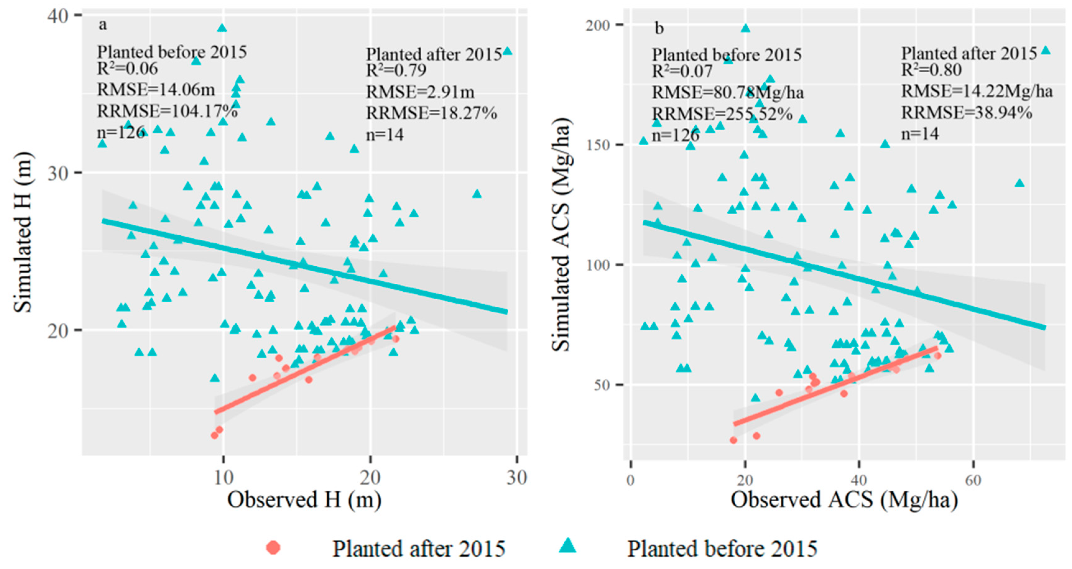
3.3. Sensitivity of the Simulation Results to Forest Age

3.3.1. Sensitivity Analysis of the 3-PG Model at the SP Level

The simulation results from different adjusted forest ages at sample plot level show that DBH, H, and ACS exhibit different degrees of variation (Table 3). The largest variation occurs in DBH with the RMSE increasing by 33.45% when the forest age increases by 12 months. The H and ACS have consistent change trends. The changes in RMSE are small when the forest age increases, but become larger when the forest age decreases from 3 months to 12 months. The RMSE of H and ACS increase by 42.92% and 82.91% as the forest age decreases 12 months. It should be noted that the sensitivity analysis shows the highest R2 and the lowest RMSE are not consistent for DBH, H, and ACS in these adjusted forest age designs. For example, the lowest RMSE of simulated DBH occurs when the forest age decreases 6 months, while for H and ACS this occurs in increased by 6 months design. In addition, the highest R2 and lowest RMSE occur in forest age adjusted designs that are inconsistent.

3.3.2. Sensitivity Analysis of the 3-PG Model at the FSC Level

The impacts of adjusted forest age on the simulated H and ACS for the 140 FSC show that the largest deviation for both occurs in the scenario of increased age of 12 months (Table 4), with RMSE increasing by 12.2% and 41.23%, respectively. The lowest RMSE of H and ACS are observed in the scenario of decreased age of 3 months and no adjustment scenario, respectively. The decreased forest age does not lead to much variation in ACS simulation at the SP level.

4. Discussion

4.1. High Accuracy Can Be Realized Based on the Forest Age Data from Landsat

The 3-PG model has been widely used to estimate forest growth parameters such as DBH, H, biomass, and NPP. In addition, the model can also output other parameters, such as forest volume, stand basal area, and stand density, which are required by forest managers. In this study, we estimated and evaluated the simulated DBH, H, and ACS of eucalyptus at the SP level and FSC level, and analyzed their sensitivity to the forest age data. During the simulation, we adopted most of the default parameters that have been established for eucalyptus (except the allometric growth equations) [51]. Both the measured data and estimated data from UAV lidar show that the 3-PG model has high simulation accuracy as long as high-quality forest age is provided. The management information can further improve the simulation accuracy. Our study shows that the forest age data from Landsat data have similar simulation accuracy with the scenario of using surveyed forest age and thinning data together. The reasons might be the uncertainties of surveyed forest age data and the minor impact of thinning measures on final ACS. In fact, it is difficult to acquire the exact planting time of eucalyptus (e.g., month), especially under the condition of the coexistence of coppice and planting. Eucalyptus has a very rapid growth in the early stage and reaches canopy closure within 2–3 years [19]. It is very difficult to obtain such high precision planting time. The forest planting time in the model was needed to be set at month, which might be difficult to simulate the early growth process of eucalyptus. The assimilation of more dense time series remote sensing data or products (e.g., LAI from Landsat or Sentinel) might improve these processes.
As an important parameter of forest carbon cycle model, forest age represents the planting time of trees/stands and reflects the current growth stage. For physiological–ecological process models, changes in stand age inevitably affect factors such as stomatal conductivity and hydraulic conductivity, which, in turn, affect physiological processes in trees, such as photosynthesis and root turnover rates [27,52]. In addition, trees at different ages have different sensitivities to parameters [53], e.g., trees have a high sensitivity to parameters such as soil fertility in the young stage and a low sensitivity to stand density in the mature stage. Therefore, it is necessary to obtain accurate and reliable information on the age of the forest during the carbon cycle, and will be the fundamental to optimize and parameterize the regional carbon models.
The constant (aWS) and power (nWS) in the allometric equation of stem biomass play an important role in the biomass allocation sub-model. Previous studies show that the main reason for the poor simulation of the 3-PG model is not using the local biomass allocation and allometric growth parameters [54]. This parameter was also observed to have the greatest influence on the simulated volume and DBH of Chinese fir in Nanping, Fujian [55]. The remaining parameters of the model can also affect the simulation accuracy of the model. For example, Hua et al. [56] found that the simulation accuracy can be further improved by fitting the maximum canopy conductance and canopy quantum efficiency based on the corrected aWS and nWS. Deciduous species have distinct growing seasons and non-growing seasons, which can be set through several parameters such as temperature, gammaF1 (maximum litterfall rate), gammaF0 (litterfall rate at t = 0), leafgrow, and leaffall. For example, for deciduous species, gammaF0 and gammaF1 can be set to 0, because all of the foliage will disappear at the end of the growing season. Eucalyptus is an evergreen tree species and previous research with 3-PG models seldom considered the difference between growing season and non-growing season [48,51,57,58]. However, further studies should pay more attention to the growth characteristics and responses to extreme climate events in different seasons.

4.2. Impact of Spatial Heterogeneity on Modelling Results

The simulated carbon stock for FSC using remote-sensing-based forest age data is significantly improved compared to the results based on FSC forest age data. However, some FSC still deviate greatly from the observed data, which is probably caused by the spatial heterogeneity of the FSC. At the beginning, the boundary of FSC was determined by the homogeneity within the forest stand, and similar management was performed. As time goes on, the same FSC might experience different management measures (thinning, fertilization, tree species, etc.) and disturbances (fires, diseases, typhoons), which causes the FSC to be more heterogeneous (for example in Figure 9). Both the CHM and aerial maps (Figure 9a1,a2) show that H in the northeast of the FSC is high, up to 30 m, but is low in the northwest of the FSC, and the maximum difference reaches 20 m. Obviously, the ACS also shows high spatial heterogeneity in this FSC. In Figure 9b, the H of the FSC is generally high, but the heterogeneity within the FSC is more obvious, and the difference between high and low trees is close to 25 m. This spatial heterogeneity could easily lead to overestimation or underestimation of the simulation results in the simulation process. Therefore, it is necessary to redraw the FSC and determine new boundaries to reduce the heterogeneity in future study, which will, potentially, significantly improve the accuracy of simulation results.

4.3. Limitations and Potential Improvement

The 3-PG model was used to estimate DBH, H, and ACS of eucalyptus based on forest age data, meteorological data, and site conditions in the study area, and obtained a high simulation accuracy. The model can not only simulate the normal growing forest, but also estimate the growth state of the forest under different management measures such as thinning. Through thinning management, forests can achieve the goal of adjusting stand density, changing stand structure, and reducing competition among individual tree species, thus, changing the normal growth of trees. The simulation results at the SP scale show that the model captured well the thinning effects on forest growth. Considering thinning information can improve the simulation accuracy, which is consistent with the research results of Xie et al. [10]. However, the response of NPP to thinning measures has not been well-explored, and positive, negative, and neutral impacts coexist in different studies [59,60,61]. This should be better considered in future simulations. Landsat time-series data-based forest age data fails to monitor management such as thinning in eucalyptus plantations due to its coarse resolution in spatial and temporal data. This may reduce the accuracy of model simulation. Therefore, these subtle changes in forest dynamics should be better characterized through spectral mixture analysis or the use of higher spatial–temporal resolution data (such as Sentinel, Gaofen).

5. Conclusions

In this study, a process-based physiological–ecological 3-PG model was used to predict the forest structure of eucalyptus plantations at the local scale by combining remotely sensed stand age data. The results show that the 3-PG model can achieve satisfactory simulation results at the SP and FSC scales. The results of sensitivity analysis show that forest age has a significant effect on forest carbon stocks, with a maximum difference of 82.91% and 41.23% in ACS between different stand age conditions at the SP scale and FSC scale, respectively. The fact that thinning information can improve the simulation accuracy, but that the information is difficult to obtain, especially for the remote sensing data, must be considered. More subtle changes can be further acquired by integrating more efficient change detection algorithms and high spatial–temporal resolution data. This study was carried out in a local forestry farm, but our method can be easily extended to large regions with the time-series remote-sensing-acquired forest age data. The impact of uncertainty in the remotely sensed forest age data provides a useful reference for regional forest carbon cycle simulations based on forest age products.

Author Contributions

Conceptualization, D.L. (Dengqiu Li) and D.L. (Dengsheng Lu); methodology, Y.Z., D.L. (Dengqiu Li) and D.L. (Dengsheng Lu); software, Y.Z.; validation, Y.Z., D.L. (Dengqiu Li), X.J. and Y.L.; formal analysis, Y.Z. and D.L. (Dengqiu Li); investigation, Y.Z., X.J., and Y.L.; resources, D.L. (Dengqiu Li) and D.L. (Dengsheng Lu); data curation, Y.Z. and D.L. (Dengqiu Li); writing—original draft preparation, Y.Z. and D.L. (Dengqiu Li); writing—review and editing, D.L. (Dengqiu Li) and D.L. (Dengsheng Lu); visualization, Y.Z. and D.L. (Dengqiu Li); supervision, D.L. (Dengqiu Li) and D.L. (Dengsheng Lu); project administration, D.L. (Dengqiu Li) and D.L. (Dengsheng Lu); funding acquisition, D.L. (Dengqiu Li) and D.L. (Dengsheng Lu). All authors have read and agreed to the published version of the manuscript.

Funding

This research was financially supported by the Natural Science Foundation of Fujian Province, grant number 2022J01640, Public welfare projects of Fujian Provincial Science and Technology Department, grant number 2021R1002008, and the National Natural Science Foundation of China, grant number 41701490.

Data Availability Statement

Due to confidentiality agreements, supporting data can only be made available to bona fide researchers subject to a non-disclosure agreement. Details of the data and how to request access are available from Professor Dengqiu Li at Fujian Normal University.

Acknowledgments

The authors thank reviewers for their help in improving our manuscript.

Conflicts of Interest

The authors declare no conflict of interest.

Appendix

Table A1. Description of parameters, unit, source, and their values.
Parameter NameDescriptionUnitSourceValue
pFS2Foliage:stem partitioning ratio at DBH = 2 cm-D1
pFS20Foliage:stem partitioning ratio at DBH = 20 cm-D0.15
aWSConstant in stem mass vs. DBH relationship-F0.0259
nWSPower in stem mass vs. DBH relationship-F2.8762
pRxMaximum fraction of NPP to roots-D0.8
pRnMinimum fraction of NPP to roots-D0.25
gammaF0Litterfall rate at t = 0 monthmonth−1D0.001
gammaF1Litterfall rate for mature standsmonth−1D0.027
tgammaFAge at which litterfall rate has median valuemonth−1D12
RttoverAverage monthly root turnover ratemonth−1D0.015
TminMinimum temperature for growthF10
ToptOptimum temperature for growthF20
TmaxMaximum temperature for growthF36
MaxAgeMaximum stand age used in age modifieryrD50
nAgePower of relative age in fage-D4
rAgeRelative age to give fage = 0.5-D0.95
MinCondMinimum canopy conductancem s−1D0
MaxCondMaximum canopy conductancem s−1D0.02
LAIgcxLAI for maximum canopy conductancem2 m−2D3.33
thinPowerPower in self-thinning rule-D1.5
SLA0Specific leaf area at age 0m2 kg−1D11
SLA1Specific leaf area for mature standsm2 kg−1D4
tSLAAge at which specific leaf area = (SLA0+SLA1)/2yrD2.5
KExtinction coefficient for absorption of PAR by canopy-D0.5
fullCanAgeAge at full canopy coveryrD3
alphaCxMaximum canopy quantum efficiency-D0.06
YRatio NPP/GPP-D0.47
fracBB0Branch and bark fraction at age 0-D0.75
fracBB1Branch and bark fraction for mature stands-D0.15
tBBAge at which pBB = 1/2(PBB0 + PBB1)yrD2
aHConstant in the stem H relationship-F1.4022
nHBPower of DBH in stem H relationship-F0.7079
nHNPower of competition in stem H relationship-F0.2492

References

  1. Pan, Y.; Chen, J.M.; Birdsey, R.; McCullough, K.; He, L.; Deng, F. Age Structure and Disturbance Legacy of North American Forests. Biogeosciences 2011, 8, 715–732. [Google Scholar] [CrossRef] [Green Version]
  2. Piao, S.; He, Y.; Wang, X.; Chen, F. Estimation of China’s Terrestrial Ecosystem Carbon Sink: Methods, Progress and Prospects. Sci. China Earth Sci. 2022, 65, 641–651. [Google Scholar] [CrossRef]
  3. Tang, S.; Tian, Q.; Xu, K.; Xu, N.; Yue, J. Age Information Retrieval of Larix Gmelinii Forest Using Sentinel-2 Data. Natl. Remote Sens. Bull. 2020, 24, 1511–1524. [Google Scholar]
  4. Koedsin, W.; Huete, A. Mapping Rubber Tree Stand Age Using Pléiades Satellite Imagery: A Case Study in Thalang District, Phuket, Thailand. Eng. J. 2015, 19, 45–56. [Google Scholar] [CrossRef] [Green Version]
  5. He, L.; Chen, J.M.; Pan, Y.; Birdsey, R.; Kattge, J. Relationships between Net Primary Productivity and Forest Stand Age in U.S. Forests. Glob. Biogeochem. Cycles 2012, 26, GB3009. [Google Scholar] [CrossRef]
  6. Haywood, A.; Stone, C. Estimating Large Area Forest Carbon Stocks-a Pragmatic Design Based Strategy. Forests 2017, 8, 99. [Google Scholar] [CrossRef] [Green Version]
  7. Ju, W.; Wang, X.; Sun, Y. Age Structure Effects on Stand Biomass and Carbon Storage Distribution of Larix Olgensis Plantation. Acta Ecol. Sin. 2011, 31, 1139–1148. [Google Scholar]
  8. Yu, Z.; Zhao, H.; Liu, S.; Zhou, G.; Fang, J.; Yu, G.; Tang, X.; Wang, W.; Yan, J.; Wang, G.; et al. Mapping Forest Type and Age in China’s Plantations. Sci. Total Environ. 2020, 744, 140790. [Google Scholar] [CrossRef]
  9. Pugh, T.A.M.; Lindeskog, M.; Smith, B.; Poulter, B.; Arneth, A.; Haverd, V.; Calle, L. Role of Forest Regrowth in Global Carbon Sink Dynamics. Proc. Natl. Acad. Sci. USA 2019, 116, 4382–4387. [Google Scholar] [CrossRef] [Green Version]
  10. Xie, Y.; Wang, H.; Lei, X. Simulation of Climate Change and Thinning Effects on Productivity of Larix Olgensis Plantations in Northeast China Using 3-PGmix Model. J. Environ. Manag. 2020, 261, 110249. [Google Scholar] [CrossRef]
  11. Zhang, Y.; Yao, Y.; Wang, X.; Liu, Y.; Piao, S. Mapping Spatial Distribution of Forest Age in China. Earth Space Sci. 2017, 4, 108–116. [Google Scholar] [CrossRef]
  12. Li, F.; Li, M.; Shi, Z.; Jiang, H.; An, J. Estimate Stand Age Distribution Based on Forest Survey and Remote Sensing Data. For. Eng. 2018, 34, 30–34. [Google Scholar] [CrossRef]
  13. Xie, X.; Wang, Q.; Dai, L.; Su, D.; Wang, X.; Qi, G.; Ye, Y. Application of China’s National Forest Continuous Inventory Database. Environ. Manag. 2011, 48, 1095–1106. [Google Scholar] [CrossRef] [PubMed]
  14. Dai, M.; Tao, Z.; Lingling, Y.; Jia, G. Spatial Pattern of Forest Ages in China Retrieved from National-Level Inventory and Remote Sensing Imageries. Geogr. Res. 2011, 30, 172–184. [Google Scholar]
  15. Zhang, C.; Ju, W.; Chen, J.; Li, D.; Wang, X.; Fan, W.; Li, M.; Zan, M. Mapping Forest Stand Age in China Using Remotely Sensed Forest Height and Observation Data. J. Geophys. Res. Biogeosci. 2014, 119, 1163–1179. [Google Scholar] [CrossRef]
  16. Besnard, S.; Koirala, S.; Santoro, M.; Weber, U.; Nelson, J.; Gütter, J.; Herault, B.; Kassi, J.; N’Guessan, A.; Neigh, C.; et al. Mapping Global Forest Age from Forest Inventories, Biomass and Climate Data. Earth Syst. Sci. Data 2021, 13, 4881–4896. [Google Scholar] [CrossRef]
  17. Ma, S.; Zhou, Z.; Zhang, Y.; An, Y.; Yang, G. Bin Identification of Forest Disturbance and Estimation of Forest Age in Subtropical Mountainous Areas Based on Landsat Time Series Data. Earth Sci. Inform. 2022, 15, 321–334. [Google Scholar] [CrossRef]
  18. Zhao, F.; Sun, R.; Zhong, L.; Meng, R.; Huang, C.; Zeng, X.; Wang, M.; Li, Y.; Wang, Z. Monthly Mapping of Forest Harvesting Using Dense Time Series Sentinel-1 SAR Imagery and Deep Learning. Remote Sens. Environ. 2022, 269, 112822. [Google Scholar] [CrossRef]
  19. Li, D.; Lu, D.; Wu, Y.; Luo, K. Retrieval of Eucalyptus Planting History and Stand Age Using Random Localization Segmentation and Continuous Land-Cover Classification Based on Landsat Time-Series Data. GISci. Remote Sens. 2022, 59, 1426–1445. [Google Scholar] [CrossRef]
  20. Zhang, Q.; Pavlic, G.; Chen, W.; Latifovic, R.; Fraser, R.; Cihlar, J. Deriving Stand Age Distribution in Boreal Forests Using SPOT VEGETATION and NOAA AVHRR Imagery. Remote Sens. Environ. 2004, 91, 405–418. [Google Scholar] [CrossRef]
  21. Spracklen, B.; Spracklen, D.V. Synergistic Use of Sentinel-1 and Sentinel-2 to Map Natural Forest and Acacia Plantation and Stand Ages in North-Central Vietnam. Remote Sens. 2021, 13, 185. [Google Scholar] [CrossRef]
  22. Pérez-Cruzado, C.; Muñoz-Sáez, F.; Basurco, F.; Riesco, G.; Rodríguez-Soalleiro, R. Combining Empirical Models and the Process-Based Model 3-PG to Predict Eucalyptus Nitens Plantations Growth in Spain. For. Ecol. Manag. 2011, 262, 1067–1077. [Google Scholar] [CrossRef]
  23. Zhao, J.; Liu, D.; Zhu, Y.; Peng, H.; Xie, H. A Review of Forest Carbon Cycle Models on Spatiotemporal Scales. J. Clean. Prod. 2022, 339, 130692. [Google Scholar] [CrossRef]
  24. Wang, P. Forest Carbon Cycle Model: A Review. Chin. J. Appl. Ecol. 2009, 20, 1505–1510. [Google Scholar]
  25. Frolking, S.; Goulden, M.L.; Wofsy, S.C.; Fan, S.M.; Sutton, D.J.; Munger, J.W.; Bazzaz, A.M.; Daube, B.C.; Crill, P.M.; Aber, J.D.; et al. Modelling Temporal Variability in the Carbon Balance of a Spruce/moss Boreal Forest. Glob. Chang. Biol. 1996, 2, 343–366. [Google Scholar] [CrossRef] [Green Version]
  26. Seidl, R.; Rammer, W.; Scheller, R.M.; Spies, T.A. An Individual-Based Process Model to Simulate Landscape-Scale Forest Ecosystem Dynamics. Ecol. Model. 2012, 231, 87–100. [Google Scholar] [CrossRef] [Green Version]
  27. Landsberg, J.J.; Waring, R.H. A Generalised Model of Forest Productivity Using Simplified Concepts of Radiation-Use Efficiency, Carbon Balance and Partitioning. For. Ecol. Manag. 1997, 95, 209–228. [Google Scholar] [CrossRef]
  28. Cai, Y.; Guan, K.; Lobell, D.; Potgieter, A.B.; Wang, S.; Peng, J.; Xu, T.; Asseng, S.; Zhang, Y.; You, L.; et al. Integrating Satellite and Climate Data to Predict Wheat Yield in Australia Using Machine Learning Approaches. Agric. For. Meteorol. 2019, 274, 144–159. [Google Scholar] [CrossRef]
  29. Seidl, R.; Rammer, W. Climate Change Amplifies the Interactions between Wind and Bark Beetle Disturbances in Forest Landscapes. Landsc. Ecol. 2017, 32, 1485–1498. [Google Scholar] [CrossRef] [Green Version]
  30. Chang, X.; Xing, Y.; Wang, X.; You, H.; Xu, K. Application of 3PG Carbon Production Model in the Gross Primary Productivity Estimation of Broadleaved Korean Pine Forest in Changbai Mountain, China. Chin. J. Appl. Ecol. 2019, 30, 1599–1607. [Google Scholar]
  31. Xie, Y.; Wang, H.; Lei, X. Application of the 3-PG Model to Predict Growth of Larix Olgensis Plantations in Northeastern China. For. Ecol. Manag. 2017, 406, 208–218. [Google Scholar] [CrossRef]
  32. Zhang, Y.X.; Wang, X.J. Geographical Spatial Distribution and Productivity Dynamic Change of Eucalyptus Plantations in China. Sci. Rep. 2021, 11, 19764. [Google Scholar] [CrossRef] [PubMed]
  33. Huang, G.; Zhao, Q. The History, Status Quo, Ecological Problems and Countermeasures of Eucalyptus Plantations in Guangxi. Acta Ecol. Sin. 2014, 34, 5142–5152. [Google Scholar] [CrossRef]
  34. Wen, Y.; Zhou, X.; Yu, S.; Zhu, H. The Predicament and Countermeasures of Development of Global Eucalyptus Plantations. Guangxi Sci. 2018, 25, 107–116, 229. [Google Scholar]
  35. Zaiton, S.; Sheriza, M.R.; Ainishifaa, R.; Alfred, K.; Norfaryanti, K. Eucalyptus in Malaysia: Review on Environmental Impacts. J. Landsc. Ecol. Repub. 2020, 13, 79–94. [Google Scholar] [CrossRef]
  36. Bayle, G.K. Ecological and Social Impacts of Eucalyptus Tree Plantation on the Environment. J. Biodivers. Conserv. Bioresour. Manag. 2019, 5, 93–104. [Google Scholar] [CrossRef]
  37. Shi, Y.; Wei, G.; Zhang, L.; Du, A. Patterns of Vegetation Carbon Storage in Eucalyptus Urophylla X E.grandis Plantations of Different Ages. Eucalypt Sci. Technol. 2017, 34, 24–27. [Google Scholar] [CrossRef]
  38. White, J.W.; Hoogenboom, G.; Wilkens, P.W.; Stackhouse, P.W.; Hoel, J.M. Evaluation of Satellite-Based, Modeled-Derived Daily Solar Radiation Data for the Continental United States. Agron. J. 2011, 103, 1242–1251. [Google Scholar] [CrossRef] [Green Version]
  39. Zhang, T.; Stackhouse, P.W.; Macpherson, B.; Mikovitz, J.C. A Solar Azimuth Formula That Renders Circumstantial Treatment Unnecessary without Compromising Mathematical Rigor: Mathematical Setup, Application and Extension of a Formula Based on the Subsolar Point and atan2 Function. Renew. Energy 2021, 172, 1333–1340. [Google Scholar] [CrossRef]
  40. Chen, Q.; Wang, X.; Hang, M.; Li, J. Research on the Improvement of Single Tree Segmentation Algorithm Based on Airborne LiDAR Point Cloud. Open Geosci. 2021, 13, 705–716. [Google Scholar] [CrossRef]
  41. Jiang, X.; Li, G.; Lu, D.; Chen, E.; Wei, X. Stratification-Based Forest Aboveground Biomass Estimation in a Subtropical Region Using Airborne Lidar Data. Remote Sens. 2020, 12, 1101. [Google Scholar] [CrossRef] [Green Version]
  42. Gupta, R.; Sharma, L.K. The Process-Based Forest Growth Model 3-PG for Use in Forest Management: A Review. Ecol. Model. 2019, 397, 55–73. [Google Scholar] [CrossRef]
  43. Grace, P.R.; Basso, B. Offsetting Greenhouse Gas Emissions through Biological Carbon Sequestration in North Eastern Australia. Agric. Syst. 2012, 105, 1–6. [Google Scholar] [CrossRef]
  44. Almeida, A.C.; Landsberg, J.J.; Sands, P.J. Parameterisation of 3-PG Model for Fast-Growing Eucalyptus Grandis Plantations. For. Ecol. Manag. 2004, 193, 179–195. [Google Scholar] [CrossRef]
  45. Jégo, G.; Thibodeau, F.; Morissette, R.; Crépeau, M.; Claessens, A.; Savoie, P. Estimating the Yield Potential of Short-Rotation Willow in Canada Using the 3PG Model. Can. J. For. Res. 2017, 47, 636–647. [Google Scholar] [CrossRef] [Green Version]
  46. Forrester, D.I.; Tang, X. Analysing the Spatial and Temporal Dynamics of Species Interactions in Mixed-Species Forests and the Effects of Stand Density Using the 3-PG Model. Ecol. Model. 2015, 319, 233–254. [Google Scholar] [CrossRef]
  47. Qu, L.H.; Zhao, X.H.; Zhang, C.Y. Application of 3-PG Model in the Prediction of Growth Factors in Natural Larix Gmelinii Forest. For. Res. 2022, 35, 158–165. [Google Scholar] [CrossRef]
  48. Elli, E.F.; Sentelhas, P.C.; de Freitas, C.H.; Carneiro, R.L.; Alvares, C.A. Assessing the Growth Gaps of Eucalyptus Plantations in Brazil–Magnitudes, Causes and Possible Mitigation Strategies. For. Ecol. Manag. 2019, 451, 117464. [Google Scholar] [CrossRef]
  49. Trotsiuk, V.; Hartig, F.; Forrester, D.I. r3PG—An R Package for Simulating Forest Growth Using the 3-PG Process-Based Model. Methods Ecol. Evol. 2020, 11, 1470–1475. [Google Scholar] [CrossRef]
  50. Wang, B.; Waters, C.; Anwar, M.R.; Cowie, A.; Liu, D.L.; Summers, D.; Paul, K.; Feng, P. Future Climate Impacts on Forest Growth and Implications for Carbon Sequestration through Reforestation in Southeast Australia. J. Environ. Manag. 2022, 302, 113964. [Google Scholar] [CrossRef]
  51. Sands, P.J.; Landsberg, J.J. Parameterisation of 3-PG for Plantation Grown Eucalyptus Globulus. For. Ecol. Manag. 2002, 163, 273–292. [Google Scholar] [CrossRef]
  52. Stape, J.L.; Ryan, M.G.; Binkley, D. Testing the Utility of the 3-PG Model for Growth of Eucalyptus Grandis X Urophylla with Natural and Manipulated Supplies of Water and Nutrients. For. Ecol. Manag. 2004, 193, 219–234. [Google Scholar] [CrossRef]
  53. Song, X.; Bryan, B.A.; Almeida, A.C.; Paul, K.I.; Zhao, G.; Ren, Y. Time-Dependent Sensitivity of a Process-Based Ecological Model. Ecol. Model. 2013, 265, 114–123. [Google Scholar] [CrossRef]
  54. Fontes, L.; Landsberg, J.; Tomé, J.; Tomé, M.; Pacheco, C.A.; Soares, P.; Araujo, C. Calibration and Testing of a Generalized Process-Based Model for Use in Portuguese Eucalyptus Plantations. Can. J. For. Res. 2006, 36, 3209–3221. [Google Scholar] [CrossRef]
  55. Liu, C.; Zheng, X.; Ren, Y. Parameter Optimization of the 3PG Model Based on Sensitivity Analysis and a Bayesian Method. Forests 2020, 11, 1369. [Google Scholar] [CrossRef]
  56. Hua, L.; Jiang, X.; He, X. Application of 3-PG Model in Eucalyptus Urophylla Plantations of Southern China. J. Beijing For. Univ. 2007, 29, 100–104. [Google Scholar] [CrossRef]
  57. Rodríguez-Suárez, J.A.; Soto, B.; Iglesias, M.L.; Diaz-Fierros, F. Application of the 3PG Forest Growth Model to a Eucalyptus Globulus Plantation in Northwest Spain. Eur. J. For. Res. 2010, 129, 573–583. [Google Scholar] [CrossRef]
  58. Caldeira, D.R.M.; Alvares, C.A.; Campoe, O.C.; Hakamada, R.E.; Guerrini, I.A.; Cegatta, Í.R.; Stape, J.L. Multisite Evaluation of the 3-PG Model for the Highest Phenotypic Plasticity Eucalyptus Clone in Brazil. For. Ecol. Manag. 2020, 462, 117989. [Google Scholar] [CrossRef]
  59. Li, R.S.; Yang, Q.P.; Zhang, W.D.; Zheng, W.H.; Chi, Y.G.; Xu, M.; Fang, Y.T.; Gessler, A.; Li, M.H.; Wang, S.L. Thinning Effect on Photosynthesis Depends on Needle Ages in a Chinese Fir (Cunninghamia Lanceolata) Plantation. Sci. Total Environ. 2017, 580, 900–906. [Google Scholar] [CrossRef]
  60. Borys, A.; Suckow, F.; Reyer, C.; Gutsch, M.; Lasch-Born, P. The Impact of Climate Change under Different Thinning Regimes on Carbon Sequestration in a German Forest District. Mitig. Adapt. Strat. Glob. Chang. 2016, 21, 861–881. [Google Scholar] [CrossRef]
  61. Sabatia, C.O.; Will, R.E.; Lynch, T.B. Effect of Thinning on Aboveground Biomass Accumulation and Distribution in Naturally Regenerated Shortleaf Pine. South. J. Appl. For. 2009, 33, 188–192. [Google Scholar] [CrossRef]
Figure 1. Location of the study area, spatial distribution of sample plots, and forest sub-compartment of eucalyptus. The base map is a true color composite of Sentinel-2 image.
Remotesensing 15 00183 g001
Figure 2. CHM (a), aboveground carbon stocks (b) based on UAV lidar, and forest age data (c) from Landsat time-series data.
Remotesensing 15 00183 g002
Figure 3. The overall work flow chart of the article.
Remotesensing 15 00183 g003
Figure 4. Simulation scheme design at the sample plot level.
Remotesensing 15 00183 g004
Figure 5. Validation of simulated forest structure at the SP. Plots (a1c1) are simulated diameter at breast height, height, aboveground carbon stock of not considering thinning in the model; (a2c2) are simulated diameter at breast height, height, aboveground carbon stock of considering thinning. No thinning and thinning denote whether the SP thinned or not during the growth.
Remotesensing 15 00183 g005
Figure 6. Validation of simulated diameter at breast height (a), height (b), and aboveground carbon stock (c) based on remote sensing stand age data at SP scale.
Remotesensing 15 00183 g006
Figure 7. Validation of simulated height (a) and aboveground carbon stocks (b) based on FSC forest age data.
Remotesensing 15 00183 g007
Figure 8. Validation of simulated height (a) and aboveground carbon stocks (b) based on forest age data from Landsat.
Remotesensing 15 00183 g008
Figure 9. Spatial heterogeneity in FSC. Plots (a1,b1) are CHM; (a2,b2) are aerial photo; (a3,b3) are aboveground carbon stocks (ACS) estimated by UAV lidar data with the spatial resolution of 20 m.
Remotesensing 15 00183 g009
Table 1. Basic information of the 140 eucalyptus FSC.
Age (Year)Number (n)Mean DBH (cm)Mean H (m)Total Area (ha)
≤455<9.52.5–10.8105.38
5–82610.9–17.612.3–22115.75
9–125311.5–24.414.3–29.2143.25
13–17620.8–24.621.7–28.314.82
Total1400–27.62.5–29.2379.2
Table 2. Model for estimating aboveground biomass (stem, branch, bark, and foliage) of eucalyptus.
OrganFitting EquationR2
StemW = 0.0259 × DBH2.87620.978
BranchW = 0.0263 × DBH2.24710.887
BarkW = 0.0539 × DBH1.78020.949
FoliageW = 0.1785 × DBH1.17530.871
Table 3. Comparison of model predictions of the diameter at breast height (DBH), height (H), and aboveground carbon stocks (ACS) with observations of DBH, H, and ACS under different adjusted forest ages based at SP level.
VariablesDBHHACS
R2RMSE
(cm)
Change Degree of RMSER2RMSE
(m)
Change Degree of RMSER2RMSE
(Mg/ha)
Change Degree of RMSE
−3 months0.941.745.95%0.862.507.30%0.948.0713.03%
−6 months0.931.689.19%0.852.7718.88%0.939.5633.89%
−12 months0.901.727.03%0.793.3342.92%0.9013.0682.91%
No change0.931.8500.872.3300.937.140
+3 months0.942.0912.97%0.872.263%0.946.1513.86%
+6 months0.942.2923.78%0.872.253.43%0.955.9217.09%
+12 months0.942.7833.45%0.882.423.86%0.957.413.78%
Table 4. Comparison of model predicted height (H) and aboveground carbon stocks (ACS) with lidar inverse H and ACS under different stand age conditions based on FSC scale.
VariablesH ACS
R2RMSE (m)Change Degree of RMSER2RMSE (Mg/ha)Change Degree of RMSE
−3 months0.743.04−10.53%0.759.221.1%
−6 months0.733.04−10.53%0.749.271.64%
−12 months0.723.195.06%0.7110.3313.27%
No change0.683.3600.709.120
+3 months0.743.25−3.27%0.7710.2512.39%
+6 months0.743.41.19%0.771120.61%
+12 months0.743.7712.2%0.7712.8841.23%
Disclaimer/Publisher’s Note: The statements, opinions and data contained in all publications are solely those of the individual author(s) and contributor(s) and not of MDPI and/or the editor(s). MDPI and/or the editor(s) disclaim responsibility for any injury to people or property resulting from any ideas, methods, instructions or products referred to in the content.

