Article

Comparison of Canopy Clumping Index Measuring Methods and Analysis of Their Impact

1
School of Forestry, Northeast Forestry University, Harbin 150040, China
2
Key Laboratory of Sustainable Forest Ecosystem Management-Ministry of Education, Northeast Forestry University, Harbin 150040, China
*
Author to whom correspondence should be addressed.
Remote Sens. 2023, 15(2), 471; https://doi.org/10.3390/rs15020471
Submission received: 9 December 2022 / Revised: 4 January 2023 / Accepted: 11 January 2023 / Published: 13 January 2023
(This article belongs to the Special Issue Monitoring Forest Carbon Sequestration with Remote Sensing)

Abstract

:
The clumping index (CI) is a commonly used vegetation dispersion parameter used to characterize the spatial distribution of the clumping or random distribution of leaves in canopy environments, as well as to determine the radiation transfer of the canopy, the photosynthesis of the foliage, and hydrological processes. However, the method of CI estimation using the measurement instrument produces uncertain values in various forest types. Therefore, it is necessary to clarify the differences in CI estimation methods using field measurements with various segment lengths in different forest types. In this study, three 100 m × 100 m plots were set, and the CI and leaf area index (LAI) values were measured. The CI estimation results were compared. The results show that the accuracy of CI estimation was affected by different forest types, different stand densities, and various segment lengths. The segment length had a significant effect on CI estimation with various methods. The CI estimation accuracy of the LX and CLX methods increased alongside a decrease in the segment length. The CI evidently offered spatial heterogeneity among the different plots. Compared with the true CI, there were significant differences in the CI estimation values with the use of various methods. Moreover, the spatial distribution of the CI estimation values using the ΩCMN method could more effectively describe the spatial heterogeneity of the CI. These results can provide a reference for CI estimation in field measurements with various segment lengths in different forest types.

Graphical Abstract

1. Introduction

As a common phenomenon in natural forests, canopy clumping can affect both gap fraction and canopy radiation transfer [1,2,3]. Meanwhile, it can cause the leaf area index (LAI) to be underestimated without considering canopy clumping [4,5,6]. Therefore, it is essential to quantify the non-random distribution characteristics of the forest canopy [7].
The canopy clumping index (CI) is a commonly used vegetation dispersion parameter used to characterize the spatial distribution of leaves or needles within the forest canopy [8]. The CI is often defined as the ratio of the effective leaf area index (LAIe) to the real leaf area index (LAIr) [9]. The LAIr is defined as the total area of plant leaves per unit land area, accounting for half of the land area [10,11]. The non-randomness level of foliage distribution in the forest canopy can be quantified by the CI in real scenarios. The CI is equal to 1.0; there is a random distribution of foliage in canopy environments, i.e., larger than 1.0 when the canopy offers a regular distribution and less than 1.0 when the canopy offers an aggregated distribution [12]. An exploration into the canopy clumping effect can not only help improve understanding around canopy efficiency in order to intercept light, but can also quantitatively calculate the carbon capture of vegetation in the ecosystem and the proportion of chlorophyll fluorescence photons escaping from the canopy [13]. Therefore, accurately acquisitioning the CI is of great importance in order to understand the distribution characteristics of leaves in the canopy and gas exchange in the ecosystem [14]. Meanwhile, a lack of consideration of the CI can lead to an LAI error of up to 70% [15]. Therefore, it is essential to correctly estimate the LAI when using an indirect optical approach that accounts for the clumping effect [16].
The current CI is a ratio of the canopy gap fraction under real and random conditions, and it is a quantified ratio of the effective leaf area index (LAIe) to the real leaf area index (LAIr). In many studies, the CI is used to efficiently quantify the transmittance and interception of light and precipitation in canopy environments. Furthermore, the primary ways of obtaining the CI include field and remote sensing methods. In field measurements, the CI can be estimated both directly or indirectly using commercial optical instruments [16,17]. There are usually two steps available to retrieve the forest canopy clumping index, including the gap size estimation phase and the CI estimation phase [7]. The gap size distributions can be obtained using commercial optical instruments, such as tracing radiation and architecture of canopy (TRAC) and digital hemispherical photography (DHP) in-field measurements. For the CI estimation phase, there are several well-developed and accepted methods used to quantitatively calculate the clumping degree. The finite-length averaging method (LX) proposed by Lang and Xiang was the earliest method used for CI estimation [18]. In this method, the whole scene was divided into different segments according to the clustering effect of the whole scene, and the canopy was assumed as random distributions in each segment. The LAIr in each segment was calculated by the gap rate model and the LAIe of the whole scene was calculated by the gap rate model. Then, the CI was calculated by the ratio of the LAIe to the LAIr. Evidently, the size of the segments using this method will significantly affect the accuracy of CI estimation [19,20]. Chen et al. proposed a gap size distribution model that can be used to calculate the CI. In this method, large gaps from the measured gap size accumulation curve were sequentially removed until the pattern of gap size accumulation resembled a random spatial distribution, and the CI was calculated using the logarithmic gap size averaging method (the CC method) [21,22,23]. Unlike the LX method, this method is not limited by light conditions and has strong applicability [17]. Additionally, this method is more commonly used for CI estimation [24]. Pisek et al. improved the CC method for CI estimation based on the original Miller’s law, known as the CMN method. The difference between the CMN and CC methods is that the CMN method does not consider the normalization after removing large gaps [19]. Leblanc combined the LX and CC methods to calculate the CI from hemispheric photography (HP) images, in what is called the CLX method [25]. As a combination of the two methods, the CLX method was disadvantageous. It was sensitive to the segment length (similar to the LX method) and failed to identify and eliminate small gaps, which caused increases in the CI estimation error (similar to the CC method) [26]. To conclude, the advantages and disadvantages of various methods in different scenes are still important to consider when taking actual measurements.
In field measurements, the CI can also be estimated by obtaining the LAIe and LAIr and then calculating the ratio, which can retrieve the CI. The LAIr generally adopts destructive sampling [27], allometric growth [28], and litter collection [29]. The destructive sampling method is used to pick leaves of all vegetation in the study area and individually measure the leaf areas, before then calculating the LAIr. This method has certain impacts on the ecological environment, making it unsuitable for forests with complex structures [30]. The allometric technique depends on the relationship between the leaf area and any dimension of the element of the woody plant, such as the green leaf biomass, the stem diameter, the diameter at breast height, the tree height, or the volume [8]. Moreover, this relationship is determined via destructive sampling. The allometric equation can be used to estimate the LAIr within the study area. However, this method is disadvantageous given that it can destroy the samples. The allometric equation is also restricted because of its site specificity, and the relationship is stand-specific and dependent on the season, site fertility, local climate, and canopy structure [31,32]. The measured result may be less than the LAI, as measured by the optical instrument method [33]. The litter collection method retrieves fallen leaves during the leaf-falling period using litter traps in the study area and the LAIr can be determined from the litter using the weight method. This method is very useful for LAIr measurements, especially in deciduous forests. The accuracy of LAIr measurements was 95% within a bias of 10% with respect to the mean with an appropriate spatial and temporal sampling scheme [34,35]. The LAIe is generally measured with an optical instrument, such as Demon, LAI-2200, TRAC, SunScan, and AccuPAR, or with digital hemispheric photography (DHP). These optical instruments have usually been used to monitor the LAI status and any small-scale dynamic changes in forest ecosystems [36,37,38]. Denmon is an instrument used for log-averaging the transmittance of solar beams, and its sensor has a filter that can have a filtering effect on other scattered light measurements and can allow the light to be measured at a wavelength of only 430 nm. However, it required several repeated time observations and there were more complex operating procedures compared with LAI-2200 [8]. The LAI-2200 instrument, equipped with a fisheye lens and five concentric conical rings (7°, 23°, 38°, 53°, and 68°), was used to record incident light intensities. Similar to Denmon, the LAI-2200 calculated the LAIe by comparing the different measurements among the above and below canopies. The result measured with the LAI-2200 was usually sensitive to different light conditions, so it was used often to take measurements before dawn or after dusk [39]. The LAI-2200 has been successfully used to estimate LAIe in continuous and homogeneous canopies; however, the potential of the LAI-2200 instrument is restricted by a general tendency of LAIe underestimation [6,16]. The TRAC technique can also be used to calculate the LAI by combining the average leaf width, the needle cluster ratio, and the woody leaf area ratio of the study area [21,23]. SunScan and AccuPAR were used to calculate the LAI by measuring the solar transmittance of the upper and lower parts of the canopy, but these two methods were not suitable for measurements within coniferous forests [8]. The DHP method generally uses a fisheye lens and a digital camera to measure the canopy gap ratio and the LAI. However, the accuracy of this method depended on recognizing the algorithm of the gap ratio and woody parts, meaning that the accuracy could be further improved by the optimization algorithm [17]. To summarize, the accuracy of LAI measurements varied among different instruments, as did CI estimation when using the ratio of the LAIe and the LAIr.
Global- and regional-scale CI estimation methods have been generated by remote sensing technology. Optical remote sensing, such as with POLDER, MODIS, and MISR satellite data, has been successfully used for CI estimation purposes [40,41,42]. An empirical relationship between the CI and vegetation index, such as the normalized difference between the hotspot and dark-spot (NDHD) models, was established to obtain a clumping index [43]. Chen et al. (2005) generated a monthly CI global mapping model from POLDER with a 6 km resolution [44]. He et al. proposed a global CI mapping model based on the NDHD model at a 500 m resolution by utilizing the MODIS BRDF product [40]. Fang et al. obtained the global CI distribution data from 2000 to 2020 by calculating the NDHD based on MODIS data and implemented the retrieval service in Google Earth Engine. The results indicate that the global clumping index range is about 0.3–1.0 [45]. With the development of laser ranging technology, light detection and ranging (LiDAR) data have been used to estimate the CI through calculating the gap rate or gap fraction by CC, CLX, or other methods [7,46,47]. Unfortunately, there is no effective and robustness algorithm used to retrieve the clumping index in a wide range with spaceborne lidar. Therefore, optical remote sensing is still the primary data source for CI estimation on the large spatial and multi-temporal scale [16].
Regardless of field measurements or remote sensing estimations, accurately measuring the CI is essential. Some studies have focused on researching the availability and accuracy of CI calculation methods in field measurements [17,19,48]. The first factor that will have a potential impact on the measurement results is the segment length. Segment length is an artificially assumed variable used to estimate the CI. Before CI estimation, a cell that is small enough for the assumption of leaf distribution randomness within a cell should be assumed. Meanwhile, the size of this cell should be large enough so that the statistics of the gap fraction are meaningful. Moreover, this segment size is usually called the segment length. A theoretical analysis of this problem suggests that the segment length should be at least 10 times the width of a leaf [16]. However, varied segment lengths can lead to different and random canopy situations within each segment. In the case of relatively long segments, the canopy may have a clustered distribution. This results in a large error caused by the calculation method [17]. Leblanc et al. compared the differences in CI estimation methods and showed that the CLX method was less sensitive to the segment length compared to other methods, and the LX method was more sensitive compared with other methods [26]. Pisek et al. compared the CI estimation results using the LX method and the CLX method under various segment lengths, and showed that the segment length can have an uncertain impact on CI estimation, though the optimal segment length for CI estimation was not determined [19]. Woodgate found that the CLX method was better than the CC and LX methods for CI estimation in eucalyptus forests [49]. However, Pisek et al. found that the CLX method was more suitable for CI estimation than the CC, LX, and CMN methods in Scots pine forests [19]. This indicates that the various types of forest will increase the uncertainty of CI measurements [50]. Therefore, it is necessary to evaluate the differences in CI estimation methods when taking in-field measurements with various segment lengths in different forest types.
To sum up, the studies on the differences among CI field measuring methods were insufficient and the influence of the segment lengths, different forest types, and tree density in the plot on CI field measurement was also not clear. To this aim, three 100 × 100 m plots of different forest types were set in the research region, and the CI was estimated using the measurements from TRAC, LAI-2200, DHP, and litter collection methods. Then, the CI estimation results were compared and the uncertainty of CI estimation was analyzed at various segment lengths with the LX, CC, CLX, P, and CMN methods. These results could provide a reference for CI estimation in field measurements with various segment lengths in different forest types.

2. Materials and Methods

2.1. Study Area

The research area is located in Maoer Mountain Experimental Forest Farm of Northeast Forestry University in Shangzhi City, Heilongjiang Province, northeast of China, with longitude of 127°29′–127°44′E and a latitude of 45°14′–45°29′N (Figure 1). The area of the Maoer Mountain forest farm is about 26.496 km2. The study area is a low-mountain and hilly area with an average altitude of 300 m. The research region has a mid-temperate continental monsoon climate with an average annual temperature of 2.7 °C [51]. The hottest month is in July with an average temperature of 21.8 °C. The coldest month is in January with an average temperature of −19.9 °C [52]. The average annual precipitation is 700–800 mm.
The vegetation type of the Maoer Mountain Experimental Forest Farm is mainly natural secondary forest and artificial forest. The average forest coverage rate is 95%, and the total forest volume is 3.5 million m3. The main tree species are Quercus mongolica Fisch., Betula platyphylla Suk., Pinus koraiensis Sieb., Fraxinus mandschurica Rupr., Phellodendron amurense Rupr., Populus davidiana Dode, Tilia amurensis Rupr., Larix gmelini Rupr., and Betula costata Trautv. [52,53].

2.2. Field Data

2.2.1. Field Measurement

In this study, three 100 m × 100 m plots with different forest types were set. In order to minimize the uncertain error caused by terrain, the three selected plots were set at the region with a flat slope. These were broad-leaved forest, coniferous forest, and mixed forest plots. The measured forest parameters included the diameter at breast height (DBH), the tree height, the tree density, the tree species, the relative dominance, and the specific leaf area (SLA). The DBH above 5 cm was measured and recorded. Then, the geographical coordinate of each tree in one plot was recorded using the SOUTH RTK (SOUTH Inc., Guangzhou, China) instrument.
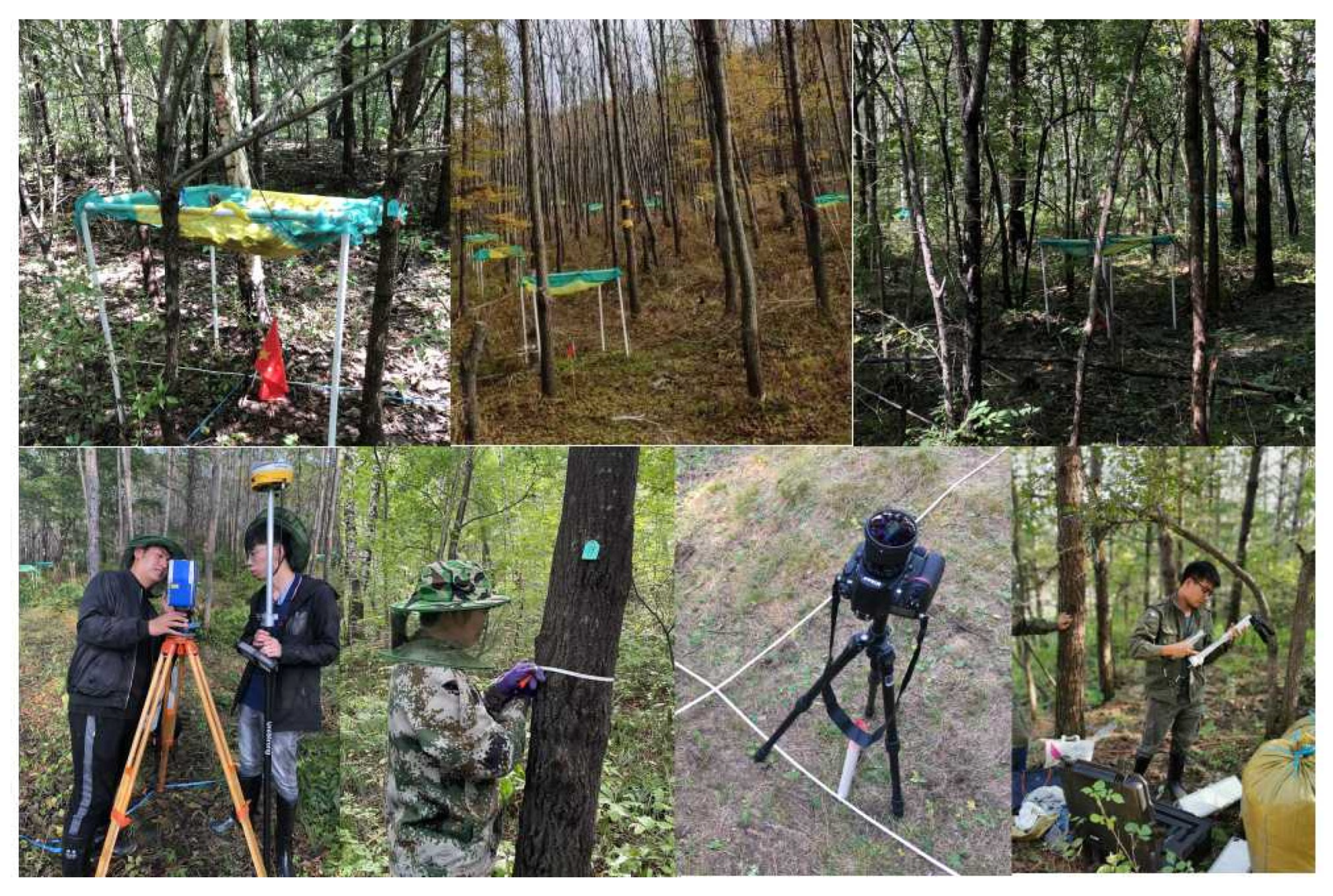
The plot was divided into 100 squares with an area of 10 m × 10 m. Moreover, a 1 m × 1 m litter trap was set at the center of each square (Figure 2). The leaves were then collected twice in each month from the beginning of the season to the end of the season. Afterwards, the area and the weight of the fresh leaves were measured. The Li-3000 was used to measure the leaf area of the deciduous tree species. Then, the needle surface area of the coniferous trees was measured using the volume displacement method, as reported in Chen’s publication in 1996 [54]. All fresh leaf samples were separated by species type and were subsequently oven-dried at 70 °C for 24 h. The mass of the dried leaf samples was recorded. The specific leaf area (SLA) was then calculated as follows [55]:
S L A = S a W
where S a is the average fresh leaf area (cm2) and W is the dried weight of leaves (g). The statistical information of the measurements can be found in Table 1.
Leaves collected from the litter trap were separated by species type and the wet weight was measured and recorded. Then, the samples were oven-dried at 70 °C for 24 h and the weights of the samples were measured. This drying process was repeated until the measured weight of the samples was less than 0.01 g. Subsequently, the ratio of leaf dry mass to fresh mass was calculated based on the measured dry and wet weight of samples, following Equation (2):
a = M 0 M 1
where M0 is the dried weight of leaf samples with a unit of g, M1 is the wet weight of leaves with a unit of g, and a is the ratio of leaf dry mass to fresh mass. This calculation was made based on the types of tree species and varied with different types of tree species.
After that, the real leaf area index of each type of tree species in the plot could be calculated based on the specific leaf area and the ratio of dry weight to fresh weight using litter collection method. The equation used to calculate the LAI was as follows:
L A I l i t t e r = a M S L A
where LAIlitter is the real leaf area index (cm2/cm2), a is the ratio of dry to fresh mass (g), M is the wet weight of the samples (g), and SLA is the specific leaf area (cm2/g). With this method, we could obtain the LAIr of each litter trap, each tree species in one plot, and the total LAIr in the plot for further analysis.

2.2.2. Measurements of the LAIe and the CI

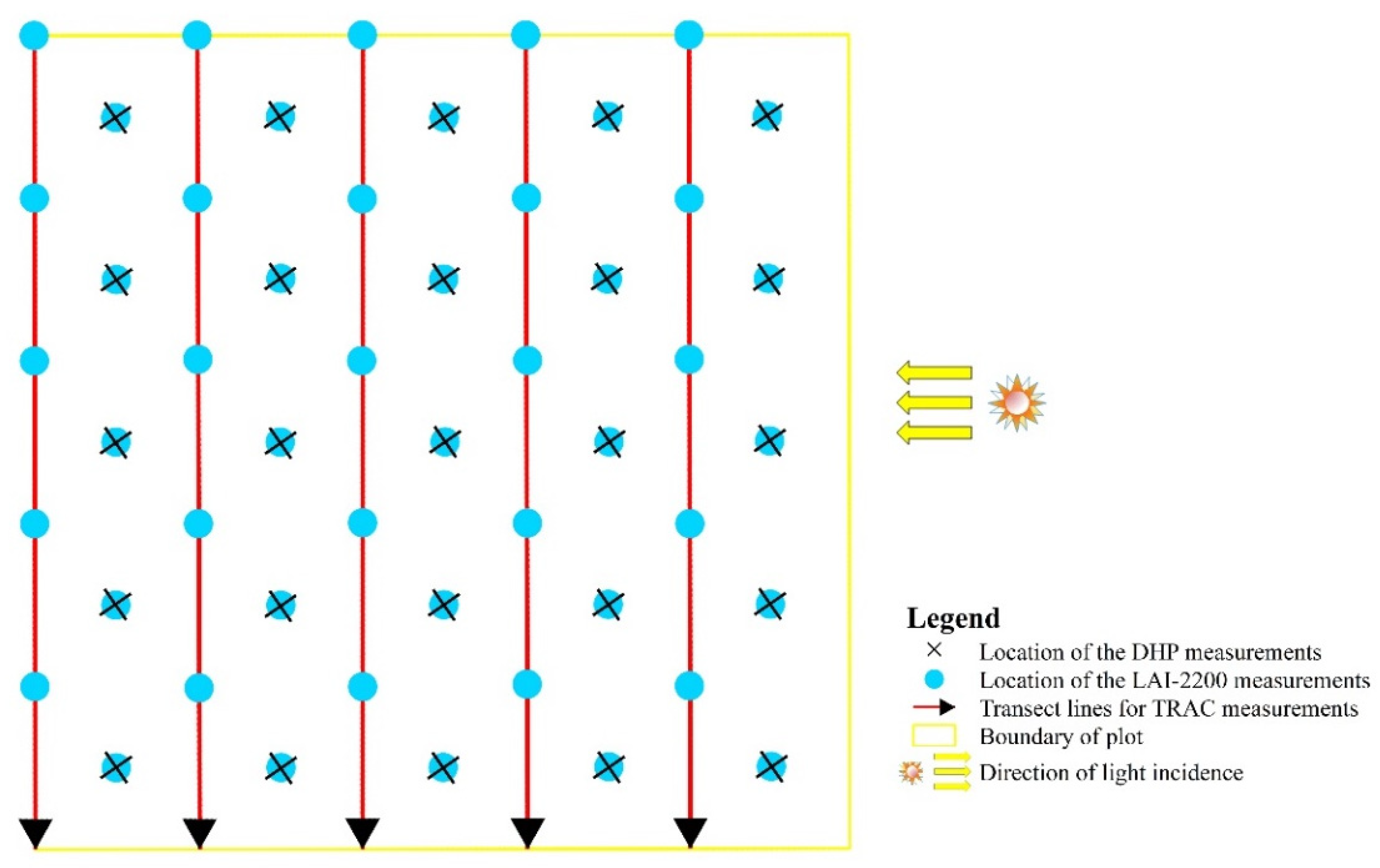
The LAIe and the CI were measured using the LAI-2200, TRAC, and DHP methods. Two pieces of LAI-2200 (LI-COR Inc., Lincoln, Nebraska, USA) equipment were used to record the light penetration into the canopy and the above canopy; as a result, the LAIe could be calculated. Each measurement was repeated twice and a 90° view cap was used to shield the sensor from the operator during the measurement stage. The measurements were conducted near sunset or under overcast conditions. It was used to minimize the measuring error under direct illumination [56]. The position of the measured LAI can be found in Figure 3.
The DHP images were taken with a fixed azimuth angle using Nikon D800 (Nikon, Tokyo, Japan) with a 4.5 mm F2.8 EX DC circular fisheye converter. The position of the DHP measurement can be found in Figure 3. The equipment was mounted and levelled using a bubble level before the measurements were taken. Then, the hemispherical photographs were taken. The effective LAI could be derived using digital hemispherical photography (DHP) software (Natural Resources Canada, Ottawa, Canada). The measurements were conducted under overcast conditions or the conditions of diffuse skylight were used to minimize the error of the direct illumination. More details can be found in the Digital Hemispherical Photography Manual [57].
The TRAC equipment was used to record the photosynthetic photon flux density (PPFD) and to retrieve the CI of the forest canopy. In this study, five transect lines of 100 m, with an interval distance of 20 m, were set. Then, we collected the TRAC-based PPFD gradient values along the line transects, which are perpendicular to the incident directions of the solar beams in the plot. To compare the differences in the results with various segment lengths, the segment lengths for TRAC measurements were set to 1 m, 2 m, 4 m, 5 m, 10 m, 20 m, 50 m, and 100 m, respectively. It helped us to create different datasets based on the original TRAC data when transects were segmented by 1 m, 2 m, 4 m, 5 m, 10 m, 20 m, 50 m, 100 m, respectively. At last, the forest canopy CI was computed using the TRACWin software (Natural Resources Canada, Ottawa, ON, Canada). To minimize the influence of the different zenith angles on the CI measurements, a zenith angle of 57.5° was used during the measurement stage [56,57,58].

2.3. Methodology of CI Estimation

In this study, we compared the CI estimation performances using the LX, P, CC, CMN, and CLX methods. Moreover, the theory of these methods is described as follows.

2.3.1. Theory of the LX Method

The LX method was the first method used for LAI estimation, which took the logarithmic averages with a solid statistical background [25]. Thus, LAI estimation can have greater accuracy when the canopy transmittance is logarithmically averaged in a discontinuous or clumped canopy, referred to as method of LX. The LX method assumed that the foliage within the finite length was random and that the segment contained gaps.
Ω LX ( θ ) = ln [ P ( θ ) ¯ ] ln [ P ( θ ) ] ¯
where P ( θ ) ¯ is the average of the canopy gap fraction and ln [ P ( θ ) ] ¯ is the logarithmic mean gap fractions for all segments. This method may give erroneous results due to the short length of the segments in a clumped canopy [59,60]. The short length of the segments is also called segment length, and is defined as the various lengths of all the sunlit segments occurring along this line that can be expressed as a statistical distribution function under given canopy [61]. In addition, the segment length is considered an essential factor for CI estimation [62].

2.3.2. Theory of the P method

The p method is based on the gap size distribution [63]. The gap size distribution of the canopy with a random canopy spatial distribution can be described as follows:
P ( ι ) = e L P ( 1 + ι w e p )
where P ( ι ) is the probability that a probe with length ι will completely fall into a light spot. w e p is the mean width of the element shadows cast on the transect. L P is the projected foliage element area.
The P ( l ) for the clumped canopy can be determined with the following formula:
P ( l ) = P c ( l ) + P E 1 ( l ) P c 1 + P E 2 ( l ) P c 2 + + P E n ( l ) P c n = P c ( l ) + i = 1 n P E i ( l ) P c i
The term P c ( l ) refers to the sunfleck size distribution beneath a canopy with opaque clumps. P c i is the probability of i number of clumps overlapping in the sun’s direction, and the P E i is a sunfleck size distribution within the intersection of i clumps. These terms are defined as follows:
P c ( l ) = exp [ L c θ ( 1 + l / w e p ) ]
P E i ( l ) = exp [ i L E P ( 1 + l / w e p ) ]
P c i = exp ( L c θ ) × L c θ n i !
where L e θ is the intercept of the plot of gap size distribution for a clumped canopy and L c θ is the intercept found from extrapolating the straight portion of the curve at large l value. In addition, L E P was calculated using L e θ and L c θ from Equation (10).
L E P = ln ( ( 1 + α ) L c θ exp ( L C θ ) 2 ( 1 + α ) exp [ ( L e θ + L c θ ) ] ( 1 + 2 α ) exp ( 2 L c θ ) exp ( L c θ ) )
In this equation, α = L c θ P E 1 ( 0 ) / 3 can be derived from Equation (6) after being truncated at i = 2.
The gaps can be measured along the transects and P ( l ) can be calculated following methods proposed by Chen and Cihlar (1995) [22,23]. Meanwhile, the clumping index of the leaves can be determined from:
Ω P = L e θ L E P L c θ

2.3.3. Theory of the CC Method and CMN Method

The ΩCC method is improved on the basis of the F-Approach proposed by Chen et al. [22,23]. It measures the width of the sunlit patches on the transect when the light enters the canopy. The width of the canopy gaps on the transect can be calculated with consideration of the penumbra effect. Then, the accumulated gap size distribution F ( λ ) can be formed using the calculated gaps and by sorting them in ascending order based on their size. The random distribution of canopy gaps can be described as follows:
F ( λ ) = ( 1 + L p λ w e p ) exp [ L p ( 1 + λ w e p ) ]
where F ( λ ) is the faction of the transect occupied by the gap larger than or equal to λ . λ is the size of the gaps. wep is the mean width of the element shadows cast on the transect. L P is the projected foliage element area.
In a clumped canopy, a measured gap size distribution F m ( λ ) will deviate from F ( λ ) . The non-randomness of the gaps can also be removed by comparing the difference between F m ( λ ) and F ( λ ) . A new distribution of gaps denoted by F m r ( λ ) can be formed after the gap removal, i.e., F m ( λ ) closest to F ( λ ) . In this case, F m r ( 0 ) is the total gap fraction in the canopy as if the canopy is random, and the clumping index for the clumped canopy can be calculated as:
Ω CC = ln [ F m ( 0 , θ ) ] ln [ F m r ( 0 , θ ) ] 1 F m r ( 0 , θ ) 1 F m ( 0 , θ )
If the normalization factor after the removal of large gaps in Equation (14) is neglected, the element clumping might be calculated simply as [19]:
Ω CMN = ln [ F m ( 0 , θ ) ] ln [ F m r ( 0 , θ ) ]
This simplified equation of CI estimation was named the CMN method.

2.3.4. Theory of the CLX Method

Leblanc et al. developed a CI estimation method that combined the gap size distribution and the finite-length methods to address the problems of segment length associated with the finite-length method. In this method, the gap size distribution method is used to assess the foliage heterogeneity within a larger segment due to the non-homogeneous canopy in a larger segment. This method is called the CLX method. The clumping index can then be calculated as follows:
Ω CLX = n   ln [ P ( θ ) ¯ ] k = 1 n ln [ P k ( θ ) ] / Ω CCk ( θ )
where n is the number of segments, P k ( θ ) is the gap fraction of the k -th segment, and Ω CCk ( θ ) is the elements’ clumping index of the segment k using the CC method.

2.3.5. Comparation of Different CI Estimating Methods

When comparing various methods for CI estimation, it is found that using different methods leads to them making an error in CI estimation. To clarify this error and increase the accuracy of CI measurement, we performed CI measurement experiments at three plots with different forest types. We measured CI at various segment lengths by using TRAC. Then CI value was extracted using the ΩLX, ΩCC, ΩCLX, ΩP, and ΩCMN methods. Then the results were compared with litter collection method and DHP. The error was calculated and the effect of the different CI estimating methods, measuring strategy, and forest type on CI measurement was analyzed.

2.4. Verification and Analysis

The real leaf area index was measured by the litter collection method, and the LAIe was obtained by the LAI-2200. The real CI within the canopy was estimated by the ratio between the LAIe and the LAIr. Then, the estimated CI value was extracted using the ΩLX, ΩCC, ΩCLX, ΩP, and ΩCMN methods with the help of the TRAC, DHP, and LAI-2200, respectively. Then, the CI estimating results from different forest types, different section lengths, and different tree densities were evaluated using a normal distribution hypothesis test. After that, the difference and accuracy of CI estimation values using various methods with different segment lengths and tree densities in various forest types were compared using the one-way analysis of variance assay (ANOVA). In addition, the relative error was used to compare the results using various methods. The relative error is calculated using the following equation:
e r e l a t i v e   e r r o r = ( Ω method Ω r ) Ω r × 100 %
where Ωmethod is the estimated CI using the ΩLX, ΩCC, ΩCLX, ΩP, and ΩCMN methods, and Ωr is the real CI.
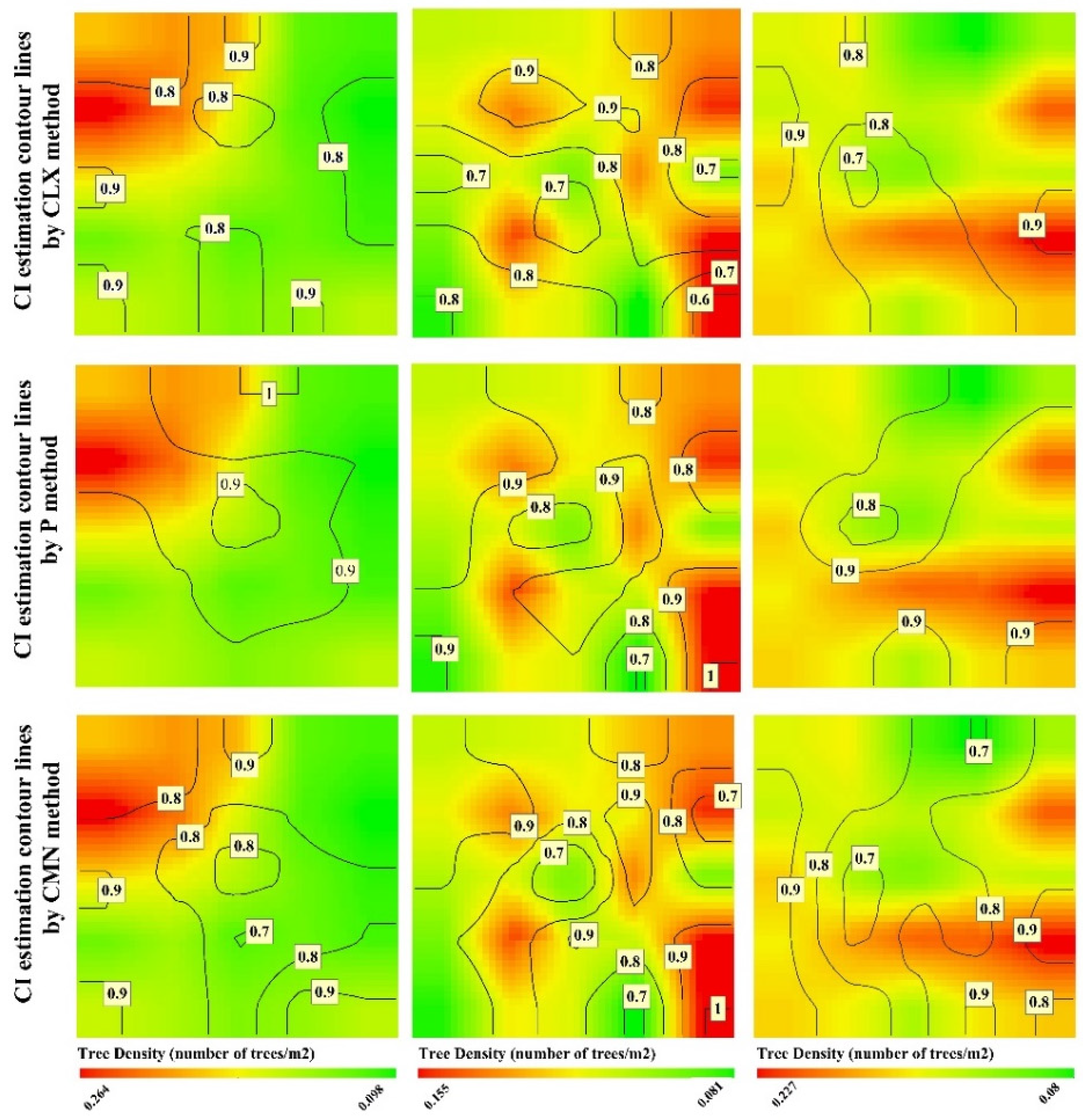
Boxplots were used to compare the differences in the results using the LX, CC, CLX, P, and CMN methods; kernel density analysis was used to represent the plant number densities of broad-leaved, coniferous, and mixed forests; and contour plots were used to represent the relationship between the stand density and the CI.

3. Results

3.1. Comparison of CI Estimation Results Using Various Methods

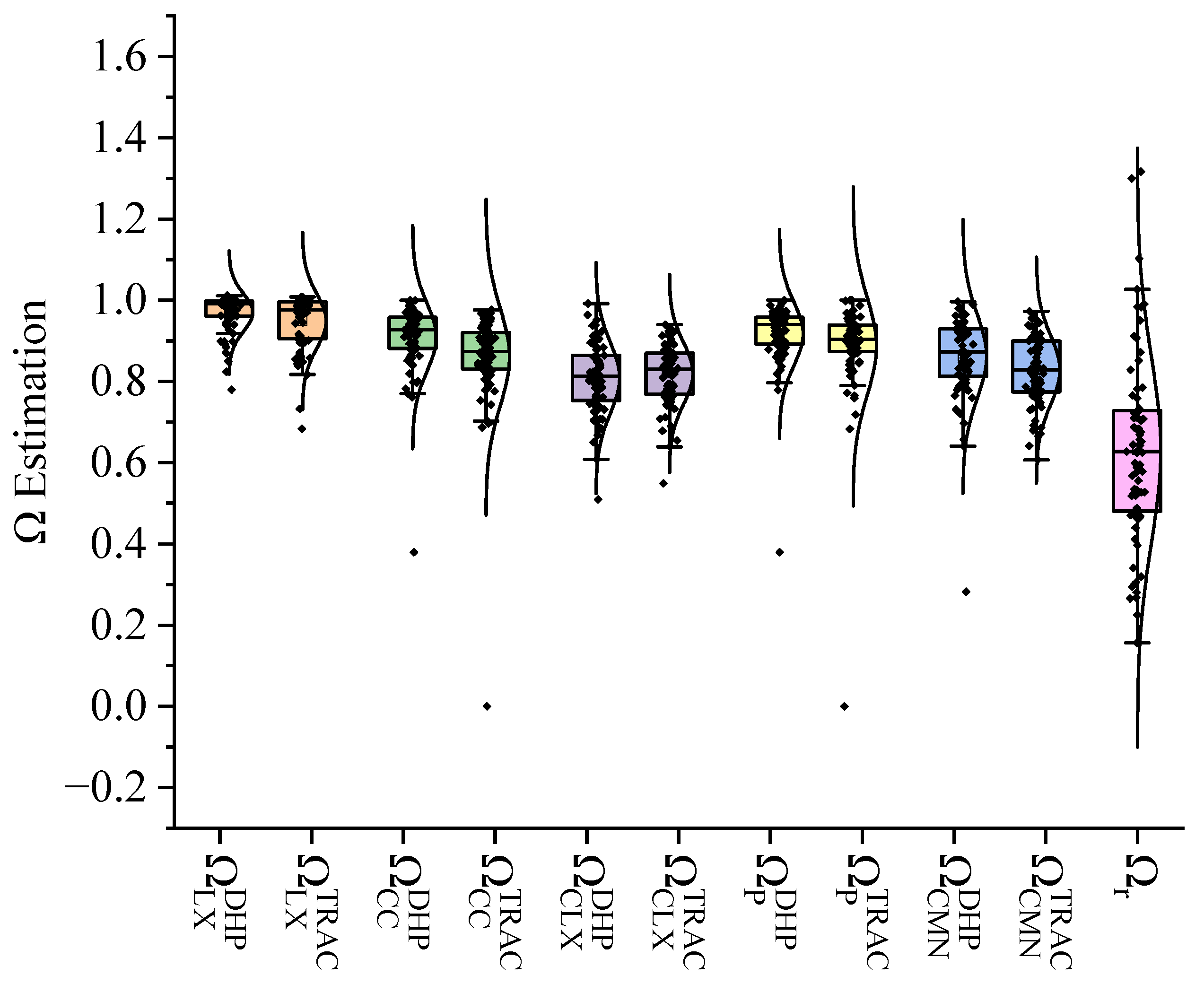
We set five transects, 100 m in length, to obtain the gap size distributions of foliage elements using the TRAC and DHP methods (Figure 3). The segment length was set to a width of 20 m with the suggestion of TRAC manuals and publications [64]. Then, the clumping index of the plot was estimated using the methods mentioned above. Moreover, the estimated CI was compared with the real clumping index (Ωr) using various methods in different forest types. These results show that the CI estimation results varied depending on the method selected (Figure 4). For DHP measurements, the relative errors of CI estimation using the ΩLX, ΩCC, ΩCLX, ΩP, and ΩCMN, and Ωr methods were 53.6%, 44%, 28.1%, 45.3%, and 36.4%, respectively. For TRAC measurements, the relative errors of CI estimation using the ΩLX, ΩCC, ΩCLX, ΩP, and ΩCMN, and Ωr methods were 50.2%, 36.2%, 29.8%, 40.4%, and 31.2%, respectively. CI estimation using the ΩCLX method exhibited the best accuracy among the five methods. The relative errors of CI estimation using the ΩCLX method were 28.1% and 29.8% for the DHP and TRAC measurements, respectively. Moreover, the accuracy values of CI estimation using the TRAC measurements were better than those of the DHP measurements, indicating that the TRAC measurements have better robustness for CI estimation.

3.2. Comparison of CI Estimation Results Using Various Methods

We compared the CI estimation results using various methods in different forest types. These results can be found in Figure 5. For broadleaf forests, CI estimation values using the ΩLX, ΩCC, ΩCLX, ΩP, and ΩCMN methods from TRAC measurements were 0.97 ± 0.04, 0.88 ± 0.05, 0.83 ± 0.06, 0.91 ± 0.05, and 0.82 ± 0.08, respectively. The CI estimation of the ΩLX, ΩCC, ΩCLX, ΩP, and ΩCMN methods exhibited an overestimating trend with relative errors of 59.6%, 45.7%, 37%, 51.1%, and 36.4%, respectively. CI estimation values using the ΩLX, ΩCC, ΩCLX, ΩP, and ΩCMN methods from DHP measurements were 0.98 ± 0.03, 0.93 ± 0.04, 0.89 ± 0.05, 0.94 ± 0.04, and 0.87 ± 0.06, respectively. The relative errors of CI estimation using the ΩLX, ΩCC, ΩCLX, ΩP, and ΩCMN methods from DHP measurements were 62.1%, 53.9%, 47.5%, 55.1%, and 44%, respectively.
For coniferous forests, CI estimation values using the ΩLX, ΩCC, ΩCLX, ΩP, and ΩCMN methods from TRAC measurements were 0.92 ± 0.09, 0.83 ± 0.19, 0.8 ± 0.1, 0.84 ± 0.19, and 0.83 ± 0.1, respectively. The relative errors of CI estimation using the ΩLX, ΩCC, ΩCLX, ΩP, and ΩCMN methods were 74.6%, 56.2%, 51.1%, 57.9%, and 56.8%, respectively. CI estimation values using the ΩLX, ΩCC, ΩCLX, ΩP, and ΩCMN methods from DHP measurements were 0.95 ± 0.06, 0.88 ± 0.12, 0.75 ± 0.08, 0.89 ± 0.12, and 0.85 ± 0.14, respectively. The relative errors of CI estimation using the ΩLX, ΩCC, ΩCLX, ΩP, and ΩCMN methods from DHP measurements were 80%, 66.9%, 41%, 67.3%, and 60.1%. At the same time, CI measurement values from TRAC and DHP were overestimated compared with the true values.
For mixed forests, CI estimation values using the ΩLX, ΩCC, ΩCLX, ΩP, and ΩCMN methods from TRAC measurements were 0.96 ± 0.06, 0.87 ± 0.06, 0.83 ± 0.06, 0.91 ± 0.05, and 0.83 ± 0.08, respectively. The relative errors of CI estimation using the ΩLX, ΩCC, ΩCLX, ΩP, and ΩCMN methods were 25.9%, 14.8%, 9.3%, 19.7%, and 9%, respectively. CI estimation values using the ΩLX, ΩCC, ΩCLX, ΩP, and ΩCMN methods from DHP measurements were 0.98 ± 0.04, 0.91 ± 0.07, 0.79 ± 0.05, 0.93 ± 0.05, and 0.86 ± 0.09, respectively. The relative errors of CI estimation using the ΩLX, ΩCC, ΩCLX, ΩP, and ΩCMN methods from DHP measurements were 28.4%, 20%, 3.6%, 22.1%, and 13.4%, respectively.
A comparison between the CI estimation results using both TRAC and DHP methods shows that there were no significant differences, even for the same CI estimation methods. For broadleaf forests, the relative errors of CI estimation using the ΩLX, ΩCC, ΩCLX, ΩP, and ΩCMN methods between different pieces of equipment were 1.5%, 5.4%, 7.2%, 2.6%, and 5.6%, respectively. Moreover, the differences in CI estimation for coniferous forests were 6.9%, 3%, 6.7%, 5.9%, and 5.5%, respectively. For mixed forests, these values changed to 4.5%, 2%, 5.2%, 2%, and 3.9%, respectively.

3.3. The Effect of the Segment Length on CI Estimation Using Different Methods

Optical methods were non-destructive and cheaper, but the CI estimation results were affected by the segment length on the transect [21]. Meanwhile, the segment size in the field measurements was usually arbitrarily decided, whereas the difference in the choices were derived from the difference in the CI estimation values [16]. Thus, we compared the CI estimation result with various segment lengths and discussed the influence of the segment length on CI estimation.
We estimated CI values with segment lengths of 1 m, 2 m, 4 m, 5 m, 10 m, 20 m, 50 m, and 100 m. CI estimation values using the ΩP method at various segment lengths were 0.97 ± 0.03, 0.97 ± 0.03, 0.96 ± 0.04, 0.93 ± 0.04, 0.99 ± 0.04, 0.92 ± 0.03, 0.93 ± 0.03, and 0.85 ± 0.03, respectively. CI estimation values using the ΩCC method at various segment lengths were 0.98 ± 0.04, 0.98 ± 0.04, 0.98 ± 0.03, 0.95 ± 0.04, 0.99 ± 0.02, 0.92 ± 0.06, 0.91 ± 0.03, and 0.84 ± 0.02, respectively. CI estimation values using the ΩLX method at various segment lengths were 0.73 ± 0.1, 0.69 ± 0.06, 0.73 ± 0.09, 0.79 ± 0.09, 0.90 ± 0.01, 0.88 ± 0.03, 0.93 ± 0.04, and 1.0 ± 0.01 respectively. CI estimation values using the ΩCLX method at various segment lengths were 0.72 ± 0.01, 0.62 ± 0.03, 0.79 ± 0.02, 0.72 ± 0.05, 0.92 ± 0.04, 0.81 ± 0.04, 0.85 ± 0.03, and 0.84 ± 0.03, respectively. CI estimation values using the ΩCMN method at various segment lengths were 0.97 ± 0.04, 0.98 ± 0.04, 0.97 ± 0.05, 0.84 ± 0.04, 1.0 ± 0.03, 0.91 ± 0.05, 0.89 ± 0.02, and 0.8 ± 0.04, respectively. The figure shows the estimated CI values with segment lengths of 1 m, 2 m, 4 m, 5 m, 10 m, 20 m, 50 m, and 100 m (Figure 6).
The results show that the CI estimations using the ΩLX and ΩCLX methods were more sensitive to the changes in the segment length compared with other methods. Furthermore, the ability to estimate the average CI was most stable when the segment length was between 10 and 50 m (the real CI Ωr = 0.532). CI estimation using the other three methods was less affected by the segment length compared to the results derived from the ΩLX and ΩCLX methods. This is because other methods do not rely on the random situation of the canopy within each segment. However, the CLX method can achieve the assumption of a random canopy in the segment by eliminating large light spots in the segment, indicating that the CLX method is less sensitive to the segment length compared to the LX method [17,19]. Compared with DHP measurements, there were similar results taken from the TRAC method. However, compared with DHP measurements, CI estimation values using the ΩCC, ΩP, and ΩCMN methods from the TRAC method were more stable. This was because the three methods had similar principles for CI estimation. Moreover, these methods were less affected by the segment length. Meanwhile, the estimated CI values using the ΩLX and ΩCLX methods were close to the real clumping index when the segment length was 2 m. However, the CI estimation values became closer and closer to the true value with an increase in the segment length. This is because the smaller the segment length, the more random the canopy distribution within the segment. However, if the segment length is too small, the possibility of a zero gap or a full gap in the segment increases, resulting in errors in the algorithm processing [48]. In addition, we found the smallest deviation with a segment length in the range of 10 m–50 m among different methods. The CI estimation values deviated the most when the segment length was 2 m. Furthermore, similar results can be found in different forest-type plots. Therefore, the segment length can affect CI estimation and the segment length should be determined by CI estimation methods.

3.4. The Effect of the Tree Density on CI Estimation

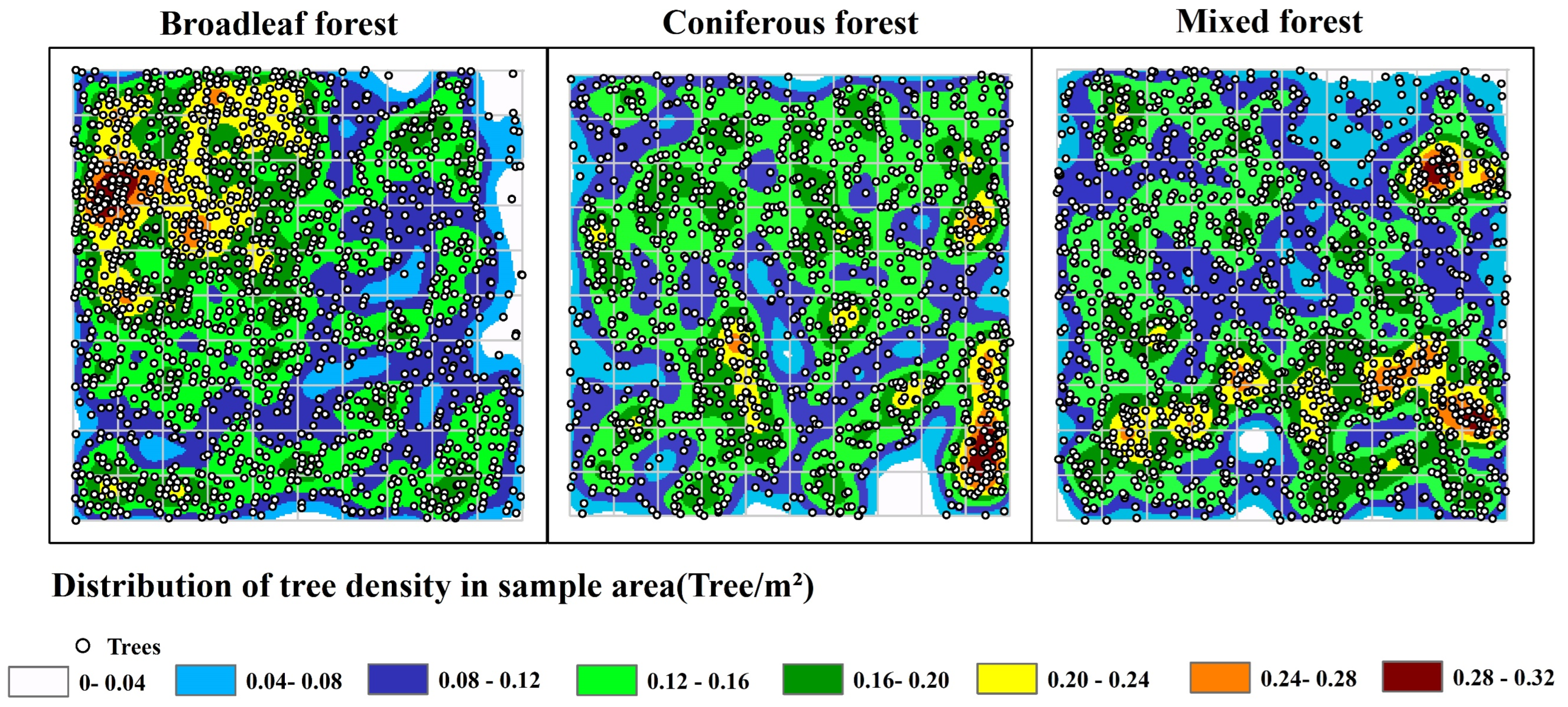
Various tree density values affect the transmission of direct sunlight in canopy environments and canopy gap distributions [19]. This may also have an impact on CI estimation using different methods. We calculated the tree density of plots in the broadleaf forest, the coniferous forest, and the mixed forest. Additionally, the tree density ranged from 0 to 0.08 (tree/m2), 0.08 to 0.16 (tree/m2), 0.16 to 0.24 (tree/m2), and 0.24 to 0.32 (tree/m2). The figure shows that the distribution of the trees had an obviously spatial heterogeneity effect in the different plots (Figure 7). This affects the sunlight transmitted to the canopy and leads to uncertainties in CI estimation when using optical equipment. Therefore, we compared the results of CI estimation among the scale plots in the different forest types.
We calculated the true clumping index using the litter trap, and then CI estimation was performed using the five methods mentioned above with TRAC measurements. Next, the contour lines of CI estimation using various methods were extracted with ARCGIS software. Finally, the results were overlapped in different tree density mapping studies, as shown in Figure 7. The results show that the real CI had an obviously spatial heterogeneity effect among the different plots too, and this feature was related to the spatial distribution of trees in the plot. The real CI increased when the tree density increased in the plots. This was because the distribution of the trees becomes random with an increase in the number of trees in one plot. In contrast, when the number of trees is smaller, the aggregated distribution becomes more obvious. According to the results shown in Figure 8, the CI estimation values varied with different methods. The relative error of CI estimation using the ΩLX method ranged from 41% to 67%. The relative error of CI estimation using the ΩCC method ranged from 31% to 62%. This value changed from 18% to 56% when the ΩCLX method was used. The relative error of CI estimation using the ΩP method ranged from 41% to 56%. This value changed from 18% to 60% when the ΩCMN method was used. In contrast, the accuracy of CI estimation using the ΩCLX method was better than that of other methods. The CI value estimated by the ΩCLX method was more similar to the real CI, followed by that of the ΩLX, ΩCC, ΩP, and ΩCMN methods. At the same time, the difference in the spatial distribution of the CI in plot scale was also obvious. Compared with the results used by other methods, the spatial distribution of CI estimation using the ΩCMN method was richer for describing the spatial heterogeneity of the CI. However, the accuracy of this method was not as good as the ΩCLX method.

4. Discussion

As a parameter used to describe the distribution of canopy foliage elements, the clumping index (CI) is a measurement of the clumping or random distribution of canopy environments in space, and it is very important to determine the radiation transfer of the canopy, the photosynthesis of the foliage, and the hydrological processes. At the moment, there are many methods used to obtain the CI, such as commercial optical instruments or satellite data [18]. The DHP, LAI-2200, and TRAC methods have frequently been used to estimate the CI during field measurements [16,17,21]. However, CI estimation varies depending on the estimation method and the accuracy of the different methods is still unverified. Meanwhile, the choice of a specific method varies depending on the vegetation type and field conditions [12]. Therefore, we compared the CI estimation values with the CI value (calculated by the litter collection method) using the LX, CC, CLX, P, and CMN methods. The advantages and disadvantages of different methods were compared and the influence factors were analyzed.

4.1. Differences in CI Estimation Methods

In this study, the accuracy values of CI estimation using the LX, CC, CLX, P, and CMN methods were compared. The results show different CI estimation methods lead to huge differences in the estimation results. Zou et al. conducted a comparative study of CI estimation on three algorithms, namely, the gap size distribution method, the finite-length average method, and the segregation coefficient method [17]. The results showed that there were great differences among the three algorithms, and that the gap size distribution method and the segregation coefficient method were the most stable. However, the results of the segregation coefficient method were seriously low compared with the other two methods. Similar results can also be found in this study. We compared the accuracy of CI estimation using the LX, CC, CLX, P, and CMN methods. The results indicate that CI estimation using the ΩCLX method exhibited better results compared to the other methods. Similar results can also be found in previous research [21,22,23]. Chen mentioned that the CI calculated by the CC method was different from that of the P method [22,23]. Chu et al. compared the CI estimation values using the finite-length average method, the gap size distribution method, and the path length distribution method. The results indicate an overestimating trend for the LX method in the low clumping area or during the low clumping growth period. This was because this method can fail when there is no gap in the finite length. Instead, in the high clumping area or during the high clumping growth period, the gap size distribution method will underestimate the clumping effect [58].
In addition, we found that the accuracy values of CI estimation using TRAC measurements were different from those for DHP measurements. This was because the DHP method offered a directional sampling of canopy gaps and because the accuracy of CI estimation from the DHP method was dependent on the subjective classification procedure of plant pixels and gaps [8]. However, the TRAC method calculated the canopy gap size distribution using transmitted sunlight recordings along a transect. These results are influenced by a solar zenith angle, a limited field-of-view light beam, a gap threshold, and a gap removal procedure [16,22,23].

4.2. Effecting Factors of the CI Estimation Method

Indirect optical methods for CI estimation were non-destructive and cost-effective, but these common instruments such as DHP, LAI-2200, and TRAC were subject to the influence of segment selection. In this study, we estimated the CI with segment lengths of 1 m, 2 m, 4 m, 5 m, 10 m, 20 m, 50 m, and 100 m, and compared the CI estimation results with various segment lengths. The results indicate that the ΩLX and ΩCLX methods were more sensitive to the changes in the segment length compared with other methods. This result was similar to previous research findings. Pisek et al. concluded that both the LX and CLX methods were highly sensitive to segment length compared to the actual measurements of DHP and TRAC, and the CI estimation error when using the DHP and TRAC methods decreased with a decrease in the segment length [19]. Woodgate found that the LX method was more sensitive to segment length than the CC or CLX methods, among others [49]. In addition, we found that the accuracy of CI estimation decreased with a decrease in the segment length. Gonsamo et al. measured the canopy gap with DHP and CI estimation using the LX method. The results indicate that the CI estimation values decreased with a decrease in the segment size from 15° to 2.5° [65]. This was because the random assumption for low plants was not true and because it was not feasible to measure the small segment size with the high probability of obtaining a zero-gap fraction. To solve the problem, some scholars proposed to add sky pixels into the fragment [25,66]. Gonsamo et al. improved the LX method by merging the gap-free part with the adjacent gap-filled part, but this improvement affected the choice of optimal segment length and thus impacted CI estimation [65].
The various tree densities affect the transmission of direct sunlight and gap distributions in canopy environments [19]. Therefore, this may have an impact on CI estimation when different methods are used. In this study, we calculated CI estimation values using different methods and compared the results among various tree densities in the broadleaf forest, the coniferous forest, and the mixed forest. The results indicate that the clumping index had significant spatial heterogeneity. The estimation results in different forest types also varied. Some research results have indicated that different stand types have different CI estimation values when different methods are used [17,19,67]. Craig Macfarlane et al. found that the CLX method had significant advantages over the CC method in a jarrah forest in Australia [68]. Woodgate found that the CLX method provided better CI estimation values than the CC and LX methods in eucalyptus forests [49]. Pisek et al. found that the CLX method performed better compared to the CC, LX, and CMN methods in Scots pine forests [19]. Similar results can also be found in this study. In general, the CLX method is better than the other methods used in this study. This is because the CLX method can not only eliminate the problem of the non-randomness in the canopy inside the segment, but can also normalize the whole line, resulting in more obvious random effects at the transect level [19]. In addition, the ΩCMN method can effectively describe the spatial distribution of the CI. Moreover, it can reflect the change characteristics of the clumping index with various tree densities. Therefore, in field measurements, the CI estimation method should be decided after considering the light conditions, the solar zenith, the segment length or size, and the stand types [69,70].

5. Conclusions

In this study, we set three 100 × 100 m plots of different forest types and estimated the clumping index using the measurements from TRAC, LAI-2200, DHP, and litter collection methods. Then, the results of CI estimation at various segment lengths using the LX, CC, CLX, P, and CMN methods were compared. The results indicate the following:
(1)
The segment length has a significant effect on CI estimation with various methods. The CI estimation accuracy values of the LX and CLX methods increase with a decrease in segment lengths. The CI estimation results using the CC, P, LX, and CLX methods are the most similar under the segment lengths in the range of 10 m to 50 m. Moreover, CI estimation using the CLX method is most effective at a segment length of 2 m.
(2)
The CI has an obviously spatial heterogeneity effect in the different plots. Compared with the true CI, there is significant difference in CI estimation when using various methods. Moreover, the spatial distribution of the CI, estimated using the ΩCMN method, is more useful when describing the spatial heterogeneity patterns of the CI.

Author Contributions

Y.Y. and X.Y. conceived and designed the experiments; Z.L. performed the experiments and analyzed the data; X.Y. and Z.L. wrote the paper; X.Y., Y.Y. and W.F. reviewed and edited the paper. All authors have read and agreed to the published version of the manuscript.

Funding

This research was funded by the National Natural Science Foundation of China (grant numbers 31870621 and 31971580); the Fundamental Research Funds for the Central Universities of China (grant numbers 2572021BA08, 2572019BA10, and 2572019CP12); and the China Postdoctoral Science Foundation (grant number 2019M661239).

Data Availability Statement

Not application.

Conflicts of Interest

The authors declare no conflict of interest.

References

  1. Peng, J.; Fan, W.; Wang, L.; Xu, X.; Li, J.; Zhang, B.; Tian, D. Modeling the Directional Clumping Index of Crop and Forest. Remote Sens. 2018, 10, 1576. [Google Scholar] [CrossRef] [Green Version]
  2. Duthoit, S.; Demarez, V.; Gastellu-Etchegorry, J.-P.; Martin, E.; Roujean, J.-L. Assessing the effects of the clumping phenomenon on BRDF of a maize crop based on 3D numerical scenes using DART model. Agric. For. Meteorol. 2008, 148, 1341–1352. [Google Scholar] [CrossRef] [Green Version]
  3. Qi, J.; Xie, D.; Jiang, J.; Huang, H. 3D radiative transfer modeling of structurally complex forest canopies through a lightweight boundary-based description of leaf clusters. Remote Sens. Environ. 2022, 283, 113301. [Google Scholar] [CrossRef]
  4. Nilson, T. Inversion of gap frequency data in forest stands. Agric. For. Meteorol. 1999, 98, 437–448. [Google Scholar] [CrossRef]
  5. Fassnacht, K.S.; Gower, S.T.; Norman, J.M.; McMurtric, R.E. A comparison of optical and direct methods for estimating foliage surface area index in forests. Agric. For. Meteorol. 1994, 71, 183–207. [Google Scholar] [CrossRef]
  6. Jonckheere, I.; Fleck, S.; Nackaerts, K.; Muys, B.; Coppin, P.; Weiss, M.; Baret, F. Review of methods for in situ leaf area index determination: Part I. Theories, sensors and hemispherical photography. Agric. For. Meteorol. 2004, 121, 19–35. [Google Scholar] [CrossRef]
  7. Ma, L.; Zheng, G.; Wang, X.; Li, S.; Lin, Y.; Ju, W. Retrieving forest canopy clumping index using terrestrial laser scanning data. Remote Sens. Environ. 2018, 210, 452–472. [Google Scholar] [CrossRef] [Green Version]
  8. Chen, J.M.; Black, T. Defining leaf area index for non-flat leaves. Plant Cell Environ. 1992, 15, 421–429. [Google Scholar] [CrossRef]
  9. Nilson, T. A theoretical analysis of the frequency of gaps in plant stands. Agric. Meteorol. 1971, 8, 25–38. [Google Scholar] [CrossRef]
  10. Hilty, J.; Muller, B.; Pantin, F.; Leuzinger, S. Plant growth: The What, the How, and the Why. New Phytol. 2021, 232, 25–41. [Google Scholar] [CrossRef]
  11. Fang, H.; Baret, F.; Plummer, S.; Schaepman-Strub, G. An Overview of Global Leaf Area Index (LAI): Methods, Products, Validation, and Applications. Rev. Geophys. 2019, 57, 739–799. [Google Scholar] [CrossRef]
  12. Fang, H.; Liu, W.; Li, W.; Wei, S. Estimation of the directional and whole apparent clumping index (ACI) from indirect optical measurements. ISPRS J. Photogramm. Remote Sens. 2018, 144, 1–13. [Google Scholar] [CrossRef]
  13. Yang, K.; Ryu, Y.; Dechant, B.; Berry, J.A.; Hwang, Y.; Jiang, C.; Kang, M.; Kim, J.; Kimm, H.; Kornfeld, A. Sun-induced chlorophyll fluorescence is more strongly related to absorbed light than to photosynthesis at half-hourly resolution in a rice paddy. Remote Sens. Environ. 2018, 216, 658–673. [Google Scholar] [CrossRef]
  14. Béland, M.; Baldocchi, D. Is foliage clumping an outcome of resource limitations within forests? Agric. For. Meteorol. 2020, 295, 108185. [Google Scholar] [CrossRef]
  15. Woodgate, W.; Disney, M.; Armston, J.D.; Jones, S.D.; Suarez, L.; Hill, M.J.; Wilkes, P.; Soto-Berelov, M.; Haywood, A.; Mellor, A. An improved theoretical model of canopy gap probability for Leaf Area Index estimation in woody ecosystems. For. Ecol. Manag. 2015, 358, 303–320. [Google Scholar] [CrossRef]
  16. Fang, H. Canopy clumping index (CI): A review of methods, characteristics, and applications. Agric. For. Meteorol. 2021, 303, 108374. [Google Scholar] [CrossRef]
  17. Zou, J.; Zhuang, Y.; Chianucci, F.; Mai, C.; Lin, W.; Leng, P.; Luo, S.; Yan, B. Comparison of Seven Inversion Models for Estimating Plant and Woody Area Indices of Leaf-on and Leaf-off Forest Canopy Using Explicit 3D Forest Scenes. Remote Sens. 2018, 10, 1297. [Google Scholar] [CrossRef] [Green Version]
  18. Lang, A.; Yueqin, X. Estimation of leaf area index from transmission of direct sunlight in discontinuous canopies. Agric. For. Meteorol. 1986, 37, 229–243. [Google Scholar] [CrossRef]
  19. Pisek, J.; Lang, M.; Nilson, T.; Korhonen, L.; Karu, H. Comparison of methods for measuring gap size distribution and canopy nonrandomness at Järvselja RAMI (RAdiation transfer Model Intercomparison) test sites. Agric. For. Meteorol. 2011, 151, 365–377. [Google Scholar] [CrossRef]
  20. Demarez, V.; Duthoit, S.; Baret, F.; Weiss, M.; Dedieu, G. Estimation of leaf area and clumping indexes of crops with hemispherical photographs. Agric. For. Meteorol. 2008, 148, 644–655. [Google Scholar] [CrossRef]
  21. Leblanc, S.G. Correction to the plant canopy gap-size analysis theory used by the Tracing Radiation and Architecture of Canopies instrument. Appl. Opt. 2002, 41, 7667–7670. [Google Scholar] [CrossRef]
  22. Chen, J.M.; Cihlar, J. Quantifying the effect of canopy architecture on optical measurements of leaf area index using two gap size analysis methods. IEEE Trans. Geosci. Remote Sens. 1995, 33, 777–787. [Google Scholar] [CrossRef]
  23. Chen, J.M.; Cihlar, J. Plant canopy gap-size analysis theory for improving optical measurements of leaf-area index. Appl. Opt. 1995, 34, 6211–6222. [Google Scholar] [CrossRef] [Green Version]
  24. Ryu, Y.; Sonnentag, O.; Nilson, T.; Vargas, R.; Kobayashi, H.; Wenk, R.; Baldocchi, D.D. How to quantify tree leaf area index in an open savanna ecosystem: A multi-instrument and multi-model approach. Agric. For. Meteorol. 2010, 150, 63–76. [Google Scholar] [CrossRef]
  25. Leblanc, S.G.; Chen, J.M.; Fernandes, R.; Deering, D.W.; Conley, A. Methodology comparison for canopy structure parameters extraction from digital hemispherical photography in boreal forests. Agric. For. Meteorol. 2005, 129, 187–207. [Google Scholar] [CrossRef] [Green Version]
  26. Leblanc, S.; Fournier, R. Hemispherical photography simulations with an architectural model to assess retrieval of leaf area index. Agric. For. Meteorol. 2014, 194, 64–76. [Google Scholar] [CrossRef]
  27. Chen, J.M. Optically-based methods for measuring seasonal variation of leaf area index in boreal conifer stands. Agric. For. Meteorol. 1996, 80, 135–163. [Google Scholar] [CrossRef]
  28. Bréda, N.J. Ground-based measurements of leaf area index: A review of methods, instruments and current controversies. J. Exp. Bot. 2003, 54, 2403–2417. [Google Scholar] [CrossRef] [Green Version]
  29. Jurik, T.W.; Briggs, G.M.; Gates, D.M. A comparison of four methods for determining leaf area index in successional hardwood forests. Can. J. For. Res. 1985, 15, 1154–1158. [Google Scholar] [CrossRef]
  30. Liu, Z.; Chen, J.M.; Jin, G.; Qi, Y. Estimating seasonal variations of leaf area index using litterfall collection and optical methods in four mixed evergreen–deciduous forests. Agric. For. Meteorol. 2015, 209, 36–48. [Google Scholar] [CrossRef]
  31. Le Dantec, V.; Dufrêne, E.; Saugier, B. Interannual and spatial variation in maximum leaf area index of temperate deciduous stands. For. Ecol. Manag. 2000, 134, 71–81. [Google Scholar] [CrossRef]
  32. Mencuccini, M.; Grace, J. Climate influences the leaf area/sapwood area ratio in Scots pine. Tree Physiol. 1995, 15, 1–10. [Google Scholar] [CrossRef] [PubMed] [Green Version]
  33. Smith, N. Predicting radiation attenuation in stands of Douglas-fir. For. Sci. 1991, 37, 1213–1223. [Google Scholar]
  34. Marshall, J.; Waring, R. Comparison of methods of estimating leaf-area index in old-growth Douglas-fir. Ecology 1986, 67, 975–979. [Google Scholar] [CrossRef] [Green Version]
  35. Liu, Z.; Jin, G.; Chen, J.M.; Qi, Y. Evaluating optical measurements of leaf area index against litter collection in a mixed broadleaved-Korean pine forest in China. Trees 2015, 29, 59–73. [Google Scholar] [CrossRef]
  36. Guindin-Garcia, N.; Gitelson, A.A.; Arkebauer, T.J.; Shanahan, J.; Weiss, A. An evaluation of MODIS 8-and 16-day composite products for monitoring maize green leaf area index. Agric. For. Meteorol. 2012, 161, 15–25. [Google Scholar] [CrossRef] [Green Version]
  37. Myneni, R.B.; Ramakrishna, R.; Nemani, R.; Running, S.W. Estimation of global leaf area index and absorbed PAR using radiative transfer models. IEEE Trans. Geosci. Remote Sens. 1997, 35, 1380–1393. [Google Scholar] [CrossRef] [Green Version]
  38. Curran, P. Multispectral remote sensing for the estimation of green leaf area index. Philos. Trans. R. Soc. Lond. Ser. A Math. Phys. Sci. 1983, 309, 257–270. [Google Scholar]
  39. Chen, J.M.; Rich, P.M.; Gower, S.T.; Norman, J.M.; Plummer, S. Leaf area index of boreal forests: Theory, techniques, and measurements. J. Geophys. Res. Atmos. 1997, 102, 29429–29443. [Google Scholar] [CrossRef] [Green Version]
  40. He, L.; Chen, J.M.; Pisek, J.; Schaaf, C.B.; Strahler, A.H. Global clumping index map derived from the MODIS BRDF product. Remote Sens. Environ. 2012, 119, 118–130. [Google Scholar] [CrossRef]
  41. Gonsamo, A.; Chen, J.M. Improved LAI algorithm implementation to MODIS data by incorporating background, topography, and foliage clumping information. IEEE Trans. Geosci. Remote Sens. 2013, 52, 1076–1088. [Google Scholar] [CrossRef]
  42. Chen, J.M.; Mo, G.; Pisek, J.; Liu, J.; Deng, F.; Ishizawa, M.; Chan, D. Effects of foliage clumping on the estimation of global terrestrial gross primary productivity. Glob. Biogeochem. Cycles 2012, 26, GB1019. [Google Scholar] [CrossRef]
  43. Dong, Y.; Jiao, Z.; Yin, S.; Zhang, H.; Zhang, X.; Cui, L.; He, D.; Ding, A.; Chang, Y.; Yang, S. Influence of snow on the magnitude and seasonal variation of the clumping index retrieved from MODIS BRDF products. Remote Sens. 2018, 10, 1194. [Google Scholar] [CrossRef] [Green Version]
  44. Chen, J.; Menges, C.; Leblanc, S. Global mapping of foliage clumping index using multi-angular satellite data. Remote Sens. Environ. 2005, 97, 447–457. [Google Scholar] [CrossRef]
  45. Li, Y.; Fang, H. Real-Time Software for the Efficient Generation of the Clumping Index and Its Application Based on the Google Earth Engine. Remote Sens. 2022, 14, 3837. [Google Scholar] [CrossRef]
  46. Bao, Y.; Ni, W.; Wang, D.; Yue, C.; He, H.; Verbeeck, H. Effects of tree trunks on estimation of clumping index and LAI from HemiView and Terrestrial LiDAR. Forests 2018, 9, 144. [Google Scholar] [CrossRef] [Green Version]
  47. Li, Y.; Guo, Q.; Su, Y.; Tao, S.; Zhao, K.; Xu, G. Retrieving the gap fraction, element clumping index, and leaf area index of individual trees using single-scan data from a terrestrial laser scanner. ISPRS J. Photogramm. Remote Sens. 2017, 130, 308–316. [Google Scholar] [CrossRef]
  48. Woodgate, W. In-Situ Leaf Area Index Estimate Uncertainty in Forests: Supporting Earth Observation Product Calibration and Validation; RMIT University Melbourne: Melbourne, VIC, Australia, 2015. [Google Scholar]
  49. Woodgate, W.; Armston, J.D.; Disney, M.; Jones, S.D.; Suarez, L.; Hill, M.J.; Wilkes, P.; Soto-Berelov, M. Quantifying the impact of woody material on leaf area index estimation from hemispherical photography using 3D canopy simulations. Agric. For. Meteorol. 2016, 226, 1–12. [Google Scholar] [CrossRef]
  50. Yin, S.; Jiao, Z.; Dong, Y.; Zhang, X.; Cui, L.; Xie, R.; Guo, J.; Li, S.; Zhu, Z.; Tong, Y. Evaluation of the Consistency of the Vegetation Clumping Index Retrieved from Updated MODIS BRDF Data. Remote Sens. 2022, 14, 3997. [Google Scholar] [CrossRef]
  51. Zhao, Y.; Ma, Y.; Quackenbush, L.J.; Zhen, Z. Estimation of Individual Tree Biomass in Natural Secondary Forests Based on ALS Data and WorldView-3 Imagery. Remote Sens. 2022, 14, 271. [Google Scholar] [CrossRef]
  52. Masinda, M.M.; Li, F.; Liu, Q.; Sun, L.; Hu, T. Prediction model of moisture content of dead fine fuel in forest plantations on Maoer Mountain, Northeast China. J. For. Res. 2021, 32, 2023–2035. [Google Scholar] [CrossRef]
  53. Wang, C. Biomass allometric equations for 10 co-occurring tree species in Chinese temperate forests. For. Ecol. Manag. 2006, 222, 9–16. [Google Scholar] [CrossRef]
  54. Chen, J.M.; Cihlar, J. Retrieving leaf area index of boreal conifer forests using Landsat TM images. Remote Sens. Environ. 1996, 55, 153–162. [Google Scholar] [CrossRef]
  55. Eriksson, H.; Eklundh, L.; Hall, K.; Lindroth, A. Estimating LAI in deciduous forest stands. Agric. For. Meteorol. 2005, 129, 27–37. [Google Scholar] [CrossRef]
  56. Baret, F.; de Solan, B.; Lopez-Lozano, R.; Ma, K.; Weiss, M. GAI estimates of row crops from downward looking digital photos taken perpendicular to rows at 57.5° zenith angle: Theoretical considerations based on 3D architecture models and application to wheat crops. Agric. For. Meteorol. 2010, 150, 1393–1401. [Google Scholar] [CrossRef]
  57. Nomura, K.; Saito, M.; Kitayama, M.; Goto, Y.; Nagao, K.; Yamasaki, H.; Iwao, T.; Yamazaki, T.; Tada, I.; Kitano, M. Leaf area index estimation of a row-planted eggplant canopy using wide-angle time-lapse photography divided according to view-zenith-angle contours. Agric. For. Meteorol. 2022, 319, 108930. [Google Scholar] [CrossRef]
  58. Wei, S.; Fang, H. Estimation of canopy clumping index from MISR and MODIS sensors using the normalized difference hotspot and darkspot (NDHD) method: The influence of BRDF models and solar zenith angle. Remote Sens. Environ. 2016, 187, 476–491. [Google Scholar] [CrossRef]
  59. Whitford, K.; Colquhoun, I.; Lang, A.; Harper, B. Measuring leaf area index in a sparse eucalypt forest: A comparison of estimates from direct measurement, hemispherical photography, sunlight transmittance and allometric regression. Agric. For. Meteorol. 1995, 74, 237–249. [Google Scholar] [CrossRef]
  60. Chen, J.; Black, T. Foliage area and architecture of plant canopies from sunfleck size distributions. Agric. For. Meteorol. 1992, 60, 249–266. [Google Scholar] [CrossRef]
  61. Miller, E.E.; Norman, J.M. A Sunfleck Theory for Plant Canopies I. Lengths of Sunlit Segments along a Transect 1. Agron. J. 1971, 63, 735–738. [Google Scholar] [CrossRef]
  62. Hu, R.; Yan, G.; Mu, X.; Luo, J. Indirect measurement of leaf area index on the basis of path length distribution. Remote Sens. Environ. 2014, 155, 239–247. [Google Scholar] [CrossRef]
  63. Yan, G.; Hu, R.; Luo, J.; Weiss, M.; Jiang, H.; Mu, X.; Xie, D.; Zhang, W. Review of indirect optical measurements of leaf area index: Recent advances, challenges, and perspectives. Agric. For. Meteorol. 2019, 265, 390–411. [Google Scholar] [CrossRef]
  64. Kuusk, A.; Pisek, J.; Lang, M.; Märdla, S. Estimation of Gap Fraction and Foliage Clumping in Forest Canopies. Remote Sens. 2018, 10, 1153. [Google Scholar] [CrossRef] [Green Version]
  65. Gonsamo, A.; Walter, J.-M.N.; Pellikka, P. Sampling gap fraction and size for estimating leaf area and clumping indices from hemispherical photographs. Can. J. For. Res. 2010, 40, 1588–1603. [Google Scholar] [CrossRef]
  66. Van Gardingen, P.; Jackson, G.; Hernandez-Daumas, S.; Russell, G.; Sharp, L. Leaf area index estimates obtained for clumped canopies using hemispherical photography. Agric. For. Meteorol. 1999, 94, 243–257. [Google Scholar] [CrossRef]
  67. Kucharik, C.J.; Norman, J.M.; Gower, S.T. Characterization of radiation regimes in nonrandom forest canopies: Theory, measurements, and a simplified modeling approach. Tree Physiol. 1999, 19, 695–706. [Google Scholar] [CrossRef] [Green Version]
  68. Macfarlane, C.; Hoffman, M.; Eamus, D.; Kerp, N.; Higginson, S.; McMurtrie, R.; Adams, M. Estimation of leaf area index in eucalypt forest using digital photography. Agric. For. Meteorol. 2007, 143, 176–188. [Google Scholar] [CrossRef]
  69. Leblanc, S.G.; Chen, J.M. A practical scheme for correcting multiple scattering effects on optical LAI measurements. Agric. For. Meteorol. 2001, 110, 125–139. [Google Scholar] [CrossRef]
  70. Zou, J.; Yan, G.; Chen, L. Estimation of canopy and woody components clumping indices at three mature picea crassifolia forest stands. IEEE J. Sel. Top. Appl. Earth Obs. Remote Sens. 2015, 8, 1413–1422. [Google Scholar] [CrossRef]
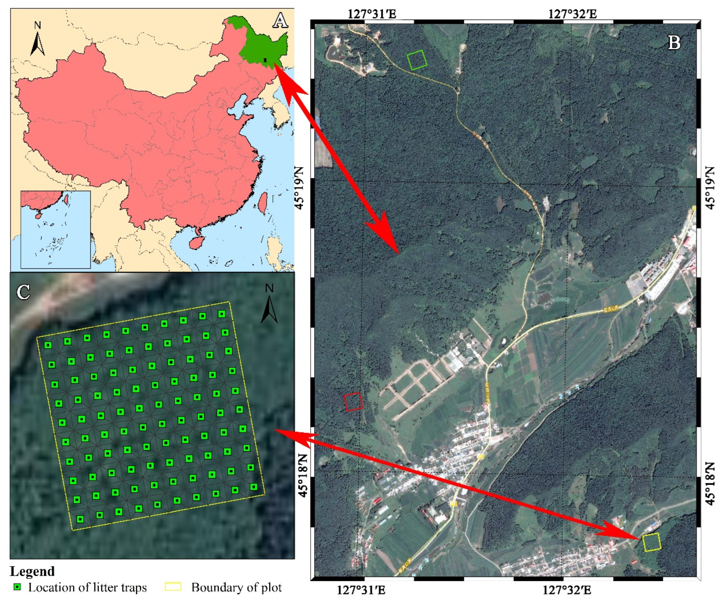
Figure 1. Study area map and LAI-2200 measurement points, TRAC transects, and leaf litter collection measurement points. ((A) was the overview of the research regeion; (B) was the overview of the plots; (C) was the positions of the measurements. Note: in (B), the yellow rectangle is the broadleaf forest, the red rectangle is the coniferous forest, and the green rectangle is the mixed forest).
Remotesensing 15 00471 g001
Figure 2. Photos of the field measurement process.
Remotesensing 15 00471 g002
Figure 3. Spatial distribution of measuring points of LAI-2200 and DHP and the TRAC transect line.
Remotesensing 15 00471 g003
Figure 4. Comparison of CI estimation values using different methods. (Note: the black curve on the right indicates that the data are normally distributed.)
Remotesensing 15 00471 g004
Figure 5. A comparison of CI estimation values using various methods in different forest types. (Note: the black curve on the right indicates that the data are normally distributed.).
Remotesensing 15 00471 g005
Figure 6. A comparison of CI estimation values with various segment lengths using the ΩLX, ΩCC, ΩCLX, ΩP, and ΩCMN methods.
Remotesensing 15 00471 g006
Figure 7. Distribution of the trees and their density in the plots.
Remotesensing 15 00471 g007
Figure 8. The spatial distribution of CI estimation using different methods in the plot (note: the contour lines show the CI estimation using various methods).
Remotesensing 15 00471 g008aRemotesensing 15 00471 g008b
Table 1. Basic tree information table of the three plots.
Sample TypeMajor SpeciesNumber of Trees (Number)Mean DBH (cm)Relative Dominance (%)SLA (cm2 × g−1)
Broad-leaved forestJuglans mandshurica Maxim.150811.87100213.62
Coniferous forestPinus sylvestris Linn.49626.8468.1967
Pinus koraiensis Sieb.19215.9114.3778.91
Fraxinus mandschurica Rupr.3821.265.08305.96
Ulmus pumila L. 20041.998.94245.48
Others21311.853.41——
Total113926.6100——
Mixed forestBetula platyphylla Suk.35727.8439.85195.46
Fraxinus mandschurica Rupr.24433.4116.61305.96
Pinus koraiensis Sieb.25631.755.7478.91
Quercus mongolica Fisch.9851.210.84253.94
Larix gmelini Rupr.11244.0711.66159.22
Ulmus pumila L. 23334.558.19245.48
Others8714.57.11——
Total1387237.31100——
Disclaimer/Publisher’s Note: The statements, opinions and data contained in all publications are solely those of the individual author(s) and contributor(s) and not of MDPI and/or the editor(s). MDPI and/or the editor(s) disclaim responsibility for any injury to people or property resulting from any ideas, methods, instructions or products referred to in the content.