Article

A Multiscale Spatiotemporal Fusion Network Based on an Attention Mechanism

1
College of Computer, Chongqing University of Posts and Telecommunications, Chongqing 400065, China
2
Chongqing Key Laboratory of Image Cognition, Chongqing University of Posts and Telecommunications, Chongqing 400065, China
3
School of Cyber Security and Information Law, Chongqing University of Posts and Telecommunications, Chongqing 400065, China
*
Author to whom correspondence should be addressed.
These authors contributed equally to this work.
Remote Sens. 2023, 15(1), 182; https://doi.org/10.3390/rs15010182
Submission received: 7 November 2022 / Revised: 21 December 2022 / Accepted: 23 December 2022 / Published: 29 December 2022
(This article belongs to the Section Remote Sensing Image Processing)

Abstract

:
Spatiotemporal fusion is an effective and cost-effective method to obtain both high temporal resolution and high spatial resolution images. However, existing methods do not sufficiently extract the deeper features of the image, resulting in fused images which do not recover good topographic detail and poor fusion quality. In order to obtain higher quality spatiotemporal fusion images, a novel spatiotemporal fusion method based on deep learning is proposed in this paper. The method combines an attention mechanism and a multiscale feature fusion network to design a network that more scientifically explores deeper features of the image for different input image characteristics. Specifically, a multiscale feature fusion module is introduced into the spatiotemporal fusion task and combined with an efficient spatial-channel attention module to improve the capture of spatial and channel information while obtaining more effective information. In addition, we design a new edge loss function and incorporate it into the compound loss function, which helps to generate fused images with richer edge information. In terms of both index performance and image details, our proposed model has excellent results on both datasets compared with the current mainstream spatiotemporal fusion methods.

Graphical Abstract

1. Introduction

The study and utilization of remote-sensing images is becoming more and more meaningful [1], it has become a critical and urgent task to obtain remote-sensing satellite images with both high spatial resolution and high temporal resolution. Although the progress of sensor technology has generated great convenience for the study of remote-sensing images [2], individual satellites are still unable to obtain high spatial resolution images with dense time series, and cost and technical bottlenecks are the main reasons for this problem [3,4].
Spatiotemporal fusion is a data post-processing technology developed to reduce the limitation of hardware technology. The fusion process generally requires two data sources [5], one of which has high spatial resolution and low temporal resolution (hereinafter referred to as fine resolution images), such as the Landsat-8 satellite, which can obtain spatial resolution images of 30 m with a repetition period of 16 days [6]. Another data source has high temporal resolution and low spatial resolution (hereinafter referred to as rough resolution images). These include the moderate resolution imaging spectrometer (MODIS), which can obtain daily observation data of the Earth, but most of their spatial resolution is not high, at only 500 m or so [7]. MODIS sensors are capable of acquiring images with low spatial resolution in intensive time (hereinafter referred to as coarse resolution images). The spatiotemporal fusion method can combine the daily data acquired by MODIS sensors and the fine resolution images acquired by Landsat satellites to generate high-spatial-resolution-fused image data with dense time series.
In general, there are four models of spatiotemporal fusion: (1) transformation-based; (2) pixel-reconstruction-based; (3) Bayesian-based; and (4) learning-based models [8,9]. Based on the data transformation model, original image pixels are mapped to an abstract space to perform fusion and obtain high-resolution data at unknown times [10]. The basic idea of the pixel reconstruction-based model is to select pixels near the target pixel to participate in the reconstruction of the target pixel, in which a series of specific rules need to be set. Typical examples include the spatial and temporal adaptive reflectance fusion model (STARFM) [11] and the spatial and temporal adaptive algorithm for mapping reflectance changes (STAARCH) [12]. Bayesian-based models [13] use the Bayesian statistical principle in mathematical statistics, such as the unified fusion method [14] and Bayesian maximum entropy method [15]. Bayesian-based models have advantages in processing different input images to produce better prediction results [5]. However, most of the above traditional algorithms rely on conditions set in advance and are relatively influenced by the quality of the dataset, and their performance is mostly unstable.
Learning-based models have been gradually accepted and have become a new research hotspot. These models are expected to obtain better fusion results than traditional fusion models, especially in the prediction of land cover change. A learning-based fusion model basically does not need to design fusion rules manually. It can automatically learn the best basic features from various quality input datasets and generate high-quality fused images. At present, there are two main ways to build models based on learning, which are sparse representation and deep-learning technology [16,17]. The sparse-representation-based approach mainly models between pairs of fine-resolution and coarse-resolution images obtained on the same day [16], and, through this correlation, obtain some key feature information. The algorithm reconstructs the fine-resolution images used for prediction. Although these methods can obtain better fusion results than traditional methods, some limitations, including sparse coding, high computational cost and computational complexity, limit its universality.
The deep-learning method mainly simulates the working characteristics of the neural structure in the human brain, that is to say, information is continuously transmitted between different neurons. The difference is that deep learning is mainly between different neural network layers, and the parameters learned through the established complex nonlinear mapping are transmitted to the output layer, so as to generate the prediction target results, in which the network contains a large number of learnable parameters. There are many ways to build a deep-learning network architecture. At present, the convolutional neural network (CNN) [17] is emerging as a lightweight and efficient method for image feature extraction and image reconstruction with strong learning ability.
Researchers in the field of image fusion have increasingly turned to CNN models. The deep convolutional spatiotemporal fusion network (DCSTFN) [8] uses CNN to extract the texture and spectral feature information from fine resolution images and coarse resolution images [18]. Using the assumptions used by STARFM, the obtained feature information is comprehensively processed and fused into the final image. DCSTFN is superior to traditional spatiotemporal fusion methods in many aspects, such as the accuracy and robustness of fused images. Song et al. proposed a spatiotemporal fusion hybrid method based on spatiotemporal fusion using deep convolutional neural networks (STFDCNN) [19]. Here, a single-image superresolution CNN (SRCNN) is used to form nonlinear mapping, and super-resolution is applied multiple times. The fusion effect of this method is relatively good. The main idea of a two-stream CNN (StfNet) [20] is to learn the feature differences of image data at different dates in pixel space, and StfNet can retain rich texture details.
Recently, Tan et al. proposed an enhanced deep conventional spatiotemporal fusion network (EDCSTFN) [21], which is a further work on the basis of DCSTFN. EDCSTFN no longer uses the linear assumptions of STARFM, and the prediction image is no longer affected by the reference image. The relationship between them is completely obtained by network autonomous learning, and the objectivity is guaranteed. In addition, the CNN with attention and multiscale mechanisms (AMNet) [22] is famous for its good effect and innovation, and it can extract more comprehensive image feature information.
Considering that some current spatiotemporal fusion methods have not paid enough attention to extracting more comprehensive features of the input image, as well as the fact that the ability to capture image edge-detail information still needs to be improved, this paper proposes a convolutional neural network based on multiscale feature fusion [23,24,25], and a new spatiotemporal fusion method combined with an efficient spatial-channel attention mechanism to alleviate the above problems. Specifically, the following explorations were conducted:
(1)
In this paper, multiscale feature fusion is introduced into the spatiotemporal fusion task to extract the feature information of the input image more scientifically and comprehensively for the characteristics of different scales of the input image, and to improve the learning ability and efficiency of the network.
(2)
In this paper, an efficient spatial-channel attention mechanism is proposed, which makes the network not only consider the expression of spatial feature information, but also pay attention to local channel information in the learning process, and further improves the ability of the network to optimize feature learning.
(3)
In this paper, we propose a new edge loss function and incorporate it into the compound loss function, which can help the network model to better and more fully extract the image edge information. At the same time, the edge loss can also reduce the resource loss and time cost of the network, and reduce the complexity of the compound loss function.
The main chapters of this paper are organized as follows: Section 2 describes the relevant materials and the proposed method. Section 3 presents a series of experiments and their results, as well as an analysis of the results. Section 4 discusses the performance and advantages of our proposed network structure on different datasets. Section 5 summarizes the content of the full paper and provides an outlook for future work.

2. Materials and Methods

2.1. Study Areas and Datasets

Two datasets were used to verify the effectiveness of the proposed method. One area selected for this paper is the Lower Gwydir catchment (LGC) from northern New South Wales, Australia (149.2815°E, 29.0855°S) [26]. The image data in this dataset are mainly from between April 2004 and April 2005 and include a total of 14 pairs of MODIS-Landsat images. Landsat satellite image, here, is from Landsat-5 Thematic Map(TM). MODIS images are from MODIS Terra MOD09 GA Collection 5. Each image in the LGC dataset contains six bands: blue, green, red, near-infrared, short-wave infrared, and long-wave infrared, and each image is 3200 × 2720 in size. The second experimental area chosen for this paper is the Coleambally Irrigation Area (CIA) from southern New South Wales, Australia (34.0034°E, 145.0675°S) [26]. This dataset corresponds to a geographical area where cash crops such as rice are mainly grown. The image data for this dataset were collected from October 2001 to May 2002. The dataset includes 17 pairs of MODIS-Landsat images. The Landsat satellite images here are from the Landsat-7 Enhanced Thematic Mapper Plus (ETM+), while MODIS images are data from the MODIS Terra MOD09GA Collection 5. Each image in the CIA dataset consists of six bands: blue, green, red, near-infrared, short-wave infrared, and long-wave infrared, and each image is 1720 × 2040 in size. This section reduces the dataset size to a uniform size by training the network with Landsat images of size 1200 × 1200 and MODIS images of size 75 × 75. The original Landsat image has a resolution of 30 m, while the MODIS image has a resolution of 480 m. In this paper, 60% of the images were used as training data set to train the model, half of the remaining image data were used as validation data set to verify the performance of the model, and the other half of the remaining data were used as test data set to generate the final fused images. Figure 1a shows the Landsat image of the LGC dataset on 2 March 2005. Figure 1b shows the Landsat image of the CIA dataset as of 4 May 2002.

2.2. Methods

2.2.1. Spatiotemporal Fusion Theorem

Taking the spatiotemporal fusion of MODIS and Landsat images as an example. Firstly, let L and M represent the Landsat and MODIS images, respectively. It is known that we collected MODIS image M t k and Landsat image L t k at the time of reference date t k and MODIS image M t 1 at the time of prediction date t 1 from the same geographical area. On the premise of obtaining these images, the ultimate goal is to obtain Landsat-like images L t 1 in dense time series at time t 1 , which is the goal of spatiotemporal fusion. This process can be explained by mathematics: The obtained satellite images are subjected to a series of function operations to obtain the Landsat-like images we need. This process can be expressed as the following equation:
L t 1 = φ ( M t k , L t k , M t k | θ ) ( k 1 ) ,
where θ represents a set of learnable parameters, and deep learning uses the nonlinear mapping established by learnable parameters to approximate the actual function φ .

2.2.2. Network Architecture

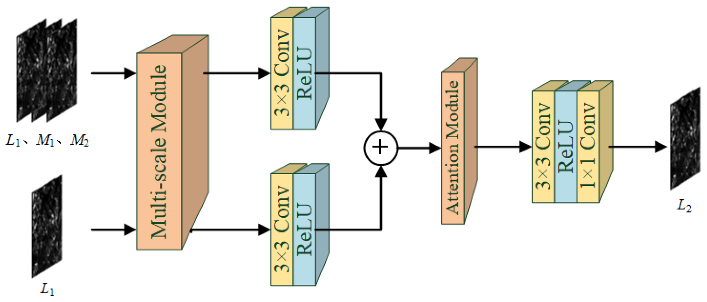
Figure 2 shows the spatiotemporal fusion network architecture proposed in this paper. The network is divided into two stages of input. The upper layer network input images are Landsat image L 1 at the reference time and a group of MODIS image pairs (MODIS image M 1 at the reference time and MODIS image M 2 at the prediction time). The input image of the lower layer network is the Landsat image L 1 at the reference time. For the convenience of illustration, we use “1 × 1 Conv” to represent the convolution layer with the convolutional kernel size of 1, “3 × 3 Conv” to represent the convolution layer with the convolution kernel size of 3, the activation function is ReLU, “multiscale module” represents the multiscale module, and “Attention Module” represents the attention-mechanism module. The multiscale-fusion features of the network are obtained from the input image through the multiscale module, and then the number of channels of the feature map is reduced through the convolution layer of 3 × 3. The features are merged by adding elements one by one, and then the fusion features are input into the attention module and reconstruction module; the reconstruction module is composed of a 3 × 3 convolution layer, an activation function ReLU and a 1 × 1 convolution layer. Finally, the feature map is reconstructed in the feature space to generate the Landsat-like image at the prediction time L 2 .

2.2.3. Multiscale Module

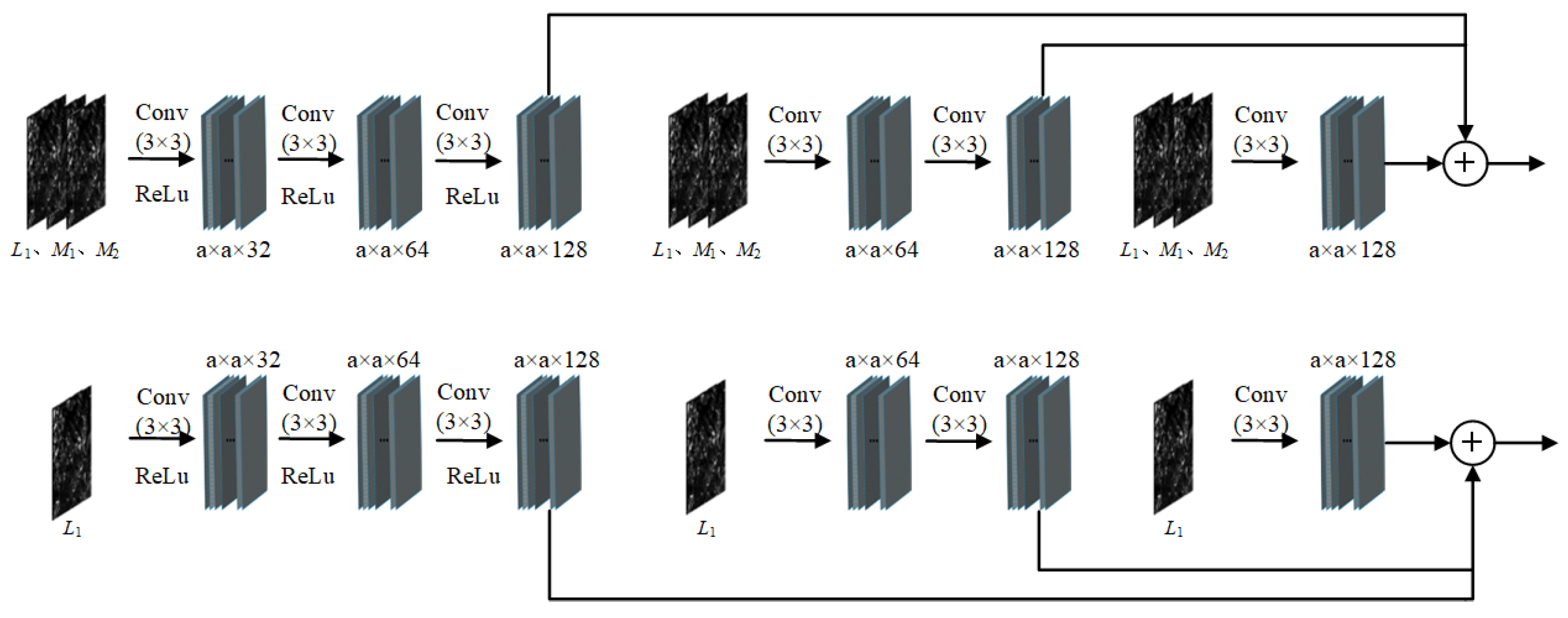
As remote-sensing images have features at different scales, the use of a single convolutional layer cannot fully extract all the features of images with rich feature information. Inspired by the target-detection model to solve the multiscale problem, this paper introduces multiscale feature fusion into the spatiotemporal fusion task. The multiscale fusion network is used to obtain the detail features of the input image at different scales; and then the obtained features are fused to obtain the fusion features at different scales; and, finally, the fusion features are processed. Therefore, the multiscale mechanism of Figure 3 is adopted to extract the spatial details and temporal variations from different scale images in the spatiotemporal fusion task. In Figure 3, Conv(3 × 3) represents the convolution layer with convolution kernel size of 3, and ReLu is used as the activation function of multiscale module. a × a × 32, a × a × 64, and a × a × 128 (length × width × number of channels), respectively, represent the dimensions of the convoluted feature graph. ⊕ indicates that the features are merged by adding the feature map element by element. The multiscale module proposed in this paper performs spatiotemporal fusion at three scales. For convenience of explanation, the input images L 1 , M 1 , and M 2 are denoted as M 12 , and L 1 is denoted as S 1 . μ i (i = 1, 2, 3) denotes convolution combination at different scales, F i (i = 1, 2, 3) denotes feature maps generated by convolution combination at different scales of input image M 12 , F denotes fusion features at multiple scales of input image M 12 , L i (i = 1, 2, 3) denotes feature maps generated by convolution combination at different scales of input image S 1 , and L denotes fusion features at multiple scales of input image S 1 . The process of multiscale module is as follows:
F 1 = μ 1 ( M 12 )
F 2 = μ 2 ( M 12 )
F 3 = μ 3 ( M 12 )
L 1 = μ 1 ( S 1 )
L 2 = μ 2 ( S 1 )
L 3 = μ 3 ( S 1 )
Finally, the fusion features of multiple scales are obtained by adding the feature maps element by element:
F = F 1 + F 2 + F 3
L = L 1 + L 2 + L 3

2.2.4. Attention Module

Attention mechanism is widely used in artificial-intelligence-related fields. It mainly utilizes the correlation between the data and also extracts the feature values according to their importance. The attention mechanism can guide the network to extract features towards the right direction. Hu et al. proposed that the squeeze-and-excitation network (SENet) [27] can help the network learn important channel feature information, which can improve the performance only by adding less computation. Subsequently, the block attention module (BAM) [28] and convolutional BAM (CBAM) [29] use multiple convolutions to extract the position information between features, but convolution can only obtain a large number of local features, and the comprehensive consideration of the whole image feature information is not comprehensive. The nonlocal approach [30] can obtain comprehensive spatial-feature information, but its huge overhead prevents it from becoming the mainstream and preferred method. The ideal method in this paper is to achieve both spatial attention and channel attention with less cost, and capture as much feature information as possible.
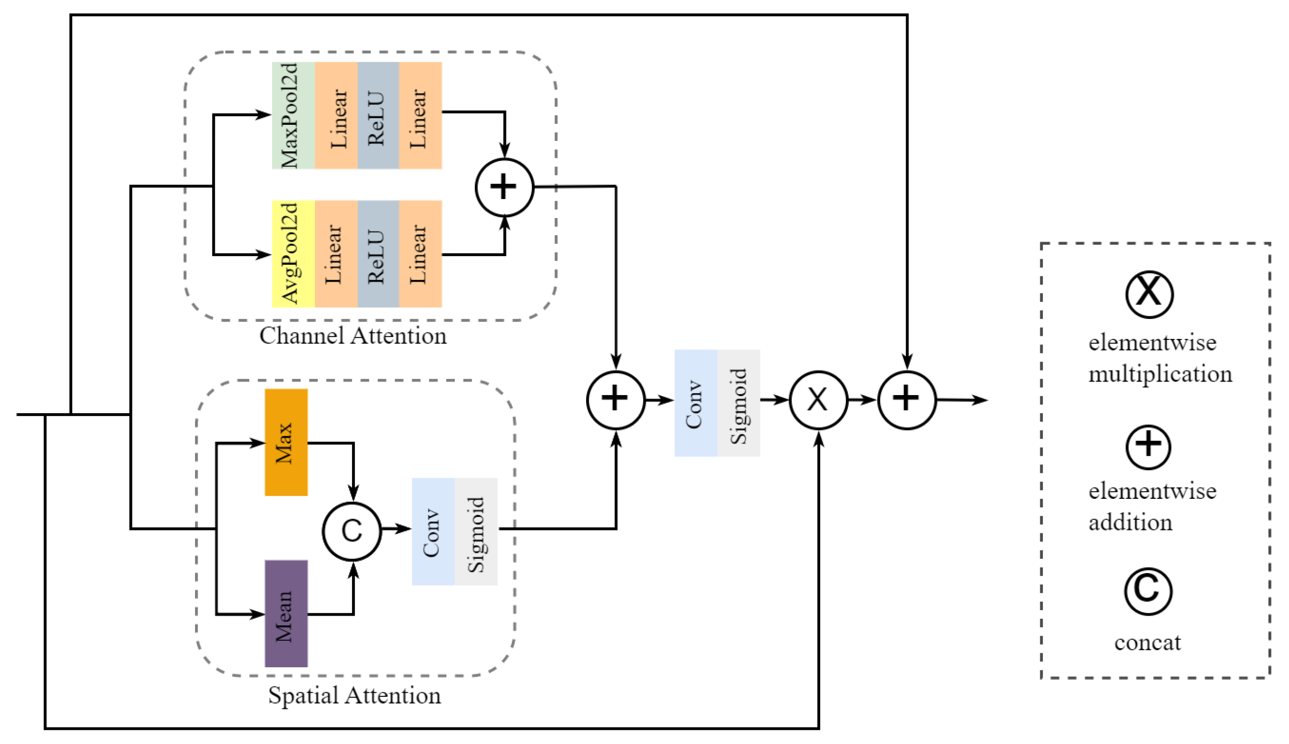
To solve the above problems, an efficient spatial-channel attention network is designed as shown in Figure 4. Averaging and maximizing the values of different channels on the same plane space enables obtaining the weights of spatial positions, connecting them for feature fusion, and then applying a convolution layer to finally generate spatial attention-feature map. In the two branches of channel attention mechanism, the average pooling layer and the maximum pooling layer are used to obtain the global statistical features of each input feature map, and then two full connection layers are used to generate channel features, that is, the optimal weight value of each feature channel is obtained from the relationship between the feature channels. Then, the two feature maps are merged by adding them element by element. Features passing through the spatial attention module and channel attention module are combined by adding feature maps element by element. Finally, through a 1 × 1 convolution layer and a Sigmoid layer, the weight value of the input feature passing through the spatial-channel attention module is obtained. The fusion features after local attention are obtained by shortcut connection. To accommodate the characteristics of CNN, the ReLU function is generally used as the activation function of each neuron in the fully connected layer, according to experience.
The feature information maps obtained by the spatial attention module and the channel attention module are integrated using convolutional layers and sigmoid functions, respectively, to obtain a more comprehensive feature information map. This process can be described as the following equation:
F o u t p u t = F i n p u t ( F i n p u t σ ( C o n v ( M c M s ) ) )
Here, F i n p u t and F o u t p u t , respectively, represent the input feature map and output feature map of the spatial-channel attention module; and M C and M S , respectively, represent the generated channel feature and spatial feature. Conv(·) and σ (·) represent convolution operations and Sigmoid function, respectively. ⨁ represents element-by-element addition, and ⨂ represents element-by-element multiplication function.

2.2.5. Compound Loss Function

The loss function has an important impact on the fusion results. In previous studies, the loss function generally used for image reconstruction is the l 2 loss function, which minimizes the loss and leads to the balance of errors between each pixel. This operation may lead to blurred images in spatiotemporal fusion results. The use of l 1 loss alone will, likewise, cause some interference in the generated fused images. Some previous attempts have been made to incorporate perceptual loss into their defined compound loss function [31]; however, perceptual loss must undergo a pre-training process, which is sensitive to the dataset and also incurs additional computational and time costs.
In order to address these current problems, this paper proposes a new compound loss function consisting of content loss, edge loss and visual loss, with the following equation:
L P r o p o s e d = L C o n t e n t + L E d g e + α · L V i s i o n ,
where α is the hyperparameter that regulates the visual loss, and, here, we empirically set it to 0.5. Content loss ( L C o n t e n t ) is a basic component of the compound loss function, a common practice in image fusion models, and is computed using the MSE.
L E d g e is a new edge loss proposed in this paper. In image-edge processing, the differential operation can highlight the image details and make the image clearer. Compared with the first-order differential operator, the second-order differential operator has stronger edge-positioning ability and better processing effect. Laplacian operator is the typical representative of the second-order differential operator, which is often used in the field of image enhancement and edge extraction [32]. The Laplacian operator is defined as in the following equation:
L a p l a c i a n ( f ) = 2 f x 2 2 f y 2
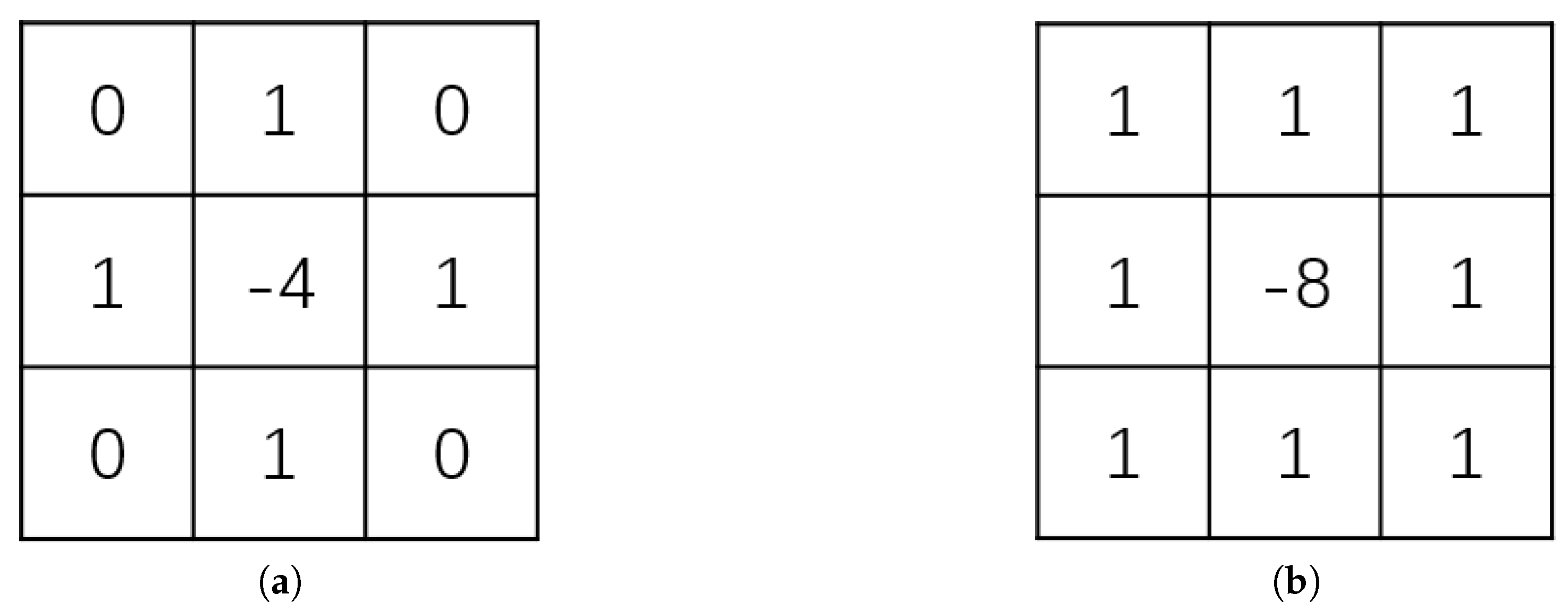
The Laplacian operator actually utilizes the Sobel operator [33]. It operates the derivatives in the x and y directions of the image by the Sobel operator to obtain the result of the Laplacian transform of the input image. The image in the neighborhood is calculated by the gray difference, and the Laplacian operator is divided into four neighborhoods and eight neighborhoods, as shown in Figure 5a,b. Four neighborhoods are gradients for four directions of the central pixel in the neighborhood, and eight neighborhoods are gradients for eight directions. In the implementation of the algorithm, Laplacian operator calculates gradients in four or eight directions of the central pixel in the neighborhood, and then adds up the gradients to judge the relationship between the gray level of the central pixel and the gray level of other pixels in the neighborhood. Finally, the gray level of pixels is adjusted through the result of gradient operation. The edge is characterized by a sudden change in intensity, which indicates the boundary between two regions of the image. With an ordinary gradient operator, it is difficult to determine the position of edge lines for steep edges and slowly changing edges, but Laplacian operator can be determined by the zero crossing point between the positive and negative peaks of quadratic differential, which is more sensitive to isolated points or endpoints [34]. Therefore, the method is particularly suitable for occasions with the purpose of highlighting isolated points, isolated lines or line end points in the image. Based on the above characteristics of Laplacian operator, this paper introduces Laplacian operator as edge loss to highlight the edge information of the image and obtain the fused image with clear edge-texture details. Specifically, the generated image and the real image are, respectively, subjected to Laplacian transform based on convolution operation, and the MSE is used to calculate the feature difference of the obtained image features, so as to obtain the edge loss of the predicted image and the real image. The Laplacian operator in this paper uses the edge repeated padding of padding 2 and the convolution kernel of 5 × 5. The edge loss function proposed in this paper can be expressed as the following equation:
L E d g e = 1 N i = 1 N ( ( F L t 1 ^ ) ( F L t 1 ) ) 2 ,
N represents the element of number of the feature map, · represents the Laplacian operation based on the convolution operation, F L t 1 ^ represents the predicted image, and F L t 1 represents real image.
Vision loss ( L V i s i o n ) is evaluated using the multiscale structural similarity (MS-SSIM) [35], which is often used in spatiotemporal image fusion models. The structural similarity (SSIM) is used to evaluate the degree of similarity between two images, mainly based on the similarity of brightness, contrast and overall structure of the images, which correspond to the image’s mean, standard deviation and correlation coefficient, respectively. SSIM can be expressed by Equation (14):
S S I M ( x , y ) = ( 2 μ x μ y + c 1 ) ( 2 σ x y + c 2 ) ( μ x 2 + μ y 2 + c 1 ) ( σ x 2 + σ y 2 + c 2 ) ,
where x and y represent the real image and the predicted image; μ x and μ y are recorded as the average value of x image and y image, respectively; σ x 2 and σ y 2 represent the variance in x image and y image, respectively. σ x y represents the covariance of the x and y images; c 1 and c 2 are used for stability equations. The value range of SSIM in image-reconstruction task is 0 to 1. The closer to 1. MS-SSIM, as a further expansion of SSIM, can still maintain better performance in different resolution images. The MS-SSIM is defined as shown in Equation (15):
L V i s i o n = 1 M S - S S I M
The research shows that MS-SSIM largely enables the high-frequency details in the input image to be retained in the fused image. Therefore, if MS-SSIM is included in the compound loss function, the fused image can be clearer.

2.3. Compared Methods

We selected five spatiotemporal fusion methods for comparison with our proposed method, namely, STARFM, flexible spatiotemporal data fusion (FSDAF) [3], and three deep-learning-based spatiotemporal fusion methods: DCSTFN, EDCSTFN, and AMNet. STARFM is a pixel reconstruction-based model, which assumes that the reflectance relationship between the low-resolution image and the high-resolution image is linear, so that multiple pixels of the high-resolution image corresponding to a pixel in the low-resolution image are from the same class. As long as this relationship is applied, the low-resolution image already acquired at the prediction date can be obtained as the high-resolution image at the prediction date. FSDAF predicts images more accurately by capturing progressive and abrupt land cover-class changes, and is applicable to heterogeneous regions. DCSTFN uses CNN to extract texture and spectral feature information from fine resolution images and coarse resolution images, respectively [18], and then uses the assumptions used by STARFM to synthesize the obtained feature information and fuse it into the final image. In contrast, EDCSTFN discards this assumption and obtains the fused image entirely through the autonomous learning capability of the network. It uses a compound loss function whichr includes a pretrained model; this will improve the fusion effect, but it also causes an increase in training-time cost and complexity. AMNet overlays multiple networks to generate fused images and uses an attention mechanism to improve the accuracy of the model, which has a good fusion effect.

2.4. Parameter Setting and Evaluation Strategy

The experiment sets the size of MODIS and Landsat image blocks to 400 × 400. Through many comparative tests on these parameters (i.e., 100, 120, 200, 300, 400), the sliding step is finally set to 200 × 200, so as to determine the best experimental results. In order to adapt to the limitation of GPU memory, the experiment set the training batch size to 4. We initialized the learning rate to 0.001 and chose 60 training rounds to let the model guarantee convergence. In addition, the learning rate varied with the training batches, and the loss value was reduced by 0.1 if it did not change after 5 consecutive epochs.
In this paper, a full range of comparisons was made between images observed by satellites and images generated according to spatiotemporal-fusion-methods comparison, including performance index and image color and texture. Regarding the evaluation of performance index, four indexes are used in this paper. The spatial correlation coefficient (SCC) reflects the linear correlation degree between the original image and the fused image. The closer the value of SCC is to 1, the greater the correlation of the two images. The SSIM reflects the structural similarity of the two comparison images in several aspects. Similarly, the values of SSIM of the two images show a positive correlation with their structural similarity. The larger SSIM, the stronger the structural similarity. The spectral angle mapper (SAM) [36] is the evaluation of the spectral similarity between images observed by satellites and images generated according to spatiotemporal fusion methods. The smaller the SAM, the more similar the two spectra are. Relative dimensionless comprehensive global error (ERGAS) [37] integrally evaluates the fusion results based on the prediction error, and the smaller the ERGAS, the better the results.

3. Results

3.1. Ablation Experiments

In this paper, ablation experiments were carried out on CIA and LGC datasets. Considering that different parts of the network may have different contributions to the network performance, the basic model (Baseline) was designed in this paper. In Baseline, the multiscale feature-fusion module in the network proposed in this paper was deleted, and the attention module is removed, and the edge loss function was deleted. We abbreviated the multiscale feature fusion module to Mu-scale, the spatial-channel attention module to Sp-Ca-Att, and the edge loss module to EgLoss. The final comparison results are shown in Table 1 and Table 2. “↑” indicates a higher value for a better quality image on that index, “↓” indicates a lower value for a better quality image on that index. The bolded numbers represent the best results.
For convenience of explanation, an id is given for each ablation experiment in this paper. Experiment 1 is the Baseline. In experiment 2, we added the edge loss module. Obviously, edge loss can improve the index performance of network models. The comparison results of experiment 3 show the effectiveness of an efficient space-channel attention module. It shows that the strategy of paying attention to spatial information and channel information is effective in the task of spatiotemporal fusion. Experiment 4 uses the multiscale feature-fusion module, which greatly improves the performance of the network fusion model. Finally, the multiscale spatiotemporal fusion network based on the attention mechanism proposed in this paper is presented. Comparing the experimental results of each module, it is shown that the proposed network in this paper can effectively make the spatiotemporal fusion task produce good results.
The decision coefficient R 2 can also be used to judge the predictive ability of the model, and its magnitude determines the closeness of the correlation. R 2 is mainly used to model two sets of data—in this case, the pixel values of the images—and then judge the degree of correlation of the two images based on the obtained correlation index and function. The formula is as follows.
R 2 = 1 i = 1 N ( x i y i ) 2 i = 1 N ( x i x ^ i ) 2 ,
where x ^ i represents the average pixel value of the observed image, y i represents the pixel value of the predicted image, x i represents the pixel value of the observed image, and N represents the total number of pixels in the image. The larger the value of R 2 , the better the fused image effect. Of course, the maximum value of R 2 is 1 and the minimum value is 0.
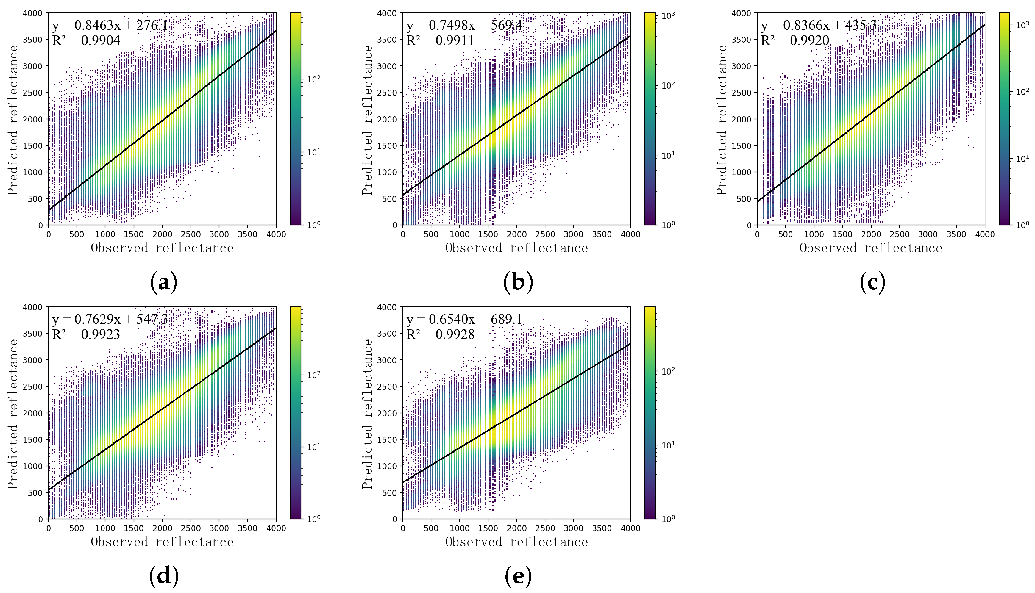
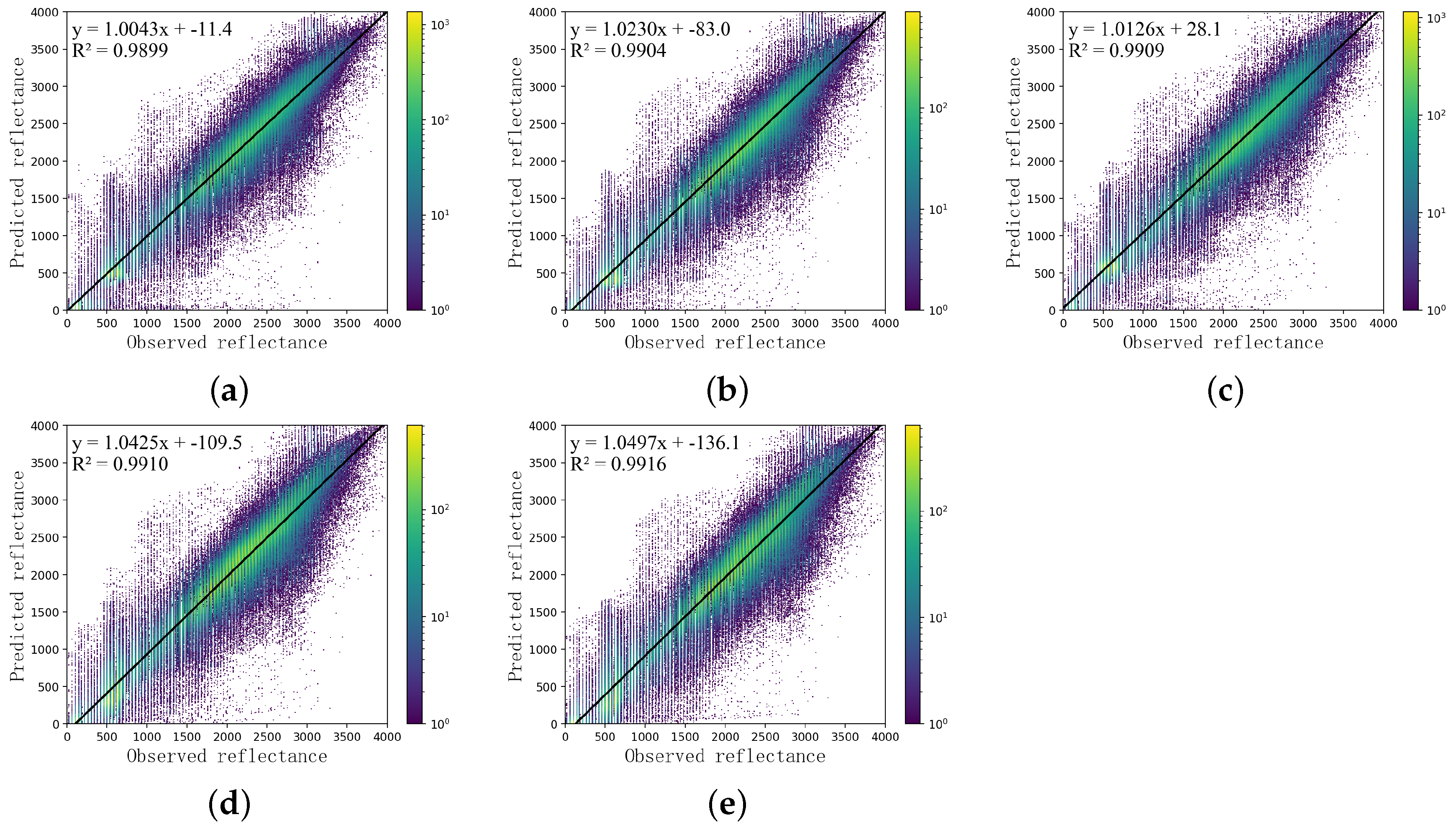
Figure 6 and Figure 7 show the closeness of the association between fusion images and real images in the near infrared (NIR) band of the LGC dataset and CIA dataset. The “point clouds” produced by each experiment differ only slightly, but the proposed method produces a higher concentration of “point clouds”, most of which are around the fitted straight line. There are also fewer scattered isolated points. At the same time, it can be jointly concluded that the fused image generated by the proposed network structure with complete modules is closer to the real image in relation to the R 2 value.

3.2. Comparative Experiments

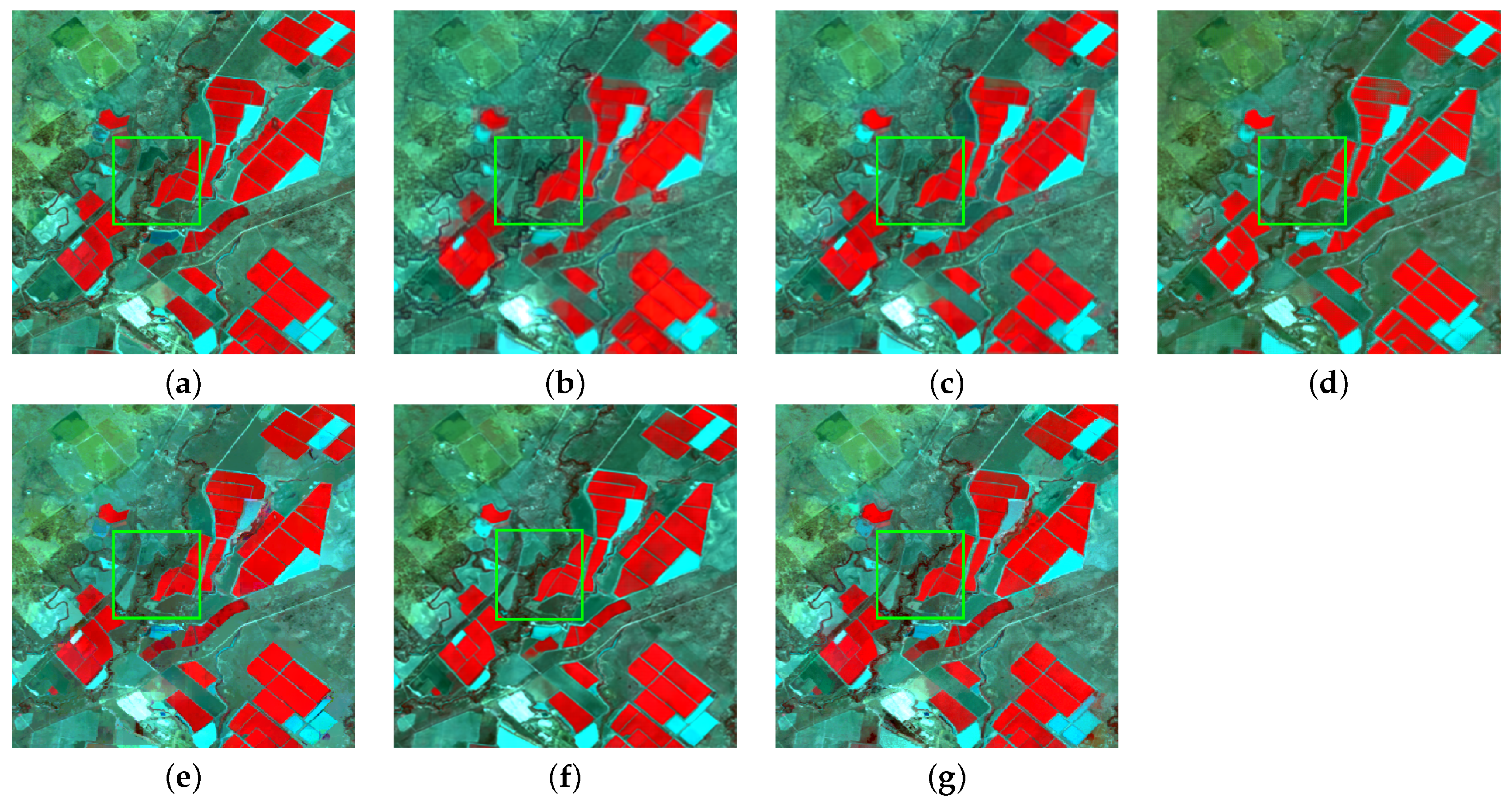
In this paper, the fusion image generated by each method under the same test case is preprocessed, and the local area of the fusion image is marked to show the effect of the fusion image more intuitively. The results of the CIA dataset on 4 May 2002 and the LGC dataset on 2 March 2005 are compared as shown in Figure 8 and Figure 9, respectively.
It can be seen from Figure 8 that on the CIA dataset, the overall structure of the image predicted by STARFM can still have local spectral inconsistencies. The FSDAF improves the expression of spectral quality; however, the details of local regions are blurred, for example, in the selected area where the edges of the contours are not clear enough. Compared with the four deep-learning methods, the DCSTFN and the EDCSTFN can predict some texture details in local regions, but the overall image quality is still not ideal. The overall spectral color of the AMNet fused image is darker and differs from the real image. The relatively high spatial heterogeneity of the CIA dataset leads to uncertainty in the variation in its corresponding image edges. Since the Laplacian operator in the proposed method in this paper may be disturbed by the uncertain variation in the image edges in the CIA dataset and the relatively smooth edge variation in the regions in the CIA dataset, achieving the further improvement of the effect of fused images is limited. It is still important for extracting the edge information of the images, as can also be seen from the subsequent experiments on the LGC dataset. In the image predicted by our proposed model, the texture details in local regions are further improved relative to the other three deep-learning methods. The overall visual effect of the performance is better, and the quality of the fused images is significantly better than other algorithms.
Figure 9 shows the performance of each fusion algorithm in the LGC dataset. The LGC dataset is less heterogeneous, so the quality of the generated fused images performs better than the CIA dataset. Compared with the two traditional methods, the texture edge details in the local regions are blurred, and there are more obvious areas of color distortion. Three other deep-learning methods and the method proposed in this paper predict rich texture details and express spectral information well. AMNet performs quite well on the LGC dataset. Of course, the fusion effect of the method proposed in this paper is also good.
In addition to the comparison in terms of objective visualization, this paper also provides a quantitative comparison of the performance of the methods in terms of index. The image index obtained at multiple time points are averaged to obtain the final value of the corresponding method on that index. Table 3 and Table 4 represent the index performance of each method on the CIA dataset and LGC dataset, where we show the best performing index in bold black font.
It can be seen from Table 3 and Table 4 that our proposed method also has the best index performance among the comparison methods. The STARFM and FSDAF performed similarly. The EDCSTFN has a great improvement in spectral index and structural similarity, and the SSIM index of EDCSTFN is 2.3% higher than that of STARFM on the CIA dataset, and the method proposed in this paper is superior to these five methods in all indexes.
Table 5 shows the computational efficiency of the three deep-learning methods. We evaluated the computational efficiency (FLOPs) of the deep-learning-based models in terms of both number of parameters and floating points of operations (FLOPs). The G in FLOPs(G) stands for 1 × 10 6 , and FLOPs are mainly used to measure the complexity of the model in an integrated manner. As can be seen from Table 5, because EDCSTFN requires training of a pretrained model, the number of required parameters is relatively large and the model complexity is not low. Taken together, the method proposed in this paper is more efficient than DCSTFN, EDCSTFN and AMNet in terms of computational efficiency, indicating its better computational performance.

3.3. Residual Experiments

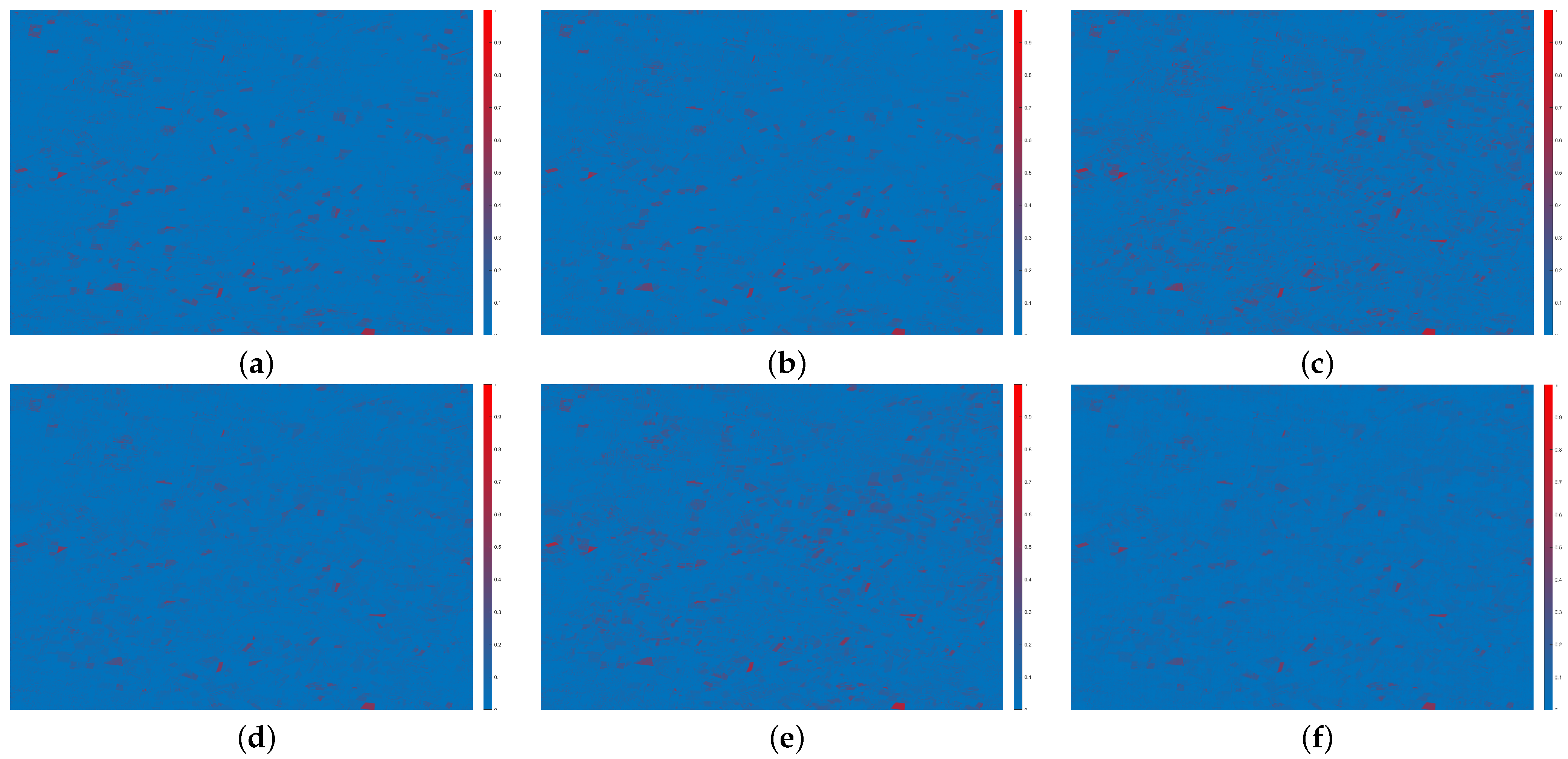
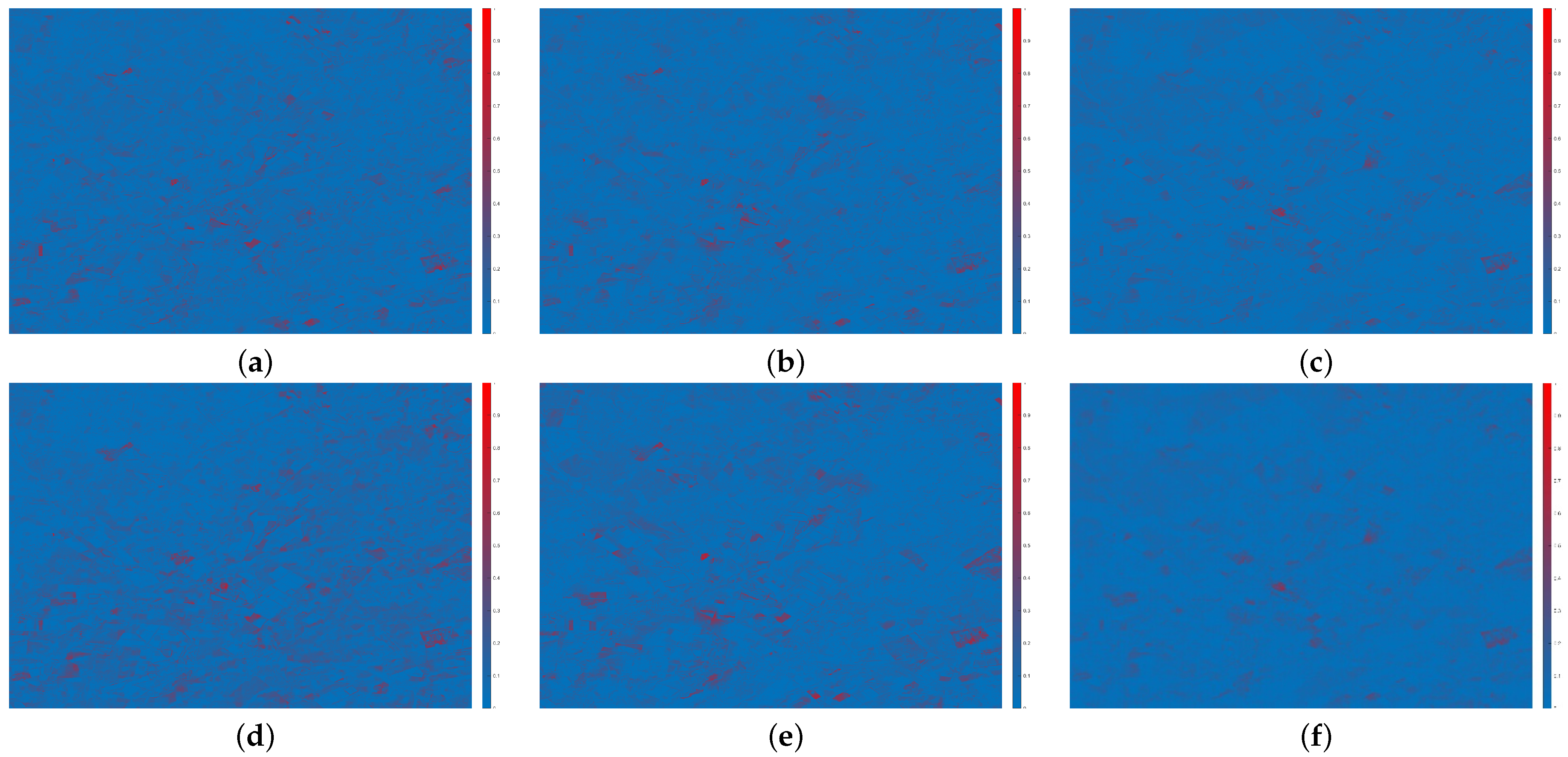
In order to visualize the experimental index obtained in the comparison experiments, residual experiments were conducted in this paper. The process of the residual experiment is to average the number obtained by subtracting each band of the fused image from the real image to obtain an image with all bands. Finally, this fused image is then normalized. As shown in Figure 10 and Figure 11, the larger and deeper the blue area in the image, the smaller the difference between the predicted image and the real image, and the better the fusion effect. Obviously, the results obtained by the STARFM is relatively poor, with a large number of red and black regions. FSDAF has fewer red and black areas and its effect is better than STARFM. In the deep-learning method, the red and black regions of EDCSTFN are significantly reduced, indicating that the quality of the fused image is significantly improved compared with the traditional methods. Compared with EDCSTFN, the fused image generated by the network proposed in this paper has the most blue areas, indicating that it has the best fusion.

4. Discussion

The experimental results on the CIA and LGC datasets show that the proposed spatiotemporal fusion method is superior to the five new spatiotemporal fusion methods. Its advantages are summarized as follows:
  • Whether for LGC dataset with high image quality or CIA dataset with slightly poor image quality, the model proposed in this paper can still maintain good performance, which shows that it has better robustness. This is due to the use of multiscale feature fusion to obtain the spatial details and temporal changes in the input image at different scales. At the same time, the spatial-channel attention module also filters the unimportant features for the network in the learning process, so that the required features can be better expressed.
  • The edge loss designed in this paper is proven to be effective on the CIA dataset and LGC dataset, which can improve the learning and optimization ability of the network, make the fused image show more abundant texture details, and avoid the additional computational cost and time cost in obtaining the perceptual loss training pre-training model, thus saving a lot of computational resources.

5. Conclusions

In this paper, a multiscale spatiotemporal fusion network based on an attention mechanism is proposed. Multiscale feature fusion is introduced into the spatiotemporal fusion task to obtain the spatial details and temporal changes in remote-sensing images at different scales for the purpose of extracting richer and more comprehensive feature information. A spatial-channel attention module is used to filter the spatial features and channel information of the fusion network in order to obtain more important feature information. The edge loss function is added and incorporated into the compound loss function to reduce the overhead and complexity of the network and further improve the prediction accuracy and the quality of the fused images. The effectiveness of the proposed network is verified by the results of an ablation experiment and comparative experiment. In addition, from the comparison of the residual diagrams, it can be concluded that, in the spectral performance, our proposed method shows more blue regions with the value of 0, showing the great advantage of our proposed model. Taken together, our method clearly outperforms STARFM, DCSTFN, EDCSTFN and AMNet, and our method has a more accurate prediction capability with a richer expression of spectral information. The combination of images and indexes shows that our proposed method achieves good results in both subjective visual and objective evaluation. However, the performance in terms of details needs to be improved. This is because we found that the model is able to predict better the texture edge information in the region with more spectral color information, but at the same time the expression of the spectral information in that part is biased. The follow-up study found that the strong edge structure of the edge-extraction operator we used may cause the model to focus too much on the structural information and ignore the expression of the spectral information. Future work needs to focus on structural information while paying attention to the expression of spectral information, and, in the meantime, the feasibility of applying other edge operators to spatiotemporal fusion tasks needs to be explored. In addition, in view of the better performance shown by traditional methods, the combination of traditional methods and deep-learning methods can also be explored in the future, to further improve the quality of image fusion.

Author Contributions

Conceptualization, D.L.; methodology, M.B. and Z.H.; data curation, Z.H. and M.B.; funding acquisition, D.L.; investigation, L.Z.; project administration, D.L.; software, Q.W. and Q.G.; visualization, Z.M.; supervision, D.L.; validation, Y.L. and D.L.; writing—original draft preparation, M.B. and Z.H.; writing—review and editing, D.L. and Y.L. All authors have read and agreed to the published version of the manuscript.

Funding

This work was supported by the National Natural Science Foundation of China (Nos. 61972060, U1713213 and 62027827), National Key Research and Development Program of China (No. 2019YFE0110800), Natural Science Foundation of Chongqing (Nos. cstc2020jcyj-zdxmX0025, cstc2019cxcyljrc-td0270).

Institutional Review Board Statement

Not applicable.

Informed Consent Statement

Not applicable.

Data Availability Statement

The data presented in this study are available on request from the corresponding author. The data are not publicly available due to the fact that the data has been pre-processed and involves laboratory intellectual property rights.

Acknowledgments

The authors would like to thank all members of Chongqing Key Laboratory of Image Cognition for their kindness and help.

Conflicts of Interest

The authors declare no conflict of interest.

Abbreviations

The following abbreviations are used in this manuscript:
HTLSHigh temporal but low spatial resolution
LTHSLow temporal but high spatial resolution
MODISModerate resolution imaging spectrometer
STARFMSpatial and temporal adaptive reflectance fusion model
FSDAFFlexible spatiotemporal data fusion approach
STAARCHSpatial and temporal adaptive algorithm for mapping reflectance changes
CNNConvolutional neural network
DCSTFNDeep convolutional spatiotemporal fusion network
STFDCNNSpatiotemporal fusion using deep convolutional neural networks
SRCNNSingle-image superresolution convolutional neural network
StfNetTwo-stream convolutional neural network
EDCSTFNEnhanced deep convolutional spatiotemporal fusion network
AMNetConvolutional neural network with attention and multiscale mechanisms
SENetSequeeze-and-excitation network
BAMBlock attention module
CBAMConvolutional block attention module
STNSpatial transformer network
SSIMStructural similarity
MS-SSIMMultiscale structural similarity
LGCLower Gwydir Catchment
CIAColeambally Irrigation Area
TMLandsat-5 Thematic Map
ETM+Landsat-7 Enhanced Thematic Mapper Plus
SCCSpatial correlation coefficient
SAMSpectral angle mapper
ERGASRelative dimensionless comprehensive global error

References

  1. Toth, C.K.; Jóźków, G. Remote sensing platforms and sensors: A survey. ISPRS J. Photogramm. Remote Sens. 2016, 115, 22–36. [Google Scholar] [CrossRef]
  2. Arévalo, P.; Olofsson, P.; Woodcock, C.E. Continuous monitoring of land change activities and post-disturbance dynamics from Landsat time series: A test methodology for REDD+ reporting. Remote Sens. Environ. 2020, 238, 111051. [Google Scholar] [CrossRef]
  3. Zhu, X.; Helmer, E.H.; Gao, F.; Liu, D.; Chen, J.; Lefsky, M.A. A flexible spatiotemporal method for fusing satellite images with different resolutions. Remote Sens. Environ. 2016, 172, 165–177. [Google Scholar] [CrossRef]
  4. Chen, B.; Huang, B.; Xu, B. Comparison of Spatiotemporal Fusion Models: A Review. Remote Sens. 2015, 7, 1798–1835. [Google Scholar] [CrossRef] [Green Version]
  5. Belgiu, M.; Stein, A. Spatiotemporal Image Fusion in Remote Sensing. Remote Sens. 2019, 11, 818. [Google Scholar] [CrossRef] [Green Version]
  6. Roy, D.P.; Wulder, M.A.; Loveland, T.R.; Woodcock, C.E.; Allen, R.G.; Anderson, M.C.; Helder, D.L.; Irons, J.R.; Johnson, D.M.; Kennedy, R.E.; et al. Landsat-8: Science and Product Vision for Terrestrial Global Change Research. Remote Sens. Environ. 2014, 145, 154–172. [Google Scholar] [CrossRef] [Green Version]
  7. Justice, C.O.; Vermote, E.F.; Townshend, J.R.; DeFries, R.S.; Roy, D.P.; Hall, D.K.; Salomonson, V.V.; Privette, J.L.; Riggs, G.A.; Strahler, A.H.; et al. The Moderate Resolution Imaging Spectroradiometer (MODIS): Land remote sensing for global change research. IEEE Trans. Geosci. Remote Sens. 1998, 36, 1228–1249. [Google Scholar] [CrossRef] [Green Version]
  8. Tan, Z.; Yue, P.; Di, L.; Tang, J. Deriving High Spatiotemporal Remote Sensing Images Using Deep Convolutional Network. Remote Sens. 2018, 10, 1066. [Google Scholar] [CrossRef] [Green Version]
  9. Li, W.; Yang, C.; Peng, Y.; Zhang, X. A Multi-Cooperative Deep Convolutional Neural Network for Spatiotemporal Satellite Image Fusion. IEEE J. Sel. Top. Appl. Earth Obs. Remote Sens. 2021, 14, 10174–10188. [Google Scholar] [CrossRef]
  10. Yokoya, N.; Grohnfeldt, C.; Chanussot, J. Hyperspectral and Multispectral Data Fusion: A comparative review of the recent literature. IEEE Geosci. Remote Sens. Mag. 2017, 5, 29–56. [Google Scholar] [CrossRef]
  11. Gao, F.; Masek, J.G.; Schwaller, M.R.; Hall, F.G. On the blending of the Landsat and MODIS surface reflectance: Predicting daily Landsat surface reflectance. IEEE Trans. Geosci. Remote Sens. 2006, 44, 2207–2218. [Google Scholar]
  12. Hilker, T.; Wulder, M.A.; Coops, N.C.; Linke, J.; McDermid, G.J.; Masek, J.G.; Gao, F.; White, J.C. A new data fusion model for high spatial- and temporal-resolution mapping of forest disturbance based on Landsat and MODIS. Remote Sens. Environ. 2009, 113, 1613–1627. [Google Scholar] [CrossRef]
  13. Chen, J.; Pan, Y.; Chen, Y. Remote sensing image fusion based on Bayesian GAN. arXiv 2020, arXiv:2009.09465. [Google Scholar]
  14. Huang, B.; Zhang, H.K.; Song, H.; Wang, J.; Song, C. Unified fusion of remote-sensing imagery: Generating simultaneously high-resolution synthetic spatial–temporal–spectral earth observations. Remote Sens. Lett. 2013, 4, 561–569. [Google Scholar] [CrossRef]
  15. Li, A.; Li, A.; Bo, Y.; Bo, Y.; Zhu, Y.; Zhu, Y.; Guo, P.; Guo, P.; Bi, J.; Bi, J.; et al. Blending multi-resolution satellite sea surface temperature (SST) products using Bayesian maximum entropy method. Remote Sens. Environ. 2013, 135, 52–63. [Google Scholar] [CrossRef]
  16. Peng, Y.; Li, W.; Luo, X.; Du, J.; Zhang, X.; Gan, Y.; Gao, X. Spatiotemporal Reflectance Fusion via Tensor Sparse Representation. IEEE Trans. Geosci. Remote Sens. 2022, 60, 1–18. [Google Scholar] [CrossRef]
  17. Song, H.; Liu, Q.; Wang, G.; Hang, R.; Huang, B. Spatiotemporal Satellite Image Fusion Using Deep Convolutional Neural Networks. IEEE J. Sel. Top. Appl. Earth Obs. Remote Sens. 2018, 11, 821–829. [Google Scholar] [CrossRef]
  18. Jia, D.; Song, C.; Cheng, C.; Shen, S.; Ning, L.; Hui, C. A Novel Deep Learning-Based Spatiotemporal Fusion Method for Combining Satellite Images with Different Resolutions Using a Two-Stream Convolutional Neural Network. Remote Sens. 2020, 12, 698. [Google Scholar] [CrossRef] [Green Version]
  19. Schmidhuber, J. Deep learning in neural networks: An overview. Neural Netw. Off. J. Int. Neural Netw. Soc. 2015, 61, 85–117. [Google Scholar] [CrossRef] [Green Version]
  20. Liu, X.; Deng, C.; Chanussot, J.; Hong, D.; Zhao, B. StfNet: A Two-Stream Convolutional Neural Network for Spatiotemporal Image Fusion. IEEE Trans. Geosci. Remote Sens. 2019, 57, 6552–6564. [Google Scholar] [CrossRef]
  21. Tan, Z.; Di, L.; Zhang, M.; Guo, L.; Gao, M. An Enhanced Deep Convolutional Model for Spatiotemporal Image Fusion. Remote Sens. 2019, 11, 2898. [Google Scholar] [CrossRef] [Green Version]
  22. Li, W.; Zhang, X.; Peng, Y.; Dong, M. Spatiotemporal Fusion of Remote Sensing Images using a Convolutional Neural Network with Attention and Multiscale Mechanisms. Int. J. Remote Sens. 2020, 42, 1973–1993. [Google Scholar] [CrossRef]
  23. Yin, S.; Li, H.; Teng, L.; Jiang, M.; Karim, S. An optimised multi-scale fusion method for airport detection in large-scale optical remote sensing images. Int. J. Image Data Fusion 2020, 11, 201–214. [Google Scholar] [CrossRef]
  24. Lai, Z.; Chen, L.; Jeon, G.; Liu, Z.; Zhong, R.; Yang, X. Real-time and effective pan-sharpening for remote sensing using multi-scale fusion network. J. Real Time Image Process. 2021, 18, 1635–1651. [Google Scholar] [CrossRef]
  25. Zhang, C.; Chen, Y.; Yang, X.; Gao, S.; Li, F.; Kong, A.; Zu, D.; Sun, L. Improved Remote Sensing Image Classification Based on Multi-Scale Feature Fusion. Remote Sens. 2020, 12, 213. [Google Scholar] [CrossRef] [Green Version]
  26. Emelyanova, I.; McVicar, T.R.; van Niel, T.G.; Li, L.; van Dijk, A.I.J.M. Assessing the accuracy of blending Landsat–MODIS surface reflectances in two landscapes with contrasting spatial and temporal dynamics: A framework for algorithm selection. Remote Sens. Environ. 2013, 133, 193–209. [Google Scholar] [CrossRef]
  27. Hu, J.; Shen, L.; Sun, G. Squeeze-and-Excitation Networks. In Proceedings of the 2018 IEEE/CVF Conference on Computer Vision and Pattern Recognition, Salt Lake City, UT, USA, 18–23 June 2018; pp. 7132–7141. [Google Scholar]
  28. Park, J.; Woo, S.; Lee, J.Y.; Kweon, I.S. BAM: Bottleneck Attention Module. In Proceedings of the BMVC, Newcastle, UK, 3–6 September 2018. [Google Scholar]
  29. Woo, S.; Park, J.; Lee, J.Y.; Kweon, I.S. CBAM: Convolutional Block Attention Module. In Proceedings of the ECCV, Munich, Germany, 8–14 September 2018. [Google Scholar]
  30. Mei, Y.; Fan, Y.; Zhou, Y. Image Super-Resolution with Non-Local Sparse Attention. In Proceedings of the 2021 IEEE/CVF Conference on Computer Vision and Pattern Recognition (CVPR), Nashville, TN, USA, 20–25 June 2021; pp. 3516–3525. [Google Scholar]
  31. Johnson, J.; Alahi, A.; Fei-Fei, L. Perceptual Losses for Real-Time Style Transfer and Super-Resolution. arXiv 2016, arXiv:1603.08155. [Google Scholar]
  32. Wang, X. Laplacian Operator-Based Edge Detectors. IEEE Trans. Pattern Anal. Mach. Intell. 2007, 29, 886–890. [Google Scholar] [CrossRef]
  33. Lei, D.; Bai, M.; Zhang, L.; Li, W. Convolution neural network with edge structure loss for spatiotemporal remote sensing image fusion. Int. J. Remote Sens. 2022, 43, 1015–1036. [Google Scholar] [CrossRef]
  34. Tian, Q.; Xie, G.; Wang, Y.; Zhang, Y. Pedestrian detection based on laplace operator image enhancement algorithm and faster R-CNN. In Proceedings of the 2018 11th International Congress on Image and Signal Processing, BioMedical Engineering and Informatics (CISP-BMEI), Beijing, China, 13–15 October 2018; IEEE: Piscataway, NJ, USA, 2018; pp. 1–5. [Google Scholar]
  35. Zhao, H.; Gallo, O.; Frosio, I.; Kautz, J. Loss Functions for Neural Networks for Image Processing. arXiv 2015, arXiv:1511.08861. [Google Scholar]
  36. Yuhas, R.H.; Goetz, A.F.H.; Boardman, J.W. Discrimination among semi-arid landscape endmembers using the Spectral Angle Mapper (SAM) algorithm. In Proceedings of the Third Annual JPL Airborne Geoscience Workshop, Pasadena, CA, USA, 1–5 June 1992. [Google Scholar]
  37. Khan, M.M.; Alparone, L.; Chanussot, J. Pansharpening Quality Assessment Using the Modulation Transfer Functions of Instruments. IEEE Trans. Geosci. Remote Sens. 2009, 47, 3880–3891. [Google Scholar] [CrossRef]
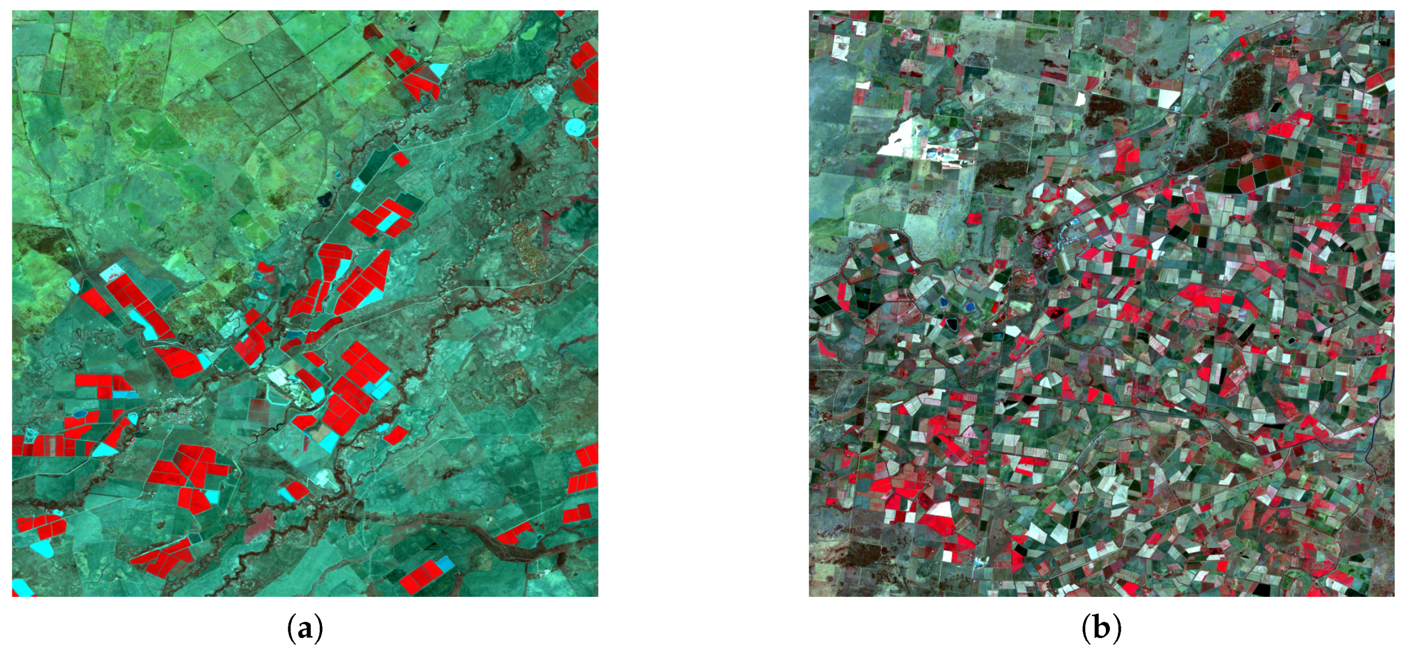
Figure 1. Real Landsat images of (a) LGC dataset and (b) CIA dataset.
Remotesensing 15 00182 g001
Figure 2. Network architecture diagram.
Remotesensing 15 00182 g002
Figure 3. Multiscale feature-fusion module.
Remotesensing 15 00182 g003
Figure 4. Efficient spatial-channel attention module.
Remotesensing 15 00182 g004
Figure 5. (a) Four-neighbor template and (b) eight-neighbor template.
Remotesensing 15 00182 g005
Figure 6. Correlation between the NIR band predicted image and real image on 4 May 2002 of CIA. (a) baseline. (b) baseline + Egloss. (c) baseline + Sp-Ca-Att. (d) baseline + Mu-scale. (e) proposed.
Remotesensing 15 00182 g006
Figure 7. Correlation between NIR band predicted image and real image on 2 March 2005 of LGC. (a) baseline. (b) baseline + Egloss. (c) baseline + Sp-Ca-Att. (d) baseline + Mu-scale. (e) proposed.
Remotesensing 15 00182 g007
Figure 8. CIA dataset of real image acquired on 4 May 2002 and predicted images generated by each fusion method. (a) Observed. (b) STARFM. (c) FSDAF. (d) DCSTFN. (e) EDCSTFN. (f) AMNet. (g) Proposed method.
Remotesensing 15 00182 g008
Figure 9. LGC dataset of real image acquired on 2 March 2005 and predicted images generated by each fusion method. (a) Observed. (b) STARFM. (c) FSDAF. (d) DCSTFN. (e) EDCSTFN. (f) AMNet. (g) Proposed method.
Remotesensing 15 00182 g009
Figure 10. Comparison of the residual diagrams produced by various methods for the CIA dataset on 4 May 2002. (a) STARFM. (b) FSDAF. (c) DCSTFN. (d) EDCSTFN. (e) AMNet. (f) The proposed method.
Remotesensing 15 00182 g010
Figure 11. Comparison of the residual diagrams produced by various methods for the LGC dataset on 2 March 2005. (a) STARFM. (b) FSDAF. (c) DCSTFN. (d) EDCSTFN. (e) AMNet. (f) The proposed method.
Remotesensing 15 00182 g011
Table 1. Performance of different modules on the CIA dataset.
IDBaselineMu-ScaleSp-Ca-AttEglossSAMERGASSCCSSIM
1 4.81181.30490.80810.6484
2 4.61011.28530.81250.6824
3 4.42511.29890.82530.6983
4 4.32541.24580.82040.7015
53.80571.08870.83620.7372
Reference
Table 2. Performance of different modules on the LGC dataset.
IDBaselineMu-ScaleSp-Ca-AttEglossSAMERGASSCCSSIM
1 4.49700.97360.86810.7695
2 4.38540.95470.86910.7724
3 4.36120.95630.87640.7687
4 4.26770.92430.87420.7802
54.12280.91650.88880.7948
Reference
Table 3. Index performance of each method on the CIA dataset.
MethodSAMERGASSCCSSIM
STARFM4.92891.49400.81530.6947
FSDAF4.54971.36510.80750.7021
DCSTFN4.22941.16180.81210.7093
EDCSTFN4.89311.14480.81820.7193
AMNet4.16981.26460.82230.6975
Proposed3.80571.08870.83620.7372
Reference0011
Table 4. Index performance of each method on the LGC dataset.
MethodSAMERGASSCCSSIM
STARFM4.56731.16850.87180.7829
FSDAF4.58911.23070.86610.7789
DCSTFN5.36621.08750.84570.6924
EDCSTFN4.56491.06010.87500.7843
AMNet4.80681.27810.88560.7905
Proposed4.11280.91650.88880.7948
Reference0011
Table 5. Comparison of computational efficiency of each method.
MethodParametersFLOPs(G)
DCSTFN408,961150.481
EDCSTFN762,856111.994
AMNet633,45297.973
Proposed176,23736.846
Reference
Disclaimer/Publisher’s Note: The statements, opinions and data contained in all publications are solely those of the individual author(s) and contributor(s) and not of MDPI and/or the editor(s). MDPI and/or the editor(s) disclaim responsibility for any injury to people or property resulting from any ideas, methods, instructions or products referred to in the content.