A Multi-View Thermal–Visible Image Dataset for Cross-Spectral Matching

Abstract

Cross-spectral local feature matching between visual and thermal images benefits many vision tasks in low-light environments, including image-to-image fusion and camera re-localization. An essential prerequisite for unleashing the potential of supervised deep learning algorithms in the area of visible–thermal matching is the availability of large-scale and high-quality annotated datasets. However, publicly available datasets are either in relative small quantity scales or have limited pose annotations due to the expensive cost of data acquisition and annotation, which severely hinders the development of this field. In this paper, we proposed a multi-view thermal–visible image dataset for large-scale cross-spectral matching. We first recovered a 3D reference model from a group of collected RGB images, in which a certain image (bridge) shares almost the same pose as the thermal query. We then effectively registered the thermal image to the model based on manually annotating a 2D-2D tie point between the bridge and the thermal. In this way, through simply annotating one same viewpoint image pair, numerous overlapping image pairs between thermal and visible could be available. We also proposed a semi-automatic approach for generating accurate supervision for training multi-view cross-spectral matching. Specifically, our dataset consists of 40,644 cross-modal pairs with well supervision, covering multiple complex scenes. In addition, we also provided the camera metadata, 3D reference model, depth map of the visible images and 6-DoF pose of all images. We extensively evaluated the performance of state-of-the-art algorithms on our dataset and provided a comprehensive analysis of the results. We will publish our dataset and pre-processing code.

1. Introduction

Thermal and visible image matching is the problem of estimating local feature correspondences between cross-spectral images. Cross-spectral matching is a core component of many interesting applications in low-light conditions, such as infrared-and-visible information fusion, scene-level drone navigation, and autonomous driving at night.

Surprisingly, we notice that, while the ongoing revolution in data-driven deep network has boosted the performance of visible-to-visible matching, tradition descriptors such as SIFT [1] still dominate the field of thermal-to-visible correspondence estimation. However, it is important to state that adopting handcrafted features usually leads to an unsatisfying result, as cross-domain images share a notable difference in color and texture due to inconsistent imaging mechanisms and capturing sensors. We believe that the main reason for the absence of learning-based approaches in the field is the lack of large-scale and well-annotated training datasets. This is mainly because, unlike visible-only datasets such as Megadepth [2] and ScanNet [3], the data acquisition and annotation for two-source images is much more difficult. Manually labeling cross-domain correspondences for thousands of image pairs will put a heavy burden on human and financial resources. As a result, the existing thermal–visible datasets generally belong to two kinds: (1) small-scale benchmark datasets [4,5] and (2) large-scale image-fusion datasets [6]. The first category usually includes just a few dozen items, which can only be used to test the classic algorithm. The second category, however, contains tens of thousands of photos that only cover some single scenes and fixed viewpoints, which is also subpar when training neural networks, especially for geometric tasks.

To this end, we aimed to establish a new paradigm for thermal–visible image matching that incorporates the following three characteristics. Firstly, our dataset should have a sufficient number of matched pairs ranging in various scenes. Data abundance significantly contributes to improving the quality of the trained model. Secondly, multi-view pairs are necessary for geometric-related tasks such as camera re-localization. The reason for this is that, during the real navigation process in low-light conditions, the query thermal photo always shares a different viewpoint to reference day-time RGB images. Thirdly, manual annotation needs to be minimized considering the economic and efficiency factors.

In this paper, we proposed a multi-view thermal–visible matching dataset (called MTV), which consisted of three stages: data acquisition, 3D model reconstruction, and supervision generation. In the first stage, we used a quadcopter drone (DJI M300 RTK) that was equipped with an oblique five-eye camera for day and a multi-sensors camera for night, respectively, in order to stably capture aerial image sequences. The key to data collection is to obtain many visible (day-time) and thermal (night-time) image pairs with basically the same viewpoint. Thanks to the precise Waypoint function of DJI M300 RTK, we can obtain thermal–visible image pairs with almost the same poses, which improves the efficiency of manual annotation. We refer to such visible light images as the “bridge”. This played a crucial role in building our dataset. We manually matched the bridge–thermal image pair to obtain the absolute pose of the thermal image, while the bridge image helps the thermal image retrieve a large number of cross-view visible images with overlapping regions. In the second stage, we used the offline system COLMAP [7] to perform camera pose recovery and reconstruct the reference 3D model for all visible light aerial images taken during the day. The 3D point cloud and Pose helped us to establish the pixel-wise correspondence between thermal–visible by means of projection in later steps. In the final stage, we registered the thermal image to the pre-built 3D model through manually annotating the tie point of the same-perspective bridge–thermal pair. We also proposed a semi-automatic approach for generating the supervision, with human guidance, to boost the efficiency and provide a large number of corresponding points. In addition, we also provided the absolute pose of all images, accompanied and georeferenced with GPS and flight altitude information, which can be applied to the georeferenced localization algorithms.

In summary, this paper makes the following contributions:

• We published a multi-view thermal–visible matching dataset, where the thermal and visible images are no longer restricted to the same viewpoint, which is particularly important for training geometric-based matching algorithms.
• We proposed a novel semi-automatic supervision generation approach for thermal–visible matching dataset construction that generates numerous image pairs for deep networks with affordable manual intervention.
• All thermal and visible images are accompanied by an accurate georeference, which can be used to evaluate localization algorithms.
• Compared to the previous dataset, we increased the number of image pairs by many times and included various challenging scenes.

2. Related Work

2.1. Thermal–Visible Datasets

Existing thermal–visible datasets can be broadly classified into two categories based on whether the viewpoint is fixed. For single-view datasets, OSU Color [8], TNO Fusion [5], INO Videos, VLIRVDIF [9], VIFB [4], and LLVIP [6] are included. Specifically, OSU [8] focuses on the fusion of color and thermal imagery and, next, fusion-based object detection. However, all images are collected during the daytime, in which, the advantage of thermal imaging is not prominent. TNO [5] is the most commonly used public dataset for visible and infrared image fusion. Unfortunately, TNO [5] only contains 63 pairs of images, which makes it hard to train the neural network. The same problem happens in INO [10] Videos and VIFB [4] datasets, where the small pair number is not enough to support the model supervision. VLIRVDIF [9] is a visible-light and infrared video database for information fusion, but it does not provide camera-intrinsic parameters. Aguilera et al. provided a visual-thermal dataset named Barcelona [11]. The Barcelona dataset contains 44 visual-LWIR registered image pairs. Recently, LLVIP [6] provides $\mathrm{15,488}$ strictly aligned image pairs taken in dark scenes in order to overcome visual perception challenges in low-light conditions, such as pedestrian detection. Although the pair number is sufficient, LLVIP shares a common issue with all of the fix-view datasets, where the trained model cannot fulfill the image-matching tasks that require geometric verification.

There are few datasets for benchmarking infrared localization algorithms compared to localization in the visible light case. Most IR datasets face pedestrian detection or object tracking, image fusion, etc. Many datasets acquired from moving cameras do not provide camera pose data and do not contain matching pairs across viewpoints. Only some small visible–thermal datasets may be used for place recognition and visual localization. CVC-13 [12] provides 23 pairs of visible–thermal with disparity and 2 pairs without. Unfortunately, the 3D models that it provides are synthetic and do not have georeferenced information. Since then, CVC-15 [13,14] has expanded CVC-13 [12], and the number of image pairs has reached 100, containing outdoor images of different urban scenarios. Recently, Fu et al. [15,16] constructed a dataset called “27UAV” consisting of 27 pairs of visible and thermal images captured using Uavs (with optical and thermal infrared camera devices). The dimensions of all images were corrected to 640 × 480. They also did not provide any georeference.

For multi-view datasets, which our novel dataset MTV belongs to, the most similar work is DTVA [17]. It collects visible and thermal images and their corresponding geographic information in an aerial planar space. This dataset aims to promote the study of alignment algorithms for multi-spectral images. However, the sample count is quite limited, with only 80 pairs. In addition, this dataset only employs orthophotos as the reference and does not provide any POS information. As a result, DTVA [17] cannot be utilized for the training of learning-based cross-spectral image matching and support of thermal image 6Dof localization.

In summary, there are two reasons why current thermal–visible datasets cannot advance cross-view and cross-spectral matching training. First, the images in most datasets are taken from a single scene, and the image pairs are from a single fixed perspective. Second, due to the time-consuming and labor-intensive nature of cross-modal data annotation, most of these datasets are too small to be used to train learning-based methods. In contrast, our dataset provides a large number of multi-view thermal–visible aerial image pairs and efficiently generates pixel-wise supervision in a semi-automatic manner.

Table 1. Comparison of MTV and existing datasets.We have divided them into two categories based on whether there is a change in view: fixed-view and multi-view.

Category	Name	Image Type	Resolution	Number of Pairs	Viewpoint	Georeference
Fixed view	TNO  [5]	Multispectral	Various	63 image pairs	ground	None
	VLRVDIF  [9]	RGB, infrared	720 × 480	24 video pairs	ground	None
	INO  [10]	RGB, infrared	328 × 254	10 video pairs	surveillance	None
	OSU  [8]	RGB, infrared	320 × 240	6 video pairs	surveillance	None
	LLVIP  [6]	RGB, infrared	1080 × 720	15,488 image pairs	surveillance	None
	VIFB  [4]	RGB, infrared	Various	21 image pairs	driving	None
	Barcelona  [11]	RGB, thermal	639 × 431	44 image pairs	ground	None
	27UAV  [15,16]	RGB, thermal	640 × 480	27 image pairs	aerial	None
Multi-view	CVC-13  [12]	RGB, thermal	534 × 426	25 image pairs	ground	None
	CVC-15 [13,14]	RGB, thermal	534 × 426	100 image pairs	ground	None
	DTVA  [17]	RGB, thermal	336 × 256	80 image pairs	aerial	Orthophoto map
	MTV	RGB, thermal	640 × 512	40,644 image pairs	aerial	3D model

summarizes the preliminary information about these datasets.

2.2. Visible–Visible Datasets

Current learning-based matching methods almost experimented on visible–visible datasets, taking image quantity and quality into account. In addition, some datasets further provide a reference 3D model for algorithm testing.

Megadepth [2] uses multi-view Internet photo collections, a virtually unlimited data source, to generate training data via modern structure-from-motion and multi-view stereo (MVS) methods. It contains 196 scenes, each provided with a reference three-dimensional model. Each image also comes with a pose, intrinsic parameter, and depth map, which are necessary for multi-view image matching. However, Megadepth [2] cannot be used for the matching and re-localization of images at late night. ScanNet [3] is an RGB-D video dataset containing 2.5 M views in 1513 scenes annotated with 6-DoF camera poses, surface reconstructions, and semantic segmentation. It also lacks images captured in low-light conditions.

Datasets used for visual localization [18,19,20] also rely on image matching to generate ground truth. A notable example is the Northern Michigan Campus Long Term (NCLT) dataset [21], which provides both long sequences images and ground-truth obtained by GPS and LiDAR-based SLAM. However, it still lacks enough various scenes and lighting changes.

The Aachen Day-Night [22] dataset is the first to provide both a wide range of changing conditions and an accurate 6-DOF ground-truth. They built reference 3D models and added ground-truth poses for all query images via manual alignment. However, the data collection for both day and night is retained in the same spectrum, and their goal is only to provide a benchmark for various methods rather than training the model. As a consequence, it is completely different from matching images with multiple sensors, which is what we perform.

Overall, image matching datasets are still captured from visible-light equipment, even for day-and-night conditions. As the Figure 1 shows, thermal images can capture enough information at an extremely low illumination, where visible light cameras lose expressiveness. Therefore, our dataset owns an obvious advantage in image-matching-based re-localization at late night.

2.3. Visible–Thermal Matching Methods

Firmenichy et al. [23] proposed a gradient direction invariant (GDISIFT) feature descriptor by improving SIFT on the gradient. Maddern et al. [24] investigated methods for fusing visual and thermal images to achieve day–night place recognition. They demonstrated that the joint representation has certain advantages in place recognition by establishing BoW for visual modality and thermal modality. Ricuarte et al. [25] tested the feature descriptors on thermal images in the presence of scale, rotation, blur, and noise and compared the performance. Experiments show that SIFT performs well, but the results are still not satisfactory. Aguilera et al. [11] proposed a new feature descriptor (LGHD) for matching across nonlinear intensity variations in an attempt to eliminate the effects of variations in the illumination, model, and spectrum. Sappa et al. [26] conducted a comparative study on the wavelet-based fusion of visible and infrared images. Johansson et al. [27] added viewpoint variation to the systematic approach of standard metrics and downsampled feature detectors and descriptors for infrared images. Bonardi et al. [28] attempted to design a feature descriptor with modal invariance (phroger). They evaluated its performance on RGB, NIR, SWIR, and LWIR image datasets and achieved certain progress. Fu et al. [15] proposed a new descriptor that combines structural and texture information to address nonlinear intensity variations in multi-spectral images. The proposed HoDM descriptor is robust to nonlinear intensity variations in multi-spectral images.

In addition, many works have focused on the localization and mapping of thermal images. Vidas and Sridharan [29] introduced the first monocular SLAM method using thermal to replace some scenes where visible light cannot be used. They evaluated their method on hand-held and bicycling image sequences. Maddern et al. [30] proposed a newer concept called illumination invariant imaging. They converted color images to an illumination invariant color space to reduce the effects of sunlight and shadows. Localization and mapping applications were carried out in their work, demonstrating 6-DoF localization under temperature changes over a 24-h period. Borges and Vidas [31] proposed a monocular vision imaging method using a thermal camera to research visual odometry.

2.4. Learning-Based Matching Methods

Traditional algorithms such as SIFT [1] have been extensively used in matching problems. However, they often fail under extreme conditions. Therefore, some learning-based methods have emerged in recent years to address the challenges under textures-less, day-and-night, and season-changed situations.

For example, to address the problem of finding reliable pixel-level correspondences, the detector-based method D2-Net [32] proposed an approach where a single convolutional neural network plays a dual role: it acts as a dense feature descriptor and detector simultaneously. Instead of performing image feature detection, description, and matching sequentially, LoFTR [33] presents a novel coarse-to-refine method to establish pixel-wise dense matches. It can find correspondences on the texture-less wall and the floor with repetitive patterns, where local feature-based methods struggle to find repeatable interest points. Further, Tang introduced QuadTree Attention [34] into the framework of LofTR, replacing the original transformer module, which improved the calculation efficiency and matching accuracy to a certain extent. In addition, there have been some methods for thermal images, such as Aguilera et al. [35], who proposed a CNN to measure cross-spectral similarity to match visible and infrared images, but did not consider the cross-view case. Cui et al. [36] proposed a cross-modal image matching network, named CMM-Net, to match thermal and visible images by learning mode-invariant feature representations. At the same time, three new loss functions were proposed to learn the modal invariant features, which are the discrimination loss of non-corresponding features in the same modality, the cross-modality loss of corresponding features between different modalities, and the cross-modality triplet (CMT) loss.

Another class of methods treat pose estimation as an end-to-end fashion, such as Pixloc [37], which localizes an image by aligning it to an explicit 3D model based on dense CNN features. As feature map is adopted for direct alignment, and Pixloc [37] can also be employed to test cross-modal image localization.

3. Dataset

In this section, we describe how we collected the raw data and the equipment we used (Section 3.1), how we processed the raw data and reconstructed a reference 3D model (Section 3.3), and our efficient semi-automatic method for generating large amounts of labeled data (Section 3.2). An overview is shown in Figure 2.

3.1. Data Acquisition

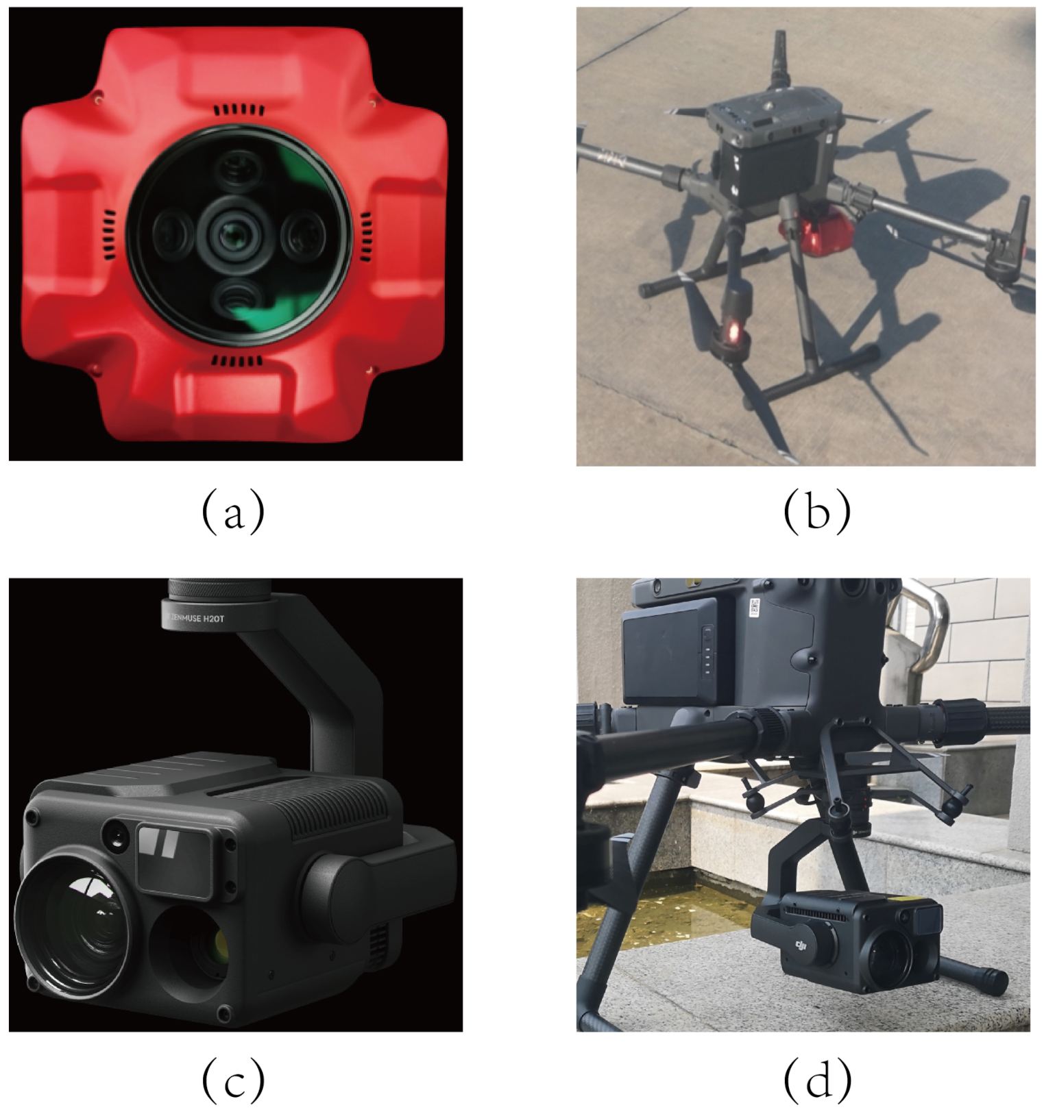
In Step 1 (showm in Figure 2), considering the effectiveness and efficiency, we first conducted day-time image acquisition with a five-eye tilt camera on a flight platform, with SHARE PSDK 102S (https://www.shareuavtec.com/ProductDetail/6519312.html, accessed on 1 October 2022) (shown in Figure 3a) and DJI M300 RTK (https://www.dji.com/cn/matrice-300?site=brandsite&from=nav, accessed on 1 October 2022) (shown in Figure 3b). The special SHARE 102S camera was composed of one vertical downward-facing lens and four 45-degree tilt lenses. Five overlapping images were recorded simultaneously for each shot as presented in Figure 4. For each single lens, more than 24 million pixels can be perceived. Furthermore, in order to fully and evenly cover the survey area, all flight paths were pre-planned in a grid fashion and automated by the flight control system supported by DJI M300. The images captured during this process were mainly used to reconstruct a high-precision 3D model. Sample images taken by PSDK 102S are shown in Figure 4.

Secondly, regarding the DJI H20T (https://www.dji.com/cn/zenmuse-h20-series?site=brandsite&from=nav, accessed on 1 October 2022) (as shown in Figure 3c) a visible light module was used to acquire another set of visible images, which have the same field of view as the corresponding thermal image. It acted as a "bridge" between thermal images and the reference 3D model, connecting the thermal image with other cross-view visible images and 3D point clouds. Similar to the previous operation, we mounted the H20T on the DJI M300 RTK, and captured the same scene again under well-lit conditions during the day. This time, in order to increase the diversity of data, we used two methods—planning route and free route—to collect images, and recorded the route information and the shooting angle of each image collection point.

Finally, we used the DJI H20T thermal module to obtain thermal images. The process was carried out with poor lighting conditions at night. It mainly used the track re-fly technique of the DJI M300 RTK to make the drone fly along the route where the bridge image is captured. During each trajectory, H20T captures the thermal images at the same angle and point as the bridge images thanks to the extremely small RTK error. As each thermal image has a corresponding bridge image, subsequent manual annotation earns facilitation. The image samples are shown in Figure 5.

In conclusion, our dataset contained three kinds of images in two modes, all of which hold their metadata, such as the focal length, aperture, and exposure. The specifications of the cameras used are shown in

Table 2. Cameras specifications.The specific parameters of the three cameras used in our dataset include resolution, wavelength range, and focal length.

Camera Model	Spectral Range (mm)	Image Size (pixels)	Focal Length (mm)	Equivalent Focal Length (mm)
SHARE PSDK 102S	0.4–0.7	6000 × 4000	35	35
DJI H20T Visible	0.4–0.7	5184 × 3888	6.83–119.94	31.7–556.2
DJI H20T Thermal	8–14	640 × 512	13.5	58

. At the same time, we recorded geo-referenced information (real-time kinematic positioning information) and flight control information (heading, speed, pitch, etc.) for the data acquisition process via the UAV platform.

3.2. Three-Dimensional Model Reconstruction

After obtaining the original data, we used the open-source system COLMAP [7] to reconstruct a 3D model from all visible images, as shown in Step 2 of Figure 2. The reconstructed point cloud is shown in Figure 6. Specifically, for each scene, the input resources included visible light images collected by the five-eye camera and the bridge images provided by H20T Visible during the day-time. The main pipeline of COLMAP [7] consists of feature extraction, image retrieval, structure-from-motion (SfM) and multi-view stereo (MVS).

Three files were output after the whole process: Cameras, Images, and Points3D. Camera records the intrinsic of each set of cameras. The format is as follows:

$$[Camera\_id,Model,Width,Height,Focal\_length,Cx,Cy]$$

where Model represents the camera model, which is all PINHOLE in our dataset, and $Cx$$Cy$ denotes the coordinate of the principal point. It should be noted that only the intrinsic parameters of visible light images are included, whereas the intrinsic parameters of thermal images are provided by DJI through camera calibration.

The Images contains the pose and feature points of each image. The specific form is as follows:

$$\begin{gathered} [Image\_id,(QWQXQYQZ),(TXTYTZ),Camera\_id,Name,Points2D] \\ Points2D:[Point2D\_id,X,Y,Point3D\_id] \end{gathered}$$

where $\left(QWQXQYQZ\right)$ represents the orientation in the form of quaternions, and $\left(TXTYTZ\right)$ represents the translation. The pose composed of them is the absolute pose in the 3D reference model. The one that needs to be detailed is Points2D. It contains the index and 2D coordinates of all of the 2D feature points in the image, as well as the 3D point id for each point. If the $point3D\_id$ is −1, it means that the point is not visible in the point cloud and is a point that failed to triangulate.

The Points3D is the 3D point cloud of the scene, representing the spatial structure of the entire scene. It stores the id, coordinates, color, and track of each 3D point as follows:

$$\begin{gathered} [Point3D\_id,(XYZ),(RGB),Track] \\ Track:[Image\_id,Point2D\_id] \end{gathered}$$

Each track contains multiple $[image\_id,Point2Did]$. This represents the image with $Image\_id$ that can observe this 3D point, and the index of the corresponding 2D feature point on this image.

Although COLMAP [7] does not have the ability to register thermal images to the 3D reconstruction because of its disparate modality, bridge images can lend a help. This is owed to bridge images having the same visual field as the corresponding thermal images, and the 3D points observed by the bridge image can also be observed by the thermal one. With this premise, we can easily establish the 2D-3D structure correspondences between the thermal image and the pre-built point cloud.

3.3. Semi-Automatic Supervision Generation

In the first two steps, we obtained all raw images and reference 3D models, after which, we performed semi-automatic supervision generation. Essentially, the thermal image was annotated to obtain its absolute pose. To obtain the absolute pose of the thermal image, we first needed to establish a one-to-one correspondence between the 2D points of the thermal image and the 3D points in the reference model. Since thermal images are not involved in the reconstruction process of 3D models, we accomplished this goal with the help of bridge images. Specifically, as shown in Step 3 of Figure 2, we first retrieved the bridge image from Images (generated in Section 3.2) based on the image name, and then we read all $Points2D$ data of this bridge image and selected all of the points whose $Point3D\_id$ was not −1; that is, those points with visibility. Finally, we marked the bridge image with a pink cross at these coordinates (X, Y) of those visible points, as shown in Figure 7a.

Next, we selected the markers that are easy for humans to recognize, such as the edge point of objects and corner points of buildings. We marked the center of the pink cross in Hugin (https://github.com/ndevenish/Hugin, accessed on 10 October 2022) as accurately as possible, and recorded the coordinate of this point, denoted by $(X_{select},Y_{select})$. Meanwhile, we marked one point with the closest appearance in the thermal image, and recorded the coordinate $(x,y)$. We simply used Hugin to mark tie points between thermal–visible image pairs and recorded the coordinates of manually labeled points.

Another key step is to find the 3D point corresponding to this pair of manual tie points. In the bridge image, we found the closest pixel distance to $(X_{select},Y_{select})$ from the cross-marked points. According to the previous description, the cross mark denotes a 2D feature point, which corresponds to a $Point3D\_id$ in the 3D point cloud. Then, we obtained the coordinates $(X,Y,Z)$ of this 3D point by id in Points3D (generated in Section 3.2). Through this labeling process, we matched the 3D point $(X,Y,Z)$ with the 2D point $(x,y)$ labeled on the thermal image. To ensure that the final pose could be computed successfully, we matched 15 to 30 points manually for each set of bridge–thermal images. The total number of annotated image pairs reached 898.

Finally, given the intrinsic parameters of the thermal camera and the 2D-3D matching, we could use the PnP solver [38,39] to compute the absolute pose of the thermal image as $Pos{e}_T$.

In the above step, we only manually matched 898 bridge–thermal image pairs to obtain the pose of the thermal images. In order to generate a large amount of supervision for multi-view visible–thermal image pairs to effectively train the model based on learning, we needed to propagate the annotation information to all visible images through the bridge image, so as to realize efficient semi-automatic supervision generation.

The premise of all of this is that the associated multi-view visible image of each bridge image was acquired in 3D model reconstruction (Section 3.2 and Step 2 shown in Figure 2) Because SfM and MVS ensure that these multi-view visible images share part of the track and have a sufficient overlap with the bridge images, for each bridge image, there are tens or even hundreds of associated images, as shown in Figure 8a.

The key to our efficient semi-automatic supervision generation method, and the reason why we collect bridge images, is to make the thermal image have the same field of view as the bridge image. In this way, the images associated with the bridge image are guaranteed to have a sufficient overlap with the thermal image. In other words, those multi-view images related to the thermal image can be retrieved in the whole image gallery by the bridge image, as shown in Figure 8b.

After obtaining the above retrieval relationship between thermal and visible images, we can semi-automatically generate supervision from their pose, intrinsic parameters, and depth. Here, pose represents the absolute pose of each image in the scene, which is denoted by T, as shown in Equation (1).

$$T=\left[\begin{array}{cc}R& t\\ {\mathbf{0}}^T& 1\end{array}\right]$$

(1)

The R, t stand for the rotation matrix and translation, respectively. The intrinsic parameter can generally be represented by the matrix in Equation (2), where f is the focal length and $c_x$ and $c_y$ constitute the coordinate of the principal point. It should be noted that the camera model used in the whole process is PINHOLE.

$$K=\left[\begin{array}{ccc}f& 0& c_x\\ 0& f& c_y\\ 0& 0& 1\end{array}\right]$$

(2)

Assuming that we have obtained poses of two thermal and visible images in the previous step as $T_T$ and $T_V$, as shown in Equation (3), given the depth map of the visible image, which stores the depth value for each pixel coordinate $(u,v)$, we aim to build dense correspondences.

$$T_V=\left[\begin{array}{cc}{R}_V& t_V\\ {\mathbf{0}}^T& 1\end{array}\right],T_T=\left[\begin{array}{cc}{R}_T& t_T\\ {\mathbf{0}}^T& 1\end{array}\right]$$

(3)

Figure 9 illuminates the basic matching process, where the subscripts V and T represent the visible and thermal image, respectively. Based on the PINHOLE projection function Equation (4), we built the relationship between the 3D point $P={(X_W,Y_W,Z_W,1)}^T$ (world coords) and 2D pixel $P={(u,v,1)}^T$ (pixel coords).

$$Z_{Cam}\left[\begin{array}{c}u\\ v\\ 1\end{array}\right]=\left[\begin{array}{cccc}f& 0& c_x& 0\\ 0& f& c_y& 0\\ 0& 0& 1& 0\end{array}\right]\left[\begin{array}{cc}R& t\\ {\mathbf{0}}^T& 1\end{array}\right]\left[\begin{array}{c}{X}_W\\ Y_W\\ Z_W\\ 1\end{array}\right]=\left[K\right|0]T\left[\begin{array}{c}{X}_W\\ Y_W\\ Z_W\\ 1\end{array}\right]$$

(4)

For a certain point $p_V={(u_V,v_V,1)}^T$ in the visible image, where $Z_V$ is the depth value of the point, we obtained its corresponding 3D point by modified projection Equation (5), where one transformation from nonhomogeneous to homogeneous coordinates is implied, since the result of the last three terms operation is nonhomogeneous.

$$\left[\begin{array}{c}{X}_W\\ Y_W\\ Z_W\\ 1\end{array}\right]=T_V^{-1}(K_V^{-1}{Z}_V\left[\begin{array}{c}{u}_V\\ v_V\\ 1\end{array}\right])$$

(5)

We then transformed it to the camera coordinate system of the thermal image by $T_T$ Equation (6). The P point was then projected to the imaging plane by the intrinsic parameter Equation (7). Finally, by eliminating $Z_T$, we could obtain the pixel coordinates of the corresponding points in the thermal image homogeneously.

$$\left[\begin{array}{c}{X}_T\\ Y_T\\ Z_T\\ 1\end{array}\right]=\left[\begin{array}{cc}{R}_T& t_T\\ {\mathbf{0}}^T& 1\end{array}\right]\left[\begin{array}{c}{X}_W\\ Y_W\\ Z_W\\ 1\end{array}\right]$$

(6)

$$Z_T\left[\begin{array}{c}{u}_T\\ v_T\\ 1\end{array}\right]=\left[\begin{array}{c}{f}_T{X}_T+c_x{Z}_T\\ f_T{Y}_T+c_y{Z}_T\\ Z_T\end{array}\right]=\left[\begin{array}{cccc}{f}_T& 0& c_x& 0\\ 0& f_T& c_y& 0\\ 0& 0& 1& 0\end{array}\right]\left[\begin{array}{c}{X}_T\\ Y_T\\ Z_T\\ 1\end{array}\right]$$

(7)

In summary, we obtained the point-to-point correspondence between visible $(u_V,v_V)$ and thermal $(u_T,v_T)$ by Equation (8).

$$Z_T\left[\begin{array}{c}{u}_T\\ v_T\\ 1\end{array}\right]=\left[K_T\right|0]T_T{T}_V^{-1}{K}_V^{-1}{Z}_V\left[\begin{array}{c}{u}_V\\ v_V\\ 1\end{array}\right]$$

(8)

Therefore, tens or even hundreds of multi-view thermal–visible image pairs with pixel-wise correspondence can be obtained simply by manually labeling a pair of bridge–thermal images. As a result, our method achieved the goal of efficiently generating a large number of multi-view and cross-spectral image matching supervision in a semi-automatic manner.

4. Experiment

In this part, we first introduce the implementation details of our experiment (Section 4.1), including the flight parameters during data collection, the way to divide the data set, and the software and hardware configuration of the experimental platform. We then evaluated the accuracy of our dataset by the re-projection error of the manual tie points, and explained in detail how the error of R, t was calculated for the experiments afterwards (Section 4.2). To verify the effectiveness of our dataset, we chose several representative image matching and re-localization methods discussed in Section 2.3 as solid baselines to test our MTV dataset. These baselines include traditional methods and learning-based methods, and we performed a relative pose estimation and absolute pose estimation to compare these methods. In the experiment of the relative pose (Section 4.3), we divided the selected methods into local feature-free and local feature-based to compare the differences between them. In the experiment of absolute pose, we divided it into matching-based methods and end-to-end methods (Section 4.4).

4.1. Implementation Details

Flight settings. To ensure the efficiency and accuracy of the collection, when using the five-eye camera, we set the flight height to 120 m, the course overlap rate and the side overlap rate to both 80%, and the flight speed to 10 m/s and, when we employed the thermal camera, we controlled the flight speed to 5–10 m/s and the flight altitude to 90–130 m.

Distribution and partitioning of the dataset. We collected data in five completely different scenarios, covering urban, rural, competition venues, etc. They have completely different types of texture information: not only areas with distinct contour lines, but also areas with weak textures and repeated textures. This makes our dataset diverse enough to provide a better generalization for algorithms trained on it. The specific data statistics are shown in

Table 3. Number of various images.

Scene	Image Type	Number of Images
race track	database visible	476
	bridge visible	60
	query thermal	60
building	database visible	1850
	bridge visible	341
	bridge thermal	341
countryroad	database visible	1018
	bridge visible	101
	query thermal	101
park	database visible	950
	bridge visible	234
	query thermal	234
villa	database visible	837
	bridge visible	162
	query thermal	162
total	database visible	5131
	bridge visible	898
	query thermal	898

.

We divided the thermal images into three groups: 80% for training, 10% for validation, and 10% for testing, and relative pose pairs were generated by them. Details are shown in

Table 4. We divided the data into three parts according to the ratio of 8:1:1, namely training, validation, and test sets.

Set	Number of Thermal Images	Number of Pairs
train	716	33,138
validation	89	3476
test	93	4050

.

Experimental settings. All of the learning-based methods in this section, including LoFTR [33], QuadTreeAttention [34], D2-Net [32], and PixLoc [37], were trained and tested on our dataset using the same partitioning rules. However, SIFT [1] does not require training, so only the test set was used. Our main experimental platform was a workstation with two RTX 3090s. For all experiments, the initial learning rate was set to 0.008, and the training duration was up to 300 epoch. All models were trained end-to-end with randomly initialized weights.

4.2. Evaluation and Metric

Evaluation. To estimate the accuracy of all manual tie points as well as the subsequent solved poses, we measured the re-projection error of these manual tie points on the registered thermal images. We projected the selected 3D points onto the thermal image through the pose $T_T$ of the thermal image to obtain the coordinate $(x^{\prime },y^{\prime })$ of projection points. Then, we calculated the pixel error between $(x^{\prime },y^{\prime })$ and the manual tie point coordinate $(x,y)$. This is visualized in Figure 10.

The results of the quantization are shown in the following

Table 5. Re-projection error(px) of manual tie points.

Scene	Maximum	Standard Deviation	Average
race track	3.67	1.08	1.47
building	3.24	1.11	1.36
countryroad	4.41	1.87	1.97
park	5.93	1.76	1.72
villa	4.05	1.32	1.48
total	5.93	1.56	1.55

. The average re-projection error is $1.55$ pixels for the registered thermal image of $640\times 512$ resolution, which is fully sufficient for the training and testing of deep-learning-based matching algorithms.

In addition, our visualization of mapping pixels on the visible image of non-bridges to thermal is shown in Figure 11, which can be seen to have very dense pixel-wise correspondences.

Metric. In this section, we describe how the error between the estimate and the true value is calculated for the relative pose and absolute pose experiments. In the relative pose experiment, because there is no absolute translation, we could only calculate the angle between the two translation vectors in space to evaluate the translation error, as shown in Equation (9). In the absolute pose, the position error $|t_{err}|$ is the Euclidean distance between the estimated position and the true position, and can be computed with Equation (10).

$$t_{err}=arccos(\frac{t_{est}·t_{gt}}{|t_{est}\left|\right|t_{est}|})$$

(9)

$$t_{err}=|t_{gt}-t_{est}|$$

(10)

The orientation error $|R_{err}|$ is measured in Euler angle and calculated from the estimated ($R_{est}$) and true ($R_{gt}$) camera rotation matrices. This is the standard used to calculate the rotation angle [40]. Therefore, the Euler angle error can be used by Equation (11).

$$R_{err}=|arccos(\frac{trace(R_{est}^T·R_{gt})-1}{2})|$$

(11)

4.3. Relative Pose

Evaluation protocol. We evaluated the matching results using the AUC of the pose error at thresholds (5°, 10°, 20°), where the pose error is defined as the larger one of the angular error of rotation and translation. To recover the camera pose, we used RANSAC to solve the essential matrix that predicts the match.

Methods. Local feature-free methods such as LoFTR [33] and QuadTreeAttention [34] will directly generate matching results, whereas SIFT [1] and D2-Net [32] extract feature points and descriptors. Thus, they need the nearest neighbors to match the descriptors. Finally, the relative pose was calculated using the eight-point method by matching points, and the error was calculated from the true value.

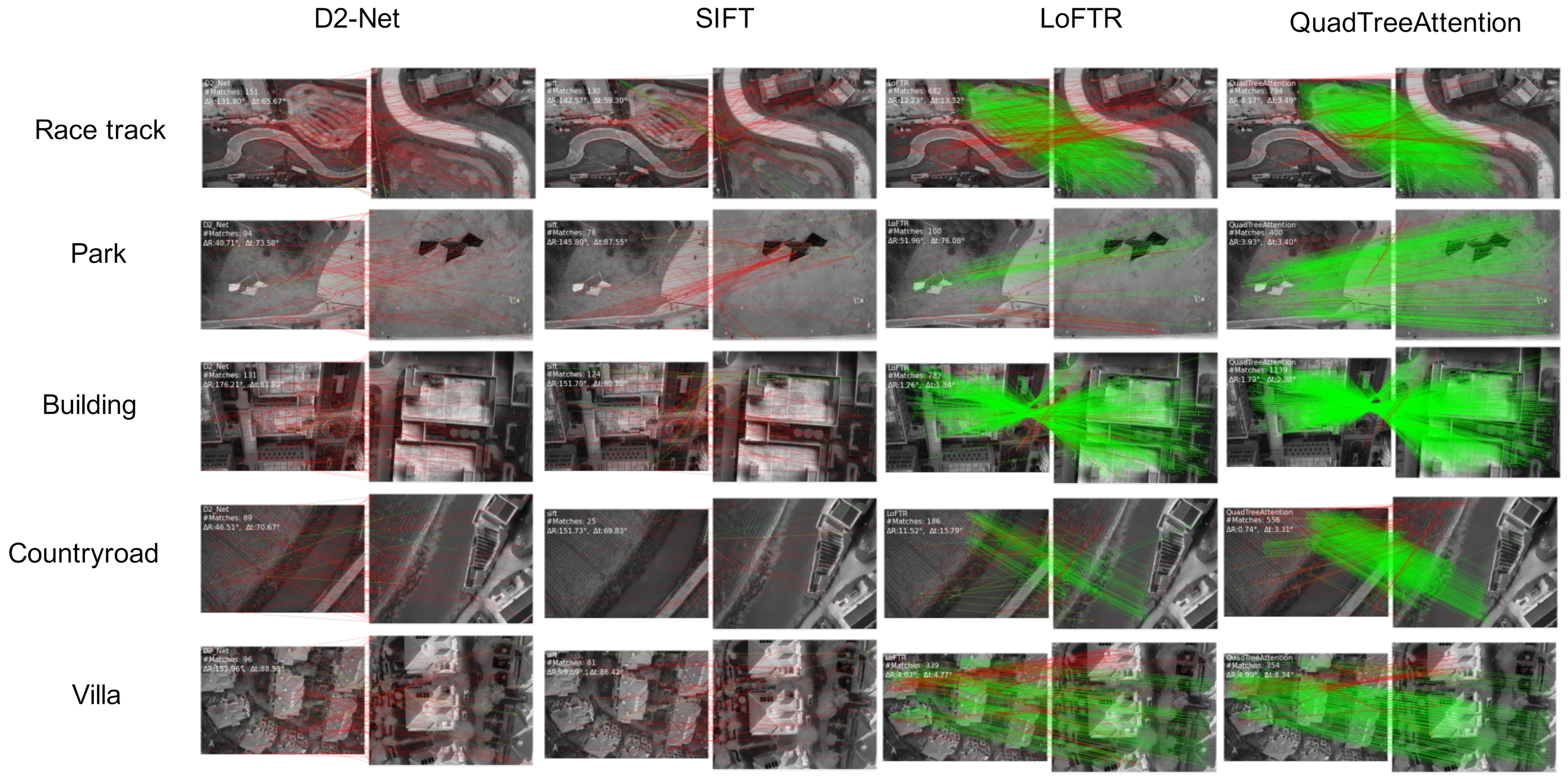
Results. An error comparison is shown in the following

Table 6. Evaluation on test set for relative pose estimation.

Category	Methods	Precision	Pose Estimation AUC
			@5°	@10°	@20°
local feature-free	LoFTR	0.6681	6.9995	15.9352	27.4986
	QuadTreeAttention	0.7897	10.2474	21.7289	34.5145
local feature-based	D2-Net + NN	0.1617	0	0	0
	SIFT + NN	0.1450	0	0	0

. It is clear that QuadTreeAttention can achieve a better performance. However, the AUC of all methods is at a low level. More matching visualization and qualitative results can be found in Figure 12.

4.4. Absolute Pose

Evaluation protocol. We reported the median translation (cm) and rotation (degree) errors and localization recall at thresholds (25 cm, 2°), (50 cm, 5°), and (500 cm, 10°).

Methods. Besides the relative pose estimation, our dataset can also validate low-light visual localization, where the task is to estimate the 6-DoF poses of given thermal images with the reference 3D scene model. We added the end-to-end method pixloc [37] for comparison in the absolute pose experiments. The image matching-based method above calculates the absolute poses by feeding the 2D-2D matching results into Hloc [41,42].

Results. A comparison of median translation and rotation errors is shown in the

Table 7. We report the median translation (cm) and rotation (°) errors. LoFTR achieves the smallest median translation error in three scenarios and the smallest median rotation in two scenarios. The best one is shown in bold font.

Category	Methods	Median Translation (cm) and Rotation (°) Errors
		Villa	Park	Countryroad	Building	Race Track
Matching-based	LoFTR+Hloc	4.893 /0.569	18.447/2.820	17.441/1.369	4.004/0.803	16.835/1.613
	QuadTreeAttention+Hloc	6.504/0.743	22.144/3.356	18.958/1.595	4.372/0.885	13.927/1.310
	D2-Net+NN+Hloc	561.709/132.139	448.046/122.489	801.142/122.861	323.107/127.448	614.754/109.771
	SIFT+NN+Hloc	734.868/113.349	1075.445/103.022	1844.120/109.922	745.144/108.854	73.666/7.121
End-to-End	PixLoc	12.949/0.947	19.393/2.132	10.568/2.251	17.619/2.255	23.980/1.361

, whereas localization recall is shown in the

Table 8. We report the localization recall at thresholds (25 cm, 2°), (50 cm, 5°), and (500 cm, 10°). The best results are in bold.

Category	Methods	Localization Recall at Thresholds (25 cm, 2°), (50 cm, 5°), and (500 cm, 10°)
		Villa	Park	Countryroad	Building	Race Track
Matching-based	LoFTR+Hloc	82.35/88.24/94.12	29.17/75.00/95.83	72.73/90.91/100.00	88.57/97.14/97.14	66.67/100.00/100.00
	QuadTreeAttention+Hloc	88.24/88.24/94.12	41.67/87.50/95.83	63.64/100.00/100.00	88.57/91.43/97.14	66.67/100.00/100.00
	D2-Net+NN+Hloc	0/0/0	0/4.17/4.17	0/0/0	0/0/0	0/0/0
	SIFT+NN+Hloc	0/0/0	4.17/16.67/20.83	0/0/0	0/0/0	0/50.00/50.00
End-to-End	PixLoc	76.47/88.24/94.12	45.83/87.50/95.83	45.45/63.64/100.00	31.43/65.71/94.29	50.00/100.00/100.00

. Overall, QuadTreeAttention+Hloc achieves better results.

5. Discussion

Analysis. As shown in Figure 12, from the visualized matching results, we observe that, for cross-spectral image matching, SIFT [1], D2-Net [32], and other methods that independently extract image features and then match descriptors nearly fail to successfully match. Most of the feature points extracted by them are based on pixel gradients, corner points, textures, etc. However, they fail to adequately extract features and generate effective descriptors for thermal images with weak textures or large regions of repeated textures. Therefore, pairs of images cannot be correlated. Local feature-free matching methods such as LoFTR [33] and QuadTreeAttention [34] achieve a relatively decent performance. This is because they use a multi-scale receptive field to extract deep features from the image and give uniqueness to all points in the image via position encoding and the transformer structure. Thus, those regions of weak and repeated textures can also be matched efficiently. This is also demonstrated by the quantitative measure of the relative pose, as shown in Table 6. Regarding both the accuracy of the matching and the AUC of the pose under the three thresholds, the local feature-free method significantly outperforms the local feature-based method. However, in general, both learning-based and feature-based methods suffer from a large number of spurious matches, indicating that there is still considerable room for improvement in the matching performance. For the absolute pose estimation, as shown in Table 7 and Table 8, the local feature-free matching method outperforms the end-to-end method and significantly outperforms the detector-based method. This result is roughly the same as in the visible image matching case. Therefore, the future development of matching methods between visible images will also contribute to thermal visible matching.

Limitations. While the semi-automatic supervision generation in the proposed dataset construction method can efficiently generate a large number of paired images across viewpoints, it has some limitations. To obtain bridge images, which play a key role in the data annotation process, we need to use UAVs with high-precision localization capabilities and track records. As a result, there are certain restrictions on the selection of acquisition equipment. In addition, oblique photography cameras for large-scale, high-precision modeling are also relatively more expensive than regular cameras. However, for small-scale scenarios, our method can also be applied to more easily accessible devices.

6. Conclusions

The main contribution of this paper is the construction of a multi-view thermal and visible aerial image dataset consisting of multiple scenes. We described in detail the method of data acquisition and the parameters of the devices used. Overall, the dataset includes visible and thermal images, metadata with geo-reference, and 3D models based on visible images. In addition, 898 thermal images were manually matched with feature points from visible images taken at the same pose. In contrast to previous datasets, we mainly provide high-precision 3D reference models, resulting in thermal image poses with much smaller errors. Our semi-automatic method for generating supervision, with human guidance, can efficiently obtain a large number of supervision signals for pixel-wise matching between cross-view cross-spectral image pairs. Therefore, our dataset can be used for the training of learning-based methods. Moreover, the 6-DoF pose between thermal and visible images in the dataset is crucial for the localization task. Thus, this dataset can not only be used to study thermal–visible image matching, but also to study the localization of thermal images. It provides the possibility of visual localization for UAV with a thermal sensor under low-illumination conditions. Further work could also apply this dataset to retrieval between thermal and visible images.

References

1. Lowe, D.G. Object recognition from local scale-invariant features. In Proceedings of the Seventh IEEE International Conference on Computer Vision, Corfu, Greece, 20–25 September 1999; IEEE: Piscataway, NJ, USA, 1999; Volume 2, pp. 1150–1157. [Google Scholar]
2. Li, Z.; Snavely, N. Megadepth: Learning single-view depth prediction from internet photos. In Proceedings of the IEEE Conference on Computer Vision and Pattern Recognition, Salt Lake City, UT, USA, 18–23 June 2018; pp. 2041–2050. [Google Scholar]
3. Dai, A.; Chang, A.X.; Savva, M.; Halber, M.; Funkhouser, T.; Nießner, M. Scannet: Richly-annotated 3d reconstructions of indoor scenes. In Proceedings of the IEEE Conference on Computer Vision and Pattern Recognition, Honolulu, HI, USA, 21–26 July 2017; pp. 5828–5839. [Google Scholar]
4. Zhang, X.; Ye, P.; Xiao, G. VIFB: A visible and infrared image fusion benchmark. In Proceedings of the IEEE/CVF Conference on Computer Vision and Pattern Recognition Workshops, Seattle, WA, USA, 14–19 June 2020; pp. 104–105. [Google Scholar]
5. Toet, A. The TNO multiband image data collection. Data Brief 2017, 15, 249. [Google Scholar] [CrossRef] [PubMed]
6. Jia, X.; Zhu, C.; Li, M.; Tang, W.; Zhou, W. LLVIP: A Visible-infrared Paired Dataset for Low-light Vision. In Proceedings of the IEEE/CVF International Conference on Computer Vision, Montreal, QC, Canada, 10–17 October 2021; pp. 3496–3504. [Google Scholar]
7. Schonberger, J.L.; Frahm, J.M. Structure-from-motion revisited. In Proceedings of the IEEE Conference on Computer Vision and Pattern Recognition, Las Vegas, NV, USA, 27–30 June 2016; pp. 4104–4113. [Google Scholar]
8. Davis, J.W.; Sharma, V. Background-subtraction using contour-based fusion of thermal and visible imagery. Comput. Vis. Image Underst. 2007, 106, 162–182. [Google Scholar] [CrossRef]
9. Ellmauthaler, A.; Pagliari, C.L.; da Silva, E.A.; Gois, J.N.; Neves, S.R. A visible-light and infrared video database for performance evaluation of video/image fusion methods. Multidimens. Syst. Signal Process. 2019, 30, 119–143. [Google Scholar] [CrossRef]
10. INO. Available online: https://www.ino.ca/en/technologies/video-analytics-dataset/ (accessed on 17 October 2022).
11. Aguilera, C.A.; Sappa, A.D.; Toledo, R. LGHD: A feature descriptor for matching across non-linear intensity variations. In Proceedings of the 2015 IEEE International Conference on Image Processing (ICIP), Quebec City, QC, Canada, 27–30 September 2015; IEEE: Piscataway, NJ, USA, 2015; pp. 178–181. [Google Scholar]
12. Campo, F.B.; Ruiz, F.L.; Sappa, A.D. Multimodal stereo vision system: 3D data extraction and algorithm evaluation. IEEE J. Sel. Top. Signal Process. 2012, 6, 437–446. [Google Scholar] [CrossRef]
13. Barrera, F.; Lumbreras, F.; Sappa, A.D. Multispectral piecewise planar stereo using Manhattan-world assumption. Pattern Recognit. Lett. 2013, 34, 52–61. [Google Scholar] [CrossRef]
14. Aguilera, C.; Barrera, F.; Lumbreras, F.; Sappa, A.D.; Toledo, R. Multispectral image feature points. Sensors 2012, 12, 12661–12672. [Google Scholar] [CrossRef] [Green Version]
15. Fu, Z.; Qin, Q.; Luo, B.; Wu, C.; Sun, H. A local feature descriptor based on combination of structure and texture information for multispectral image matching. IEEE Geosci. Remote Sens. Lett. 2018, 16, 100–104. [Google Scholar] [CrossRef]
16. Fu, Z.; Qin, Q.; Luo, B.; Sun, H.; Wu, C. HOMPC: A local feature descriptor based on the combination of magnitude and phase congruency information for multi-sensor remote sensing images. Remote Sens. 2018, 10, 1234. [Google Scholar] [CrossRef] [Green Version]
17. García-Moreno, L.M.; Díaz-Paz, J.P.; Loaiza-Correa, H.; Restrepo-Girón, A.D. Dataset of thermal and visible aerial images for multi-modal and multi-spectral image registration and fusion. Data Brief 2020, 29, 105326. [Google Scholar] [CrossRef] [PubMed]
18. Chen, D.M.; Baatz, G.; Köser, K.; Tsai, S.S.; Vedantham, R.; Pylvänäinen, T.; Roimela, K.; Chen, X.; Bach, J.; Pollefeys, M.; et al. City-scale landmark identification on mobile devices. In Proceedings of the 24th IEEE Conference on Computer Vision and Pattern Recognition CVPR 2011, Colorado Springs, CO, USA, 20–25 June 2011; IEEE: Piscataway, NJ, USA, 2011; pp. 737–744. [Google Scholar]
19. Irschara, A.; Zach, C.; Frahm, J.M.; Bischof, H. From structure-from-motion point clouds to fast location recognition. In Proceedings of the 2009 IEEE Conference on Computer Vision and Pattern Recognition, Miami, FL, USA, 20–25 June 2009; IEEE: Piscataway, NJ, USA, 2009; pp. 2599–2606. [Google Scholar]
20. Sattler, T.; Torii, A.; Sivic, J.; Pollefeys, M.; Taira, H.; Okutomi, M.; Pajdla, T. Are large-scale 3d models really necessary for accurate visual localization? In Proceedings of the IEEE Conference on Computer Vision and Pattern Recognition, Honolulu, HI, USA, 21–26 July 2017; pp. 1637–1646. [Google Scholar]
21. Carlevaris-Bianco, N.; Ushani, A.K.; Eustice, R.M. University of Michigan North Campus long-term vision and lidar dataset. Int. J. Robot. Res. 2016, 35, 1023–1035. [Google Scholar] [CrossRef]
22. Sattler, T.; Maddern, W.; Toft, C.; Torii, A.; Hammarstrand, L.; Stenborg, E.; Safari, D.; Okutomi, M.; Pollefeys, M.; Sivic, J.; et al. Benchmarking 6dof outdoor visual localization in changing conditions. In Proceedings of the IEEE Conference on Computer Vision and Pattern Recognition, Salt Lake City, UT, USA, 18–23 June 2018; pp. 8601–8610. [Google Scholar]
23. Firmenichy, D.; Brown, M.; Süsstrunk, S. Multispectral interest points for RGB-NIR image registration. In Proceedings of the 2011 18th IEEE International Conference on Image Processing, Brussels, Belgium, 11–14 September 2011; IEEE: Piscataway, NJ, USA, 2011; pp. 181–184. [Google Scholar]
24. Maddern, W.; Vidas, S. Towards robust night and day place recognition using visible and thermal imaging. In RSS 2012 Workshop: Beyond Laser and Vision: Alternative Sensing Techniques for Robotic Perception; University of Sydney: Sydney, Australia, 2012; pp. 1–6. [Google Scholar]
25. Ricaurte, P.; Chilán, C.; Aguilera-Carrasco, C.A.; Vintimilla, B.X.; Sappa, A.D. Feature point descriptors: Infrared and visible spectra. Sensors 2014, 14, 3690–3701. [Google Scholar] [CrossRef] [PubMed] [Green Version]
26. Sappa, A.D.; Carvajal, J.A.; Aguilera, C.A.; Oliveira, M.; Romero, D.; Vintimilla, B.X. Wavelet-based visible and infrared image fusion: A comparative study. Sensors 2016, 16, 861. [Google Scholar] [CrossRef] [PubMed] [Green Version]
27. Johansson, J.; Solli, M.; Maki, A. An evaluation of local feature detectors and descriptors for infrared images. In Proceedings of the European Conference on Computer Vision, Amsterdam, The Netherlands, 11–14 October 2016; Springer: Berlin/Heidelberg, Germany, 2016; pp. 711–723. [Google Scholar]
28. Bonardi, F.; Ainouz, S.; Boutteau, R.; Dupuis, Y.; Savatier, X.; Vasseur, P. PHROG: A multimodal feature for place recognition. Sensors 2017, 17, 1167. [Google Scholar] [CrossRef] [PubMed] [Green Version]
29. Vidas, S.; Sridharan, S. Hand-held monocular slam in thermal-infrared. In Proceedings of the 2012 12th International Conference on Control Automation Robotics & Vision (ICARCV), Guangzhou, China, 5–7 December 2012; IEEE: Piscataway, NJ, USA, 2012; pp. 859–864. [Google Scholar]
30. Maddern, W.; Stewart, A.; McManus, C.; Upcroft, B.; Churchill, W.; Newman, P. Illumination invariant imaging: Applications in robust vision-based localisation, mapping and classification for autonomous vehicles. In Proceedings of the Visual Place Recognition in Changing Environments Workshop, IEEE International Conference on Robotics and Automation (ICRA), Hong Kong, China, 31 May–5 June 2014; Volume 2, p. 5. [Google Scholar]
31. Borges, P.V.K.; Vidas, S. Practical infrared visual odometry. IEEE Trans. Intell. Transp. Syst. 2016, 17, 2205–2213. [Google Scholar] [CrossRef]
32. Dusmanu, M.; Rocco, I.; Pajdla, T.; Pollefeys, M.; Sivic, J.; Torii, A.; Sattler, T. D2-net: A trainable cnn for joint description and detection of local features. In Proceedings of the IEEE/CVF Conference on Computer Vision and Pattern Recognition, Long Beach, CA, USA, 15–20 June 2019; pp. 8092–8101. [Google Scholar]
33. Sun, J.; Shen, Z.; Wang, Y.; Bao, H.; Zhou, X. LoFTR: Detector-free local feature matching with transformers. In Proceedings of the IEEE/CVF Conference on Computer Vision and Pattern Recognition, Nashville, TN, USA, 20–25 June 2021; pp. 8922–8931. [Google Scholar]
34. Tang, S.; Zhang, J.; Zhu, S.; Tan, P. QuadTree Attention for Vision Transformers. arXiv 2022, arXiv:2201.02767. [Google Scholar]
35. Aguilera, C.A.; Aguilera, F.J.; Sappa, A.D.; Aguilera, C.; Toledo, R. Learning cross-spectral similarity measures with deep convolutional neural networks. In Proceedings of the IEEE Conference on Computer Vision and Pattern Recognition Workshops, Las Vegas, NV, USA, 26 June–1 July 2016; pp. 1–9. [Google Scholar]
36. Cui, S.; Ma, A.; Wan, Y.; Zhong, Y.; Luo, B.; Xu, M. Cross-modality image matching network with modality-invariant feature representation for airborne-ground thermal infrared and visible datasets. IEEE Trans. Geosci. Remote Sens. 2021, 60, 1–14. [Google Scholar] [CrossRef]
37. Sarlin, P.E.; Unagar, A.; Larsson, M.; Germain, H.; Toft, C.; Larsson, V.; Pollefeys, M.; Lepetit, V.; Hammarstrand, L.; Kahl, F.; et al. Back to the feature: Learning robust camera localization from pixels to pose. In Proceedings of the IEEE/CVF Conference on Computer Vision and Pattern Recognition, Nashville, TN, USA, 20–25 June 2021; pp. 3247–3257. [Google Scholar]
38. Mach, C.; Bolles, R.C. Random Sample Consensus: A paradigm for model fitting with application to image analysis and automated cartography. Readings Comput. Vis. 1981, 24, 726–740. [Google Scholar]
39. Kneip, L.; Scaramuzza, D.; Siegwart, R. A novel parametrization of the perspective-three-point problem for a direct computation of absolute camera position and orientation. In Proceedings of the 24th IEEE Conference on Computer Vision and Pattern Recognition CVPR 2011, Colorado Springs, CO, USA, 20–25 June 2011; IEEE: Piscataway, NJ, USA, 2011; pp. 2969–2976. [Google Scholar]
40. Hartley, R.; Trumpf, J.; Dai, Y.; Li, H. Rotation averaging. Int. J. Comput. Vis. 2013, 103, 267–305. [Google Scholar] [CrossRef]
41. Sarlin, P.E.; Cadena, C.; Siegwart, R.; Dymczyk, M. From Coarse to Fine: Robust Hierarchical Localization at Large Scale. In Proceedings of the IEEE/CVF Conference on Computer Vision and Pattern Recognition CVPR, Long Beach, CA, USA, 15–20 June 2019. [Google Scholar]
42. Sarlin, P.E.; DeTone, D.; Malisiewicz, T.; Rabinovich, A. SuperGlue: Learning Feature Matching with Graph Neural Networks. In Proceedings of the IEEE/CVF Conference on Computer Vision and Pattern Recognition CVPR, Seattle, WA, USA, 13–19 June 2020. [Google Scholar]
Figure 1. A sample of these two types of images. Compared to visible light photos at night, thermal images are imaged through temperature differences and can capture sharper edges and textures at night. (a) Visible daytime, (b) Visible night-time, (c) Thermal nighttime.
Remotesensing 15 00174 g001
Figure 2. Overview of the dataset construction. The construction of MTV has three components. Step 1: Data acquisition. We needed to collect different images three times. First, we used an oblique photography camera to take highly overlapping visible light images during the day. The route is shown as the S-track in green. This set of images helps us to reconstruct a high-quality reference 3D model. Then, also during the day, we performed multi-view aerial photography using the visible light lens of the H20T to acquire bridge images. During this time, the flight path and camera perspective were recorded. Finally, we used the H20T thermal lens, following the same flight path and settings as the bridge image, to take thermal images at night, as detailed in Section 3.1. Step 2: 3D model reconstruction. All of the visible images acquired in Step 1, including PSDK 102S and DJI H20T Visible, were imported into the offline reconstruction software Colmap [7] for SfM and MVS reconstruction. The output of this step is the absolute pose and depth map of all visible images, denoted by P o s e V and d e p t h V , as detailed in Section 3.2. Step3: Supervision generation. Firstly, according to the visibility, the 3D points of the reference model were projected onto the bridge image to generate marker points. Then, markers that are easy to recognize were picked, while the corresponding points of these markers were manually matched in the thermal image. In this way, we obtained a 2D-3D correspondence between the thermal image and the reference model. The absolute pose of the thermal image ( P o s e T ) was obtained using the PnP [38,39] algorithm. Finally, with the P o s e V and d e p t h V obtained in the previous step, we could establish the pixel-wise correspondence of the overlapping regions in the thermal–visible image pair through the projection transformation between 2D-3D points, as detailed in Section 3.3.
Remotesensing 15 00174 g002
Figure 3. (a) Five-eye camera PDSK 102S. (b) DJI M300 with PDSK 102s. (c) DJI H20T. (d) DJI M300 with H20T.
Remotesensing 15 00174 g003
Figure 4. Sample images taken by PSDK 102S. Five images can be seen that were shot at the same time, so larger scenes can be covered faster.
Remotesensing 15 00174 g004
Figure 5. Visible and thermal images are very close in pose and field of view. (a) Visible, (b) Thermal.
Remotesensing 15 00174 g005
Figure 6. The reconstruction result of one scene in the dataset, where the red markers represent the image shooting points.
Remotesensing 15 00174 g006
Figure 7. Manual annotation of the thermal images. (a) The markers on the bridge image. (b) Labeling the tie points between the bridge and the thermal image.
Remotesensing 15 00174 g007
Figure 8. (a) The bridge image associates tens or even hundreds of images in the reference model. (b) Thermal image connects with multi-view images through the bridge image.
Remotesensing 15 00174 g008
Figure 9. We find the 3D point corresponding to the 2D points in the visible image by depth. Depth refers to the distance from the optical center O V to the projection of point P on the z-axis (camera coordinate system of visible image), as shown by the solid green line. The corresponding point on thermal image is then found by projecting this 3D point onto it. In this way, we can establish a pixel-wise correspondence from visible to thermal.
Remotesensing 15 00174 g009
Figure 10. The different color lines reflect the relative magnitude of the re-projection error, with the reddest approximately approaching the maximum error and the bluer closer to the minimum error. Simple statistics of the error for this image are annotated in the top left.
Remotesensing 15 00174 g010
Figure 11. Here is a non-bridge and thermal image pair from different viewpoints: the top is the original image, and the bottom is the result of visualizing our generated supervision.
Remotesensing 15 00174 g011
Figure 12. Match results visualization. The green line represents a correct match whose biased estimate of reprojection error is less than the threshold of 5 × 10 4 . In contrast, the red line represents an incorrect match. D2-Net and SIFT had almost no correct matches. LoFTR completed many correct matches but also had a large number of incorrect matches.
Remotesensing 15 00174 g012