Article

Parcel-Level Mapping of Horticultural Crops in Mountain Areas Using Irregular Time Series and VHR Images Taking Qixia, China as An Example

1
National Engineering Research Center for Geomatics, Aerospace Information Research Institute, Chinese Academy of Sciences, Beijing 100101, China
2
College of Resources and Environment, University of Chinese Academy of Sciences, Beijing 100049, China
3
Xinjiang Institute of Ecology and Geography, Chinese Academy of Sciences, Beijing 900931, China
4
Hangzhou Hikvision Digital Technology Co., Ltd., Hangzhou 310013, China
*
Author to whom correspondence should be addressed.
Remote Sens. 2023, 15(1), 175; https://doi.org/10.3390/rs15010175
Submission received: 4 October 2022 / Revised: 20 December 2022 / Accepted: 22 December 2022 / Published: 28 December 2022

Abstract

:
Accurate and reliable horticultural crop classification results are an important part of agricultural management. At present, research on orchard classification based on optical images in complex mountain areas is vulnerable to the influence of cloudy weather, especially in the summer, which leads to a lack of key phenological characteristics. To solve this problem, a parcel-level orchard mapping experiment with an irregular time series was carried out in Qixia City, China. Firstly, the candidate parcels in the study area were extracted from VHR images with a spatial resolution of 0.55 m based on RCF and DABNet models. The F1 score and area-based intersection-over-union (IoU) of the parcel extraction results were calculated. When the boundary buffer radius was 1 m, the F1 score was 0.93. When the radius was 2 m, the F1 score was 0.96. The IoU was 0.872, which shows the effectiveness of the parcel extraction method. Then, based on Sentinel-2 data, the NDVI, EVI, and SAVI vegetation indexes were calculated to construct an irregular time series. A two-dimensional CNN model was used for classification. In order to verify the effectiveness of this method, the study also constructed regular time series for the study area and conducted classification experiments using the 2DCNN and LSTM as classifiers, respectively. Confusion matrices were constructed for the classification results, and the overall accuracy was calculated. The results show that the overall accuracy of the method based on irregular time series is 97.76%, with a kappa coefficient of 0.96, higher than the other experiments, which indicates that the classification method based on irregular time series is effective and can make full use of the fragmented spectral features. Finally, based on the candidate parcels and pixel-level classification results of the study area, the crop categories of the parcels were filled to achieve accurate parcel-level mapping of horticultural crops in complex mountain areas. This method can provide a theoretical reference for orchard crop mapping and serves the development of regional precision agriculture.

1. Introduction

Horticultural crops are one of the most important agricultural production types in the world [1]. According to the National Bureau of Statistics of China, by the end of 2020, China’s orchard planting area reached 1.23 billion hectares and the fruit output reached 2.87 billion tons [2]. Among all fruits, citrus and apples are planted the most frequently. China is one of the most important horticultural crop-growing areas in the world. Regarding apples, for example, the output of apples in China accounts for 54.07% of the world total, making it the largest apple-producing country in the world [3]. In China, many garden crops are grown on complex terrain, mainly on hillside terraces, plains, and loess hilly areas, at altitudes of 50–2500 m. In this case, the question of how to obtain the planting information of horticultural crops quickly and accurately is of great significance for crop yield estimation and planting structure adjustment. Traditional crop planting information is mainly obtained by manual field statistics, which are costly and difficult to update. The development of remote sensing technology provides advanced and convenient technical means to solve this problem [4].
There has been much research on crop classification and mapping using remote sensing technology [4], and the mapping results have been used in many fields, such as crop yield estimation and water resource protection [5,6,7]. The mainstream crop classification methods reflect the biomass changes during crop growth by constructing the temporal characteristics of crops based on satellite images. Phenological differences between different crops are the main basis for classification. Most related experiments obtain pixel-level classification results [4]. However, due to the limitations of the satellite image resolution, there will be mixed-pixel phenomena in pixel-level classification. Moreover, the classification results show a salt and pepper effect [8], which is inconsistent with the actual planting situation, and land cover classification based on the pixel level cannot obtain the land surface farmland parcel information.
In this case, with the development of high-resolution images, many studies have attempted to apply some algorithms in the field of computer remote sensing in order to achieve object-level mapping [9,10,11,12,13]. Compared with the pixel-based classification method, this method can extract more semantic information and obtain farm parcel products [14]. Object-oriented classification methods are gradually becoming widely used in the field of agriculture, and it has been proven by many scholars that they have better classification accuracy than pixel-level methods [15,16,17,18]. Compared with a crop distribution with lower resolution, it is obvious that complete agricultural parcels are more conducive to agricultural management. In the early stage, the extraction method for objects were mainly based on segmentation algorithms. Objects are geographic units with homogeneous features obtained by pixel clustering [19,20]. This type of object does not consider the social attributes of farmland parcels, which are very different from the actual parcel [20]. Many deep learning models have been used to extract farmland parcels, and good results have been achieved [14,21].
In the current crop classification research, machine learning or deep learning algorithms are mostly used as classifiers, such as RF, SVM, LSTM, etc. [5,6,17,22,23,24,25,26]. The time series characteristics of the parcels are used as the input of the classifier to obtain the category attributes of the farm parcels [14,27]. These classifiers generally require that the inputs of the model be regular sample data—that is, the input time series data are regular image sequences of constant length, which requires the number of high-quality satellite images in the research scope to reach a certain extent; otherwise, the classification accuracy will be seriously affected [21]. In fact, in some regions with poor climate conditions, many optical satellite images will be obscured by clouds. Additionally, when the study area is large, the time series length of pixels in different spatial positions is inconsistent. In order to solve this problem, most of the already existing research obtained the regular time series characteristics of crops by preprocessing images. However, during this process, the available optical data is deleted, which may cause the original available observation information to not be fully utilized, affecting the accuracy of crop classification. In order to solve this problem, some scholars consider classifying crops based on irregular time series to improve the utilization of fragmented optical images [28,29,30]. In recent studies, the 2DCNN model has been applied for the classification of irregular time series and has successfully achieved high-precision crop yield estimations [31,32]. Pengyu Hao et al. [33] constructed irregular time series, successfully extracted the regional crop distribution, and explored the potential of irregular time series in crop classification. Their results show that using irregular time series data to construct crop growth characteristics can better characterize crop growth patterns and that optical images with different scales can be efficiently used. However, most of these works are carried out at the pixel level, and there is a lack of research on parcel-level irregular sequence mapping for garden crops.
It is urgently necessary to carry out the accurate classification of horticultural crops based on irregular time series in complex imaging areas. This study proposes a method for the parcel-level mapping of orchards based on irregular time series, and the VHR and Sentinel-2 optical images are used. Firstly, the deep learning algorithms RCF and DABNet are used to extract candidate parcels from the VHR images. Then, the vegetation indexes are calculated for Sentinel-2 images, and the irregular time series are constructed. The one-dimensional time series data are transformed into a three-dimensional matrix, and a new feature image is constructed for each pixel. Here, 2DCNN is used to classify the 3D feature data, and the pixel-level classification results of crops are obtained. In this method, the optical data are fragmented when dividing the grid, so that the optical image information of the study area can be fully utilized. Moreover, the characteristics are recombined in the time dimension to construct a fine crop growth curve, which can improve the classification accuracy of crops compared with the classification method based on regular time series. Finally, based on the candidate parcels and pixel-level classification results, a filling strategy is designed. Differing from the method of feature construction and classification using parcels as the minimum unit, parcels are used as the spatial constraints of pixel-level classification results for parcel type filling to obtain regional parcel-level horticultural crop distribution mapping. The experiment was carried out in Qixia City, Shandong Province, China, and the distribution of horticultural crops in the study area was successfully extracted, which verified the effectiveness and feasibility of the method.

2. Study Area and Dataset

2.1. Study Area

To evaluate the methods proposed in this paper, Qixia City, Shandong Province, which is a typical orchard planting city in China, was selected as the research area. The geographical location of the study area is shown in Figure 1. Qixia is in the hinterland of the Jiaodong Peninsula, Shandong Province, China, and is known as the “Apple Capital of China”. It is located between 37°05′05″–37°29′46″N and 120°32′45″–121°15′58″E, covers an area of approximately 1793 km2, and has a mountainous and hilly terrain. The area is 63 kilometers long from east to west and 46 kilometers wide from north to south. It has a temperate monsoon climate with an annual average temperature of 13.6 ℃. The annual average precipitation is between 600 mm and 800 mm, and the average frost-free period is 209 days.
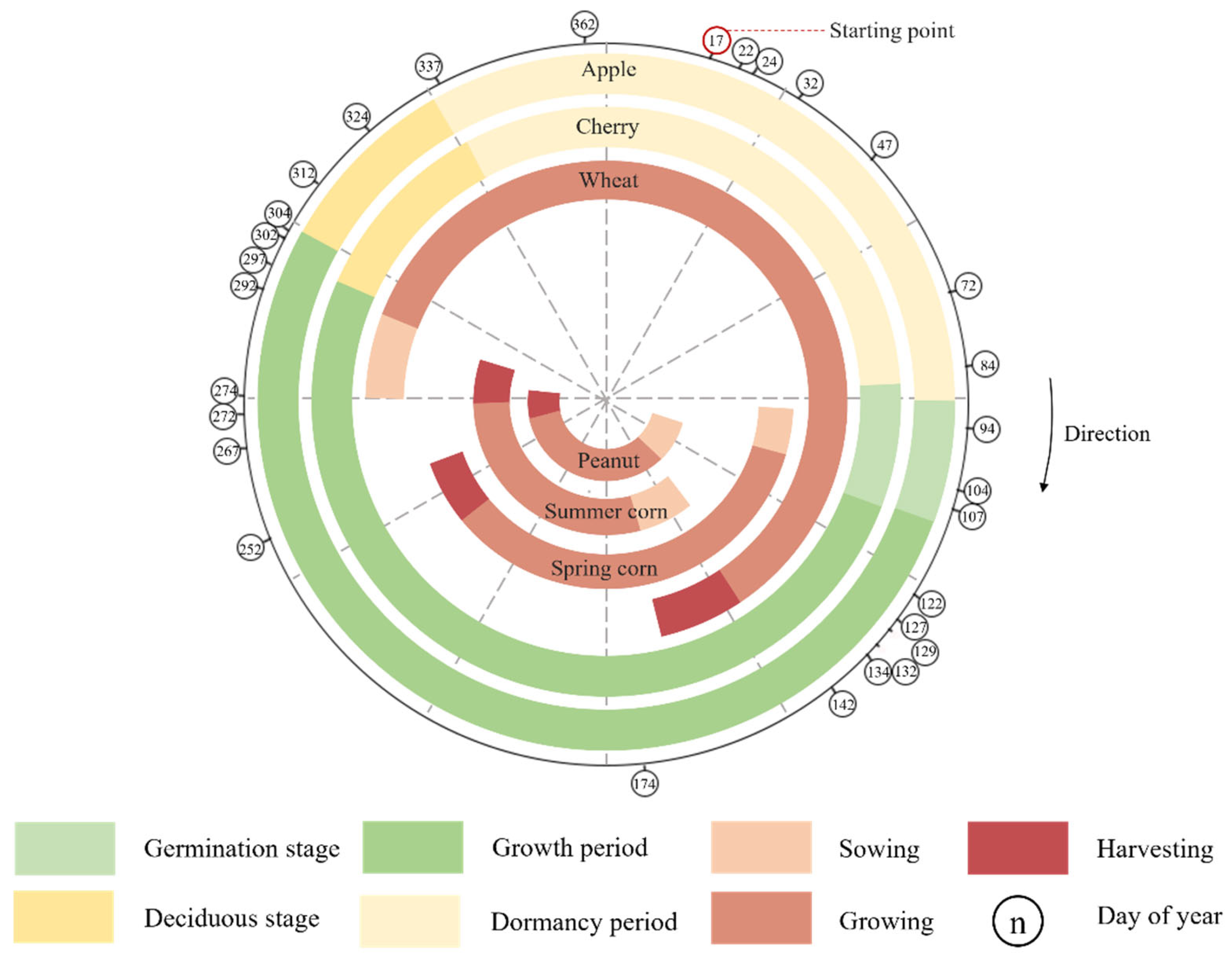
The local land cover is mainly farmland, forest land, grassland, buildings, and water. Affected by the terrain, crops are mainly planted on terraces, hills, mountains, and plains, forming a complex and diverse agricultural landscape. The agricultural economy mainly comes from horticultural crops, mainly rich in apples and cherries. It is also the seedling base of these two fruit trees. These two horticultural crops are both Rosaceae plants and deciduous trees. Therefore, the phenological similarity between the two crops is very high. In addition, there are a small number of wheat, corn, peanuts, and other crops. According to the field investigation, the crops were divided into apple orchards, cherry orchards, seedlings, and greenhouses. Phenological information for different crops is presented in Figure 2. The figure also shows the acquisition time of the regular time series images.
The best time to identify apple and cherry orchards is in late autumn. During this period, the distribution of fruit trees can be clearly seen in the VHR images (Figure 1). The ground background of the fruit trees becomes soil, and the boundaries of parcels can be clearly identified without being affected by the crowns of the fruit trees.

2.2. Remote Sensing Data

Google satellite images (VHR images) are selected to extract farmland parcels. The spatial resolution is 0.55 m, which provides three bands of red, green, and blue, including rich texture features. In terms of visual effects, we can clearly see the spatial distribution of the agricultural parcels.
Sentinel-2 optical images are used to construct time-series features for classification. The Sentinel-2 satellite consists of a multispectral imager that includes the Sentinel-2a and Sentinel-2b satellites. The revisit period was less than 5 days. From the visible band to the short-wave infrared band, the following spatial resolutions can be observed: 10 m, 20 m and 60 m. In this study, visible and near-infrared bands with a spatial resolution of 10 m are used, as shown in Table 1. Sentinel-2 satellites have the advantages of a high spatial-temporal resolution, rich spectral information, and low acquisition cost, which can provide long-term observation data for crop classification. Considering that the orchard crops are perennial plants and their phenological characteristics have been reflected throughout the year, the date range of our image selection is the whole year of 2019.
Considering that a large amount of data processing, management, and analysis work is required in the study, remote sensing data of Sentinel-2 were obtained using the Google Earth Engine (GEE) platform. GEE is a cloud computing platform that specifically processes satellite images and other earth observation data [34]. Level-2A images with radiometric calibration and atmospheric correction can be directly obtained from GEE. For downloaded data, UTM projection is used for re-projection.

2.2.1. Regular Time Series Image

Regular time series require the time series to be of the same length at different spatial locations in the study area. Therefore, when the regular time series were built, the whole study area was taken as the screening range, and the images with less than 20% cloud cover were selected. A total of 29 high-quality Sentinel-2 images covering the study area were obtained. The date distribution of these images is marked in Figure 2.
In general, 29 images should be enough to provide data support for crop classification. However, this conclusion is not applicable in our study area. The main reason is that the distribution date of these images is irregular. In most months, there are two or three images. In October, there are five images. In May, the number of images reached six. In these months, images are sufficient to describe the characteristics of crop growth. However, there is only one in June, and no image is available between July and August. In fact, this period is the key growth period for fruit trees. During this period, the lack of images will lead to a decline in the classification accuracy of orchards [21].

2.2.2. Irregular Time Series Image

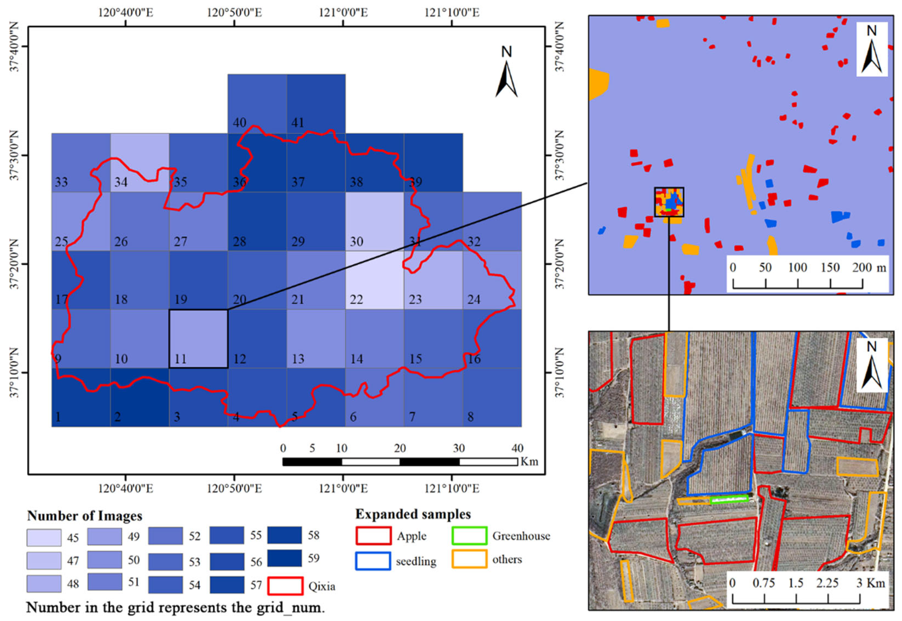
When acquiring images of irregular time series, the study area is divided into several regular grids, and each grid cell will be used as the basic unit for the subsequent acquisition of irregular time series images. The smaller the grid area, the higher the utilization rate of fragmented optical data. However, with the refinement of the grid area, this will bring higher computational pressure and resource consumption. Considering the area of the study region and the data quality factors, Qixia City is divided into 41 grids with a size of 9 km × 9 km. The grid division result is shown in Figure 3.
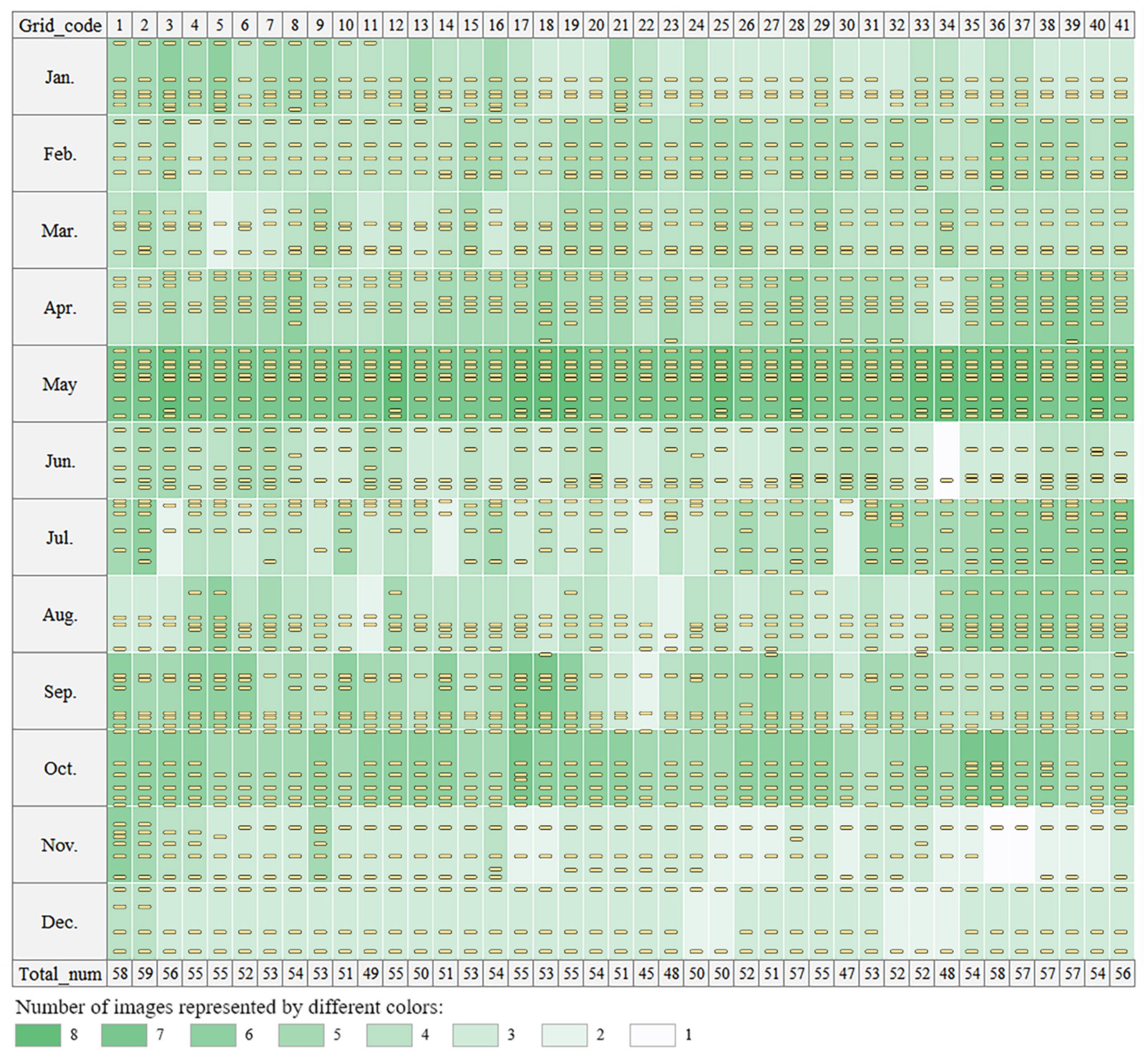
GEE supports free Sentinel-2 images. When selecting data, each grid is used as a cell for data filtering. First, all Sentinel-2 images in the grid for 2019 are acquired, and then cloud amount statistics are carried out on these images with the quality control band (QA) [35]. Cloud amount screening is carried out with 10% as the threshold value. Images less than this threshold value will be used as the data source for the subsequent construction of the crop growth curve, and images greater than this threshold value will be discarded. In the process of image selection, the number and acquisition date of images in different grids will be different, which results in an irregular time series for the whole study area (Figure 4).
As can be seen from Figure 4, the number of images in the irregular time series is greater than that in the regular time series. Among the 41 grids, the number of available images in the 22nd grid is the lowest, with only 45 images. Grid 2 has the largest number of available images, with 59. The irregularity of images between different grids is not only reflected in the number but also in the acquisition date of available images, especially in June, July, and August. Compared with the regular series, the irregular time series has more available data between these three months (the key growth period of fruit trees), which can provide more abundant characteristics for the crop growth curve.

2.3. Field Survey Data

To obtain the training and validation samples of crop classification in the study area, a field survey was conducted in the middle of May 2021. GPS-enabled devices were used to collect the geographical coordinates of samples and the corresponding crop categories. In the study area, a total of 1568 samples were collected, including 1260 apple orchard samples, 109 cherry orchard samples, 131 seedling samples, and 68 greenhouse samples. The spatial distribution of samples is shown in Figure 1. Outdoors, the positioning error of the device was less than 1 m. During sampling, large parcels were mainly selected, and sample points were collected in the centers of the parcels to ensure that the distribution of samples was not affected by positioning errors.
The samples obtained from the field survey are shown in points. In order to obtain more data for model training, the point samples were expanded. On the VHR images, the point feature is expanded into the polygon feature according to the parcel range, as shown in Figure 3. Then, the pixels in the polygon are randomly selected as sample data. A total of 54,815 samples were obtained. A total of 80% (43,852) of them were used for model training, and 20% (10,963) were used for accuracy evaluation. In addition to the four types of crops, the “other” label was set during model training to deal with other surface covers (buildings, water, staple crops, bare soil, etc.). Because these land use types have strong texture features in high-resolution images, the samples labeled “other” were selected through visual interpretation. A total of 54,765 samples labeled “other” were randomly selected from polygons. The number of training data and validation data of different categories is shown in the Table 2.

3. Method

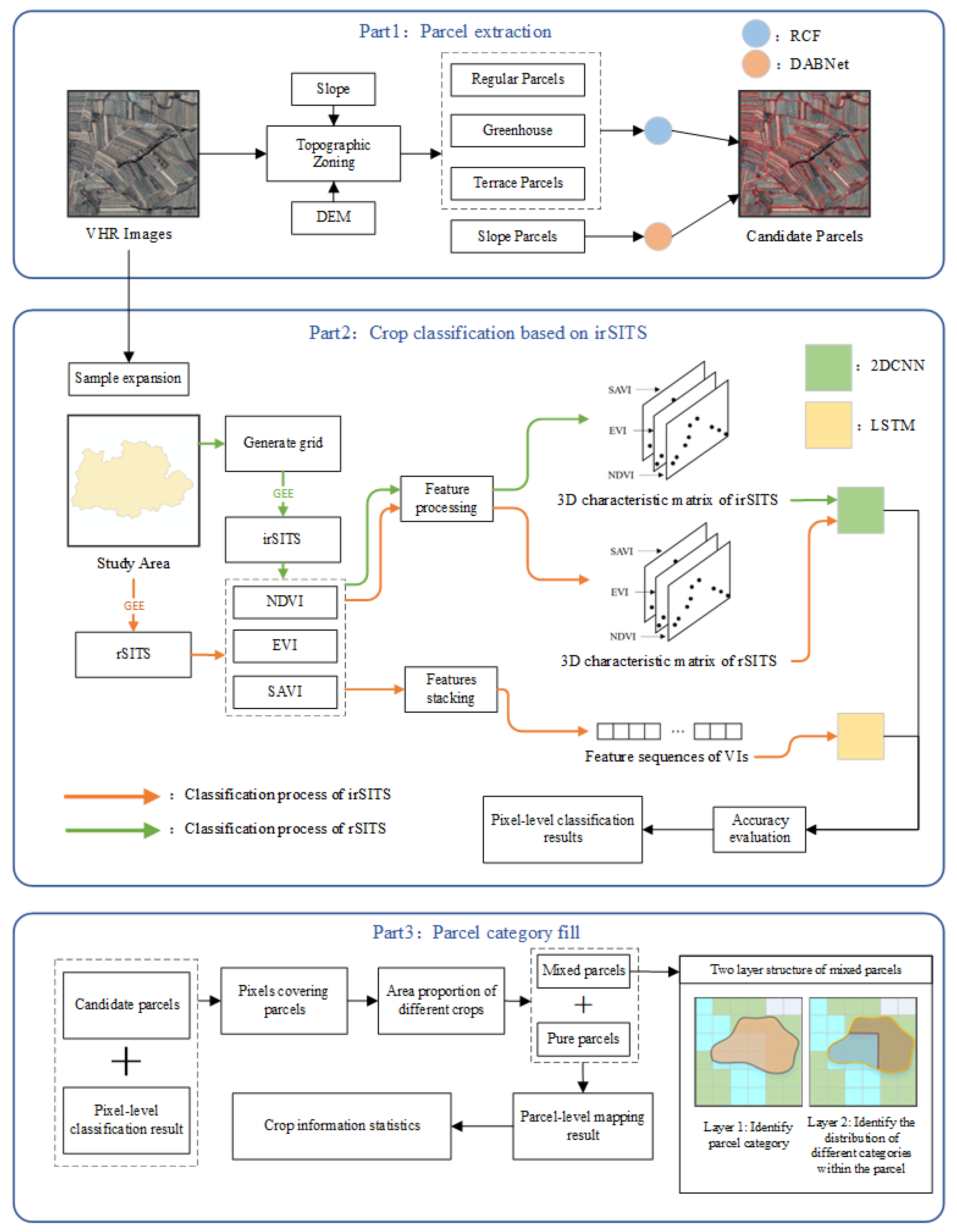
In this study, a parcel-level mapping method of a horticultural crop planting structure is proposed based on irregular time series features in complex mountainous areas covered by clouds. This section will describe the architecture of the method used in detail. Figure 5 illustrates the specific flow chart of this method, which mainly includes three parts.
  • Parcel extraction framework based on VHR images. Taking Google Earth images as the data source, the candidate parcels in the study area are extracted using the geographical idea of zoning and hierarchical strategies and the deep learning algorithms.
  • Crop classification based on irregular time series. Based on the Sentinel-2 images, the irregular time series growth characteristics of crops are constructed, and the 2DCNN algorithm is used to classify the horticultural crops;
  • Parcel-type filling. In view of the complex agricultural planting situation in the study area, a parcel-type filling strategy is designed. According to the filling strategy, the optimal classification result obtained in the second part is used to obtain the parcel category, and finally the parcel-level orchard crop planting structure mapping is realized.

3.1. Parcel Extraction Based on Hierarchical Extraction Scheme

Accurate extraction of farmland parcels is the first step toward realizing parcel-level crop planting structure mapping. In the method presented in this paper, the scheme of zoning and stratification and deep learning algorithms were used to extract farmland parcels in the study area.
Due to the influence of topographic factors, the characteristics of the spatial structure of cultivated land objects in mountainous areas show great differences [21]. This complexity will reduce the extraction accuracy of the algorithm. It is unreasonable to use only one classification algorithm (either an edge-based model or a texture-based model) to extract the parcels in the whole complex area. The zoning and hierarchical extraction scheme can solve this problem well. The concepts of zoning and hierarchical extraction simulate the image cognitive process of human vision and consider the additional spatial information suitable for large-scale geographical entity perception, which makes the land cover classification process hierarchical. The application ideas of zoning and stratification have shown good results in many previous studies [36,37,38,39].
When the extraction method is applied, different strategies should be designed for specific geographical environments. As shown in the Table 3 according to the topographic conditions of Qixia City, firstly, the study area is divided into a mountainous area and a plain area by using elevation and slope data. The plain area includes regular parcels and greenhouses, and the mountainous area includes slope parcels and terrace parcels. The main difference between these two parcels is whether the terrain has been artificially modified. The extraction model can be constrained to a stable and unified region for feature learning and reduce the probability of false detection.
Two deep learning algorithms are used to extract parcels, namely the RCF model and the DABNet model. The RCF network is a type of deep learning network based on edge features [40]. In essence, it is a convolutional neural network. It can learn rich edge information from images and is used to extract regular parcels, greenhouses in plain areas, and terraced parcels in mountain areas.
The predicted output of RCF is the probability that the pixel is the edge of the parcel, with a range of 0–1. The larger the value, the higher the probability that the pixel is the edge of the parcel. The parcel edge can be extracted by setting a reasonable threshold value for the raster transformation vector.
DABNet is a lightweight semantic segmentation model, which can ensure the extraction effect and the training speed [41]. It can learn the texture information of the image and distinguish the hillside parcels and forest areas without clear edge boundaries. The main research object of this paper (apple and cherry orchards) has similar phenological characteristics to natural forests [21]. Therefore, forests will interfere with the accuracy of the classification results based on the time series classification models. However, there is a large gap in texture between horticultural crops and natural forests. When using DABNet to extract hillside parcels, forest land can be extracted using texture information for masking; this can avoid the interference of natural forests in orchard classification.
In the process of model training, it is necessary to conduct model training and parcel extraction for different zones. The prediction results of these two models are raster data, which need to be converted into vector elements to obtain the parcel polygon. The parcels obtained at this time are not all farmland parcels, so we call them candidate parcels. It is also necessary to filter candidate parcels according to the crop classification results to obtain farmland parcels.

3.2. Classification Method Based on Irregular Time Series

3.2.1. Classification Feature Selection

In this paper, the time series vegetation indexes for crops are used to characterize crop growth patterns. The characteristics of vegetation indexes are calculated for the regular and irregular time series. Due to the algebraic operation between different bands, vegetation indexes can be generated to better reflect vegetation growth and soil conditions. According to the vegetation status of the study area, three vegetation indexes were selected: the normalized differential vegetation index (NDVI) [42], the enhanced vegetation index (EVI) [43], and the soil regulation vegetation index (SAVI) [44].
NDVI and EVI are more sensitive to the difference when the vegetation biomass is low or high [25]. SAVI is more able to reflect the soil background of orchard crops and is suitable for describing the difference in soil background during the growth of horticultural crops [44]. A previous study has demonstrated their usefulness in the classification of garden crops [21].
The formulas for these vegetation indexes are as follows:
N D V I = N I R R N I R + R
E V I = 2.5 × N I R R N I R + 6 R 7.5 B + 1
S A V I = 1 + L N I R R N I R + R + L
NIR is the near infrared band, R is the red band, B is the blue band, and L is the soil regulation coefficient, which is taken as 0.5 in this paper.

3.2.2. Irregular Time Series

The irregular time series in this study is defined as satellite image time series with an inconsistent composition of effective observation time series in the study area. Irregular time series can make full use of fragmented high-quality remote sensing images, avoid the unavailability of images for the whole period caused by cluster clouds, and are more conducive to the construction of the time series growth characteristics of crops.
Figure 6 shows the concept of irregular time series. The matrix represents the time series with the effective observation of pixels in the study area during the study period. For one pixel, “1” means that there is an available image at time t . “0” means that no image is available at time t . The black boundary around each image represents the boundary of this image. The blank area in the image represents that the image in this area is missing at this time due to cloud cover. The main reasons for the existence of irregular time series are as follows:
  • Overlapping area between different strips. The observation range of remote sensing satellites generally overlaps between different strips. The number of images in the overlapping area is higher than that in the non-overlapping area;
  • Cloud cover. Clouds on optical images will seriously affect the image quality, and the number of effective observations will be different in areas covered by cloud and those without cloud;
  • Scale of the study area. For study areas with different scales, the number of images that need to be covered is different. If these images are in different bands, image acquisition dates will vary.
In this study, there are three situations for the existence of irregular time series:
  • The number of time series images in different grids is the same, but the image acquisition date is different, such as A and B in Figure 6;
  • The image acquisition date is the same, but the total number is different, such as A and E in Figure 6;
  • The number of time series images is different, and the image acquisition date is also different, such as A and C, D and F.

3.2.3. 2DCNN for Irregular Time Series

François Petitjean [30] once divided the classification work based on time series into three levels according to the degree of mining time series information by the model in the supervised classification process. In the first level, time is only used as an image identifier, and satellite images have no constraint relationship with each other. The change in image order will not affect the classification result. In the second level, considering the constraint between two times, time exists in pairs. In the third level, the images are arranged in time series. In the third level, the images should be organized strictly by time, with no confusion allowed. Obviously, with the improvement in the level, the model gradually deepened the mining of time series information. However, few algorithms in existing crop classification research can reach the third level of time series data mining. At present, machine learning and recurrent neural networks are the main classifiers used in classification research, such as RF, SVM, and LSTM. These classifiers require consistent feature lengths of input samples—that is, they can only handle the case of regular time series. Moreover, their mining of time series information is only at the first level, and they cannot extract the pattern feature information of time series data in the temporal dimension.
To solve these problems, a two-dimensional convolutional neural network is used as a classifier in this work. In particular, 2DCNN is widely used in computer vision and image recognition. In the field of agricultural remote sensing, some scholars also use 2DCNN to carry out related research [45,46]. Mahesh Pal et al. [47] compared the classification performances of SVM, NN, and 2DCNN, and the results showed that the classification effect based on 2DCNN was better than it was for the other two, which indicated the superiority of 2DCNN. The inputs of 2DCNN are images, while the basic unit in the process of crop classification is a pixel, which is a one-dimensional feature. Therefore, the primary task of crop classification using 2DCNN is the format conversion of pixel-level feature sequences into a feature matrix.
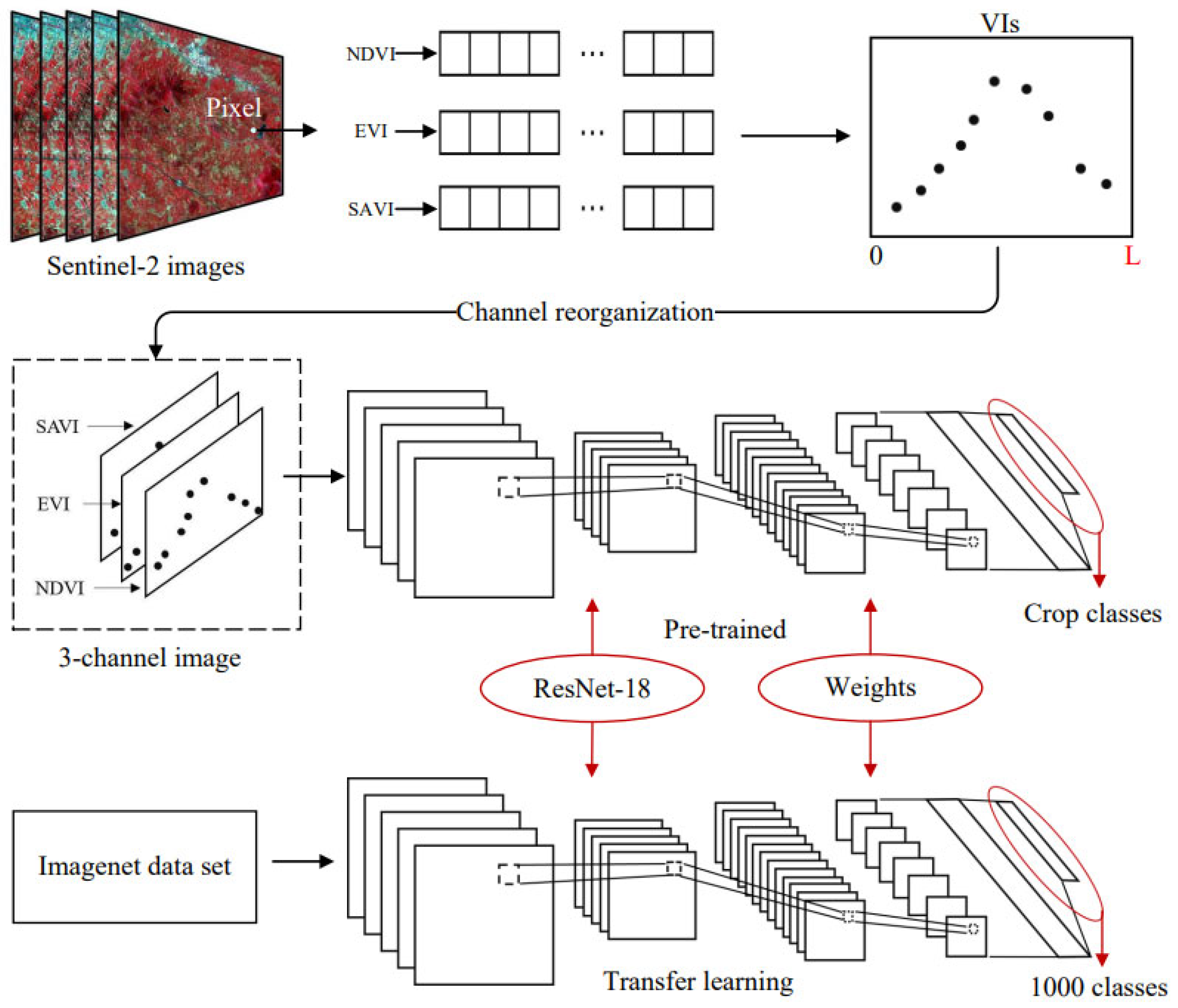
Diyou Liu [48] proposed a format conversion method for a one-dimensional irregular time series. In this study, a two-dimensional matrix for time is constructed for each pixel, and then the input structure (three-dimensional matrix) of 2DCNN is obtained by channel reconstruction. The flow chart is shown in Figure 7. This process mainly includes two steps:
(1) For each pixel, the irregular time series features are extracted from the original optical image and transformed into a two-dimensional matrix representing the phenological characteristics of crop growth. For each pixel, the values of NDVI, EVI, and SAVI are calculated. By stretching the one-dimensional time series and taking the study period as the length of the matrix, the two-dimensional characteristic matrix is obtained. This process is mainly used to adapt to irregular time series. The formula for mapping one-dimensional features to two-dimensional features is as follows:
V I r = l × V I o r i m i n V I m a x V I m i n
Here, V I r represents the value after stretching, and l is the length of the two-dimensional matrix—that is, the time length of all available images. In this study, the time range of images used is from 2 January to 28 December 2019, so l is equal to 360. In the two-dimensional eigenmatrix, the horizontal axis represents time, and the vertical axis represents the index value. Irregular time series are regularized by mapping features from one dimension to two dimensions.
(2) The feature matrix obtained in the first step is reconstituted as the model input of 2DCNN in this step. The matrix obtained based on the three indexes is used as the RGB band of the true color image to obtain the 3D matrix suitable for 2DCNN. The neural network can extract the temporal pattern change. The 2DCNN used in this study is a lightweight and efficient Resnet-18 model of classical residual network series, and the model pre-trained on the ImageNet dataset is used for transfer learning training.

3.2.4. Contrast Experiment

To verify the effectiveness of the classification method based on irregular time series, two groups of comparative experiments are set up in this work. The 2DCNN and LSTM algorithms are used to classify regular time series.
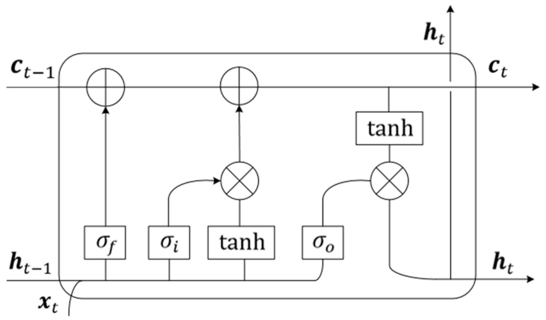
LSTM is proposed based on the Recurrent Neural Network (RNN) [49]. A unique structure is designed in the LSTM network (Figure 8) that can solve the problem of gradient disappearance or explosion in the training process by controlling the state of error flowing through the structure. It is a neural network model that can be used to process and predict time series. LSTM works well over a broad range of parameters, such as the learning rate, input gate bias, and output gate bias. The number of hidden layers and the number of neurons are important parameters in LSTM and have a great impact on the classification performance. In this study, 2 network layers and 32 neurons are set as the optimal network parameter configuration [21].

3.3. Classification Result Filling Strategy

At present, the commonly used method to determine the farm parcel category is mainly to take the parcel as the unit of classification, take the average value of the pixel features within the parcel as the characteristics of the parcel, and then use the supervised classifiers to classify the parcel category [37,50,51,52,53,54]. This method assumes that there is only one crop in the parcels. In fact, in actual agricultural work, there are complex planting situations, and it cannot be guaranteed that there is only one type of crop in one parcel—that is, the parcel is a mixed parcel [55,56]. The main reasons for the existence of mixed parcels in the study area are as follows:
  • Typical mixing in the study area. The study area is a typical small farm planting area, and the orchard does not have the capacity for scientific planting planning. The market value of cherries is higher than that of apples. Farmers take economic benefits as the leading factor in the adjustment of the planting structure, and they gradually plant many cherry trees in apple orchards. However, there is no obvious regular boundary between cherry trees and apple trees, which leads to the phenomenon of mixed parcels.
  • In VHR images, the texture of apple orchards and cherry orchards is very similar. When extracting parcels from slope areas to ensure the correctness of parcel attributes, and taking these two orchards as one type, the parcel extraction experiment based on texture structure was carried out. DABNet can only obtain orchard parcels from VHR images; it cannot obtain detailed apple orchards or cherry orchards. If the model is trained with apple and cherry orchards as sample categories, the effect of parcel extraction will be greatly compromised, and many slope parcels will be over-zoned, making them very different from the actual parcels, and they will lose semantic information.
The filling strategy adopted in this study mainly takes the boundary information of candidate parcels as the spatial constraint of the pixel-level classification results, and the classification of parcels is mainly determined by the pixel-level classification results. The implementation steps are illustrated in Figure 5.
Firstly, the pixels that covered candidate parcels were obtained through the spatial overlay relationship between the parcels and the pixel-level classification results. If these pixels are all in one category, the parcel is pure, and the category is the parcel category. If they are of different categories, the parcels are judged as mixed parcels. For mixed parcels, the double-layer storage structure is used to characterize the spatial distribution of crops, as shown in Figure 5. On the first level, parcels are marked as mixed parcels. The role of the second layer is to display the crop categories and spatial distribution within the mixed parcels. With pixels as the boundary, we aim to outline the distribution positions of different crops. In the statistics of the crop planting area, the area of pure parcels is directly counted. In the mixed parcels, the area of different crops is counted separately. In this process, the error transmission of parcel extraction errors in parcel-level mapping is avoided, and some errors in the pixel-level classification results can be reduced to improve the mapping accuracy.

3.4. Accuracy Evaluation

3.4.1. Precision Evaluation of Parcel Extraction Results

For the result of parcel extraction, a precision evaluation needs to be carried out in consideration of two aspects: the boundary precision and the geometric precision of parcels. In the task of parcel extraction, it is not required that the extraction result be completely consistent with the true value of manual annotation. Although the boundary of some parcels is slightly offset from the true value, it is still consistent with the actual parcels and cannot be judged as an extraction error. Therefore, buffers of 1 m width (2 pixels) and 2 m width (4 pixels) are built around the real parcel boundary. The overlapped region of the extracted boundary and the buffers is taken as part of accurate identification. The confusion matrix of the boundary extraction results is constructed, and the F1 score is calculated based on the confusion matrix. The F1 score is the harmonic average of precision and recall. The precision is used to calculate the proportion of correct recognition in the detection results. The recall rate represents the proportion of correctly predicted boundaries to all truth boundaries. As the comprehensive value of the two, the F1 score comprehensively measures the two indicators. The higher the score, the closer it is to the optimal extraction. The relevant formulas are as follows:
recall = TP TP + FN
precision = TP TP + FP
F 1 = 2 × recall × precision recall + precision
TP represents the correctly identified boundary. FP represents the error part of the extraction result. FN represents the recognized part of the real boundary. F1 is used as the global boundary precision indicator.
To consider the geometric accuracy of the extracted parcel, the area-based intersection union ratio (IoU) index is used to measure the fit level between the extracted parcels and the actual parcels.
IoU = A B A B
A is the area of the extracted parcels, and B is the area of real parcels.

3.4.2. Precision Evaluation of Classification Results

Based on the sample data, the confusion matrix was constructed for different classification results, and the overall accuracy and K a p p a coefficient were calculated to evaluate the classification accuracy [14].

4. Result

4.1. Candidate Parcel Extraction Results

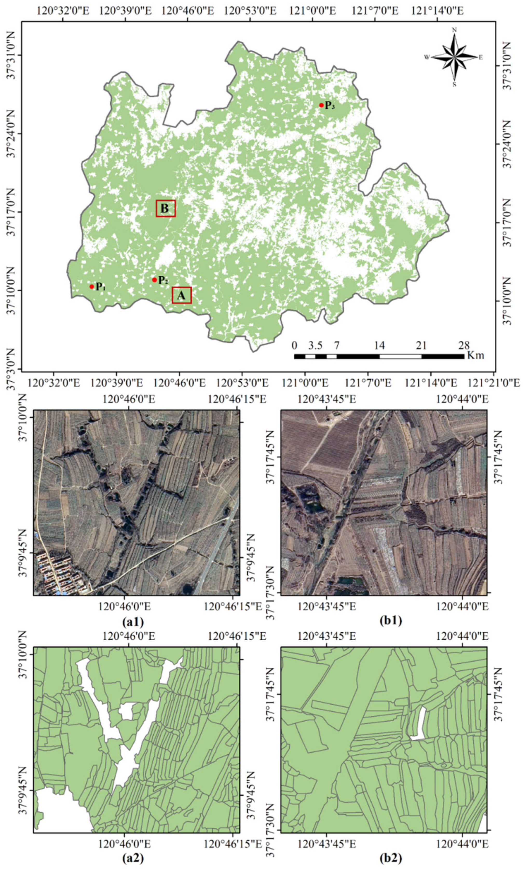
The candidate parcels in the study area are obtained based on the parcel extraction framework of zoning and hierarchical extraction. The distribution of parcels is shown in Figure 9. The parcels here are obtained by the vector line to polygon elements. In this process, the parcels obtained include not only farmland parcels but also non-farmland parcels. As shown in areas (a) and (b) in Figure 9, they are called candidate parcels. Candidate parcels need to be filled by crop categories to obtain the final parcel-level crop distribution map. Overall, 69,8899 candidate parcels with a total area of 129,323.7 ha were extracted.
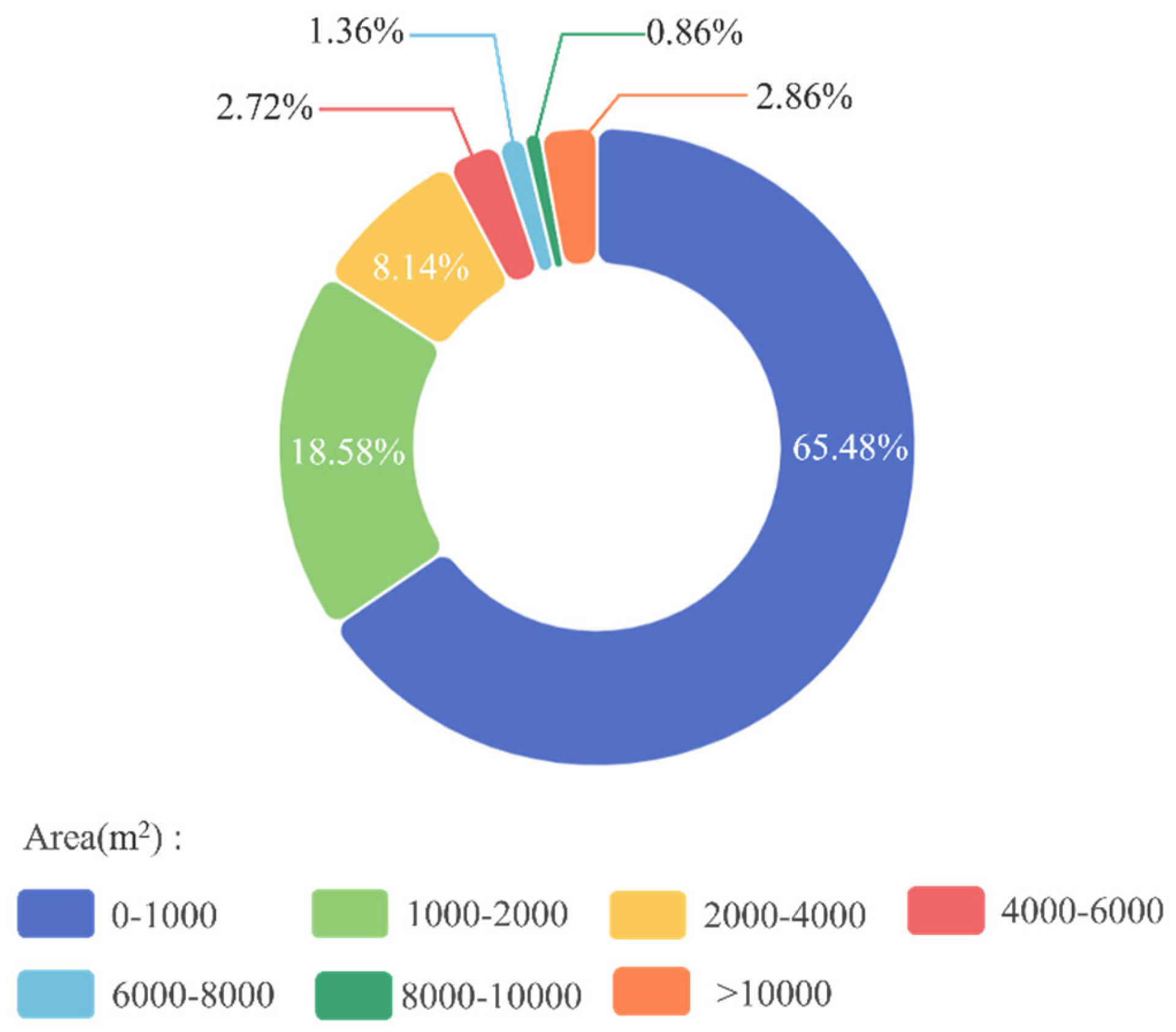
The area information of candidate parcels was statistically analyzed, as shown in the pie chart in Figure 10. It was found that 65.84% of the parcels were smaller than 1000 m2, mainly terraced parcels and some small regular parcels in the plain. Moreover, 94.92% of the parcels were smaller than 6000 m2, reflecting the characteristics of smallholder planting and parcel fragmentation in the study area. Parcels with large areas were few and were mostly distributed on the hillside. The lack of scientific management of slope parcels has led to crop mixing, especially in areas where both apples and cherries are grown [21].
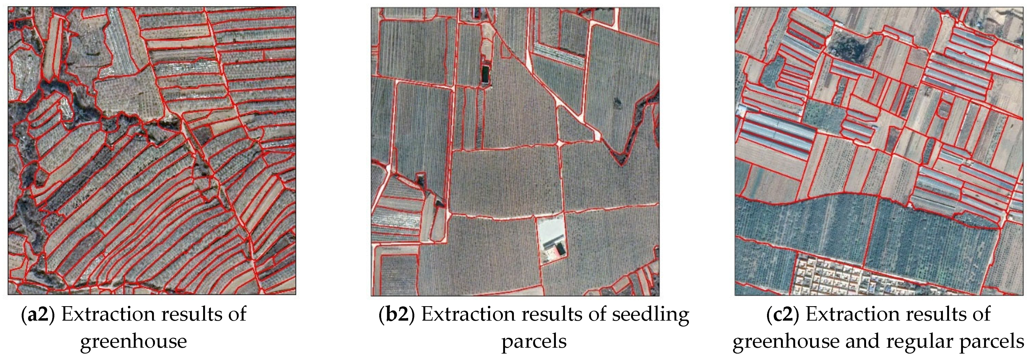
The detailed parcel extraction effect is shown in Figure 11. Compared with many traditional algorithms, it has a better extraction effect. The use of deep learning algorithm extraction can fully extract the edge information of terraced parcels. At the same time, it can be seen from (b) that this method can even avoid the interference caused by the texture, such as the edge information inside the seedling parcels, and will not cause over-extraction phenomena on this type of parcel and can identify the edge information of the greenhouse very well. Therefore, it is considered that seedling parcels and greenhouses are pure, and there is no mixed planting with the two orchards (apple and cherry). Based on this, it is believed that the mixed parcels in the study area are mainly composed of two horticultural crops: apple orchards and cherry orchards. In fact, in the field, the local planting situation is indeed the same, with mainly mixed planting among fruit trees.
In order to verify the effect of parcel extraction, the buffer zones were calculated with radius measurements of 1 m and 2 m for the boundaries. The F1 score and IOU were then calculated. The results are shown in Table 4. Evaluation of parcel extraction effect. IoU is 0.872. When the radius of the buffer zone is 1 m, the F1 score is 0.93. When the radius is 2 m, the F1 score is 0.96. The precision evaluation results show that the parcel extraction effect is sufficient to support the research on parcel-level crop mapping.

4.2. Analysis of Classification Experiment Results

Based on the experimental details elaborated in Section 3.2, three groups of classification experiments were carried out. The confusion matrix was calculated to evaluate the accuracy of different classification results. A total of 10,963 real values were used to construct the confusion matrix, including 6682 apples, 2862 seedlings, 658 cherry orchards, and 761 greenhouses. The confusion matrices are shown in Figure 12a–c.
The results show that the classification method based on irregular time series and the 2DCNN model is the best, with an overall accuracy of 97.76% and a kappa coefficient of 0.9594, which is higher than that of the other two groups of comparative experiments, indicating the effectiveness of this pixel-level crop classification method. The classification result’s precision based on regular time series and the 2DCNN model is 95.93%, and the kappa coefficient is 0.9267. The overall accuracy based on regular time series and LSTM is 94.01%, and the kappa coefficient is 0.8925. It is believed that the overall accuracy of the first two is higher than that of the LSTM classifier because, in the experiment with 2DCNN as the supervised classifier, the time series feature data of each pixel has been mapped from one dimension to two dimensions. By classifying the recognized method of each pixel, more dependencies between time series images can be learned.
According to the time series classification hierarchy proposed by François Petitjean [30], the classification method based on LSTM belongs to the first level. In the process of supervised classification feature learning, the model will not learn time information but will only stack images, and the mining of time series information occurs at a shallow level. The classification method selected in this work is based on irregular time series and 2DCNN, which maps the time series features into a two-dimensional feature matrix. In the classification process, not only can the feature information of each node be learned, but the trend information in the time series data can also be mined at a deeper level. Therefore, the accuracy of both “irregular time series +2DCNN” and “regular time series +2DCNN” is better than that of LSTM.
The overall accuracy of different grids is also calculated. Since grids 8, 35, 32, and 41 cover a small portion of the study area, the amount of verification data available from them is small and not typical. Therefore, we did not evaluate the accuracy of these four grids. We mainly evaluated the accuracy of grids with a large coverage area. The overall accuracy of different grids is shown in (d) in Figure 12. The classification accuracy of the 28th grid is the highest, at 98.7%, and that of the 22nd grid is the lowest, at 94.1%. With the increase in the number of images, the overall accuracy of the grid is gradually increased. This shows that the increase in optical images can more accurately describe the changes in biomass during the growth of the orchard, and the application of irregular time series can make full use of fragmented optical data.
The irregular time series is proposed to solve the problem of poor climate conditions, or the problems experienced in a large-scale study area, which makes it difficult to keep the length and date distribution of the regular time series of the pixels in different positions in the study area consistent. In this case, regular time series data describing surface information are obtained by filtering and pre-processing the original data from many studies. This leads to the abandonment of a lot of available optical information, which leads to the underutilization of the optical information used to describe crop growth. This leads to low classification accuracy. Classification based on irregular time series results in the extraction of the time series of different pixels separately, so optical sequences can be used as much as possible to improve the accuracy of classification results. In the research, 2DCNN is used as the classifier. This model can transform the classification task into the classification of each pixel’s three-dimensional feature map. The experimental results show that, compared with LSTM, the 2DCNN model can better extract the growth pattern of crops over the whole growth period and then achieve better classification results.

4.3. Parcel Filling Result

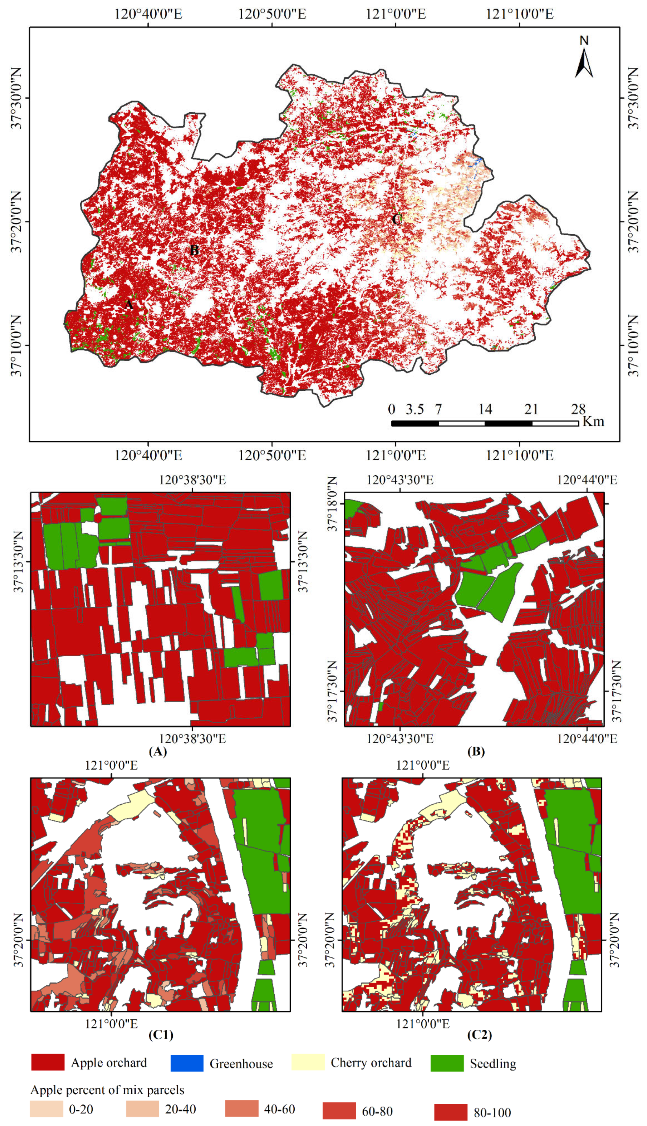
Based on the candidate parcels and pixel-level classification result of the study area, the parcel categories of the study area are filled according to the parcel filling strategy described in Section 3.3. The parcel-level mapping results for horticultural crops are shown in Figure 13. Apple and cherry orchard parcels, seedlings, greenhouses, and mixed parcels (apple and cherry mixed planting) are shown in Figure 13.
As can be seen from Figure 13, apple orchards are distributed throughout the study area, but are mainly distributed in the hilly areas in the southwest and west of the study area and the central plain area. Seedling parcels are mainly distributed in the west, southwest, and north of the relatively flat terrain. Greenhouses are mainly distributed in the north and east of the study area. Cherry orchards are mainly found in the eastern and northeastern mountains, and many of them exist as mixed parcels. According to the statistical yearbook data of Qixia City in 2019 [57], cherry orchards are mainly distributed in Shewopo Town, Tangjiapo Town, Taocun Town, and Miaohou Town (east and northeast of the study area) in Qixia City, which is consistent with the classification results of this study. This further demonstrates the effectiveness of the proposed method.
Total area of apple orchard:
A a = A a 1 + A a 2
Total area of cherry orchard:
A c = A c 1 + A c 2
For mixed parcels, different colors are chosen to represent them according to the proportion of apples in parcels. The darker the color, the higher the proportion of apple trees. A sub-region of mixed parcels is selected to realize the two-layer structure of mixed parcels. According to the result, we applied statistics to the planting information in the study area, and the results are shown in Table 5. A total of 470,539 farm parcels were obtained, with a total area of 93,180 hectares. There are 415,233 apple orchard parcels, 19,455 cherry orchard parcels, 1096 greenhouses with an area of 82.2 ha and an average area of 750.3 m2, 4031 seedling parcels with an area of 3121.3ha and an average area of 7743.1 m2, and 30,724 mixed parcels. After calculation, it is found that 84,212.4 ha of apple orchards and 5764.3 ha of cherry orchards are planted in the study area.

5. Discussion

In this study, a parcel-level mapping method for perennial orchard crops was proposed. Experiments show that this method has good classification accuracy in complex planting scenes and can significantly solve the problem of insufficient images. Several contributions can be drawn from our study.
  • Based on the method proposed in this study, parcel-level orchard mapping experiments were successfully carried out in smallholder agricultural areas, and it was demonstrated that parcel-level mapping results can provide more abundant crop planting information than pixel-level classification results.
  • Irregular time series are used to construct crop growth characteristics. The classification results show that this method can make full use of optical image information and can solve the problem of missing data in key growth periods in regular time series. The feature mining of time series data is promoted from the first layer to the third layer, and the dependence between time series can be deeply mined.
  • The extraction result of the parcels is only used as the spatial constraint of the pixel-level result, to avoid the impact of the error of parcel extraction on the final mapping result. Considering the possible mixed planting situation in parcels, the obtained statistical information has higher accuracy.
Taking Qixia City, Shandong Province, China, as the research area, relevant experiments were carried out. The results show that the parcel-level mapping method based on irregular time series and VHR images proposed in this paper shows good performance in horticultural crop mapping in complex mountain areas. However, after discussion and analysis, it was found that this method still has some problems, which can be addressed in future work.
  • The requirements for sample distribution are higher. Irregular time series are built independently in each grid. Within the grid, the time series characteristics (length, date distribution) are consistent. This requires that when preparing sample data, there should be a distribution of the sample data in each grid. Therefore, the question of how to enhance the model to learn more detailed and profound features between the different grid time series is the focus of future research.
  • The 2DCNN model is used in the classification. In order to obtain the input format supported by the model, the time series data are stretched into a three-dimensional image. During this process, the sparse matrix is obtained. Although the classification effect has been optimized, there is still room for improvement. It is believed that if the feature matrix can be supplemented with information by fusing SAR data and other multi-source data, better classification results will be achieved.

6. Conclusions

In the process of parcel-level orchard crop mapping in mountainous areas, it is difficult to obtain sufficient optical images to describe the growth characteristics of crops in the key growth period (June to August) due to clouds and rain. In view of this problem, this paper proposes a method to realize the construction of time series characteristics and the complete parcel-level mapping of orchards. The core idea of this method includes three parts: parcel extraction based on a hierarchical extraction scheme, crop classification based on irregular time series and the 2DCNN model, and parcel category filling.
Based on VHR images and time series Sentinel-2 data, parcel-level mapping experiments on horticultural crops were carried out in Qixia City, Shandong Province, China. The method showed good extraction performance. According to visual inspection, the parcel extraction strategy based on the hierarchical extraction scheme can achieve a good extraction effect. In the research area, three groups of classification experiments were carried out, namely “irregular time series + 2DCNN,” “regular time series + 2DCNN,” and “regular time series + LSTM”. Among the three groups of experimental results, the classification of irregular time series based on 2DCNN had the highest accuracy. The overall accuracy was 97.76%, and the kappa coefficient was 0.9594. This showed the effectiveness of the classification method adopted in this study. This method can improve the efficiency of the use of fragmented optical information and upgrade the time series classification model from the first level (where time is only used as an identifier) to the third level, which can aid in learning the deep time constraint information.
In fact, it is believed that the classification method based on irregular time series can not only be used for the classification of horticultural crops but also for the extraction of surface information in many cloudy and rainy areas.
In future work, the question of how to explore more farmland parcel extraction methods and optimize the large-scale parcel extraction effect is an important problem to be solved. In addition, the question of how to fuse multi-source optical and SAR to supplement irregular time series information to improve classification accuracy is also an important research direction to be considered in the future.

Author Contributions

S.J. proposed the methodology, prepared the data, performed, and analyzed the experiments, and wrote the manuscript. W.K. helped modify models. S.J., H.W., W.K. and Z.J. helped conduct the field investigation and experiments. Z.S. outlined the research topic, acquired the funding and revised manuscript. S.J., J.L. and Y.L. helped prepare sample data. All authors have read and agreed to the published version of the manuscript.

Funding

National Key Research and Development Program of China (2021YFC1523503), the third comprehensive scientific expedition to Xinjiang (2021xjkk1403), National Natural Science Foundation of China (41971375), and the Key Research and Development Program of Xinjiang Uygur Autonomous Region, grant number (2022B03001-3).

Data Availability Statement

Data sharing is not applicable to this article.

Conflicts of Interest

The authors declare no conflict of interest.

References

  1. Kozhoridze, G.; Orlovsky, N.; Orlovsky, L.; Blumberg, D.G.; Golan-Goldhirsh, A. Classification-based mapping of trees in commercial orchards and natural forests. Int. J. Remote Sens. 2018, 39, 8784–8797. [Google Scholar] [CrossRef]
  2. National Bureau of Statistics. Available online: http://www.stats.gov.cn/ (accessed on 1 October 2022).
  3. Zhu, Y.; Yang, G.; Yang, H.; Wu, J.; Lei, L.; Zhao, F.; Fan, L.; Zhao, C. Identification of apple orchard planting year based on spatiotemporally fused satellite images and clustering analysis of foliage phenophase. Remote Sens. 2020, 12, 1199. [Google Scholar] [CrossRef] [Green Version]
  4. Pluto-Kossakowska, J. Review on multitemporal classification methods of satellite images for crop and arable land recognition. Agriculture 2021, 11, 999. [Google Scholar] [CrossRef]
  5. Wang, Y.L.; Xu, X.G.; Huang, L.S.; Yang, G.J.; Fan, L.L.; Wei, P.F.; Chen, G. An improved casa model for estimating winter wheat yield from remote sensing images. Remote Sens. 2019, 11, 1088. [Google Scholar] [CrossRef] [Green Version]
  6. Laneve, G.; Luciani, R.; Jahjah, M. A multi-temporal phenology based classification approach for crop monitoring in Kenya. S. Afr. J. Geomat. 2019, 8, 249–264. [Google Scholar] [CrossRef]
  7. Patel, N.R.; Bhattacharjee, B.; Mohammed, A.J.; Tanupriya, B.; Saha, S.K. Remote sensing of regional yield assessment of wheat in Haryana, India. Int. J. Remote Sens. 2006, 27, 4071–4090. [Google Scholar] [CrossRef]
  8. Phiri, D.; Simwanda, M.; Salekin, S.; Nyirenda, V.R.; Murayama, Y.; Ranagalage, M. Sentinel-2 data for land cover/use mapping: A review. Remote Sens. 2020, 12, 2291. [Google Scholar] [CrossRef]
  9. Ji, S.P.; Zhang, C.; Xu, A.J.; Shi, Y.; Duan, Y.L. 3D Convolutional neural networks for crop classification with multi-temporal remote sensing images. Remote Sens. 2018, 10, 75. [Google Scholar] [CrossRef] [Green Version]
  10. Koirala, A.; Walsh, K.B.; Wang, Z.L.; McCarthy, C. Deep learning–method overview and review of use for fruit detection and yield estimation. Comput. Electron. Agric. 2019, 162, 219–234. [Google Scholar] [CrossRef]
  11. Zhong, L.H.; Hu, L.N.; Zhou, H. Deep learning based multi-temporal crop classification. Remote Sens. Environ. 2019, 221, 430–443. [Google Scholar] [CrossRef]
  12. Kussul, N.; Lavreniuk, M.; Skakun, S.; Shelestov, A. Deep learning classification of land cover and crop types using remote sensing data. IEEE Geosci. Remote Sens. Lett. 2017, 14, 778–782. [Google Scholar] [CrossRef]
  13. Zhu, X.X.; Tuia, D.; Mou, L.C.; Xia, G.S.; Zhang, L.P.; Xu, F.; Fraundorfer, F. Deep learning in remote sensing. IEEE Geosci. Remote Sens. Mag. 2017, 5, 8–36. [Google Scholar] [CrossRef] [Green Version]
  14. Wei, L.; Jian, W.; Jiancheng, L.; Zhifeng, W.; Jingdong, C.; Yanan, Z.; Yingwei, S.; Zhanfeng, S.; Nan, X.; Yingpin, Y. Farmland parcel mapping in mountain areas using time-series SAR data and VHR optical images. Remote Sens. 2020, 12, 3733. [Google Scholar] [CrossRef]
  15. Duro, D.C.; Franklin, S.E.; Dube, M.G. A comparison of pixel-based and object-based image analysis with selected machine learning algorithms for the classification of agricultural landscapes using SPOT-5 HRG imagery. Remote Sens. Environ. 2012, 118, 259–272. [Google Scholar] [CrossRef]
  16. Ok, A.O.; Akar, O.; Gungor, O. Evaluation of random forest method for agricultural crop classification. Eur. J. Remote Sens. 2012, 45, 421–432. [Google Scholar] [CrossRef]
  17. Su, T.F.; Zhang, S.W. Object-based crop classification in Hetao plain using random forest. Earth Sci. Inform. 2021, 14, 119–131. [Google Scholar] [CrossRef]
  18. Pena-Barragan, J.M.; Ngugi, M.K.; Plant, R.E.; Six, J. Object-based crop identification using multiple vegetation indices, textural features and crop phenology. Remote Sens. Environ. 2011, 115, 1301–1316. [Google Scholar] [CrossRef]
  19. Haoyu, W.; Zhanfeng, S.; Zihan, Z.; Zeyu, X.; Shuo, L.; Shuhui, J.; Yating, L. improvement of region-merging image segmentation accuracy using multiple merging criteria. Remote Sens. 2021, 13, 2782. [Google Scholar] [CrossRef]
  20. Hossain, M.; Chen, D. Segmentation for object-based image analysis (obia): A review of algorithms and challenges from remote sensing perspective. J. Math. 2019, 150, 115–134. [Google Scholar] [CrossRef]
  21. Jiao, S.; Hu, D.; Shen, Z.; Wang, H.; Dong, W.; Guo, Y.; Li, S.; Lei, Y.; Kou, W.; Wang, J.; et al. Parcel-level mapping of horticultural crop orchards in complex mountain areas using VHR and time-series images. Remote Sens. 2022, 14, 2015. [Google Scholar] [CrossRef]
  22. Feng, S.W.; Zhao, J.J.; Liu, T.T.; Zhang, H.Y.; Zhang, Z.X.; Guo, X.Y. Crop type identification and mapping using machine learning algorithms and sentinel-2 time series data. IEEE J. Sel. Top. Appl. Earth Obs. Remote Sens. 2019, 12, 3295–3306. [Google Scholar] [CrossRef]
  23. Arun, P.V.; Karnieli, A. Deep learning-based phenological event modeling for classification of crops. Remote Sens. 2021, 13, 2477. [Google Scholar] [CrossRef]
  24. Sakamoto, T. Early Classification method for US corn and soybean by incorporating MODIS-estimated phenological data and historical classification maps in random-forest regression algorithm. Photogramm. Eng. Remote Sens. 2021, 87, 747–758. [Google Scholar] [CrossRef]
  25. Ren, T.; Liu, Z.; Zhang, L.; Liu, D.; Xi, X.; Kang, Y.; Zhao, Y.; Zhang, C.; Li, S.; Zhang, X. Early Identification of Seed Maize and Common Maize Production Fields Using Sentinel-2 Images. Remote Sens. 2020, 12, 2140. [Google Scholar] [CrossRef]
  26. Russwurm, M.; Korner, M. Temporal Vegetation Modelling using Long Short-Term Memory Networks for Crop Identification from Medium-Resolution Multi-Spectral Satellite Images. In Proceedings of the 30th IEEE/CVF Conference on Computer Vision and Pattern Recognition Workshops (CVPRW), Honolulu, HI, USA, 21–26 July 2017; pp. 1496–1504. [Google Scholar]
  27. Blaes, X.; Vanhalle, L.; Defourny, P. Efficiency of crop identification based on optical and SAR image time series. Remote Sens. Environ. 2005, 96, 352–365. [Google Scholar] [CrossRef]
  28. Hao, P.Y.; Low, F.; Biradar, C. Annual cropland mapping using reference landsat time series-a case study in Central Asia. Remote Sens. 2018, 10, 2057. [Google Scholar] [CrossRef] [Green Version]
  29. Inglada, J.; Arias, M.; Tardy, B.; Hagolle, O.; Valero, S.; Morin, D.; Dedieu, G.; Sepulcre, G.; Bontemps, S.; Defourny, P.; et al. Assessment of an operational system for crop type map production using high temporal and spatial resolution satellite optical imagery. Remote Sens. 2015, 7, 12356–12379. [Google Scholar] [CrossRef] [Green Version]
  30. Petitjean, F.; Inglada, J.; Gancarski, P. Satellite image time series analysis under time warping. IEEE Trans. Geosci. Remote Sens. 2012, 50, 3081–3095. [Google Scholar] [CrossRef]
  31. Wang, A.X.; Tran, C.; Desai, N.; Lobell, D.; Ermon, S.; Assoc Comp, M. Deep Transfer Learning for Crop Yield Prediction with Remote Sensing Data. In Proceedings of the 1st ACM SIGCAS Conference on Computing and Sustainable Societies (COMPASS), San Jose, CA, USA, 20–22 June 2018. [Google Scholar]
  32. You, J.X.; Li, X.C.; Low, M.; Lobell, D.; Ermon, S. Deep Gaussian Process for Crop Yield Prediction Based on Remote Sensing Data. In Proceedings of the 31st AAAI Conference on Artificial Intelligence, San Francisco, CA, USA, 4–9 February 2017; pp. 4559–4565. [Google Scholar]
  33. Hao, P.Y.; Tang, H.J.; Chen, Z.X.; Liu, Z.J. Early-season crop mapping using improved artificial immune network (IAIN) and sentinel data. PeerJ 2018, 6, e5431. [Google Scholar] [CrossRef]
  34. Zhi, F.; Dong, Z.H.; Guga, S.R.; Bao, Y.B.; Han, A.; Zhang, J.Q.; Bao, Y.L. Rapid and automated mapping of crop type in jilin province using historical crop labels and the google earth engine. Remote Sens. 2022, 14, 4028. [Google Scholar] [CrossRef]
  35. Yang, K.X.; Luo, Y.M.; Li, M.Y.; Zhong, S.Y.; Liu, Q.; Li, X.H. Reconstruction of sentinel-2 image time series using google earth engine. Remote Sens. 2022, 14, 4395. [Google Scholar] [CrossRef]
  36. Paniagua, L.L.; Garcia-Martin, A.; Rozas, M.A.; Ordiales, E.; Llerena, J.L. Characterization of Water Requirements in Extremadura (Spain) for Processing Tomato. In Proceedings of the 14th International Symposium on Processing Tomato, Santiago, CL, USA, 6 March 2016; pp. 51–56. [Google Scholar]
  37. Sun, Y.; Luo, J.; Wu, T.; Yang, Y.; Liu, H.; Dong, W.; Gao, L.; Hu, X. Geo-parcel based Crops Classification with Sentinel-1 Time Series Data via Recurrent Reural Network. In Proceedings of the 8th International Conference on Agro-Geoinformatics (Agro-Geoinformatics), Istanbul, Turkey, 16–19 July 2019. [Google Scholar]
  38. Xie, G.Y.; Niculescu, S. Mapping crop types using sentinel-2 data machine learning and monitoring crop phenology with sentinel-1 backscatter time series in pays de Brest, Brittany, France. Remote Sens. 2022, 14, 4437. [Google Scholar] [CrossRef]
  39. Wilken, F.; Wagner, P.D.; Narasimhan, B.; Fiener, P. Spatio-temporal patterns of land use and cropping frequency in a tropical catchment of South India. Appl. Geogr. 2017, 89, 124–132. [Google Scholar] [CrossRef]
  40. Liu, Y.; Cheng, M.-M.; Hu, X.; Wang, K.; Bai, X. Richer convolutional features for edge detection. CoRR 2016, 1612, 02103. [Google Scholar] [CrossRef] [Green Version]
  41. Li, G.; Yun, I.; Kim, J.; Kim, J. DABNet: Depth-wise asymmetric bottleneck for real-time semantic segmentation. CoRR 2019, 1907, 11357. [Google Scholar]
  42. Hadjimitsis, D.G.; Papadavid, G.; Agapiou, A.; Themistocleous, K.; Hadjimitsis, M.G.; Retalis, A.; Michaelides, S.; Chrysoulakis, N.; Toulios, L.; Clayton, C.R.I. Atmospheric correction for satellite remotely sensed data intended for agricultural applications: Impact on vegetation indices. Nat. Hazards Earth Syst. Sci. 2010, 10, 89–95. [Google Scholar] [CrossRef] [Green Version]
  43. Richetti, J.; Judge, J.; Boote, K.J.; Johann, J.A.; Uribe-Opazo, M.A.; Becker, W.R.; Paludo, A.; Silva, L.C.D. Using phenology-based enhanced vegetation index and machine learning for soybean yield estimation in Parana State, Brazil. J. Appl. Remote Sens. 2018, 12, 026029. [Google Scholar] [CrossRef]
  44. Huete, A.R. A soil-adjusted vegetation index (SAVI). Remote Sens. Environ. 1988, 25, 295–309. [Google Scholar] [CrossRef]
  45. Varlamova, E.V.; Solovyev, V.S. Investigation of Eastern Siberia vegetation index variations on long-term satellite data. Atmos. Ocean. Opt. 2018, 10833, 1754–1759. [Google Scholar] [CrossRef]
  46. He, N.; Paoletti, M.E.; Mario Haut, J.; Fang, L.; Li, S.; Plaza, A.; Plaza, J. Feature extraction with multiscale covariance maps for hyperspectral image classification. IEEE Trans. Geosci. Remote Sens. 2019, 57, 755–769. [Google Scholar] [CrossRef]
  47. Chen, R.; Wang, X.; Zhang, W.; Zhu, X.; Li, A.; Yang, C. A hybrid CNN-LSTM model for typhoon formation forecasting. Geoinformatica 2019, 23, 375–396. [Google Scholar] [CrossRef]
  48. Pal, M.; Akshay; Rohilla, H.; Teja, B.C. Patch Based Land Cover Classification: A Comparison of Deep Learning, Svm and Nn Classifiers. In Proceedings of the IEEE International Geoscience and Remote Sensing Symposium (IGARSS), Electr Network, Waikoloa, HI, USA, 26 September 2020–2 October 2020; pp. 1933–1936. [Google Scholar]
  49. Liu, D. Research on crop classification method using deep convolutional neural network with irregular satellite image time series. China Agric. Univ. 2021, 2, 5–10. (In Chinese) [Google Scholar]
  50. Hochreiter, S.; Schmidhuber, J. Long short-term memory. Neural Comput. 1997, 9, 1735–1780. [Google Scholar] [CrossRef] [PubMed]
  51. Zhou, Y.n.; Luo, J.; Feng, L.; Zhou, X. DCN-Based Spatial Features for Improving Parcel-Based Crop Classification Using High-Resolution Optical Images and Multi-Temporal SAR Data. Remote Sens. 2019, 11, 1619. [Google Scholar] [CrossRef] [Green Version]
  52. Wu, T.; Luo, J.; Gao, L.; Sun, Y.; Yang, Y.; Zhou, Y.N.; Dong, W.; Zhang, X. Geoparcel-Based Spatial Prediction Method for Grassland Fractional Vegetation Cover Mapping. IEEE J. Sel. Top. Appl. Earth Obs. Remote Sens. 2021, 14, 9241–9253. [Google Scholar] [CrossRef]
  53. Zhou, Y.N.; Luo, J.; Feng, L.; Yang, Y.; Chen, Y.; Wu, W. Long-short-term-memory-based crop classification using high-resolution optical images and multi-temporal SAR data. Giscience Remote Sens. 2019, 56, 1170–1191. [Google Scholar] [CrossRef]
  54. Kussul, N.; Lemoine, G.; Gallego, F.J.; Skakun, S.V.; Lavreniuk, M.; Shelestov, A.Y. Parcel-based crop classification in Ukraine using landsat-8 data and sentinel-1A data. IEEE J. Sel. Top. Appl. Earth Obs. Remote. Sens. 2016, 9, 2500–2508. [Google Scholar] [CrossRef]
  55. Alganci, U.; Sertel, E.; Ozdogan, M.; Ormeci, C. Parcel-level identification of crop types using different classification algorithms and multi-resolution imagery in Southeastern Turkey. Photogramm. Eng. Remote Sens. 2013, 79, 1053–1065. [Google Scholar] [CrossRef]
  56. Pan, Y.Z.; Hu, T.G.; Zhu, X.F.; Zhang, J.S.; Wang, X.D. Mapping cropland distributions using a hard and soft classification model. IEEE Trans. Geosci. Remote. Sens. 2012, 50, 4301–4312. [Google Scholar] [CrossRef]
  57. Shuai, G.Y.; Zhang, J.S.; Basso, B.; Pan, Y.Z.; Zhu, X.F.; Zhu, S.; Liu, H.L. Multi-temporal RADARSAT-2 polarimetric SAR for maize mapping supported by segmentations from high-resolution optical image. Int. J. Appl. Earth Obs. Geoinf. 2019, 74, 21. [Google Scholar] [CrossRef]
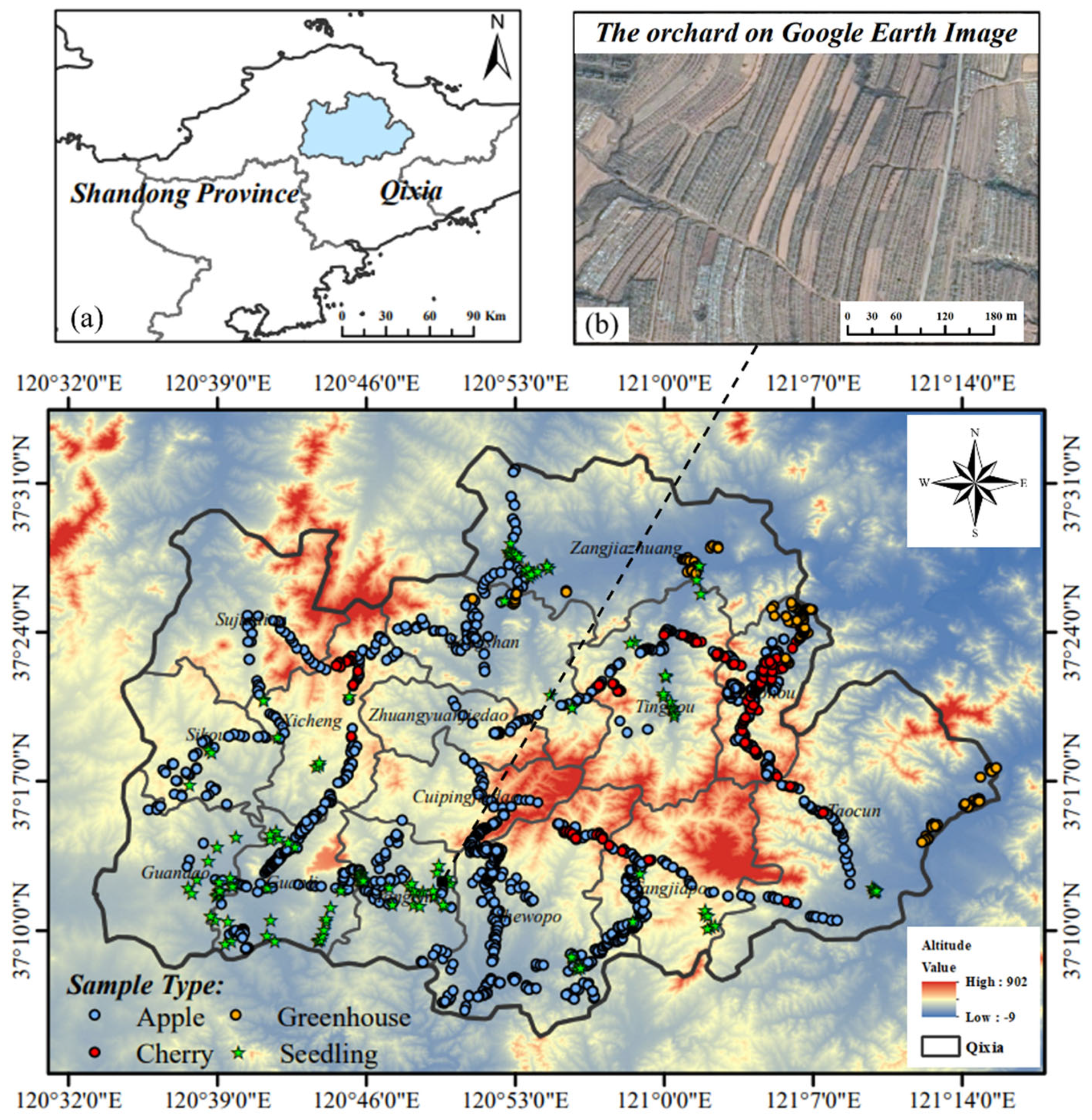
Figure 1. The location of the study area: the dot represents the location of the sampling point, and the background is DEM. (a) Shows the geographical location of the study area. (b) Shows the visual characteristics of the orchard on a Google Earth image.
Remotesensing 15 00175 g001
Figure 2. Crop phenological information and image acquisition time of regular time series.
Remotesensing 15 00175 g002
Figure 3. Grid division result. Points expanded into polygons.
Remotesensing 15 00175 g003
Figure 4. Irregular time series data information. Different colors represent the number of images in different months, and dots indicate that there are images selected in this period.
Remotesensing 15 00175 g004
Figure 5. Workflow of the method proposed in this paper.
Remotesensing 15 00175 g005
Figure 6. Schematic diagram of irregular time series.
Remotesensing 15 00175 g006
Figure 7. Classification flow chart based on 2DCNN.
Remotesensing 15 00175 g007
Figure 8. LSTM cell structure.
Remotesensing 15 00175 g008
Figure 9. The distribution map of farmland parcels in the study area using the proposed method. (A, B) are sub-regions of the study area.
Remotesensing 15 00175 g009
Figure 10. Statistical chart of land parcel information of different areas.
Remotesensing 15 00175 g010
Figure 11. Parcel extraction results: (a)–(c) are the sub-regions of the study area; the geographical location in this study is shown in (P1, P2, P3) in Figure 9; (a2) shows the extraction effect of terraced parcels; (b2) shows the extraction effect of seedling parcels; and (c2) shows the extraction effect of regular parcels and greenhouses.
Remotesensing 15 00175 g011aRemotesensing 15 00175 g011b
Figure 12. Accuracy evaluation of different experimental results. (a) Is the confusion matrix of the classification results with “irregular time series + 2DCNN”; (b) is the confusion matrix of the classification results with “regular time series + 2DCNN”; (c) is the confusion matrix of the classification results with “regular time series + LSTM”; (d) shows the overall accuracy of different grids.
Remotesensing 15 00175 g012
Figure 13. Parcel category filling results. (A)–(C) are sub-regions of the study area.
Remotesensing 15 00175 g013
Table 1. Specifications of Sentinel-2 images.
Data AttributeDescription
Product TypeLevel 2A
Pixel size10 m
Spectral BandsBandCentral wavelength(nm)Bandwidth (nm)
B2: Blue49065
B3: Green56035
B4: Red66530
B8: NIR842115
Table 2. Table of sample data.
Parcel TypeTrain DataValidation Data
Apple26,7286682
Seedling11,4482862
Cherry2632658
Greenhouse3044761
Table 3. Parcel type table.
Geographic AreaFarmland TypeFeatures
Plain AreaGreenhouse parcelsRegular shape, clear boundary, distributed in plain areas, and different from the surrounding crop background.
Regular parcelsPlain parcels, regular shape, clear boundaries, uniform internal texture, and uniform area.
Mountain AreaTerrace parcelsLong and narrow shape with uniform width, clear boundaries, uniform internal texture, and regular arrangement.
Slope parcelsFuzzy boundary, uniform internal texture, irregular shape, irregularly distributed on the hillside, and great difference in area.
Table 4. Evaluation of parcel extraction effect.
Accuracy Evaluation IndexRadius of Buffer
1 m2 m
Recall0.970.98
Precious0.890.94
F1-score0.930.96
IoU0.872
Table 5. Information obtained from different types of parcels.
Parcel TypeNumberArea (m2)
Apple orchard415,23379,9424,375.7 ( A a 1 )
Cherry orchard19,45523,766,845.11 ( A c 1 )
Seedling403131,212,521.33
Greenhouse411822,299.1387
Mixed parcel30,72442,699,347 ( A a 2 )
33,875,728 ( A c 2 )
Disclaimer/Publisher’s Note: The statements, opinions and data contained in all publications are solely those of the individual author(s) and contributor(s) and not of MDPI and/or the editor(s). MDPI and/or the editor(s) disclaim responsibility for any injury to people or property resulting from any ideas, methods, instructions or products referred to in the content.