Article

Accuracy of Rockfall Volume Reconstruction from Point Cloud Data—Evaluating the Influences of Data Quality and Filtering

1
Department of Geology and Geological Engineering, Colorado School of Mines, Golden, CO 80401, USA
2
BGC Engineering, Golden, CO 80401, USA
*
Author to whom correspondence should be addressed.
Remote Sens. 2023, 15(1), 165; https://doi.org/10.3390/rs15010165
Submission received: 9 November 2022 / Revised: 15 December 2022 / Accepted: 26 December 2022 / Published: 28 December 2022
(This article belongs to the Special Issue Remote Sensing in Engineering Geology - II)

Abstract

:
Rockfall processes are now commonly studied through monitoring campaigns using repeat lidar scanning. Accordingly, several recent studies have evaluated how the temporal resolution of data collection and various data-processing decisions can influence the apparent rockfall volumes estimated using typical rockfall database creation workflows. However, there is a lack of studies that consider how data quality and associated data-processing decisions influence rockfall volume estimation. In this work, we perform a series of tests based on an existing reference rockfall database from the Front Range of Colorado, USA, to isolate the influences of data resolution (point spacing), individual point precision, and the filter threshold applied to change results, on the volume estimates obtained for rockfalls. While the effects of individual point precision were found to be limited for typical levels of gaussian noise (standard deviation per coordinate direction ≤ 0.02 m), data resolution and change filter threshold were found to have systematic impacts on volume estimates, with the volume estimates for the smallest rockfalls decreasing substantially with increases in point spacing and change filter threshold. Because these factors disproportionately impact volume estimates for smaller rockfalls, when these factors change, the slope of the apparent power law that describes the relative frequency-volume distribution of rockfalls changes. Evidence is presented that suggests that this phenomenon can explain discrepancies between power law slopes presented in the literature based on studies focused on different scales of rockfall activity. Overall, this study demonstrates the impacts of raw data attributes on rockfall volume estimation and presents an additional effect that tends to bias rockfall frequency–magnitude power law relationships towards underestimation of the relative prevalence of small rockfalls.

1. Introduction

Rockfall is a hazard that is prominent in mountainous regions around the world. In addition to major catastrophic events that can represent significant safety hazards [1,2], smaller, more frequent rockfalls along transportation corridors can have negative economic impacts, including direct maintenance and repair costs, and indirect economic losses associated with delays caused by lane closures [3,4]. Accordingly, rockfall has been widely studied, both from a physical process perspective [5] and a risk management perspective [6]. In both cases, quantitative information with respect to rockfall size (volume) and their relative frequency can be useful [7].
Over the past decade, there has been a substantial increase in the application of lidar to rockfall characterization and monitoring through repeated scanning at various time intervals [8,9,10,11,12]. Photogrammetric methods have also been employed where lidar monitoring may be impractical or cost-prohibitive, with similar end goals [13,14,15]. The increasing volumes of collected data are motivating research in applying advanced computer vision techniques and machine learning for automatic measurement and interpretation [16,17,18,19,20]. While a lidar-based approach for rockfall activity characterization has several advantages over conventional approaches (e.g., visual inspection, manual mapping of ditch debris, etc.), arguably one of the most significant is the ability to keep three-dimensional (3D) records of rockfall shapes and develop associated quantitative volume estimates [21,22]. One risk of developing such quantitative volume estimates, however, is the potential to develop a sense of overconfidence in the accuracy of the results obtained. Most recently, there has been increased scrutiny of factors unrelated to the physical rockfall processes being monitored and their influences on the accuracy of lidar-derived volume estimates. Perhaps the most notable and well-established finding in this regard is that the monitoring frequency used can impact the apparent relative proportions of small and large rockfalls [23]; specifically, spatial grouping of small rockfalls that occur between successive scan dates can result in underestimation of the number of small rockfalls and overestimation of the number of large rockfalls. The degree to which this issue manifests depends both on the spatiotemporal clustering patterns of rockfall at a given site and the specific monitoring interval (s) considered [11,23,24].
Other studies have focused specifically on how data-processing decisions influence rockfall volume estimates derived from lidar change detection results. DiFrancesco et al. [25] considered the influence of multi-scale cloud-to-cloud comparison (M3C2) projection diameter on lidar-derived volume estimates and found that although the volumes of the smallest recorded rockfalls were notably influenced, the effects on rockfalls in the linear portion of the magnitude–cumulative–frequency (MCF) curve were negligible. Winiwarter et al. [26] proposed a modified change detection algorithm based on M3C2 and demonstrated that it produced significantly different total movement volume estimates from M3C2, although they did not present results regarding the influence on individual rockfall volume estimates. When using alpha shape surface reconstruction, Carrea et al. [27] demonstrated the influence of selected alpha radius value on the obtained rockfall distribution. To develop a rational, reproducible approach to select the alpha radius, Bonneau et al. [28] proposed the alphaSolid method which has since become increasingly accepted [22,24,29]; specifically, for each set of points defining a rockfall, this method automatically produces a volume estimation using the minimum alpha radius that results in a watertight manifold surface with correct topology. More recently, DiFrancesco et al. [22] compared volume estimates produced by alphaSolid with those obtained using a the more sophisticated Power Crust surface reconstruction algorithm [30] and found that while alphaSolid systematically overestimated by over 50% in some cases, the degree of overestimation relative to Power Crust was relatively consistent for rockfalls of varying sizes, meaning the slope of the derived MCF curve was consistent between the methods.
While the work of DiFrancesco et al. [22] provides valuable insights into the influences of surface reconstruction methods on volume estimation given a certain set of lidar-derived rockfall data points, we are not aware of any studies that evaluate the influence of lidar data quality attributes, such as density and precision, on rockfall volume estimates. This is of great interest for rockfall studies, because point cloud data are collected under a wide range of quality conditions dictated by budget, accessibility, study goals, and other site-specific considerations. We hypothesize that data resolution (controlled by point spacing), individual point positional precision, and overall change detection uncertainty may influence the volume estimates obtained using common surface reconstruction techniques, perhaps as much as or even more so than the specific reconstruction techniques themselves.
In this study, we use an existing rockfall database [31] as a starting point and apply various perturbations to the point clouds that define individual rockfalls in the database to assess the effects of different data quality attributes. Specifically, we evaluate the influences of data resolution (i.e., point spacing/number of points), individual point precision, and parameters utilized in the process of extracting rockfall point clusters from raw change detection results; in this last case, we note that the parameters utilized are determined based on change detection uncertainty, which in turn depends largely on the quality of the raw data sets used for change detection. While the specific quantitative results obtained are only applicable for the specific site and rockfall surface reconstruction method evaluated, we argue that the overall trends observed should be more broadly applicable. Additionally, this study demonstrates an analysis framework that could be applied to data from other slopes in future studies.

2. Materials and Methods

2.1. Reference Rockfall Database

The reference rockfall database used for this study was developed for a slope approximately 6 km East of Idaho Springs, Colorado, USA, bordering the westbound lane of Interstate Highway 70 (I-70). The slope is a sub-vertical (approximately 72°) cut in biotite gneiss, with prominent foliation and three major fracture sets (see Figure 1). The unit is situated in the uplifted basement rock of the Colorado Front Range, with a high density of regional faults and felsic dike intrusions. The slope presents a risk to motorists due to the relatively narrow corridor and ditch, combined with a high traffic volume. The largest, most disruptive rockfall events in recent records have been triggered by torrential summer storms, conditioned by freeze–thaw cycles in the preceding winter months. While vehicle impacts are rare, rockfalls regularly cause closures of the highway for scaling, clearing, and mitigation. In 2022, a large 30–40 m3 marginally stable block was pre-emptively mitigated using rock bolts and wire mesh [32,33], but otherwise there are no permanent control measures in place to reduce rockfall risk.
The total monitored area is approximately 14,000 m2, and the database was constructed using repeat terrestrial lidar scanning data collected between 11 February 2016 and 31 August 2021 at a typical data collection frequency of every 2 to 3 weeks, although in some cases longer periods of time elapsed between scans (most notably a major data gap from 10 November 2016 to 26 October 2017). The point spacing of the slope point clouds is approximately 2 cm.
To produce a rockfall database from the raw lidar data collected, standard processing steps were followed [11,25,34,35] using a workflow and code originally developed by Schovanec et al. [36] and adapted for application to the Floyd Hill site as documented in detail by Malsam et al. [24,31]:
  • Alignment: Individual scans from four separate scanning positions were placed in a common coordinate system (no absolute georeferencing) using a two-step coarse-fine alignment procedure.
  • Classification: A manually developed static mask was used to identify and remove non-bedrock points from the point cloud. The mask is a point cloud with one of two class labels applied to each point on the slope: “rock” and “other”. Rock represents bare rock slope points used to compute change detection, and “other” indicates regions of vegetation, roads, guard rails, and other objects not relevant to change detection. For each point in the aligned point cloud, the nearest neighbor point was found from the mask point cloud and its label was copied over to the aligned cloud. Then, all points labeled as “other” were removed.
  • Change Detection: M3C2 was used to compare each pair of point clouds from successive scan dates.
  • Clustering: A change filter threshold was used to remove points with calculated change values below a specified value; the remaining points were then clustered using the DBSCAN algorithm [37].
  • Cluster Filtering: Many of the clusters produced by the clustering process represent regions of spurious (i.e., non-rock) change, typically associated with locally high error or small vegetation not removed in the “Classification” step. To determine which clusters are representative of rockfall, a random forest classifier tuned to produce almost no false negatives (i.e., no missed rockfalls) was applied to remove a portion of the spurious clusters, and the remaining clusters were manually classified as “rockfall” or “clutter” based on visual inspection.
  • Volume Calculation: Volumes for all clusters manually classified as “rockfall” were estimated using the alphaSolid approach of Bonneau et al. [28].
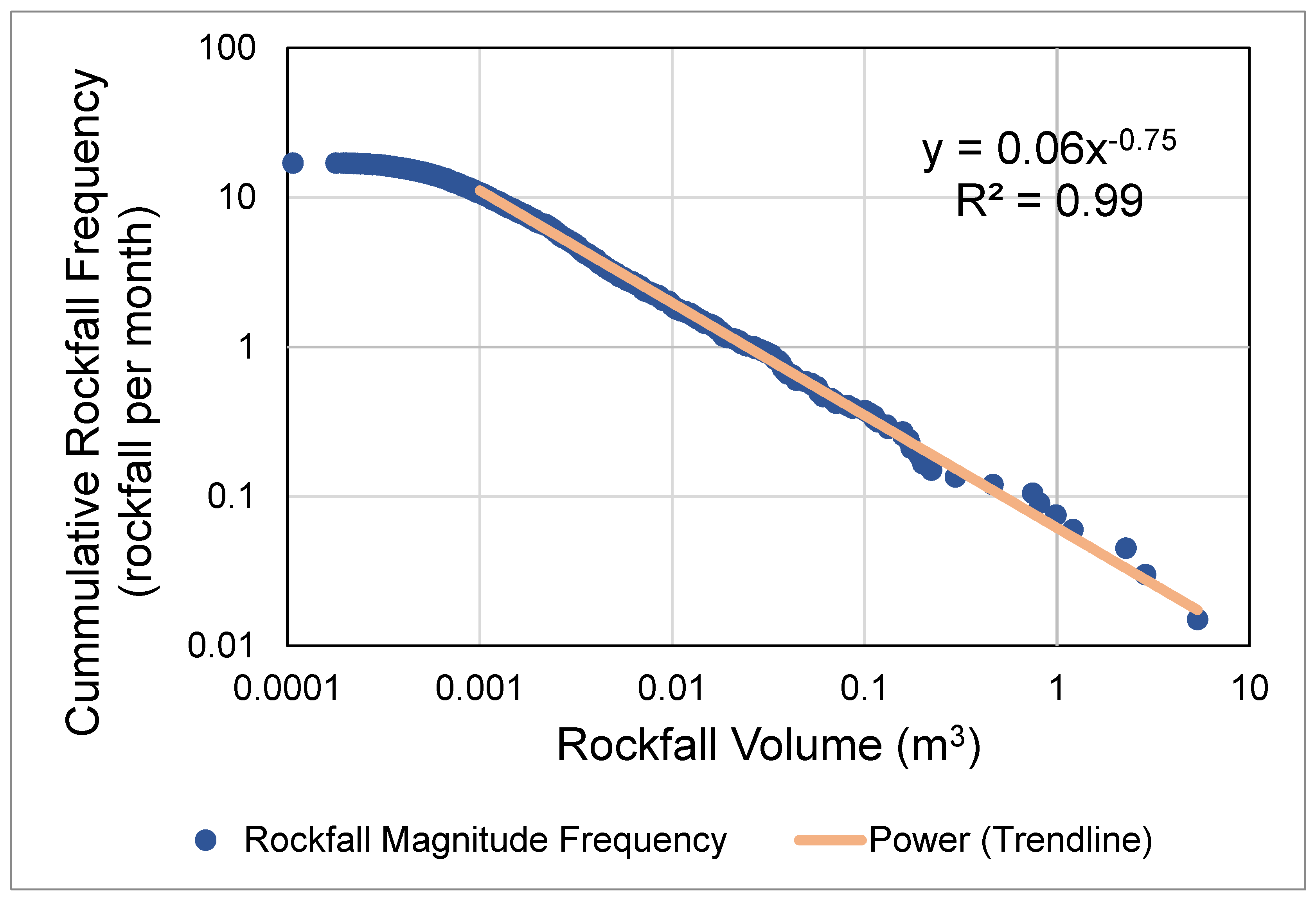
The final rockfall database produced by Malsam [31] and used as the basis of this study is visually represented as an MCF curve in Figure 2. Most of the recorded rockfalls were small, with only four being larger than 1 m3 (per the alphaSolid volume estimates). The power law trend (Equation (1)) observed above a specific volume threshold is typical for rockfall and has been documented for a large number of slopes worldwide [38,39]:
F ( V ) = a V b
where V represents rockfall volume, a is a constant dependent on the total level of rockfall activity at a given slope, b is a constant that depends on the relative proportions of large and small rockfalls, and F(V) is the number of rockfalls with volume greater than or equal to V.
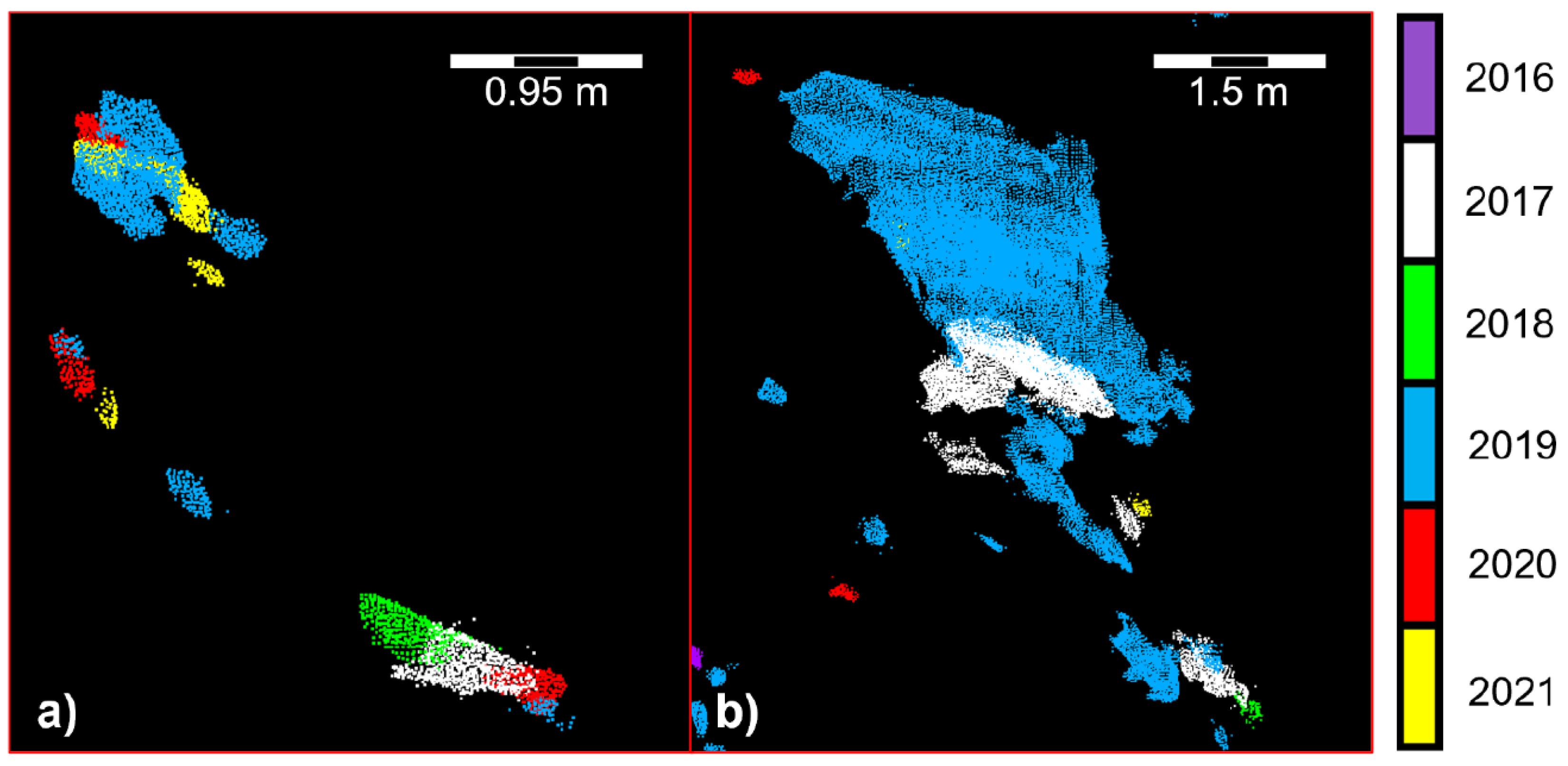
Most of the rockfalls at the site, and in particular the relatively large ones, tend to exhibit some elongation along the foliation (see Figure 3). While the rockfalls at the site tend not to be highly spatially clustered [24], there are cases where release of one block has been observed to destabilize an adjacent part of the rockmass.

2.2. Analysis Methods

Three separate analyses are presented in this study:
  • Resolution Analysis—quantification of the influence of lidar point spacing on rockfall volume estimates by downsampling relative to high resolution reference clouds;
  • Precision Analysis—quantification of the influence of individual point precision on rockfall volume estimates by addition of gaussian noise to reference clouds;
  • Filter Threshold Analysis—quantification of the influence of the filtering and clustering process on rockfall volume estimates.
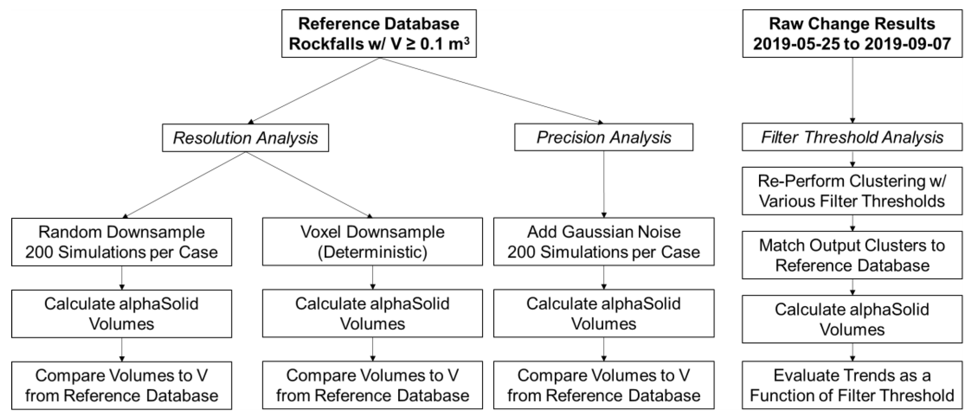
A flowchart that summarizes the methods applied for each of these analyses is presented in Figure 4. The following sub-sections describe the specific analysis procedures in detail.

2.2.1. Assessment of Point Spacing Influence

Downsampling was conducted using the pcdownsample function in MATLAB with two different approaches: random and voxel downsampling. Because of the stochastic nature of the random downsampling approach, each degree of downsampling (5%, 10%, 20%, 30%, 50%, 70%) was repeated 200 times and mean values were recorded for the resulting volumes. In the case of voxel downsampling, the averaging that occurs within each voxel has the effect of smoothing the point cloud, so although this method has the advantage of providing a single deterministic result for a given level of downsampling, the precision of the points in the downsampled cloud is effectively improved relative to the actual raw lidar data. Voxel edge lengths (2 cm, 3 cm, 4 cm, 5 cm, 7 cm, 10 cm, 15 cm, 20 cm) were selected to roughly cover the same range of average point spacing produced by the random downsampling procedure.
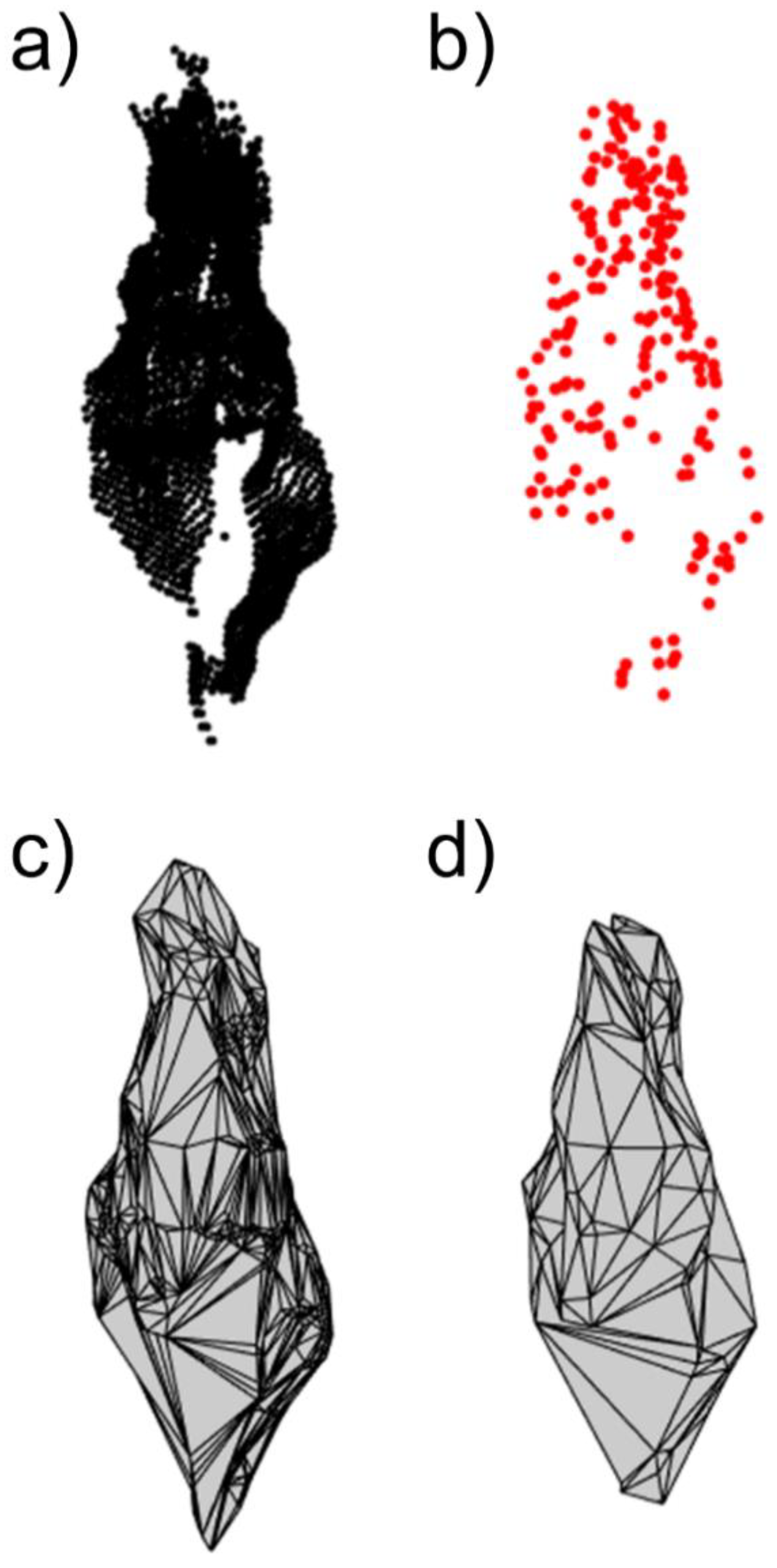
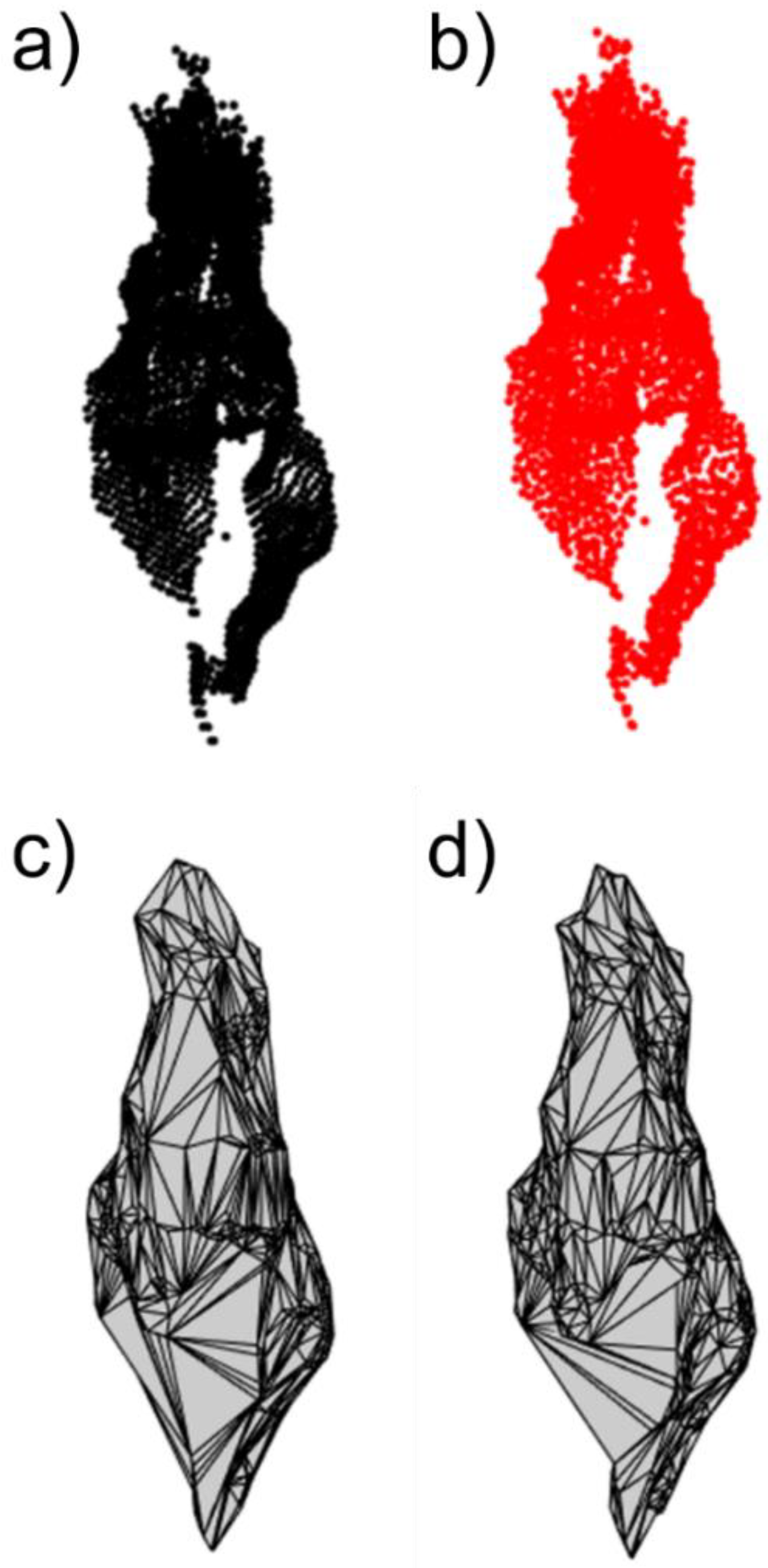
The downsampling procedure was only applied to rockfalls in the reference database with volumes (Vreference) greater than or equal to 0.1 m3 to ensure each rockfall considered would be defined by a sufficiently large number of points to allow for downsampling as specified above; a total of 27 such rockfalls were used for this analysis. After downsampling, the alphaSolid method [28] was applied to estimate volumes for each of the downsampled point clouds, and these volumes were then compared to the corresponding volume values for the original rockfall point clouds from the reference database, typically by calculation of a ratio of volumes (i.e., Vdownsampled/Vreference). Figure 5 illustrates a representative rockfall before and after downsampling, as well as the resulting surface mesh reconstructions produced by the alphaSolid process.
Following volume calculation, magnitude–cumulative–frequency (MCF) plots were produced for each of the downsampling cases. In the voxel cases, the MCF curves were developed based on the deterministic downsampled results for each rockfall. In the random downsampling cases, the MCF curves were developed using the mean volume values from the 200 realizations for each rockfall. Power laws were fit to all volumes in both cases using a least-squares regression, as the initial volume cutoff applied for the analysis (Vreference ≥ 0.1 m3) ensured that all volumes were past the power-law rollover cutoff volume (identified as 0.001 m3 for the reference database by [31]). Note that the MCF curve represents an approximation of the complementary cumulative distribution function (CCDF) of the rockfall inventory [40], and the power law slope values produced are therefore close to those associated with the true CCDF [38].

2.2.2. Assessment of Point Precision Influence

The influence of point precision on rockfall volume estimation was evaluated for the same subset of reference rockfalls as considered in the resolution analysis (Vreference ≥ 0.1 m3). In this case, each reference point cloud had gaussian noise added to each of the three co-ordinates (x,y,z) of each point. The standard deviation of the noise was varied (0.0025 m, 0.005 m, 0.010 m, 0.015 m, 0.020 m, 0.050 m), and the mean was held constant at zero. For each initial rockfall point cloud and noise standard deviation, 200 point clouds with added noise were generated and mean values were recorded for the resulting volumes.
After the addition of random noise, the volume of each new point cloud was estimated using the alphaSolid method [28], and these volumes were then compared to the corresponding volume values for the original rockfall point clouds from the reference database, typically by calculation of a ratio of volumes (i.e., Vadded-noise/Vreference). Figure 6 illustrates a representative rockfall before and after the addition of random noise, as well as the resulting surface mesh reconstructions produced by the alphaSolid process.

2.2.3. Assessment of Change Filter Threshold Influence

The change filter threshold (t) is the value of change below which points are removed prior to grouping of points into change clusters. This filter is applied to ensure that individual regions of change potentially associated with rockfall are spatially distinct from one another before the application of a clustering algorithm. Additionally, by using a sufficiently large value of t, typically on the order of the limit of detection, the number of spurious (i.e., non-rockfall) clusters identified can be minimized.
Evaluating the influence of change filter threshold required re-running the clustering and cluster filtering steps of the rockfall database development workflow for each filter threshold value. Because this represents a non-trivial computational and manual task, a subset of 10 change detection results derived from 11 scans taken between 25 May 2019 and 7 September 2019 were used as the basis for re-constructing rockfall clusters with different change filter thresholds (t = 0.015 m, t = 0.020 m, t = 0.030 m, t = 0.050 m, and t = 0.100 m). This range of dates was selected as it corresponded to a period of relatively high rockfall activity, including multiple large (Vreference > 1 m3) rockfall events. All rockfalls detected during this range of dates were considered regardless of volume.
For each change detection result and a given filter threshold case, points with change values below the filter threshold were removed. Then, the remaining points were clustered using the DBSCAN algorithm [37]. Although we found that the DBSCAN parameters used in the construction of the reference database (Eps = 0.1 m, MinPts = 16) produced clusters representative of actual visually assessed rockfall shapes for the t = 0.020 m and t = 0.030 m cases, the smallest (t = 0.015 m) and two largest (t = 0.050 m and t = 0.100 m) filter threshold cases encountered different issues. In the t = 0.015 m case, the Eps = 0.1 m value was found to be too large, as it resulted in the algorithm extending rockfall clusters to include nearby noisy points above the (relatively permissive) t = 0.015 m filter threshold. In the case of the two largest filter thresholds, the Eps = 0.1 m value was found to be too small, as the remaining unfiltered points on the front and back faces of several rockfalls were over 0.1 m apart, leading to the creation of several clusters containing only one face of a given rockfall. In both cases, using a fixed Eps value for a large range of t had a confounding influence on computed rockfall volumes.
With this in mind, it was determined that variable Eps values should be used for the different values of t. This reflects the reality that in different practical application cases with different levels of change detection uncertainty and different filter thresholds, Eps values would be tuned to account for site-specific and data-specific conditions [11,35,37]. Accordingly, although results are presented in terms of the influence of t, this analysis effectively considers the combined effects of t and Eps on rockfall volume estimation as a proxy for the influence of change uncertainty on rockfall estimation. In other words, in practice, the change uncertainty at a given site constrains the t value used, and the Eps value used for clustering is selected to produce the best clustering performance for a given filtered point cloud. The Eps values used for each filter threshold (t) case considered are summarized in Table 1.
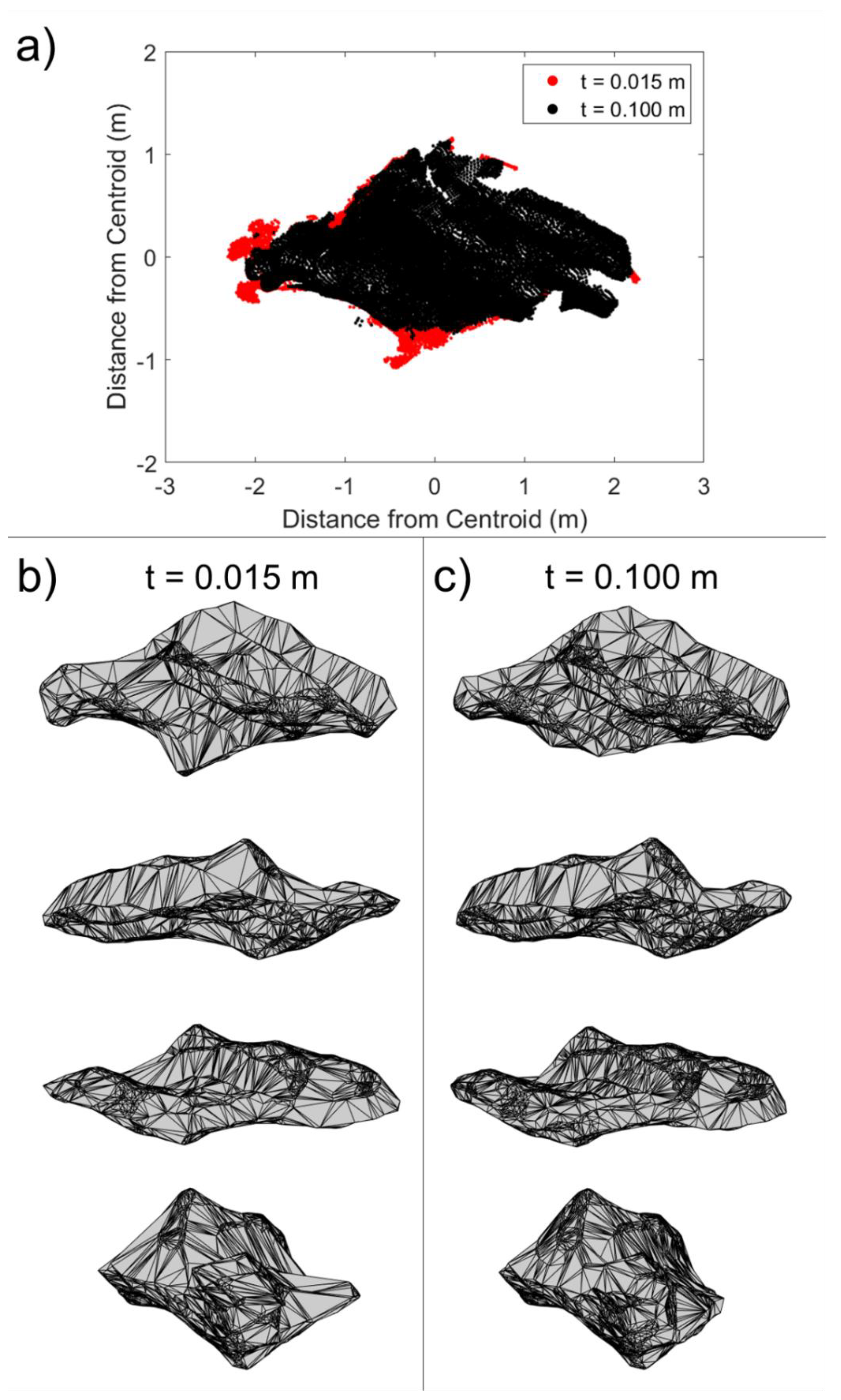
Figure 7 presents an example of how filter threshold can influence the estimated volume for a given rockfall cluster. Specifically, the t = 0.015 m change filter removes fewer points from the point cloud prior to clustering than for t = 0.1 m, resulting in a larger number of points being included in the cluster, and ultimately a larger volume estimate.
For a given data set, the clusters output by DBSCAN need to be filtered to separate clusters representing true rockfalls from “clutter” clusters [36]. An example illustrates the necessity of this filtering: in the t = 0.015 m case for the 18 August 2019 to 31 August 2019 scan interval alone, 1514 clusters were produced despite only three manually verified rockfalls having been identified. Even with the assistance of a potentially error-prone Random Forest classifier, filtering many iterations of clustering with different parameters across 10 time intervals would be impractical.
As an alternative to manually filtering clusters, we used the reference database of already-identified rockfalls to locate true rockfalls in each experimental condition. Specifically, for each of the rockfalls in the reference database, the single nearest neighbor cluster from the corresponding scan interval for a given value of t was identified; if this nearest neighbor cluster was found to have a centroid within 0.5 m of the centroid of the reference rockfall cluster, it was flagged as a candidate cluster and assigned the same identification number as the corresponding rockfall cluster. The 0.5 m distance threshold was selected to be relatively permissive as a first round of filtering. As a result, not all candidate clusters ultimately were found to be representative of actual rockfall clusters representing the same rockfall identified in the reference database. Spot checking showed that in some cases, the candidate cluster was found to correspond to a nearby clutter cluster (i.e., when the actual rockfall was not detected for the given combination of t & Eps considered). In addition to the issue of identification of incorrect clusters, in some cases, the resulting clusters represented a partial match with a rockfall but did not accurately reflect the rockfall geometry. For example, some candidate clusters were found to include both rockfall points and nearby noise points, or in rare cases, the initial match cluster was missing one face of the rockfall cluster (despite the increase Eps values for the largest t cases).
With this in mind, an additional filtering step to remove spurious matches and clusters including non-rockfall points or missing one side of a rockfall was performed. This filtering step considered the centroid distance between a given candidate cluster and the corresponding reference rockfall cluster (dcentroid) relative to both the principal axis length of the reference rockfall cluster (lreference) and the calculated candidate cluster volume (determined using alphaSolid; Vcandidate) as well as the ratio between the number of points in the candidate cluster and the corresponding reference cluster (ncandidate/nreference). The ncandidate/nreference criterion was not applied to the t = 0.100 m clusters, as these clusters regularly contained much smaller numbers of points than their corresponding reference clusters. Ultimately, clusters were retained if they met three criteria:
  • dcentroid/lreference < 0.2;
  • dcentroid/Vcandidate < 100 m−2;
  • 0.25 < ncandidate/nreference < 2 OR t = 0.100 m.
In cases where a cluster contained extra non-rockfall points or one face of the rockfall was missing, the resulting movement of the candidate cluster centroid relative to reference cluster centroid was observed to be sufficiently large to be detected by the above criteria.
The total numbers of initial matches and final filtered rockfall clusters for each filter threshold case are summarized in Table 2; as a point of comparison, the total number of rockfalls in the reference database over the time period considered is 194. The decreased number of candidate clusters and final rockfall matches with increasing t is reflective of the decreased ability to detect relatively small rockfalls when using a restrictive change filter threshold. For example, for t = 0.100 m, 24 out of 27 of rockfalls with Vreference ≥ 0.01 m3 were detected, whereas only 4 out of 167 rockfalls with Vreference < 0.01 m3 were detected.
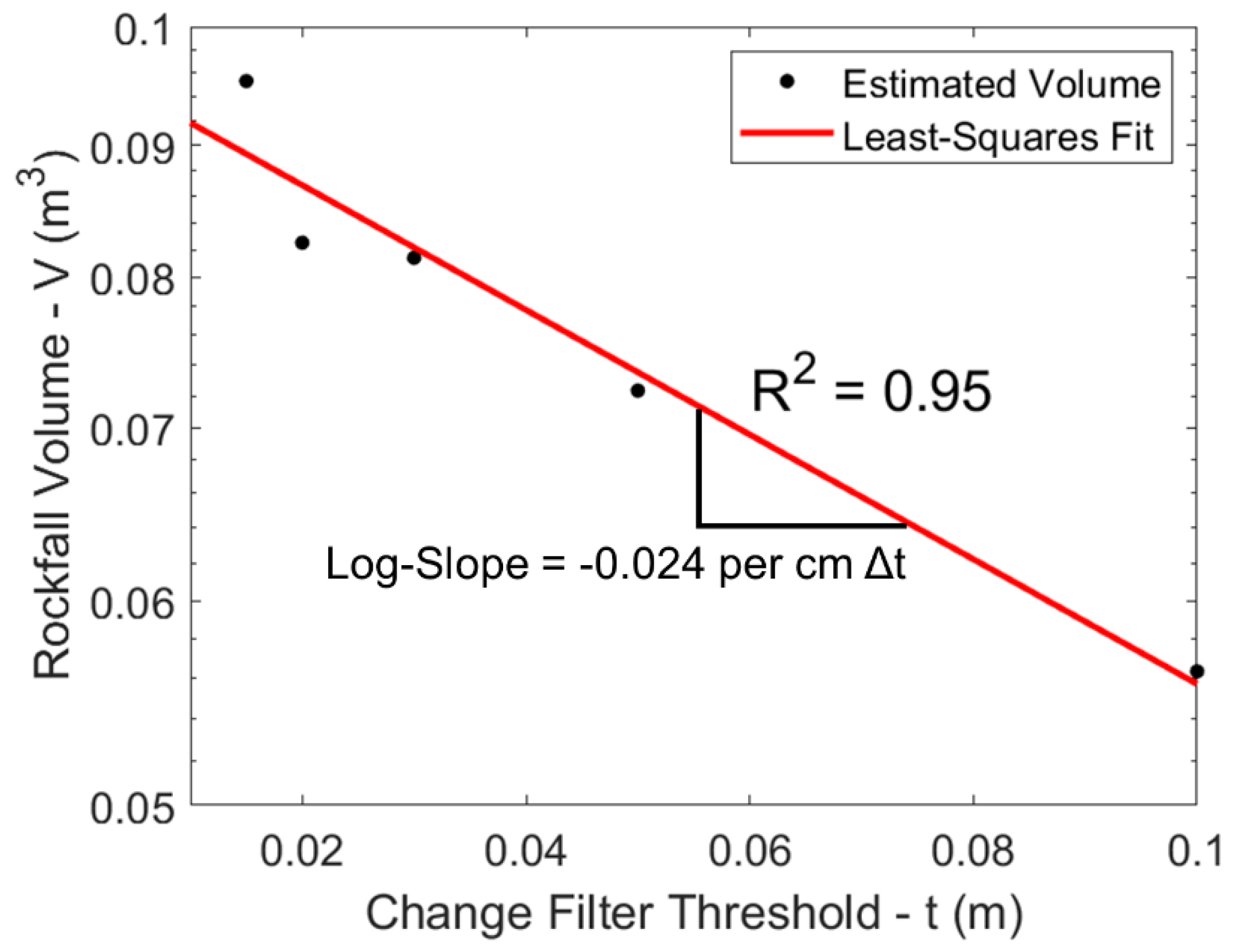
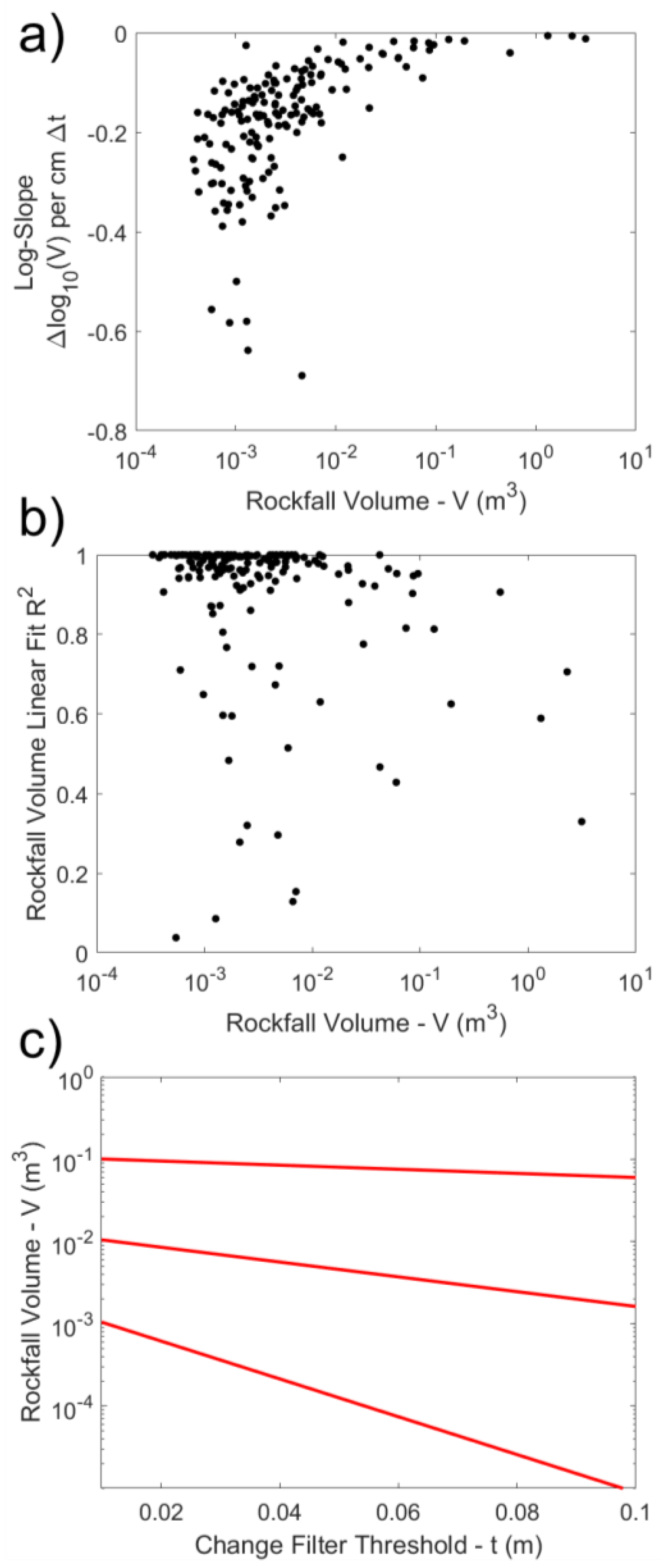
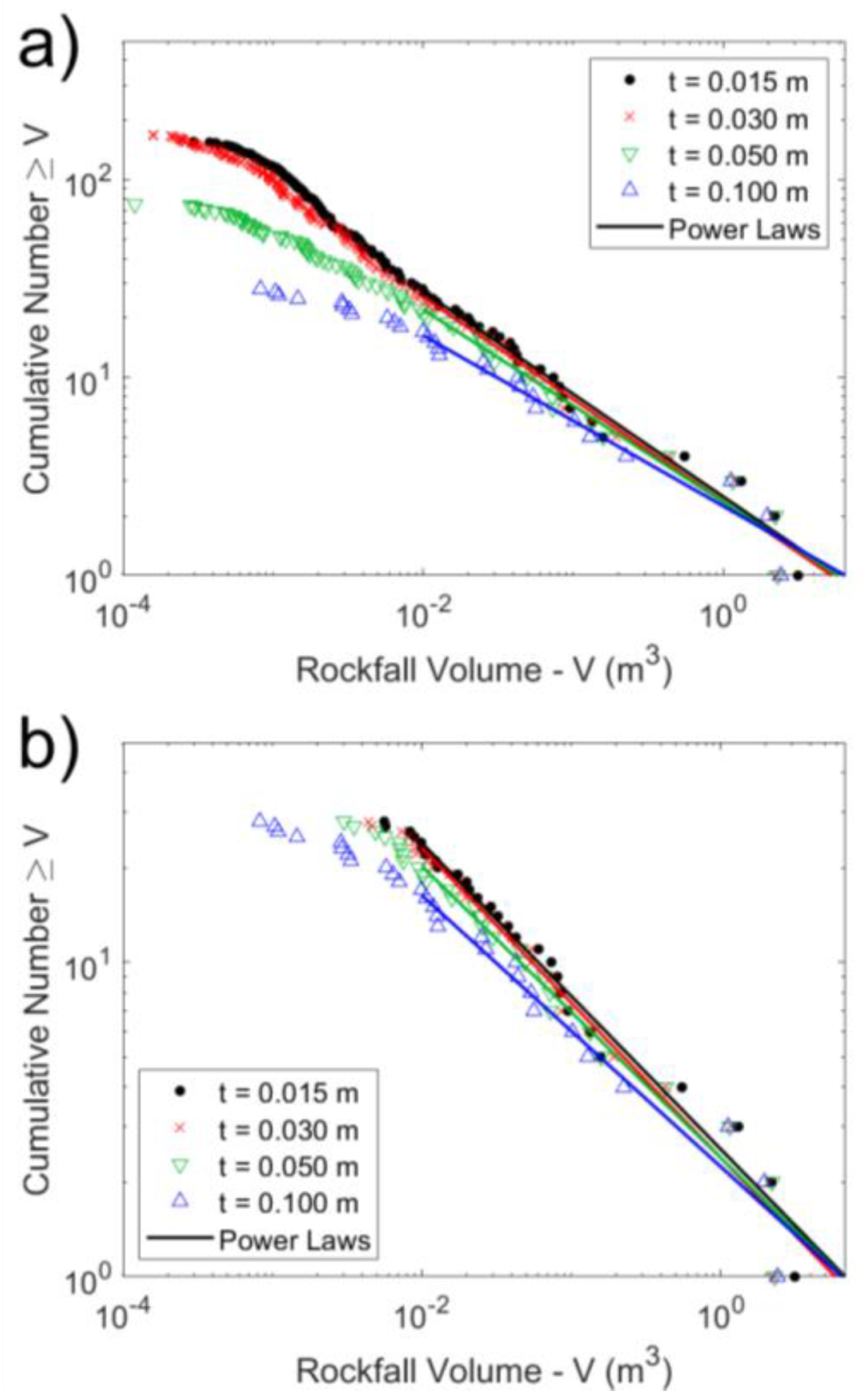
When evaluating the influence of t on estimated rockfall volume for a given reference rockfall, it was found that in most cases the logarithm of the estimated volume decreased approximately linearly as a function of t. Accordingly, for each reference rockfall, a linear regression was performed considering successfully matched rockfall clusters for each of the filter threshold (t) cases with t as the independent variable and the logarithm of the estimated volume as the dependent variable (see Figure 8). MCF curves were also created for each of the filter threshold cases to visualize the influences of the filtering and clustering procedure on the relative distribution of rockfall volumes. Additional MCF curves were developed for each case considering only the rockfalls for which a valid match to the reference database was identified for all filter threshold cases; this effectively isolates the effect of the change filtering and clustering on the volume reconstruction process due to inclusion of different points, removing the influence of rockfalls being entirely missed for some values of t (per Table 2). In both cases, power laws were fit to volumes with V ≥ 0.01 m3, which was visually assessed to ensure a linear trend in all cases considered.
We acknowledge that the specific quantitative results obtained from this analysis will depend to a certain extent on the filters applied to remove spurious clusters after the initial candidate cluster identification step. However, we note that cluster filtering procedures applied in the literature vary significantly from study to study [25,36,41], and there is no specific best practice to be applied, except perhaps manual verification, which was deemed impractical in this case and is not without error. Accordingly, the results obtained should be viewed with a focus on the overall trends identified, which are robust to minor changes in cluster filtering.

3. Results

3.1. Point Spacing Influence

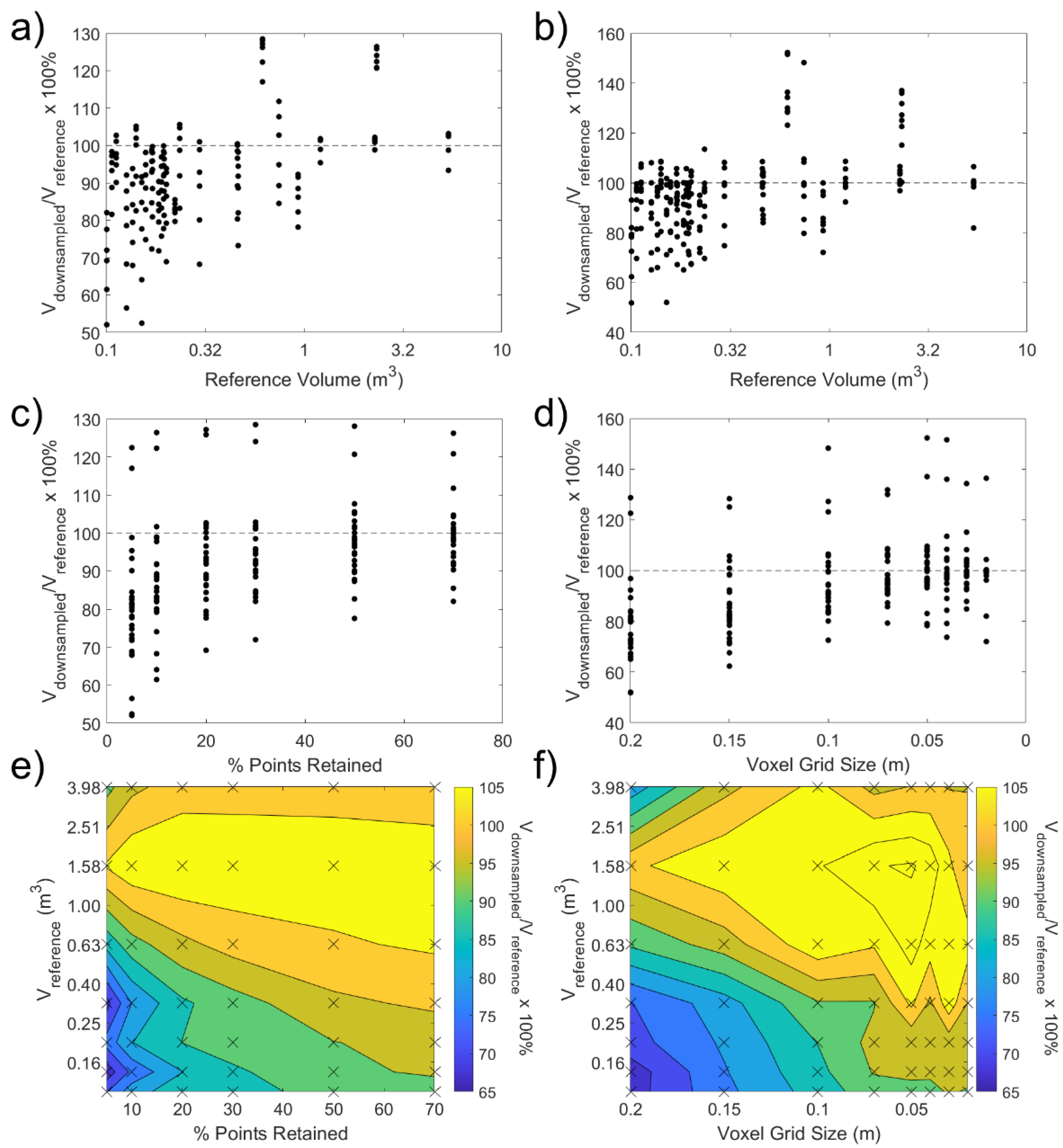
The results of the point spacing analysis are summarized in Figure 9, which shows trends in estimated rockfall volume (relative to the volume from the reference database) as a function of reference volume and degree of downsampling. Note that Figure 9a,b include all downsampling cases, and Figure 9c,d include all rockfall volumes. The interaction between the degree of downsampling and reference volume is represented in Figure 9e,f, where the average volume values calculated using an irregular set of bins of reference volume values for each level of downsampling are presented in the form of contour plots.
The results show that the main (and most consistent) effect of downsampling is to decrease the volume estimate produced by alphaSolid, and that this effect is most pronounced both for smaller volumes and for higher degrees of downsampling. The results are consistent for both the random downsampling and voxel downsampling cases.
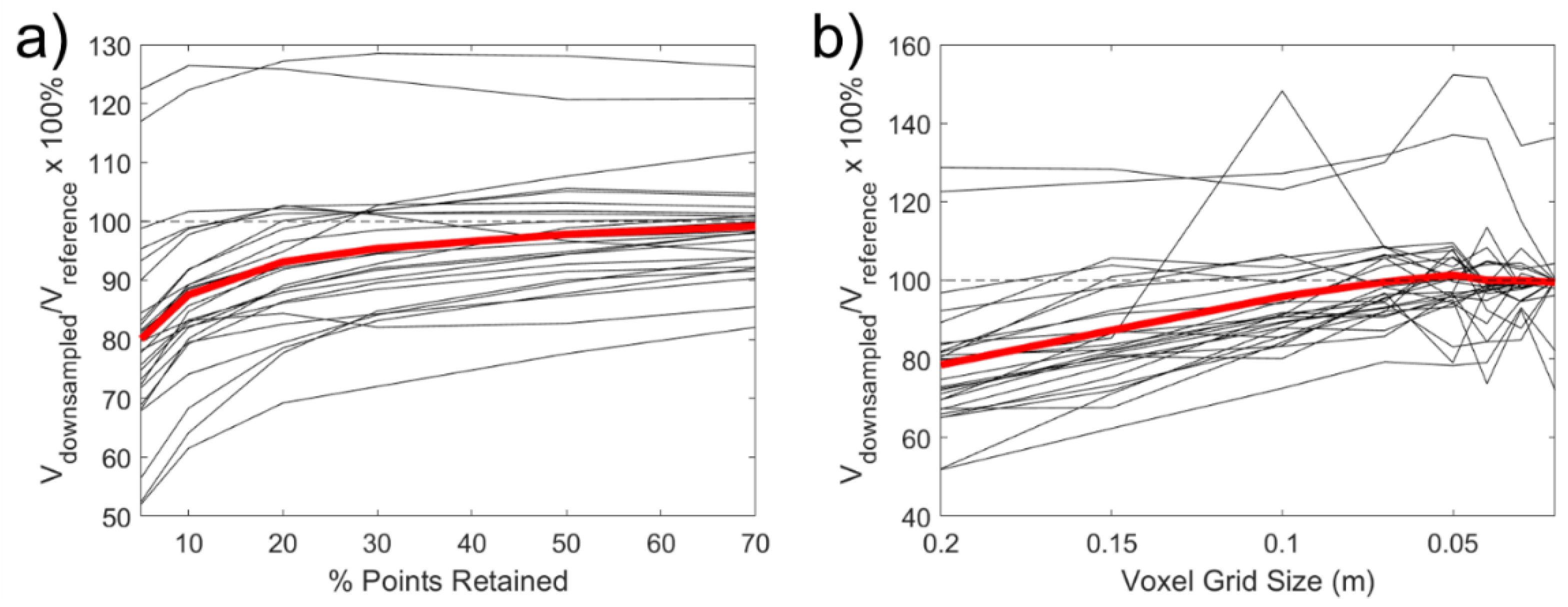
To allow the trends in volume estimates as a function of downsampling for each individual rockfall to be more clearly visualized, the results Figure 9c,d are replotted in Figure 10 with lines connecting the points representing each individual rockfall and the average across all rockfalls at each downsampling level shown in red.
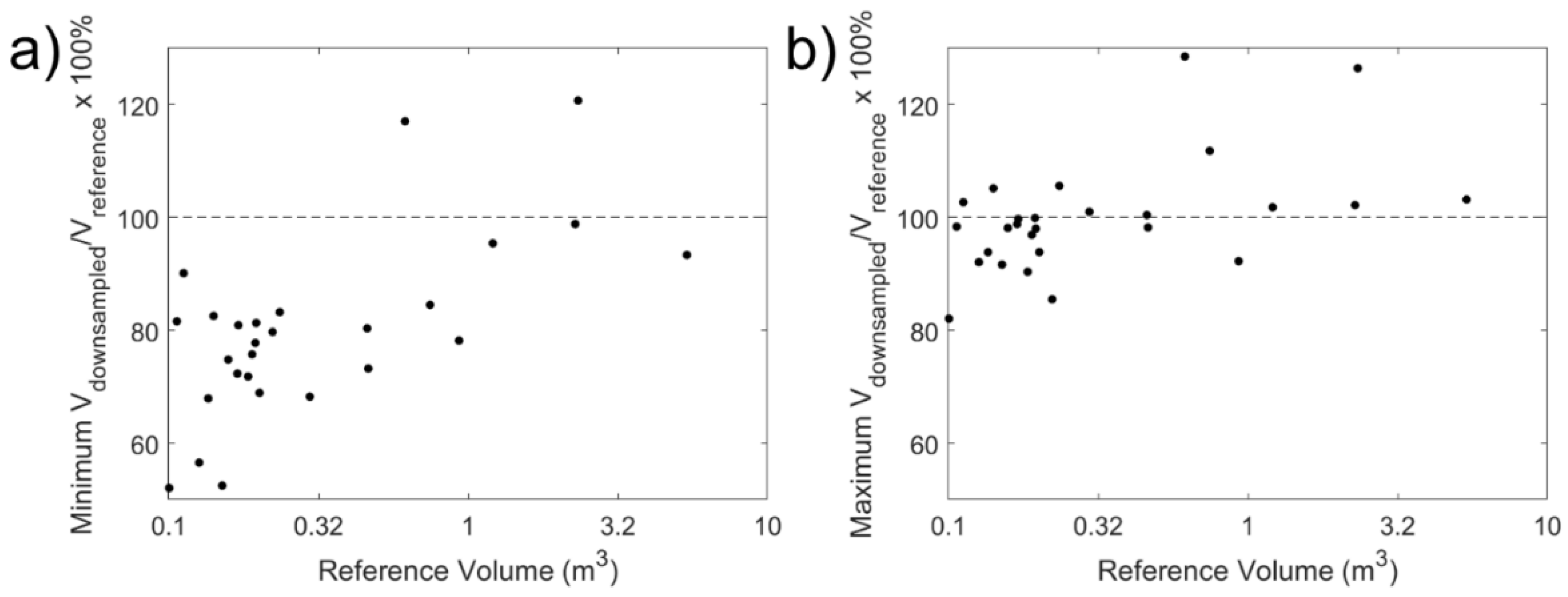
While Figure 9 and Figure 10 present results based on the average volume results across 200 simulations in the random downsampling case, Figure 11 presents the corresponding minimum and maximum volumes for each reference rockfall in the database. These results illustrate that, depending on the geometry of the specific rockfall point cloud considered, increased point spacing can, in extreme cases, lead to decreases in estimated volume by up to nearly 50%. However, the clustering of maximum volumes around the Vreference suggests that the specific changes in volume estimates can be highly dependent on exactly how removed points are spatially distributed, particularly for smaller volumes.
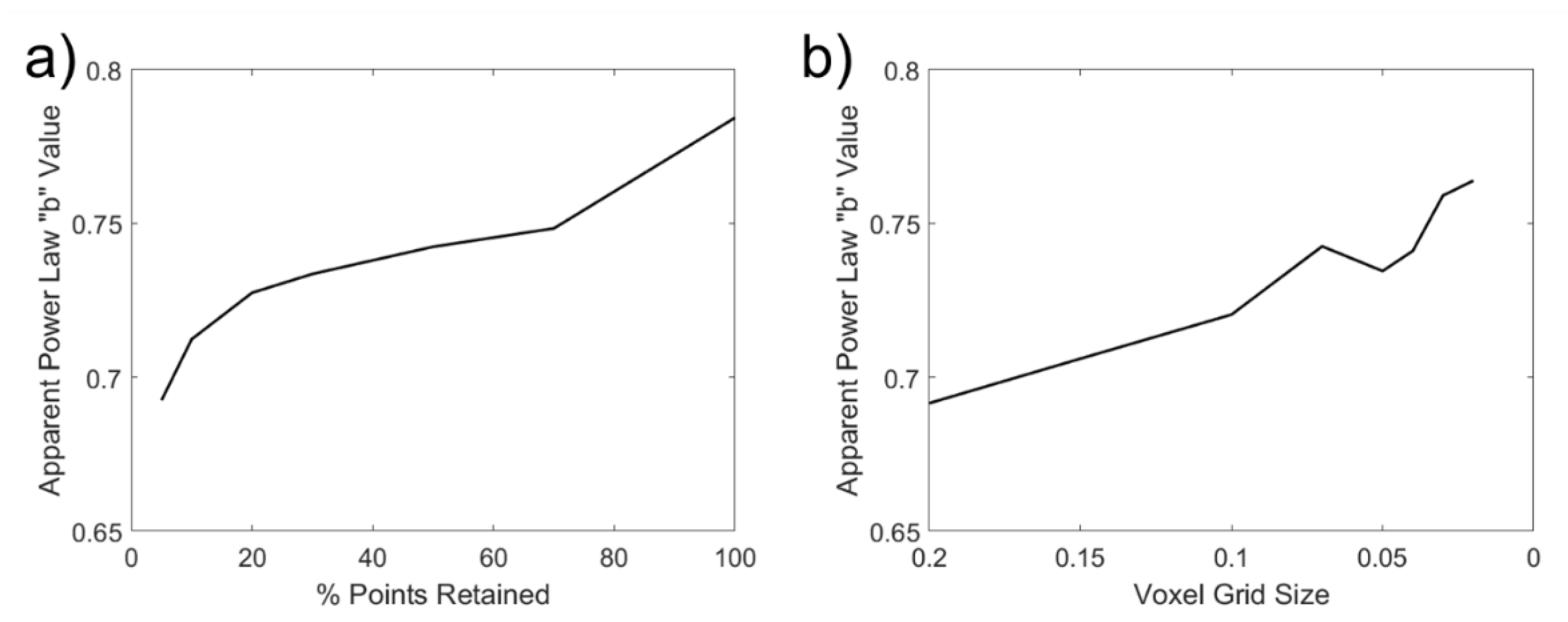
The fact that the influence of downsampling shows a non-uniform trend as a function of volume suggests that changes in the relative density of points defining a given rockfall has the potential to affect the relative volume trends of the MCF curve. This is confirmed by the results in Figure 12 for both the random and voxel downsampling cases. Figure 13 shows how the power law “b” parameter values (see Equation (1)) corresponding to the fits in Figure 12 vary depending on the degree of downsampling considered.

3.2. Point Precision Influence

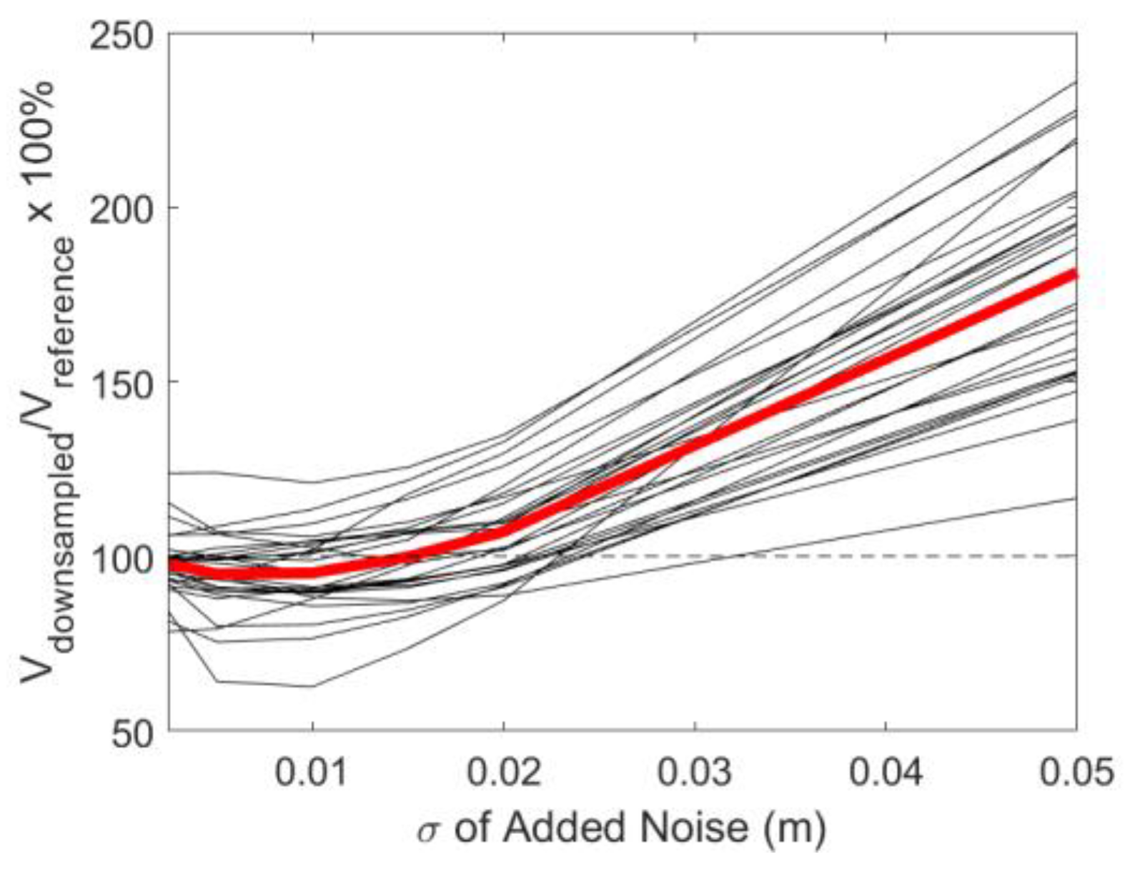
Figure 14 shows trends in average estimated rockfall volume as a function of the degree of random noise added to each point for each rockfall cluster. Although the specific influence of added noise varies depending on the rockfall considered, over the range of noise levels considered, the influence of added noise on rockfall volume estimates is limited. The general increasing trend beyond 0.01 m of added noise reflects the fact that for higher levels of noise, small numbers of outlier points can increase the alpha radius necessary for the alphaSolid algorithm to produce a watertight manifold mesh, leading to volume estimate increases.

3.3. Change Filter Threshold Influence

The linear regression results for the trends in estimated volume as a function of change filter threshold (t) for each individual rockfall cluster are presented in Figure 15. Figure 15a shows that the influence of t on volume estimates is proportionally larger for small rockfalls, even if it is larger in an absolute sense for large rockfalls. Additionally, Figure 15b illustrates that the (log-)linear trend in estimated volume as a function of t tends to be more consistent for smaller volumes (Figure 15b). Figure 15c presents representative examples of how the trend displayed in Figure 15a corresponds to changes in rockfall volume estimates as a function of t for rockfalls of different sizes.
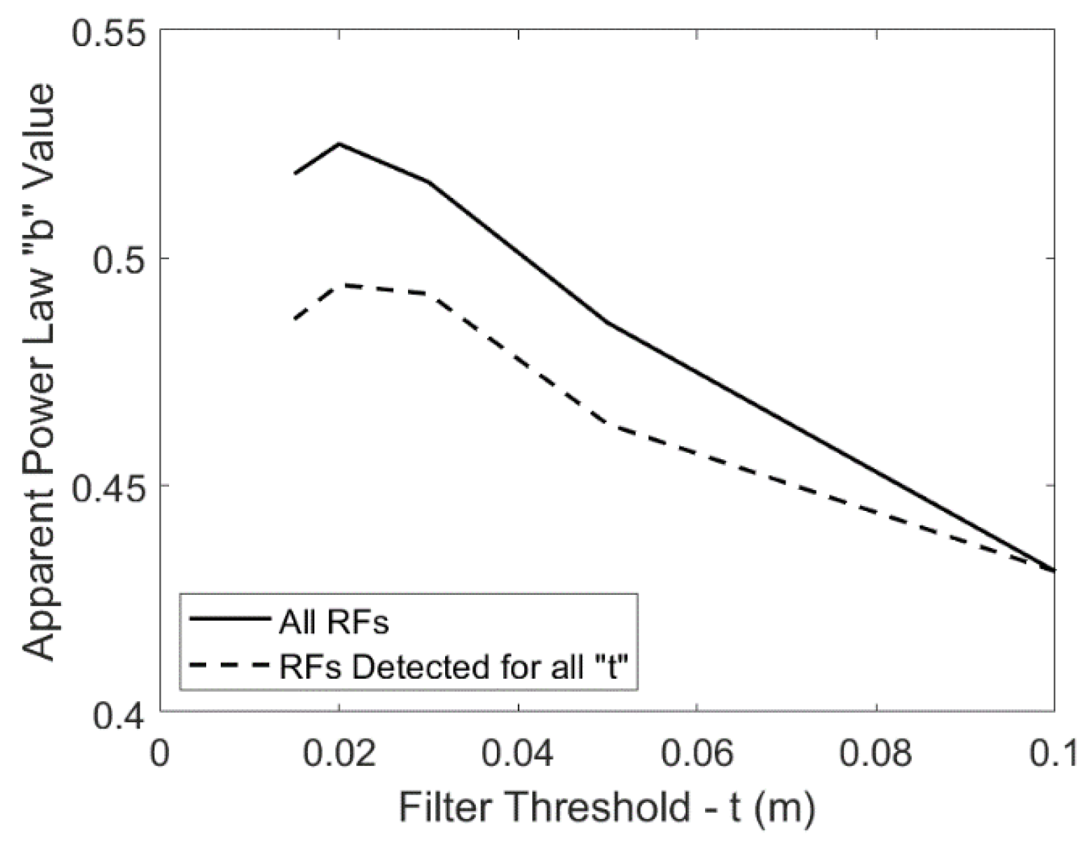
As in the case of the downsampling analysis, the disproportionate impact of change filter threshold on estimated volume for smaller rockfalls implies an impact on the slope of the resultant MCF curve. This impact is illustrated in Figure 16 for both all rockfalls detected for each t (Figure 16a) and only the subset of rockfalls that were identified in all cases tested (Figure 16b). The former MCF curves include both the influences of rockfall detectability (i.e., smaller rockfalls potentially not being identified for larger values of t), while the latter removes this effect and considers only the influence of processing parameters (t and Eps) on the volume (i.e., the effect illustrated in Figure 7a). For each of these cases, Figure 17 shows how the power law “b” parameter values (see Equation (1)) corresponding to the fits in Figure 16 vary depending on the value of t used.

4. Discussion

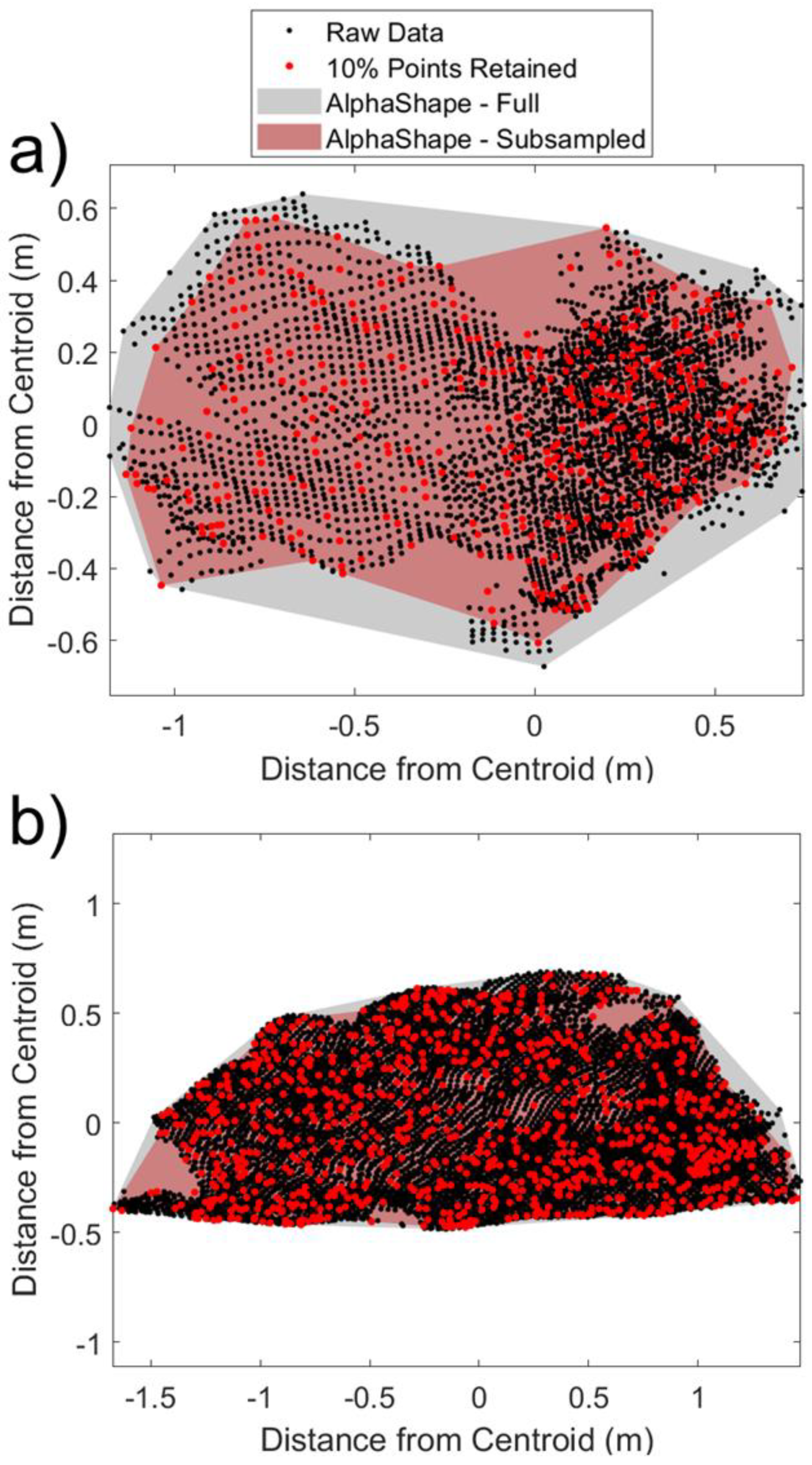
A limitation of this study is that the reference database used for all analyses only considered small rockfalls (< 10 m3), so the applicability to larger rockfalls is uncertain. However, we believe it can be inferred that for any given set of data quality conditions (point density and filter threshold), the degree of volume underestimation will decrease and become negligible as volume continues to increase. This represents an extrapolation of the empirical trends shown in Figure 9a,b and Figure 15a to larger volumes. This concept is illustrated in Figure 18 using a two-dimensional representation of two rockfalls of different sizes, for ease of visualization. The degree of volume underestimation can be considered as an “annulus” around the rockfall perimeter, and the thickness of the annulus is a function of data quality. For the smallest volumes at a given data quality, the annulus thickness is large relative to the rockfall diameter, but for larger volumes, variations constrained to an annulus of similar thickness have a negligible impact on volume estimation. Therefore, it is reasonable to expect that for even larger volumes than those considered in this study, the average impacts of data quality on rockfall volume estimates obtained using alphaSolid would be even less significant than for the largest volumes considered in this study (holding point density and other data factors constant).
Conversely, rockfalls that are small relative to any given data quality conditions are the most likely to have underestimated volumes. With respect to point spacing specifically, Figure 9e,f illustrate that as point spacing increases (lower point density), increasingly large rockfalls have their volumes underestimated by a notable amount (on average); we interpret this result to suggest that this effect of volume underestimation for smaller rockfalls will be present in larger-scale (e.g., regional) studies, in that regardless of the specific sizes of rockfalls identified, the smallest rockfalls that are identifiable using standard data-processing approaches will tend to be defined by relatively small numbers of points. This can be related to Figure 18 by the fact that the specific scale of the axes does not influence the overall trend. For a hypothetical regional monitoring campaign, a “small” rockfall, defined by a relatively small number of points, may be 10 m3 in volume, while a “large” rockfall may be 104 m3. In any case, we would expect smaller rockfalls to have a greater degree of underestimation.
Because of the disproportionate impacts on volume estimates for smaller rockfalls, the resolution and uncertainty effects tend to bias MCF curve results towards shallower slopes. This suggests that practical point spacing limitations and rockfall identification workflows tend to result in a relative underestimation of the proportion of small rockfalls as compared to large rockfalls. From a practical perspective, if one attempts to extrapolate such a trend for hazard assessment purposes, the relative frequency of especially large rockfalls will tend to be overestimated. The underestimation of the power law slope, b, due to resolution and uncertainty effects joins a series of other factors known to result in underestimation of b. It is notable, however, that the magnitude of the effect on b demonstrated in this study (approximately 0.05–0.08) is larger than that demonstrated for volume reconstruction method [22] and projection diameter used in the M3C2 change calculation [25], and is comparable to or greater than demonstrated temporal resolution effects [11,24], with the exception of the findings of Williams et al. [23].
Another relevant study is that of Benjamin et al. [34], who developed a rockfall database based on approximately four years of airborne lidar data for 24 km of coastline in the United Kingdom. They found that b was significantly underestimated (by as much as approximately 0.4) when evaluated using shorter segments of coastline, as compared to the value of b estimated using the full rockfall database. Accordingly, they suggested that power law parameters determined from monitoring of slopes with length less than 2.5 km could not be considered as representative of broader regional trends. Although they acknowledged the specific extent of monitoring necessary for a rockfall database to be considered representative (e.g., 2.5 km in the case of their study) would vary based on site-specific conditions (e.g., environmental conditions, lithological characteristics, etc.), the potential influence of data quality (and associated data-processing decisions) on this value was not explicitly addressed. Based on the findings of this study, we suggest that a portion of the decrease in b observed by Benjamin et al. [34] for smaller monitoring windows can likely be attributed to data quality effects. Specifically, for smaller monitoring windows, the decreased prevalence of events that are large relative to the average point spacing and value of t means that the values of b obtained are highly sensitive to the volume underestimation that occurs for the smallest (and more common) rockfall. We note that the data used by Benjamin et al. [34] had point spacings greater than 0.1 m, and a value of t = 0.1 m was used during data-processing, meaning it is likely that substantial underestimation of rockfall volumes occurred above the 0.001 m3 cutoff that they used for power law fitting. In other words, we hypothesize that if a higher resolution data set had been used along with a smaller value of t (and appropriate subsequent cluster filtering), the monitoring extent threshold above which the power law parameters become scale-invariant would have been lower than 2.5 km.
Although this study only demonstrates the effects of data quality on b for limited number of rockfalls with relatively small volumes at a single site, indirect evidence of the broader applicability of these effects exists within the literature. Specifically, Graber [38] performed a meta-analysis of published rockfall data to evaluate controls on the power law slope, b, including consideration of 27 studies that presented MCF curves developed based on terrestrial laser scanning data. Using these data, a linear regression showed a statistically significant (p < 0.05) relationship between the b value and the maximum volume present within a rockfall database. We interpret the maximum volume present within a rockfall database to be indirectly tied to the scale of the monitoring effort used to develop the database [34], and correspondingly, the resolution of the raw laser scanning data; although these relationships are not universal, it is common for larger monitoring areas to be sampled at a lower resolution due to increased scanner-to-target distance, likely also corresponding to higher change uncertainty and/or greater potential for alignment error [42,43]. Therefore, the resolution and uncertainty effects demonstrated in this paper provide a potential explanation for the relationship between maximum rockfall volume in a given database and the associated b value.
We note that this study is based on a data set collected using a specific laser scanner with specific settings, and it is assumed in our analysis that the reference database was produced using data with sufficiently high point density and precision to serve as a reliable point of comparison for the synthetic tests we conducted. The assumption of sufficient point density can be justified on the basis that the volume estimates obtained for removal of up to 50% of points returned similar volume estimates to the reference volume estimates on average (per Figure 9c), and by the restriction of the resolution analysis to volumes ≥ 0.1 m3. Regarding precision, it is true that the results for cases with noise added to individual points (Section 3.3) reflect results for point clouds with initial point error already present (i.e., due to imperfect reference database point cloud precision) in addition to the synthetically added noise. However, we estimate the two-standard-deviation precision for the reference database point clouds to be on the order of 2 cm or less (variable spatially and between different epochs); considering this in the context of the results for added noise presented in Figure 14, which shows notable average impacts of added noise on rockfall volume estimates only occur for two-stand-deviation added noise of ≥ 4 cm, suggests that the reference database point clouds have sufficient point precision to serve as a reliable basis for the analysis in the study.
We also note that the findings of this study should not be expected to necessarily apply to rockfall volume estimates derived using photogrammetric models. Specifically, when using lidar data, the raw input to the volume reconstruction algorithm is a set of points that are a relatively direct data representation of the rockfall geometry, where each point is independent from its neighbors; in contrast, the effective resolution and precision of photogrammetry models is influenced by several other parameters not mentioned here, including camera parameters, ground control quality, and lighting [44,45], all of which could influence volume estimation. Further research would be required to specifically evaluate these types of interactions.

5. Conclusions

This study evaluated the impacts of point cloud data quality attributes and associated filtering decisions on rockfall volume estimation. Specifically, using a reference database from a previous study, modifications to individual rockfall point cloud clusters were induced through downsampling, addition of gaussian noise to individual points, and reprocessing using a different change filter threshold value. Based on the tests conducted, it was determined that decreasing point spacing and increasing the change filter threshold both had the effect of, on average, decreasing the estimated rockfall volumes obtained for the smallest rockfalls considered. The disproportionate effect on volume estimation for small rockfalls were found to manifest as a decrease in the apparent power law slope, b, with a magnitude similar to or greater than what has previously been documented for most other data resolution or processing factors. Accordingly, this study has demonstrated an additional factor that tends to bias rockfall databases generated through repeated terrestrial laser scanning towards underestimation of the relative proportion of relatively small rockfalls. In future, this workflow could be applied using reference databases from different slopes to evaluate the extent to which slope-specific factors influence the magnitudes of the effects identified in this study.

Author Contributions

Conceptualization, G.W.; methodology, G.W. and L.W.; formal analysis, G.W. and L.W.; resources, G.W.; data curation, L.W.; writing—original draft preparation, G.W.; writing—review and editing, L.W.; project administration, G.W.; funding acquisition, G.W. All authors have read and agreed to the published version of the manuscript.

Funding

This research was funded by the Colorado Department of Transportation under Interagency Agreement 20-HAA-ZH-03024.

Data Availability Statement

Data are available upon request (contact G. Walton at [email protected]).

Acknowledgments

Efforts of Adam Malsam and other student members of the Computational Geomechanics Laboratory at the Colorado School of Mines to collect data at the Floyd Hill slope over the years are appreciated.

Conflicts of Interest

The authors declare no conflict of interest.

References

  1. Guerin, A.; Stock, G.M.; Radue, M.J.; Jaboyedoff, M.; Collins, B.D.; Matasci, B.; Avdievitch, N.; Derron, M.-H. Quantifying 40 years of rockfall activity in Yosemite Valley with historical Structure-from-Motion photogrammetry and terrestrial laser scanning. Geomorphology 2020, 356, 107069. [Google Scholar] [CrossRef]
  2. Rose, N.; Hungr, O. Forecasting potential rock slope failure in open pit mines using the inverse-velocity method. Int. J. Rock Mech. Min. Sci. 2006, 44, 308–320. [Google Scholar] [CrossRef]
  3. Budetta, P.; Nappi, M. Comparison between qualitative rockfall risk rating systems for a road affected by high traffic intensity. Nat. Hazards Earth Syst. Sci. 2013, 13, 1643–1653. [Google Scholar] [CrossRef] [Green Version]
  4. Lato, M.J.; Diederichs, M.S.; Hutchinson, D.J.; Harrap, R. Evaluating roadside rockmasses for rockfall hazards using LiDAR data: Optimizing data collection and processing protocols. Nat. Hazards 2011, 60, 831–864. [Google Scholar] [CrossRef]
  5. Corominas, J.; Mavrouli, O.; Ruiz-Carulla, R. Magnitude and frequency relations: Are there geological constraints to the rockfall size? Landslides 2017, 15, 829–845. [Google Scholar] [CrossRef] [Green Version]
  6. Kromer, R.; Lato, M.; Hutchinson, D.J.; Gauthier, D.; Edwards, T. Managing rockfall risk through baseline monitoring of precursors using a terrestrial laser scanner. Can. Geotech. J. 2017, 54, 953–967. [Google Scholar] [CrossRef]
  7. Bonneau, D.A.; Hutchinson, D.J. The use of terrestrial laser scanning for the characterization of a cliff-talus system in the Thompson River Valley, British Columbia, Canada. Geomorphology 2018, 327, 598–609. [Google Scholar] [CrossRef]
  8. Abellan, A.; Jaboyedoff, M.; Oppikofer, T.; Vilaplana, J.M. Detection of millimetric deformation using a terrestrial laser scanner: Experiment and application to a rockfall event. Nat. Hazards Earth Syst. Sci. 2009, 9, 365–372. [Google Scholar] [CrossRef] [Green Version]
  9. D’Amato, J.; Hantz, D.; Guerin, A.; Jaboyedoff, M.; Baillet, L.; Mariscal, A. Influence of meteorological factors on rockfall occurrence in a middle mountain limestone cliff. Nat. Hazards Earth Syst. Sci. 2016, 16, 719–735. [Google Scholar] [CrossRef] [Green Version]
  10. Jaboyedoff, M.; Oppikofer, T.; Abellán, A.; Derron, M.-H.; Loye, A.; Metzger, R.; Pedrazzini, A. Use of LIDAR in landslide investigations: A review. Nat. Hazards 2012, 61, 5–28. [Google Scholar] [CrossRef]
  11. Van Veen, M.; Hutchinson, D.J.; Kromer, R.; Lato, M.; Edwards, T. Effects of sampling interval on the frequency—Magnitude relationship of rockfalls detected from terrestrial laser scanning using semi-automated methods. Landslides 2017, 14, 1579–1592. [Google Scholar] [CrossRef]
  12. Williams, J.G.; Rosser, N.J.; Hardy, R.J.; Brain, M.J.; Afana, A.A. Optimising 4-D surface change detection: An approach for capturing rockfall magnitude–frequency. Earth Surf. Dyn. 2018, 6, 101–119. [Google Scholar] [CrossRef] [Green Version]
  13. Graber, A.; Santi, P. UAV-photogrammetry rockfall monitoring of natural slopes in Glenwood Canyon, CO, USA: Background activity and post-wildfire impacts. Landslides 2022, 1–20. [Google Scholar] [CrossRef]
  14. Kromer, R.; Walton, G.; Gray, B.; Lato, M.; Group, R. Development and Optimization of an Automated Fixed-Location Time Lapse Photogrammetric Rock Slope Monitoring System. Remote Sens. 2019, 11, 1890. [Google Scholar] [CrossRef] [Green Version]
  15. Blanch, X.; Abellan, A.; Guinau, M. Point Cloud Stacking: A Workflow to Enhance 3D Monitoring Capabilities Using Time-Lapse Cameras. Remote Sens. 2020, 12, 1240. [Google Scholar] [CrossRef]
  16. Tang, Y.; Huang, Z.; Chen, Z.; Chen, M.; Zhou, H.; Zhang, H.; Sun, J. Novel visual crack width measurement based on backbone double-scale features for improved detection automation. Eng. Struct. 2023, 274, 115158. [Google Scholar] [CrossRef]
  17. Farmakis, I.; Bonneau, D.; Hutchinson, D.J.; Vlachopoulos, N. Supervoxel-based multi-scale point cloud segmentation using fnea for object-oriented rock slope classification using tls. ISPRS-Int. Arch. Photogramm. Remote Sens. Spat. Inf. Sci. 2020, XLIII-B2-2, 1049–1056. [Google Scholar] [CrossRef]
  18. Farmakis, I.; Bonneau, D.; Hutchinson, D.; Vlachopoulos, N. Targeted Rock Slope Assessment Using Voxels and Object-Oriented Classification. Remote Sens. 2021, 13, 1354. [Google Scholar] [CrossRef]
  19. Farmakis, I.; DiFrancesco, P.-M.; Hutchinson, D.J.; Vlachopoulos, N. Rockfall detection using LiDAR and deep learning. Eng. Geol. 2022, 309, 106836. [Google Scholar] [CrossRef]
  20. Weidner, L.; Walton, G.; Kromer, R. Classification methods for point clouds in rock slope monitoring: A novel machine learning approach and comparative analysis. Eng. Geol. 2019, 263, 105326. [Google Scholar] [CrossRef]
  21. Abellán, A.; Oppikofer, T.; Jaboyedoff, M.; Rosser, N.J.; Lim, M.; Lato, M.J. Terrestrial laser scanning of rock slope instabilities. Earth Surf. Process. Landf. 2013, 39, 80–97. [Google Scholar] [CrossRef]
  22. DiFrancesco, P.-M.; Bonneau, D.; Hutchinson, D. Computational Geometry-Based Surface Reconstruction for Volume Estimation: A Case Study on Magnitude-Frequency Relations for a LiDAR-Derived Rockfall Inventory. ISPRS Int. J. Geo-Inf. 2021, 10, 157. [Google Scholar] [CrossRef]
  23. Williams, J.G.; Rosser, N.J.; Hardy, R.J.; Brain, M.J. The Importance of Monitoring Interval for Rockfall Magnitude-Frequency Estimation. J. Geophys. Res. Earth Surf. 2019, 124, 2841–2853. [Google Scholar] [CrossRef] [Green Version]
  24. Malsam, A.C.; Walton, G.; Schovanec, H.E.; Bonneau, D.A.; DiFrancesco, P.; Hutchinson, D.J. An Analysis of Seasonal Rockfall Trends at Floyd Hill: A Slope Along I-70, East of Idaho Springs, CO. In Proceedings of the 55th U.S. Rock Mechanics/Geomechanics Symposium, Online, 18–25 June 2021; Available online: https://onepetro.org/ARMAUSRMS/proceedings/ARMA21/All-ARMA21/ARMA-2021-1254/467974 (accessed on 6 October 2022).
  25. DiFrancesco, P.-M.; Bonneau, D.; Hutchinson, D.J. The Implications of M3C2 Projection Diameter on 3D Semi-Automated Rockfall Extraction from Sequential Terrestrial Laser Scanning Point Clouds. Remote Sens. 2020, 12, 1885. [Google Scholar] [CrossRef]
  26. Winiwarter, L.; Anders, K.; Höfle, B. M3C2-EP: Pushing the limits of 3D topographic point cloud change detection by error propagation. ISPRS J. Photogramm. Remote Sens. 2021, 178, 240–258. [Google Scholar] [CrossRef]
  27. Carrea, D.; Abellan, A.; Derron, M.-H.; Gauvin, N.; Jaboyedoff, M. MATLAB Virtual Toolbox for Retrospective Rockfall Source Detection and Volume Estimation Using 3D Point Clouds: A Case Study of a Subalpine Molasse Cliff. Geosciences 2021, 11, 75. [Google Scholar] [CrossRef]
  28. Bonneau, D.; DiFrancesco, P.-M.; Hutchinson, D.J. Surface Reconstruction for Three-Dimensional Rockfall Volumetric Analysis. ISPRS Int. J. Geo-Inf. 2019, 8, 548. [Google Scholar] [CrossRef] [Green Version]
  29. Weidner, L.; Walton, G. Monitoring the Effects of Slope Hazard Mitigation and Weather on Rockfall along a Colorado Highway Using Terrestrial Laser Scanning. Remote Sens. 2021, 13, 4584. [Google Scholar] [CrossRef]
  30. Amenta, N.; Choi, S.; Kolluri, R.K. The power crust. In Proceedings of the Sixth ACM Symposium on Solid Modeling and Applications, New York, NY, USA, 1 May 2001; pp. 249–266. [Google Scholar] [CrossRef]
  31. Malsam, A. Characterization of Rockfall Activity and Identification of Weather-Rockfall Relationships Using High Temporal Resolution Remote Sensing Methods. Master’s Thesis, Colorado School of Mines, Golden, CO, USA, 2022. [Google Scholar]
  32. Leonas, J. Mines Graduate Student and CDOT Work Together to Identify and Mitigate Rockslide on I-70–Before it Happened, Mines Newsroom. July 2022. Available online: https://www.minesnewsroom.com/news/mines-graduate-student-and-cdot-work-together-identify-and-mitigate-rockslide-i-70-it-happened (accessed on 12 December 2022).
  33. Westrum, M. I-70 WB Closed Nights at Floyd Hill, Rockfall Work, FOX31 Denver. March 2022. Available online: https://kdvr.com/news/local/i-70-wb-closed-nights-at-floyd-hill-rockfall-work/ (accessed on 12 December 2022).
  34. Benjamin, J.; Rosser, N.J.; Brain, M.J. Emergent characteristics of rockfall inventories captured at a regional scale. Earth Surf. Process. Landforms 2020, 45, 2773–2787. [Google Scholar] [CrossRef]
  35. Tonini, M.; Abellán, A. Rockfall detection from terrestrial LiDAR point clouds: A clustering approach using R. J. Spat. Inf. Sci. 2014, 8, 95–110. [Google Scholar] [CrossRef]
  36. Schovanec, H.; Walton, G.; Kromer, R.; Malsam, A. Development of Improved Semi-Automated Processing Algorithms for the Creation of Rockfall Databases. Remote Sens. 2021, 13, 1479. [Google Scholar] [CrossRef]
  37. Ester, M.; Kriegel, H.-P.; Sander, J.; Xu, X. A density-based algorithm for discovering clusters in large spatial databases with noise. In Proceedings of the Second International Conference on Knowledge Discovery and Data Mining (KDD-96), Portland, OR, USA, 2–4 August 1996; pp. 226–231. [Google Scholar]
  38. Graber, A. Understanding the Nuances of the Rockfall Frequency-Magnitude Relationship: Review and Examples from Two Original Case Studies in Glenwood Canyon, CO, USA. Ph.D. Thesis, Colorado School of Mines, Golden, CO, USA, 2022. [Google Scholar]
  39. Hungr, O.; Evans, S.G.; Hazzard, J. Magnitude and frequency of rock falls and rock slides along the main transportation corridors of southwestern British Columbia. Can. Geotech. J. 1999, 36, 224–238. [Google Scholar] [CrossRef]
  40. Clauset, A.; Shalizi, C.R.; Newman, M.E.J. Power-Law Distributions in Empirical Data. SIAM Rev. 2009, 51, 661–703. [Google Scholar] [CrossRef] [Green Version]
  41. Blanco, L.; García-Sellés, D.; Guinau, M.; Zoumpekas, T.; Puig, A.; Salamó, M.; Gratacós, O.; Muñoz, J.A.; Janeras, M.; Pedraza, O. Machine Learning-Based Rockfalls Detection with 3D Point Clouds, Example in the Montserrat Massif (Spain). Remote Sens. 2022, 14, 4306. [Google Scholar] [CrossRef]
  42. Kromer, R.A.; Hutchinson, D.J.; Lato, M.J.; Gauthier, D.; Edwards, T. Identifying rock slope failure precursors using LiDAR for transportation corridor hazard management. Eng. Geol. 2015, 195, 93–103. [Google Scholar] [CrossRef]
  43. Weidner, L.; Walton, G. Monitoring and Modeling of the DeBeque Canyon Landslide Complex in Three Dimensions. In Proceedings of the 54th U.S. Rock Mechanics/Geomechanics Symposium, Golden, CO, USA, 28 June–1 July 2020; Available online: https://onepetro.org/ARMAUSRMS/proceedings-abstract/ARMA20/All-ARMA20/ARMA-2020-1077/447457 (accessed on 5 October 2020).
  44. Karantanellis, E.; Arav, R.; Dille, A.; Lippl, S.; Marsy, G.; Torresani, L.; Elberink, S.O. Evaluating The Quality Of Photogrammetric Point-Clouds In Challenging Geo-Environments—A Case Study in An Alpine Valley. ISPRS—Int. Arch. Photogramm. Remote Sens. Spat. Inf. Sci. 2020, XLIII-B2-2, 1099–1105. [Google Scholar] [CrossRef]
  45. Westoby, M.J.; Lim, M.; Hogg, M.; Pound, M.J.; Dunlop, L.; Woodward, J. Cost-effective erosion monitoring of coastal cliffs. Coast. Eng. 2018, 138, 152–164. [Google Scholar] [CrossRef]
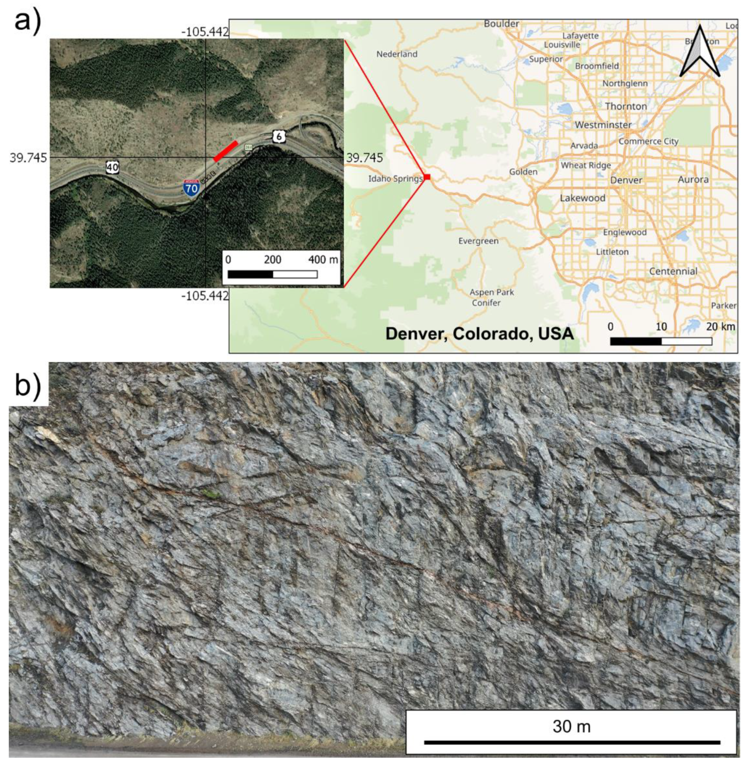
Figure 1. (a) Map of the monitoring location and (b) photography of the Floyd Hill slope rockmass. The red line on the inset map in (a) indicates the approximate location of the photograph shown in (b).
Remotesensing 15 00165 g001
Figure 2. Rockfall magnitude–cumulative–frequency curve for the Floyd Hill slope reference database with power law fit to volumes above 0.001 m3 shown [23].
Remotesensing 15 00165 g002
Figure 3. Two views of different parts of the Floyd Hill rock slope showing point clusters colored by date representing rockfalls exhibiting an elongated shape and sequential failure of adjacent blocks. (a) shows multiple smaller rockfall examples, and (b) shows 2017 rockfalls preceding a larger 2019 rockfall.
Remotesensing 15 00165 g003
Figure 4. Flowchart summarizing study methods.
Remotesensing 15 00165 g004
Figure 5. Example rockfall showing (a) the original point cloud, (b) the same point cloud randomly downsampled to 5% of the points, and (c,d) their respective alphaSolid reconstructed volumes (V = 0.46 m3 and V = 0.33 m3, respectively).
Remotesensing 15 00165 g005
Figure 6. Example rockfall showing (a) the original point cloud, (b) the same point cloud with 0.005 m of gaussian random noise added in all three co-ordinate directions, and (c,d) their respective alphaSolid reconstructed volumes (V = 0.46 m3 and V = 0.31 m3, respectively).
Remotesensing 15 00165 g006
Figure 7. Example rockfall cluster showing (a) a front view of clustered points for the t = 0.015 m (red) and t = 0.100 m cases (black), (b) views of the reconstructed alphaSolid mesh for the t = 0.015 m cluster (V = 3.15 m3), and (c) views of the reconstructed alphaSolid mesh for the t = 0.100 m (V = 2.41 m3) cluster.
Remotesensing 15 00165 g007
Figure 8. Example log-linear trend in estimated rockfall volumes as a function of t. A “Log-Slope” of −0.024 per cm Δt indicates that for each cm of increase in t, for this particular rockfall, the base 10 logarithm of the estimated volume decreases by 0.024.
Remotesensing 15 00165 g008
Figure 9. Downsampling test results for (a,c,e) random downsampling and (b,d,f) voxel downsampling. The “x”s in (e,f) represent the center points of each reference volume “bin” used to determine the average downsampled volume estimates that have been contoured.
Remotesensing 15 00165 g009
Figure 10. Downsampling test results for (a) random and (b) voxel downsampling, with results for individual rockfalls connected by lines, and the mean result at each downsampling level shown in red.
Remotesensing 15 00165 g010
Figure 11. (a) Minimum and (b) maximum volume estimates across 200 random downsampling cases for each reference rockfall.
Remotesensing 15 00165 g011
Figure 12. Magnitude–cumulative–frequency (MCF) curves for different levels of (a) random and (b) voxel downsampling; note that lvoxel represents the edge length of the voxels used for downsampling.
Remotesensing 15 00165 g012
Figure 13. Power law “b” values for different degrees of (a) random and (b) voxel downsampling.
Remotesensing 15 00165 g013
Figure 14. Point precision test results, with results for individual rockfalls connected by lines, and the mean result for each level of added noise shown in red.
Remotesensing 15 00165 g014
Figure 15. Results from linear regressions of estimated volume versus change filter threshold showing (a) log-slope values as a function of reference volume and (b) degree of log-linear data-model fit, as quantified by R2; (c) representative examples of how the slope trend displayed in (a) manifests in terms of the influence of t on volume estimates for rockfalls of different sizes.
Remotesensing 15 00165 g015
Figure 16. Magnitude–cumulative–frequency (MCF) curves obtained using various filter thresholds considering (a) all detected rockfall clusters for each given threshold and (b) only rockfall clusters that were identified for all threshold cases.
Remotesensing 15 00165 g016
Figure 17. Power law “b” values for different change filter threshold (t) cases.
Remotesensing 15 00165 g017
Figure 18. Two-dimensional representations of points corresponding to a (a) smaller (0.46 m3) and (b) larger (1.21 m2) rockfalls, with and without subsampling, and their corresponding alphaSolid representations. In both cases, the changes in the alphaSolid representation associated with subsampling are constrained to an “annulus” with a thickness on the order of approximately 0.1 m.
Remotesensing 15 00165 g018
Table 1. Filter threshold (t) and search radius (Eps) parameter combinations.
t (m)Eps (m)
0.0150.07
0.0200.10
0.0300.12
0.0500.15
0.1000.20
Table 2. Number of candidate clusters and final post-filtering rockfall matches for each change filter threshold case.
t (m)# of Candidate Clusters# of Rockfall Matches
0.015193155
0.020193173
0.030184168
0.05011875
0.1003728
Disclaimer/Publisher’s Note: The statements, opinions and data contained in all publications are solely those of the individual author(s) and contributor(s) and not of MDPI and/or the editor(s). MDPI and/or the editor(s) disclaim responsibility for any injury to people or property resulting from any ideas, methods, instructions or products referred to in the content.