Article

Multi-Domain Fusion Graph Network for Semi-Supervised PolSAR Image Classification

School of Electronic Information, Wuhan University, Wuhan 430079, China
*
Author to whom correspondence should be addressed.
Remote Sens. 2023, 15(1), 160; https://doi.org/10.3390/rs15010160
Submission received: 19 October 2022 / Revised: 21 December 2022 / Accepted: 25 December 2022 / Published: 27 December 2022
(This article belongs to the Section Remote Sensing Image Processing)

Abstract

:
The expensive acquisition of labeled data limits the practical use of supervised learning on polarimetric synthetic aperture radar (PolSAR) image analysis. Semi-supervised learning has attracted considerable attention as it can utilize few labeled data and very many unlabeled data. The scattering response of PolSAR data is strongly spatial distribution dependent, which provides rich information about land-cover properties. In this paper, we propose a semi-supervised learning method named multi-domain fusion graph network (MDFGN) to explore the multi-domain fused features including spatial domain and feature domain. Three major factors strengthen the proposed method for PolSAR image analysis. Firstly, we propose a novel sample selection criterion to select reliable unlabeled data for training set expansion. Multi-domain fusion graph is proposed to improve the feature diversity by extending the sample selection from the feature domain to the spatial-feature fusion domain. In this way, the selecting accuracy is improved. By few labeled data, very many accurate unlabeled data are obtained. Secondly, multi-model triplet encoder is proposed to achieve superior feature extraction. Equipped with triplet loss, limited training samples are fully utilized. For expanding training samples with different patch sizes, multiple models are obtained for the fused classification result acquisition. Thirdly, multi-level fusion strategy is proposed to apply different image patch sizes for different expanded training data and obtain the fused classification result. The experiments are conducted on Radarsat-2 and AIRSAR images. With few labeled samples (about 0.003–0.007%), the overall accuracy of the proposed method ranges between 94.78% and 99.24%, which demonstrates the proposed method’s robustness and excellence.

1. Introduction

In recent years, we have seen a remarkable growth of using deep learning to help understand remote sensing images [1,2,3]. Following this trend, deep neural networks have demonstrated empirical success in SAR data interpretation [4,5,6]. These deep neural networks are trained via a supervised learning paradigm: given massive labeled SAR data [7,8,9,10,11,12,13,14,15,16]. However, the acquisition of labeled SAR data is expensive: only experts with specific geoscience knowledge are invited to identify the propriety of an area from their experience. Moreover, this requirement for human labor limits the speed of data labeling. As a result, we are left with small amounts of labeled SAR data but large amounts of unlabeled SAR data.
The rise of semi-supervised learning provides a solution to perform better PolSAR data interpretation with limited labeled data and the help from massive unlabeled data [17,18,19,20,21,22]. Semi-supervised learning (SSL) [23,24] refers to algorithms that improve the learning by generating pseudo-labels for unlabeled data using knowledge from labeled data.
In our work, we provide a novel SSL solution for PolSAR data interpretation. We propose a multi-domain fusion graph network (MDFGN) to model multi-domain fused features. Compared to the previous SSL works, MDFGN has the following features:
A Novel Sample Selection Criterion: We design a sample selection criterion based on multi-domain fusion graph (MDFG) to select unlabeled data in the spatial-feature fusion domain. In current SSL methods, unlabeled samples are selected relying on the extracted features, that is, only in the feature domain. The diversity of selecting domains can enhance the reliability of the selected samples. The spatial distribution homogeneity of PolSAR images contains rich information beyond polarimetric features: spatially adjacent pixels in PolSAR image have more similar semantics than pixels that are far apart geographically [25]. To make use of the rich information in the spatial domain, we define multi-domain fusion confidence (MDFC) as the classification confidence in the spatial-feature fusion domain. The labeled samples have the highest MDFC as 1 and the unlabeled samples with a high MDFC are considered reliable. To search the reliable samples from large amounts of unlabeled PolSAR data, nearest neighbor graph (NNG) structure [26] is applied for low search complexity. MDFG is an NNG with vertices corresponding to the labeled and unlabeled data, edges corresponding to MDFC to links between vertices and a searching algorithm.
An Effective Feature Extractor: We design a multi-model triplet encoder for feature extraction. Our encoder is similar to metric learning [27,28]. Our proposed encoder is trained on PolSAR data triplets, where each triplet consists of three image patches sampled randomly from a training set. In the triplet, two PolSAR patches are in the same category and the others in different categories. The proposed encoder favors a small euclidean distance between pairs of the feature vectors of image patches in the same category and a large distance between the feature vectors in different categories. Training triplets are sampled and combined randomly from labeled samples and the training set is expanded, which alleviates the overfitting caused by insufficient labeled data. Explicit representation provides a metric method for the feature domain to select samples in the feature domain. To classify a pixel of PolSAR images, the image patch whose center is the pixel is obtained and the feature is extracted by the convolutional layer. The classification process takes the extracted features as the input and outputs the land-cover category corresponding to the central pixel of the input patch. Classification is carried out at the patch level, so different image patch sizes definitely lead to different classification results [29,30]. Due to the effect of PolSAR image speckle noise, the big image patch leads to low accuracy at the small, narrow or junction areas, but less noise in the classification results. While the small patch leads to more noise, the detail retention is better. Inspired by these foundations, patch size is selected flexibly according to the distribution of training data to adequately capture both microtextures and macrotextures in the original PolSAR image. After several sample selections, multi-models are obtained according to multi-training sets and patch sizes.
A Multi-level Fusion Strategy: A multi-level fusion strategy is proposed to obtain accurate classification result. Classical SSL obtains merely one model and classification result after selecting samples. In contrast, with several selecting loops, MDFGN applies appropriate patch size and retains every model for each selecting loop. The fused classification result is weighted and combined by the classification results with different training model and patch sizes to achieve a tradeoff between the noise control and detail retention.
The main contributions of this work are as follows.
(1)
A novel sample selection criterion based on multi-domain fusion graph to model multi-domain fused features, leading MDFGN to select unlabeled data accurately in the spatial-and-feature domain.
(2)
A multi-model triplet encoder is proposed to improve the discrimination and robustness of feature extraction from few labeled data. Image patch size is selected flexibly for different expanding training samples to capture both microtextures and macrotextures and multiple models are obtained for the fused classification result acquisition.
(3)
A multi-level fusion strategy is proposed to achieve the tradeoff with the noise control and detail retention.
The remainder of this article is organized as follows. In Section 2, NNG and triplet network are introduced. In Section 3, the proposed semi-supervised method is presented. Section 4 and Section 5 describe the datasets, the experimental settings and the results and discussion. Conclusions are drawn in Section 6.

2. Related Work

2.1. Nearest Neighbor Graph

Each PolSAR image has millions or even tens of millions of pixels. The application of nearest neighbor graph (NNG) can significantly speed up massive high-dimensional feature vector calculation and obtain low search complexity.
Nearest neighbor search based on graph structure has attracted attention in the fields of computer vision and multimedia search due to its excellent performance. In Refs. [31,32,33], some graph-based methods for hyperspectral image classification are proposed. One of the generally used approaches is K-nearest neighbor search (K-NNS), but it has poor performance on clustered data. In Refs. [34,35], authors proposed a proximity graph K-NNS algorithm called navigable small world (NSW). NSW utilizes navigable graphs, i.e., graphs with logarithmic or polylogarithmic scaling of the number of hops during the greedy traversal with respect to the network size [36,37]. NSW is constructed via consecutive insertion of elements in random order by bidirectionally connecting them to the M closest neighbors from the previously inserted elements. In Ref. [26], a new approach for the approximate K-NNS based on NSW with controllable hierarchy (Hierarchical NSW, HNSW) is proposed. HNSW is fully graph-based without any need for additional search structures, as shown in Figure 1. Closest neighbors at each layer are found by a variant of the greedy search algorithm. For every inserted element, an integer maximum layer is randomly selected with an exponentially decaying probability distribution. HNSW offers an excellent performance and is a clear leader on a large variety of the datasets, surpassing the opensource rivals by a large margin in cases of high-dimensional data. So HNSW is applied for the feature vector calculation and classification tasks in the proposed algorithm due to the excellent performance.

2.2. Triplet Network

The high dimensionality often introduces challenges for the conventional data analysis techniques. In order to improve the classification performance of PolSAR images, deep metric learning is often introduced to assign small distances between samples from the same class and large distances from different classes. More recently, deep learning methods have shown a great potential to uncover highly discriminating features in PolSAR images, with the so-called deep metric learning approach being one of the most prominent trends [38,39]. Deep metric learning aims at projecting semantically similar input data to nearby locations in the final feature space, which is highly appropriate to manage complex PolSAR data [40].
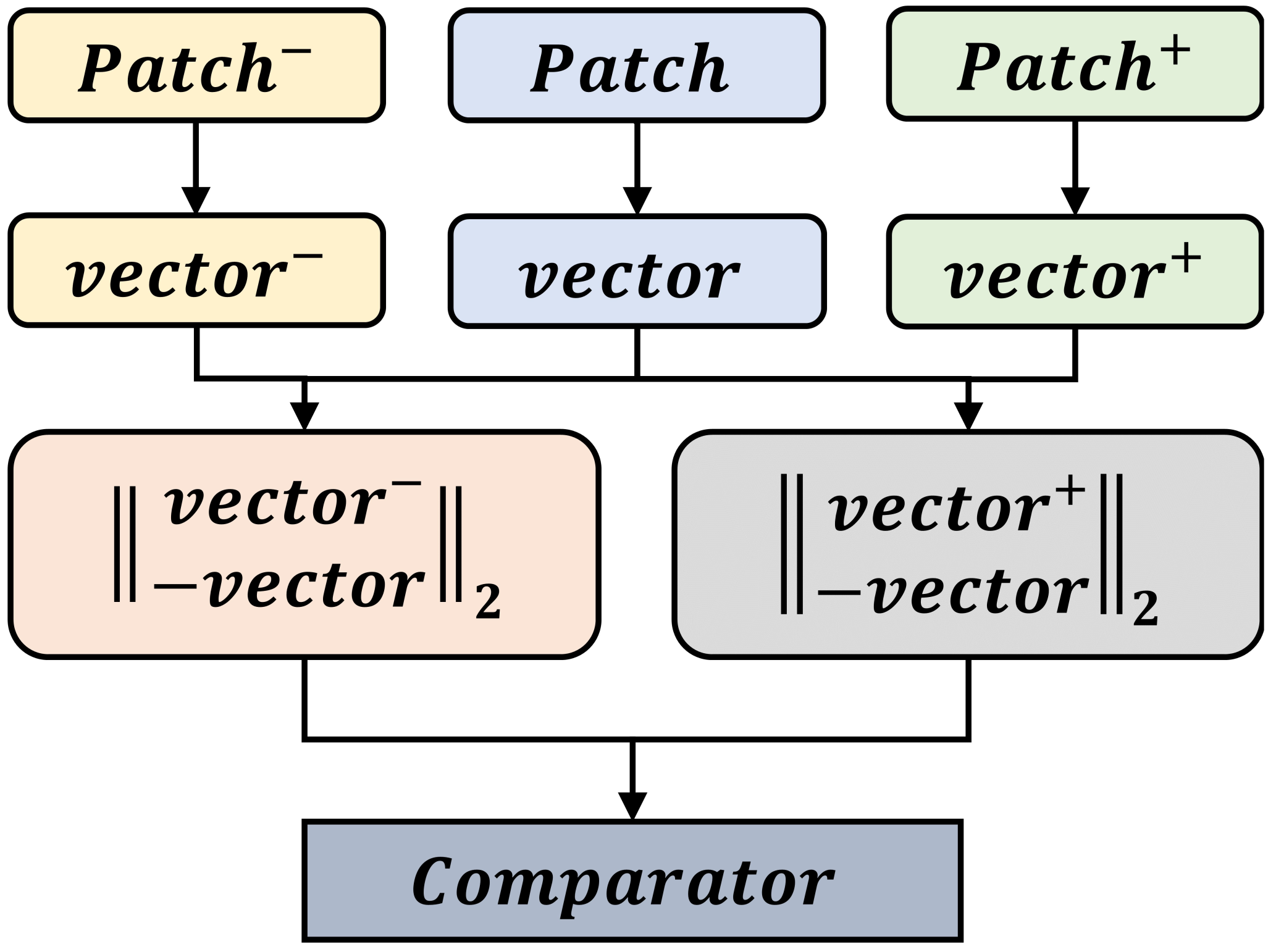
In Ref. [27], authors propose the triplet network based on metric learning, which aims to learn useful representations by distance comparisons. A triplet network is comprised of three instances of the same feed-forward network. When fed with three samples, the network outputs two intermediate values minus the L2 distances between the embedded representation of two of its inputs from the representation of the third. If we denote the three inputs as p a t c h , p a t c h + and p a t c h , and the embedded representation of the network as N e t ( p a t c h ) , the one before last layer will be vector:
v = N e t ( p a t c h ) N e t ( p a t c h ) 2 N e t ( p a t c h ) N e t ( p a t c h + ) 2 R
This network allows learning by comparisons of image patches instead of direct data labels. However, the efficient feature extraction network was not implemented in Figure 2. The application of the triplet network in PolSAR classification is limited due to the disappearance of the gradient. So we propose a multi-model triplet encoder, where each layer receives collective knowledge from the previous layers by cascading methods. Multi-model triplet encoder has better performance for classification tasks with strong interference and high noise, such as PolSAR image classification.

3. Materials and Methods

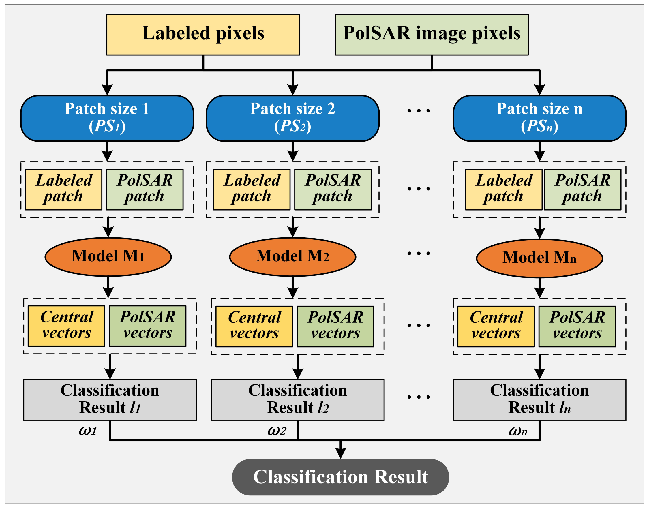
The architecture of the proposed MDFGN for PolSAR image classification is demonstrated in Figure 3. Taking the PolSAR coherency matrix as input, the well trained multi-model triplet encoder acquired in the training phase is used to obtain multiple classification results. With the multi-level fusion strategy, the classification result of each model combines with a certain weight to form the fused classification result. During the training phase, cooperating with the specialized training strategy, the MDFGN obtains a highly comprehensive representation of PolSAR data. Taking the PolSAR coherency matrix as input, the labeled pixels are selected randomly and unlabeled pixels are sampled evenly from the coherency matrix. The features of the coherency matrix are learned and trained by the multi-model triplet encoder. For the proposed sample selection criterion, a multi-domain fusion graph (MDFG) is built by the feature vectors of labeled patches ( v l ) and unlabeled patches ( v u ) and the spatial position of labeled samples ( p l ) and unlabeled samples ( p u ). Then, accurate unlabeled samples are selected. In the patch size module, adapted patch size is decided to obtain the selected image patches according to the distribution of selected samples. Selected patches are added into the training set and the multi-model triplet encoder will receive further positive training to obtain the new model. Detailed descriptions of the proposed architecture are as follows.

3.1. Sample Selection Criterion

For PolSAR images, spatially adjacent image patches should have similar semantics and share the same label, while patches far apart are likely to have different labels. Multi-domain fusion confidence (MDFC) is defined as the multi-domain fusion similarity distance between the unlabeled samples and the labeled samples. The MDFC of labeled data is highest as 1 because of the 100 % accuracy, while the classification confidence of unlabeled samples is considered from two domains:
(1)
Feature domain. Unlabeled samples with a small feature vector similarity distance with labeled samples have high classification confidence in the feature domain.
(2)
Spatial domain. For the homogeneity of spatial distribution of land-cover categories, unlabeled samples that are spatially close to labeled samples have high classification confidence in the spatial domain.
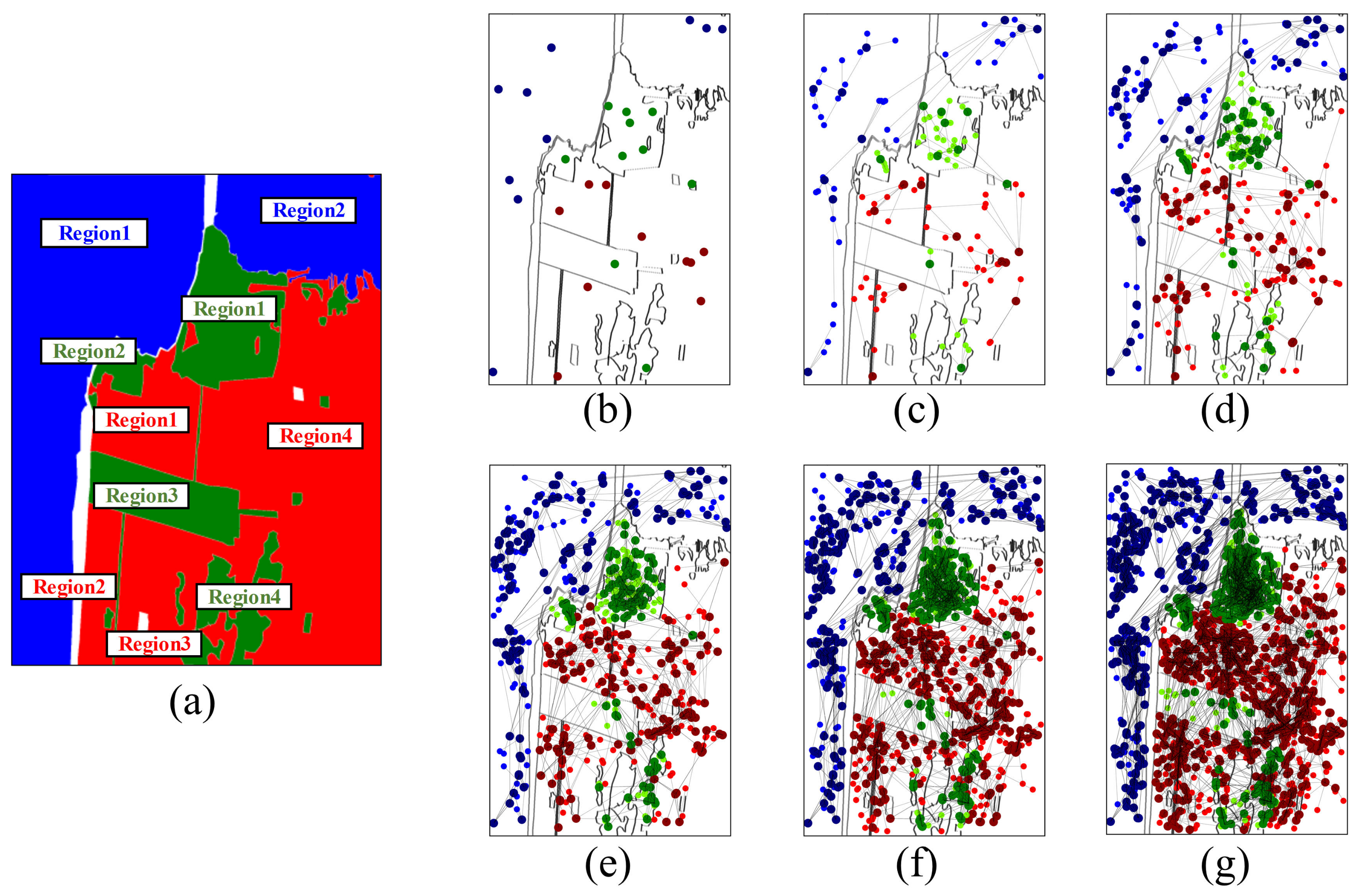
Algorithm 1 summarizes the MDFG calculation process. Firstly, labeled patches and unlabeled patches are extracted to feature vectors. Central vector of each category is obtained and classification is processed to generate a pseudo-label for unlabeled samples. In each category, the NNG of feature vectors (NNG f ) is built with vertices that are the feature vectors of unlabeled samples and edges that are the distances between vertices. The feature vectors of labeled samples are entry points to select candidate samples. The candidate samples have feature vectors similar to the labeled samples for further accurate selection. Then, the normalized spatial distance between the labeled samples and candidate samples are used as the weight of the edges to change the structure of NNG f . We call the new graph the multi-domain fusion graph (MDFG), where MDFCs are vertices and the fusion distances between vertices are edges. According to MDFG, unlabeled samples with big MDFCs are selected. The selected samples make full use of the deep feature and have high similarity with the labeled samples in the feature domain, and also make full use of the spatial homogeneity of the PolSAR image and are geographically close to the labeled samples. MDFC is normalized in the range [0, 1], shown in Figure 4. For each labeled sample, three unlabeled samples are selected and connected to the labeled samples, as shown in Figure 5c–g.
Algorithm 1 MDFG algorithm
 1:
Input:
  • Feature normalization factor: α , spatial normalization factor: β , the unlabeled image patches ( p t h u ) and their spatial position ( p u ), the labeled image patches ( p t h l ) and spatial position ( p l k , k = 1, 2, ⋯, K) of K categories, K is the category number, training model (Net)
 2:
Feature vectors are extracted by model:
  •     v u = Net( p t h u ).
  •     v l = Net( p t h l ).
 3:
Get central vector per category:
 4:
for each class k K  do
 5:
   Get the central vector: v c k = sum( v l k )/number( v l k )
 6:
end for
 7:
Classify the unlabled data:
  •     l v u ⇐ argmin( d ( v u , v c 1 ) , … , d ( v u , v c K ) )
 8:
for each class k K  do
 9:
   for each labeled data do
 10:
     Build NNG of extracted feature vectors and get 1000 nearest vectors as candidate samples.
 11:
     Compute the feature confidence ( d f ), position confidence ( d p ) and MDFC of candidate unlabeled samples ( v u , s u , l v u ):
  •       d f = v l v u v l k = l v u 2 k v u v c k l v u 2
  •       d p = p l p u p l k = l v u 2
  •       α = ln ( ϕ ) m a x ( d f ) , β = ln ( ϕ ) m a x ( d p ) , ϕ = 0.99
  •      MDFC = e α d f × e β d p
 12:
     MDFG is obtained by rebuilding the structure of NNG in feature domain.
 13:
     For each labeled sample, three samples with biggest MDFC are searched.
 14:
   end for
 15:
end for
 16:
Output: MDFG, selected samples.
PolSAR images have regional characteristics. Each region is separated by other land-cover categories, shown in Figure 5. The blue part (Water) in Figure 5a can be divided into two regions and the green (Forest) and red (Building) parts can be divided into four regions. In each selecting loop, most of the selected unlabeled samples are in the same region as the connected labeled samples due to the spatial restriction of MDFC. However, if the feature vectors of some unlabeled samples are sufficiently close to labeled samples, MDFC exhibits biases towards the feature domain to select the cross-regional samples. The first training set has only one or two samples or even no samples in each region, as shown in Figure 5b. After five selection loops, MDFC selects massive samples in all regions and connects them together. Figure 5b shows the first training set of labeled samples. Figure 5c–g show the expanded training set after one-five selection loops.
For MDFG, the dual restriction of feature domain and spatial domain improves the reliability of sample selection. Sample selection based on MDFG not only depends on the performance of feature extractor which is limited by noise interference and little supervised information. MDFG obtains the label of massive unlabeled samples accurately with few labeled samples and adds the selected unlabeled samples to the training set for further positive training.

3.2. Multi-Model Triplet Encoder

Multi-model triplet encoder is proposed at the level of image patches, as shown in Figure 6. It is composed of one convolution layer, three denseblock layers, two transition layers and one BN layer. Each layer receives collective knowledge from the previous layers by cascading methods which effectively solves the problem of gradient disappearance.
N c × N l image patches with centers that are labeled pixels are the input to the network ( N c is the number of land-cover categories; N l is the number of labeled samples for each category). Two land-cover categories are selected randomly and three image patches selected from the two categories constitute a triplet. To learn a mapping from image patches to low-dimensional embeddings, the encoder projects down the dimension and extracts the feature from the triplet. Each image patch is extracted to a 1 × 512 feature vector, so each triplet patch is transformed to a triplet of feature vectors ( v , v + , v ). v and v + are in the same category and v is in a different category. The encoder expresses the task as a multi-class classification problem, where the objective is to correctly classify which of v + and v have the same land-cover category as v . The label or pseudo-label determines which vector is closer to v .
The loss function is defined as triplet loss. Triplet loss favors minimizing Euclidean distance between pairs of feature vectors in the same category and maximizing Euclidean distance between pairs of vectors in different categories. Here “a small distance” is interpreted as “sharing the same label”. In order to output a comparison operator from the model, a softplus function is applied on outputs—effectively creating a ratio measure. Triplet loss is defined as follows:
l o s s = s o f t p l u s ( d + d + m a r g i n )
where m a r g i n is an offset.
d + = v v + 2 d = v v 2
Triplet loss is calculated by the distance of feature vectors not the predicted label. Classical SSL methods have overfitting problems due to there being little supervised information. In contrast, triplet encoder effectively reduces the risk of overfitting from two aspects. Firstly, the classical deep learning network uses the predicted label of training data as loss. If the training accuracy is high enough, the loss is difficult to drop. Overtraining will lead to overfitting. In contrast, triplet loss is the distance of the feature vectors. Even if the training accuracy is already very high, the triplet encoder can train further to make the intra-class distance smaller and the inter-class distance larger, which increases the robustness of the model and threshold for overtraining. Secondly, triplet loss expands the training set. Random sampling and combinating also resamples the training data to further utilize labeled samples. If there are N c land-cover categories and N l labeled samples per category. In the classical deep learning network, the size of the training set is: N c × N l . While the size of the training set of the triplet encoder is 2 N c × 2 N l × 1 N l , which effectively expands the training set.
We later observe that better feature extraction is achieved with the triplet loss and random sampling and combinating. To compare the classification accuracy and robustness of the multi-model triplet encoder and the classical deep learning network on PolSAR images, we design an experiment in Section 4.

3.3. Patch Size Module

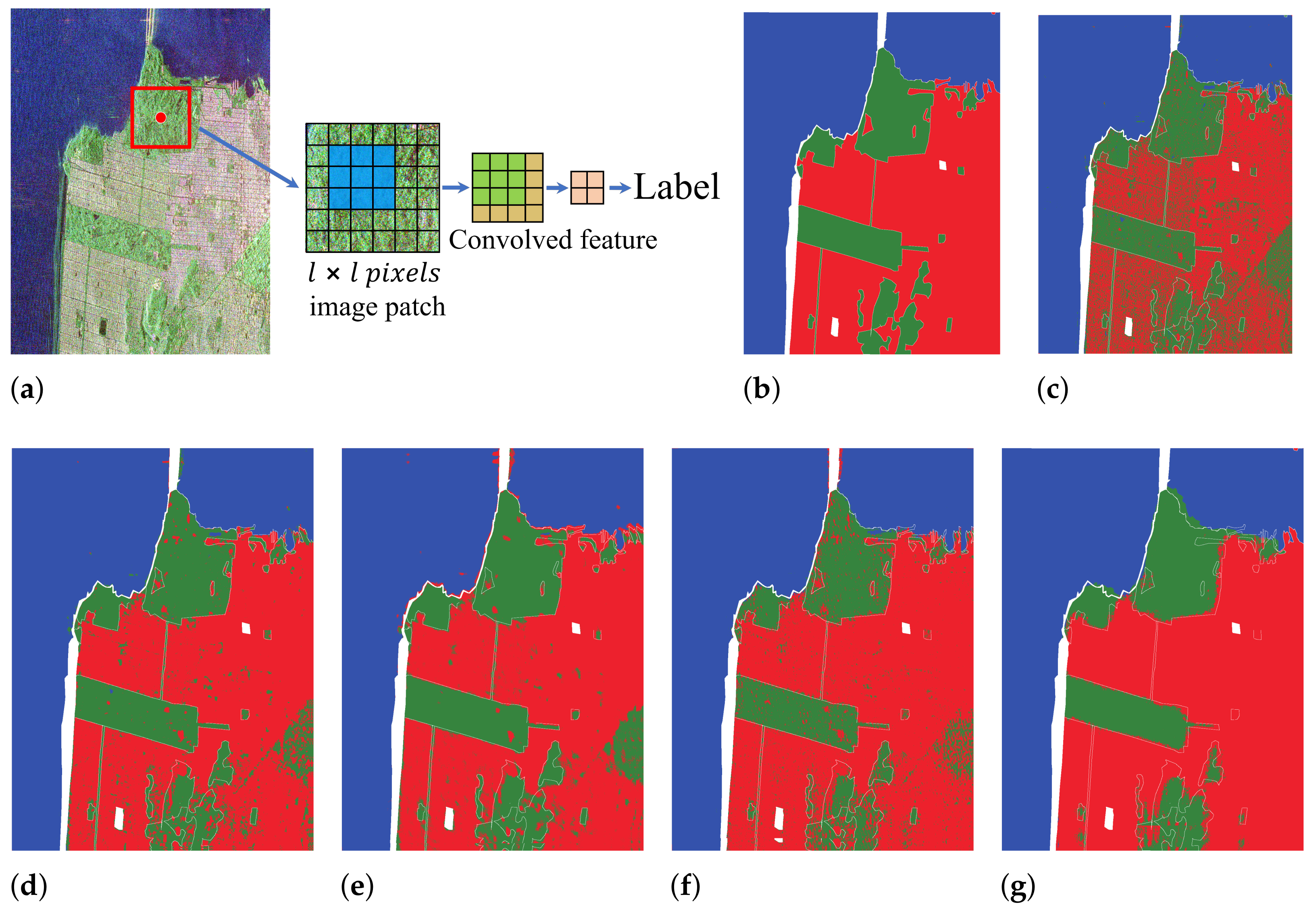
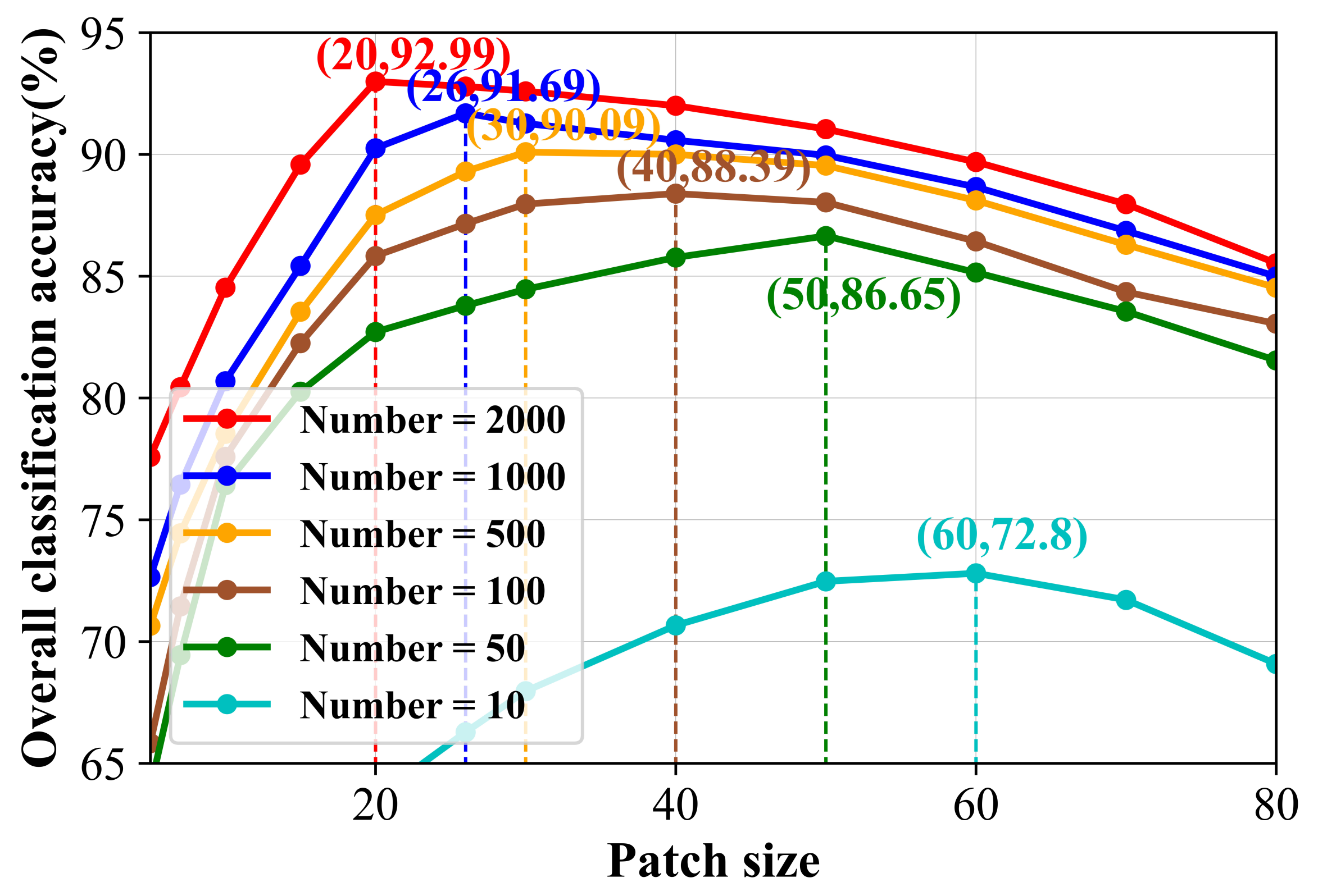
As the training set expands, image patch size is selected flexibly to obtain the best classification result. Due to coherent speckle noise, the feature of image patch is influenced by the noise pixels. Large patch size makes the image patch represent the pixel better, but results in low accuracy in the small, narrow or junction areas. While small patch size leads to noise points, but detail retention is better. Appropriate patch size can achieve the tradeoff between the noise control and detail retention. In the example of land-cover classification using ResNet on Rs2-Sanf data as shown in Figure 7, the results using small patch size have a lot of noise points, but the accuracy is high in the junction, small and narrow areas, and detail retention is better. While the results using big patch size have few noise points, the accuracy is low in the junction, small and narrow areas. With few labeled samples, microtexture is hard to capture. So large patch size is applied to capture macrotexture and the best result can be obtained. With a large amount of labeled samples, small patch size is applied to capture microtexture and the best result can be obtained. From the result shown in Figure 8, the patch size that achieves highest accuracy is larger when there are fewer labeled samples and the patch size with highest accuracy is smaller when the number of labeled samples is larger.
Since there are few labeled samples in the initial selection loop, the large patch is applied. As the sample selection progresses, the smaller patch size is appropriate. The image patch size is defined as follows:
p s k = k × i t v l p s i n i N t + p s i n i
where p s k is the patch size in the kth selecting loop, i t v l is the sampling interval when sampling the unlabeled samples evenly from the PolSAR image, p s i n i is the initial patch size and N t is the number of selection loops.

3.4. Multi-Level Fusion Strategy

The classification process is shown in Figure 9. The multi-leveled fusion strategy is proposed to obtain the accurate classification result and achieve the tradeoff between noise control and detail retention.
The patch size in the kth selecting loop is p s k . The model of the kth selection loop is m o d e l M k (k = 1, 2, ⋯, N t ). According to p s k , labeled patches centered on every labeled pixel and PolSAR patches centered on every pixel of PolSAR image are obtained. The central vector ( v c ) of each land-cover category is obtained by averaging the feature vectors ( v l ) transformed by the m o d e l M from labeled image patches having the same label. The PolSAR image patches of each pixel are transformed into a 1 × 342 feature vector ( v ) by the m o d e l M. Then, the label of the feature vector v ( l v ) can be obtained as follows:
v = M ( p a t c h )
v c n = ( v l n ) / n u m ( v l n ) ( 1 n N c )
l v = a r g m i n ( d ( v , v c 1 ) , d ( v , v c 2 ) , , d ( v , v c N c ) )
d ( v , v c n ) = v v c n 2
where v c n is the central vector of land-cover category n and N c is the number of land-cover categories.
With N t patch sizes and training models, N t classification results can be obtained. The classification results obtained by the model in the initial sample selection have less noise, but the classifications of junction areas and detail retention are poor. The classification results in the later sample selection achieve higher accuracy at the junction areas, but there is more noise. Since noise is random, we weight all classification results to achieve a tradeoff between detail preservation and noise control. In order to have less noise in the final classification results, the initial classification results have a large weight. The later classification results can be weighted and combined to eliminate noise and achieve high accuracy on junction, small or narrow areas. The label of final classification result ( l f ) is:
l f = k = 1 N t ω k l k
where l k is the label in the classification result by model M k and ω k is the weight of l k . A large patch size is applied to improve the accuracy of macrotextures and a small patch size is applied to capture the microtextures. To maintain macrotexture accuracy and control the noise, large weight is set to large patch and small weight is set to small patch. The distribution of noise is random, so a weighted combination can eliminate noise and maintain microtexture accuracy. To make each classification result play a role in the final result and the weight of each classification result suitable, the weight is set as follows: ω 1 > ω 2 > > ω N t and ω 1 < 2 × ω N t .

4. Results

In this section, the experimental data are first introduced. Then, the classification results are obtained by the proposed method and compared methods are presented and the performance of the proposed method with few labeled samples is discussed. The ablation study and detailed analysis of the proposed method are also discussed.

4.1. Dataset Descriptions and Experimental Settings

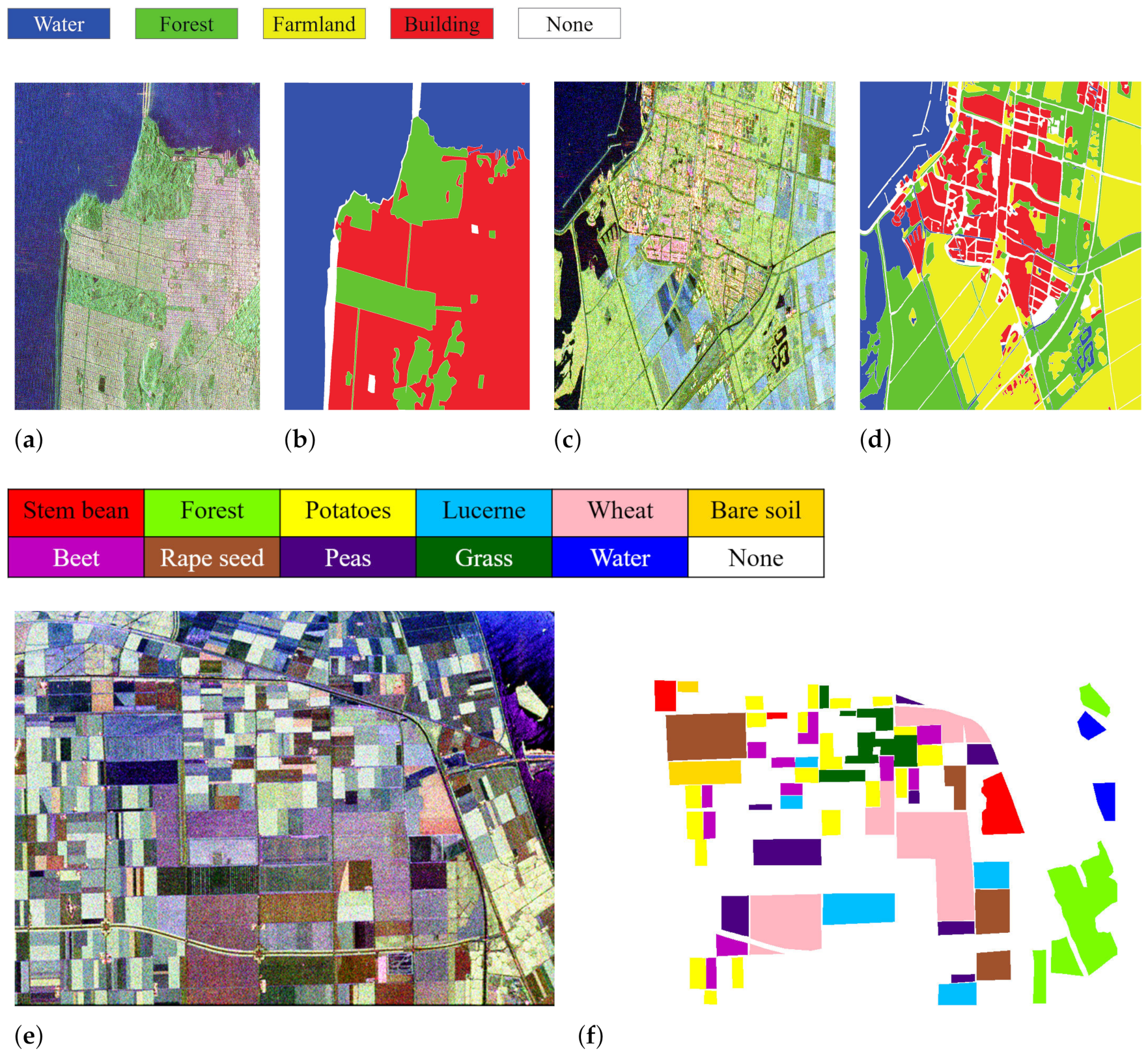
Two spaceborne PolSAR images and one airborne PolSAR image are processed to evaluate the performance of the proposed methods. The spaceborne datasets are acquired by the C-band RADARSAT-2 PolSAR system at fine quadpol mode. Rs2-Sanf data are over Sans Francisco in America, with an image size of 1600 × 1200 pixels. Rs2-Flevoland data are over Flevoland in the Netherland, with an image size of 1400 × 1200 pixels. The spatial resolution is 12 × 8 m. As-Flevoland data are the NASA/JPL AIRSAR four-look fully polarimetric data, covering Flevoland in the Netherlands. They are AIRSAR C-band data with an image size of 750 × 1024 pixels. The spatial resolution is 12 × 6 m. The RGB composite images with Pauli basis and ground-truth maps for the land-cover categories of the three PolSAR data are shown in Figure 10.
The polarimetric features are obtained from the coherency matrix. In general, each pixel in PolSAR data can be expressed in the form of the coherency matrix T 3 as follows:
T 3 = T 11 T 12 T 13 T 21 T 22 T 23 T 31 T 32 T 33
The polarimetric feature used in this paper is a nine-dimensional vector from T 3 , as shown in the following:
v = [ T 11 , T 22 , T 33 , R e ( T 12 ) , I m ( T 12 ) , R e ( T 13 ) , I m ( T 13 ) , R e ( T 23 ) , I m ( T 23 ) ]
Normalized v is applied in a multi-model triplet encoder.
For each experimental dataset, 50 labeled samples per land-cover category (about 0.003–0.007%) are randomly selected. Accuracy analysis is performed on the entire experimental image. To validate the performance of the proposed method, the four most widely used supervised classification methods including DenseNet [41], random forest (RF) [42], KNN [43] and decision tree (DT) [44] are introduced and use ten times as many labeled data for comparison.
The classification is carried out at the patch level. In comparative experiments, the patch size is 30 × 30 pixels to achieve the best classification according to experiment results shown in Figure 8. The label of the center point is considered as the category of the patch and the predicted label of each pixel is obtained by a sliding window with a step of 1. All methods take normalized T 3 as a nine-dimensional input, i.e., T 11 , T 22 , T 33 , R e ( T 12 ) , I m ( T 12 ) , R e ( T 13 ) , I m ( T 13 ) , R e ( T 23 ) , I m ( T 23 ) .
The settings of comparative experiments and ablation study are also presented as follows.
(1)
CoTraining [45]: Co-training is an improved self-training algorithm. Different classifiers are trained from different views to form a complementarity and improve the accuracy.
(2)
TriTraining [46]: A new co-training style SSL algorithm generates three classifiers from the original labeled example set. These classifiers are then refined using unlabeled examples in the tri-training process.
(3)
S3VM [24]: Semi-supervised support vector machine.
(4)
DenseNet [41]: DenseNet utilizes dense connections between layers, through dense blocks, where all layers are connected directly with each other. It can be regarded as a baseline method using the same layer as MDFGN.
(5)
RF [42]: Random forest is a commonly used machine learning algorithm.
(6)
KNN [43]: K-nearest neighbors (KNN) is a type of supervised algorithm which can be used for classification.
(7)
DT [44]: Decision tree is a type of flow chart used to visualize the decision-making process by mapping out different courses of action, as well as potential outcomes.
(8)
MDFGN without fusion strategy: The multi-level fusion strategy module is not implemented.
(9)
MDFGN without sample selection: The sample selection module is not implemented.
(10)
DenseNet with sample selection + fusion strategy: DenseNet having the same layers as MDFGN with the sample selection module and the multi-level fusion strategy module.
(11)
ResNet [47] + triplet loss: ResNet is one of the most widely used networks. Triplet loss is implemented.
The PyTorch framework is used to implement the proposed method. All the experiments were conducted on an Ubuntu 16.04 system with one 3.6 GHz 4-core i7-7700CPU, 64 GB memory and a GPU of NVIDIA GTX 1080TI. For the DenseNet and ResNet methods, the learning rate was set to 0.00005 with the decay rate set to 0.8. The performance of the proposed method is dominated by four key parameters: sampling interval ( i t v l ), number of selection loop ( N t ), initial patch size ( p s i n i ), weight of classification result ( ω ). Parameters p s i n i are set to 100, N t is set to 5. To achieve the tradeoff between sample selection efficiency and sampling density, i t v l is set to 5. To achieve the tradeoff with the noise control and detail retention, ω k is set as follows: ω 1 = 10, ω 2 = 9, ω 3 = 8, ω 4 = 7, ω 5 = 6.

4.2. Experiments and Results

In this section, the classification results of three PolSAR datasets are given. Overall accuracy (OA) and kappa coefficient are calculated to evaluate the performance of the classification. Due to the superior performance with few labeled samples, the proposed method and compared SSL methods use 50 labeled samples per category (about 0.003–0.007%), while the compared supervised methods use 500 labeled samples per category (about 0.03–0.07%).
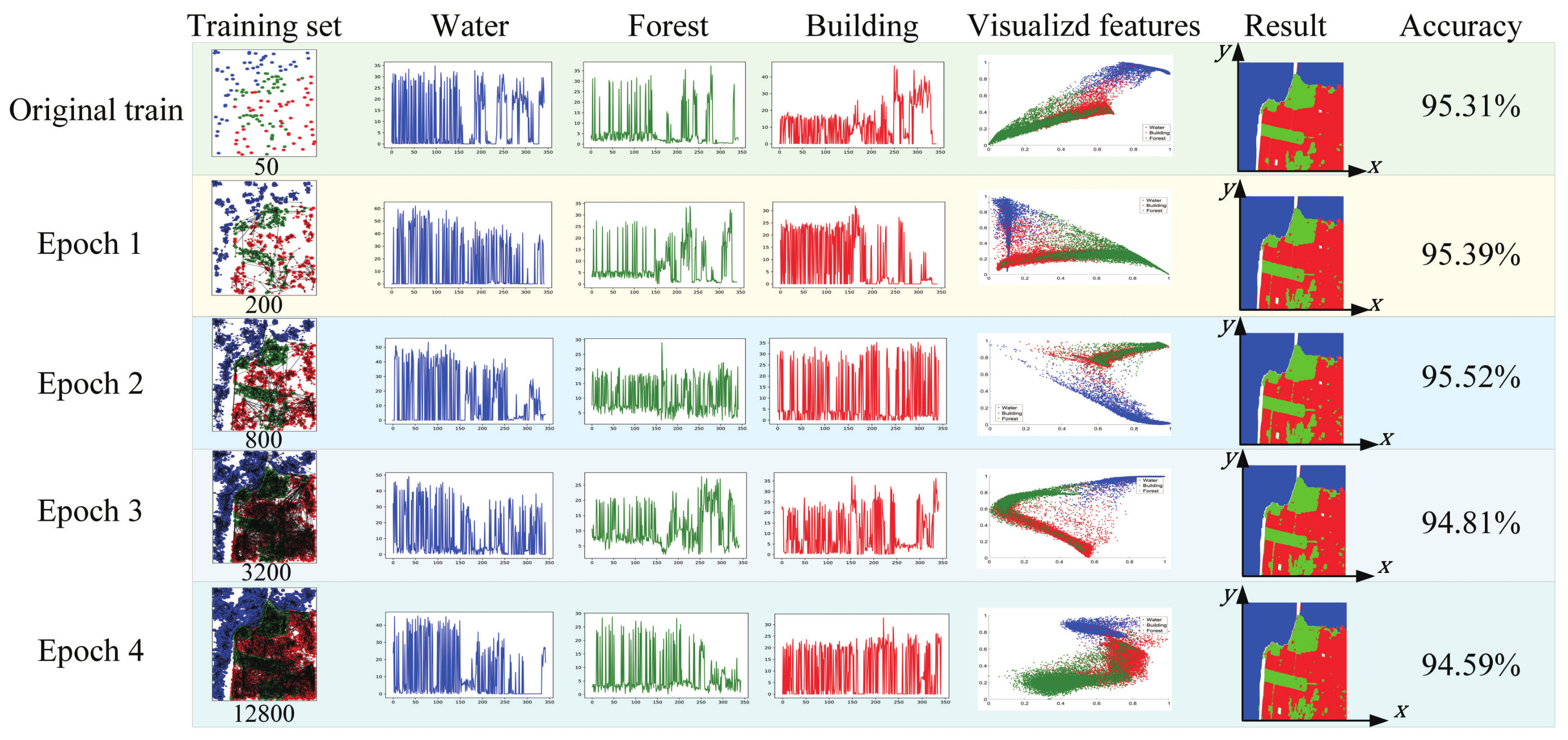
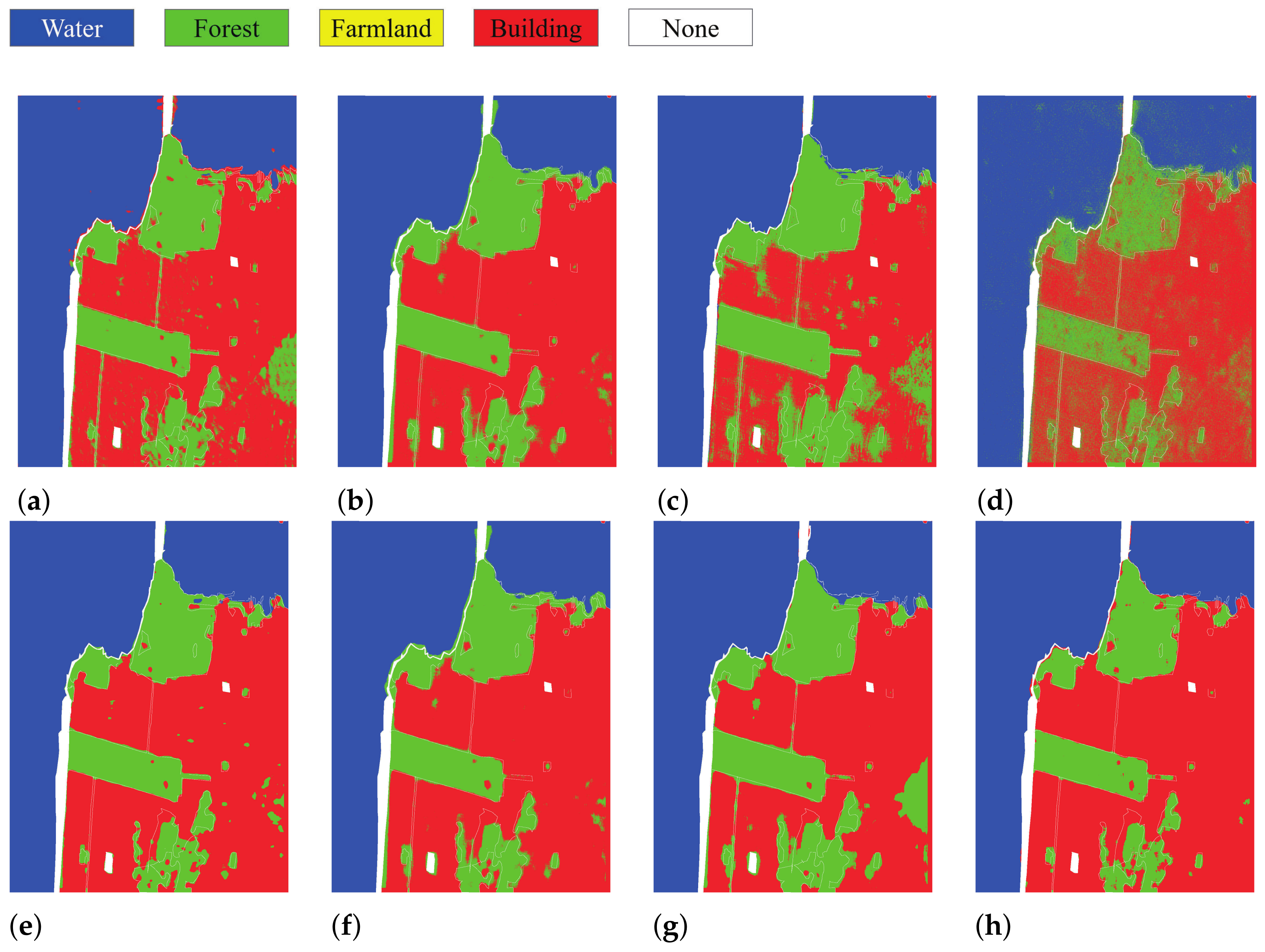
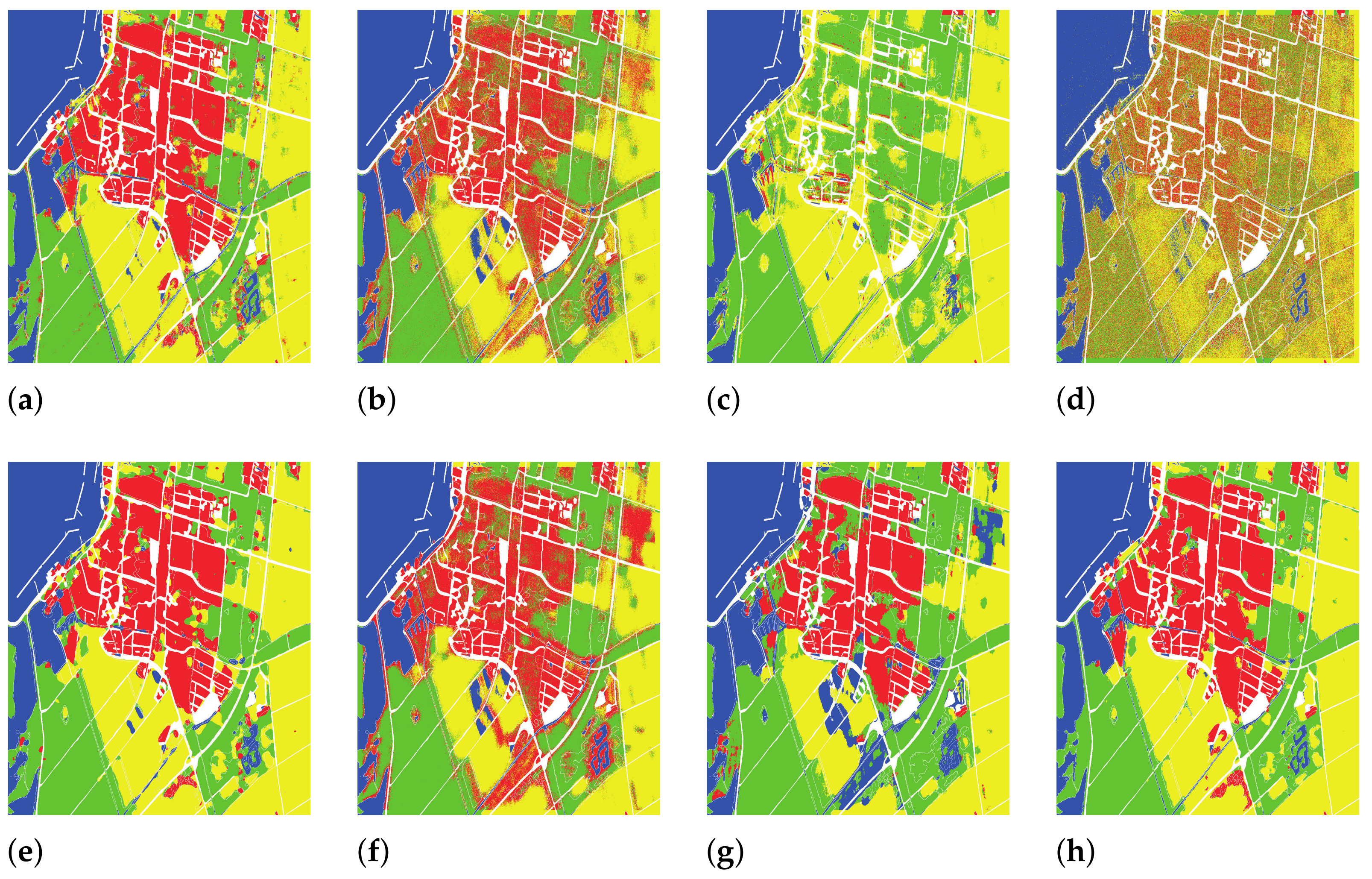
After each selecting loop, the training set is expanded to four times the last one. The central vector of each category and feature vectors using t-SNE [48] visualization demonstrate the decomposition result and the distribution of the extracted features. The training sets, central vectors, visualized features, classification results and accuracies in each selection loop are shown in Figure 11. Figure 12 shows the classification results of the Rs2-Sanf dataset and Table 1 shows the performance evaluation. The proposed method has the best classification accuracies for water and forest and the overall classification accuracy and kappa coefficient are also the highest. The following conclusions can be obtained from the results.
During the one initial training and four sample selection loops, the classification accuracy increases first because the training set is expanded and then decreases because more incorrect unlabeled samples are added into the training set. By combining the classification result of each selection loop, the final result achieves the best classification accuracy and tradeoff between detail retention and noise control, which proves the multi-level fusion strategy contributes to the accuracy.
MDFGN can obviously improve the classification performance of some land-cover types and the overall accuracy. MDFGN has the best classification accuracies for water and forest and the overall classification accuracy and kappa coefficient are also the highest. Compared with the SSL methods, the overall classification result of MDFGN is 5–7% higher than the comparative methods. Compared with the supervised methods using 10× labeled samples, the overall classification accuracy of MDFGN is 3–18% higher than the comparative supervised methods. Classification accuracy even higher than supervised methods with ten times labeled samples verifies that the capability of the proposed method for feature exploring and PolSAR data modeling is powerful.
Similarly, Figure 13 shows the classification results of the Rs2-Flevoland dataset and Table 2 shows the performance evaluation. The proposed method has the best classification accuracies for forest, farmland and building and the overall classification accuracy and kappa coefficient are also the highest. MDFGN can obviously improve the classification performance of some land-cover types and the overall classification results. Compared with the SSL methods, the overall classification accuracy of MDFGN is 6.4–15.2% higher than the comparative methods. Compared with the supervised methods using 10× labeled samples, the overall accuracy of MDFGN is 4.5–34.9% higher than the comparative supervised methods.
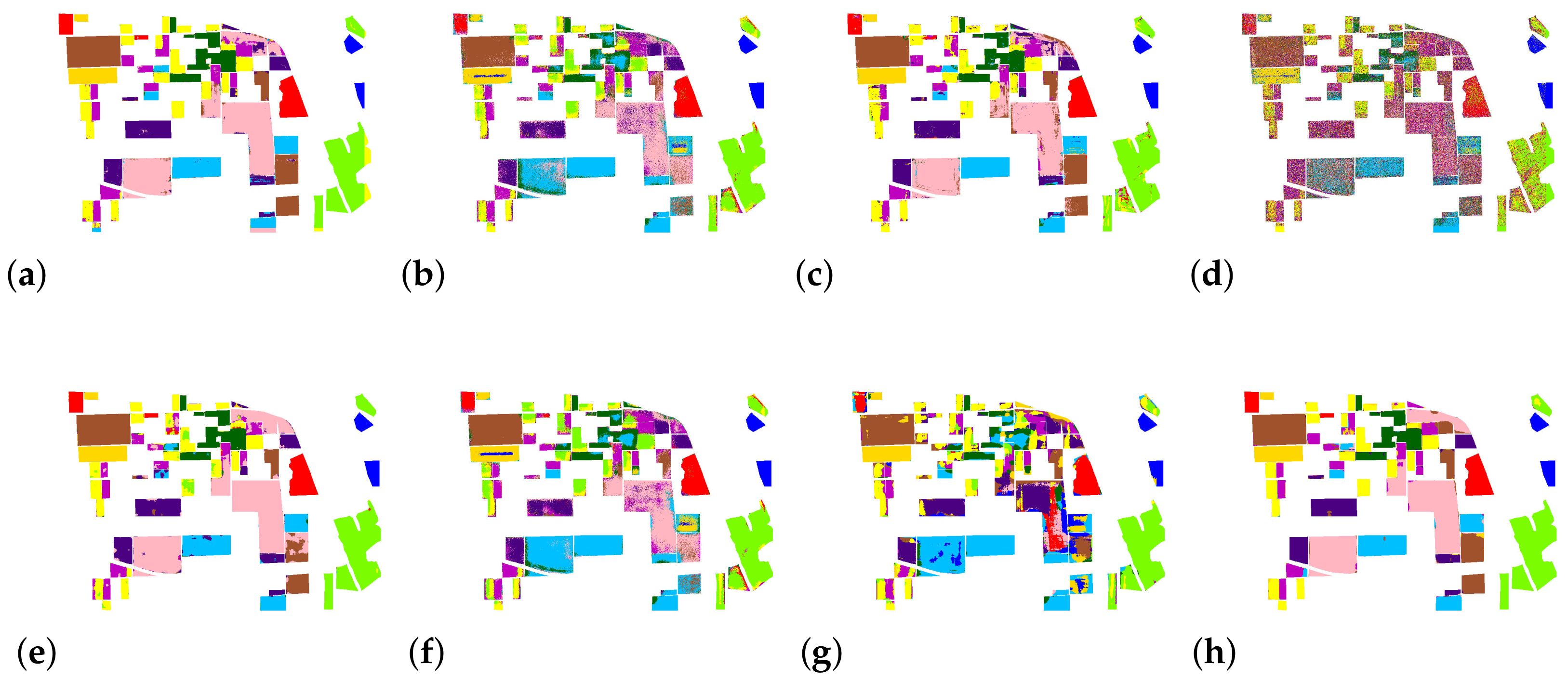
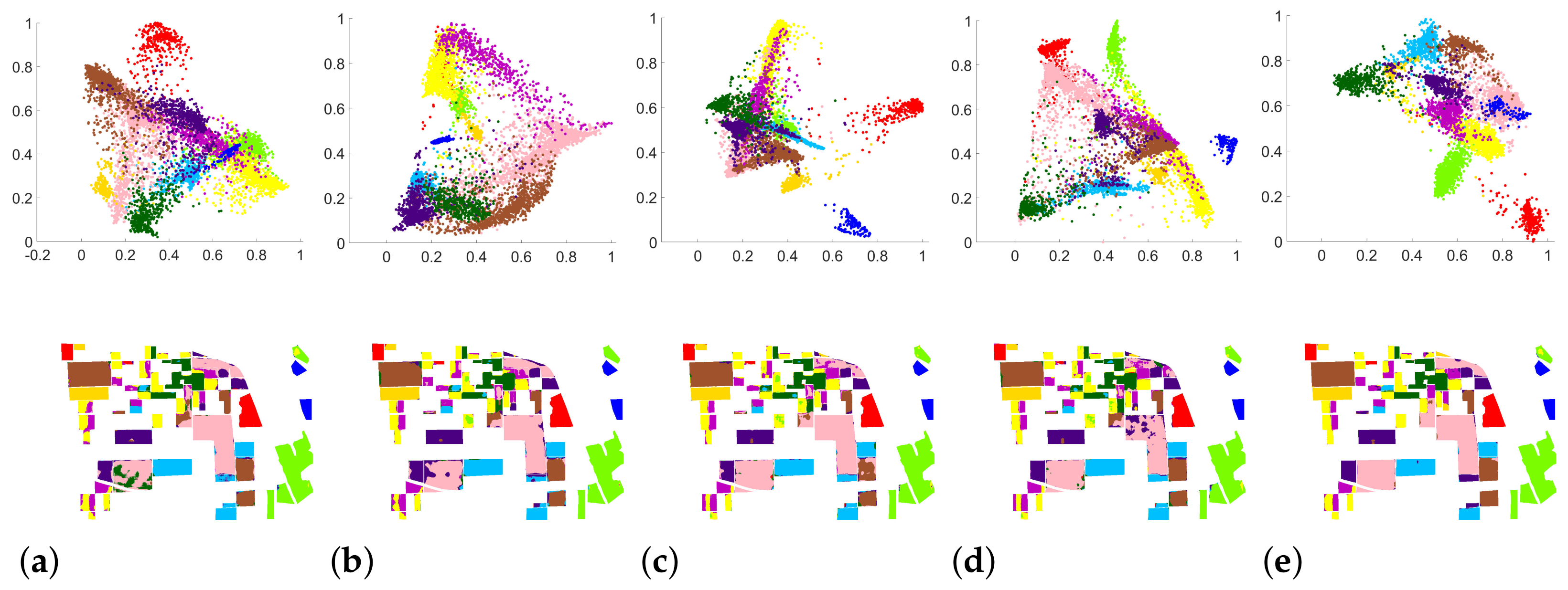
For the As-Flevoland data, Figure 14 shows the classification results and Table 3 shows the performance evaluation. The feature vectors using t-SNE [48] visualization are shown in Figure 15 and demonstrate the decomposition result and the distribution of the extracted features from 11 land-cover categories. The classification accuracies are 93.75%, 94.14%, 96.57%, 96.83% and 95.88% in each selection loop, respectively. By combining the classification result of each sample selection loop, the fused result can be obtained. The fused classification accuracy of As-Flevoland data is 98.70%, as shown in Figure 14h. The proposed method has the best classification accuracies for eight land-cover categories and the overall classification accuracy and kappa coefficient are also the highest. The proposed MDFGN significantly improves the classification accuracies of rape seed, wheat and stem bean and achieve the best classification result. As-Flevoland data contain a large number of land-cover categories and the difference of classification accuracy between the experimental methods is more obvious. The proposed method has stable and accurate classification results. The experiment result shows that the proposed method has robust and excellent performance for multi-class fine-grained classification tasks.
The three groups of experiments above show that the proposed MDFGN has robust and excellent performance for a variety of data and scenes and also shows accurate classification results for large-scale scenes and multi-class fine-grained classification tasks. MDFGN can obviously improve the classification performance of some land-cover types and the overall classification results. Compared with SSL methods using the same labeled samples, the overall classification results are 2.8–23.1% higher than the comparative methods. Compared with supervised methods using ten times the labeled samples, the overall classification results are 2.5–47.5% higher than the comparative methods. Classification results with accuracy close to or even more than 93% with few labeled samples verify that the capability of the proposed method for feature exploring and PolSAR data modeling is powerful.

5. Discussion

5.1. Analysis on the Number of Labeled Samples

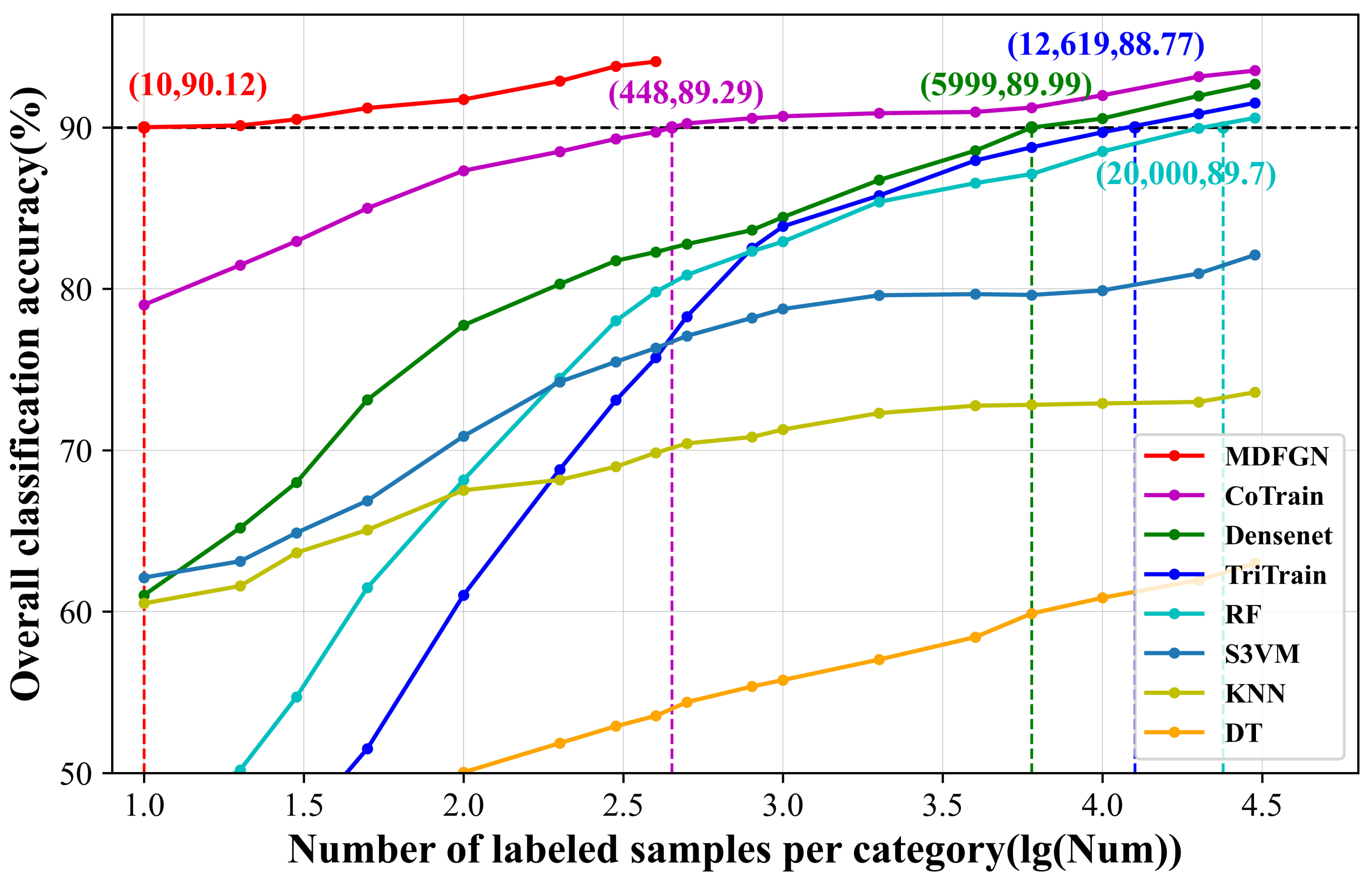
To prove the classification performance of MDFGN, we conduct the classification experiment with different labeled samples. Figure 16 demonstrates the overall accuracy curves of different models vary with the number of labeled samples. The result of Rs2-Flevoland data is presented and a similar conclusion can be obtained from the other two datasets.
As can be seen from Figure 16, the proposed MDFGN only needs 10 labeled samples for each category to reach the classification accuracy 90.12%. In contrast, co-training needs 450 labeled samples for each land-cover category, DenseNet needs 6000, the tri-training method needs 13,000 and RF needs 20,000. Even if the number of labeled samples is set to the maximum value in the experiment, the accuracy of S3VM, KNN and DT still cannot reach 90.12%.
Even though the accuracies of all methods increase with the number of labeled samples, the overall accuracy of MDFGN is much higher than other methods. The growth rate of the proposed MDFGN is lower than other methods when there are few labeled samples. The reason is that even with few labeled samples, MDFGN can select massive unlabeled samples accurately and obtain a large training set. However, other methods require sufficient labeled samples to guarantee good performance. So the accuracy is low when there are few labeled samples and the accuracy rises rapidly as the number of samples increases.
The experiment indicates that the sample selection criterion based on MDFG ensures the reliability of unlabeled samples and leads MDFGN to achieve high classification accuracy with a small number of labeled samples.

5.2. Analysis on Feature Extraction Performance

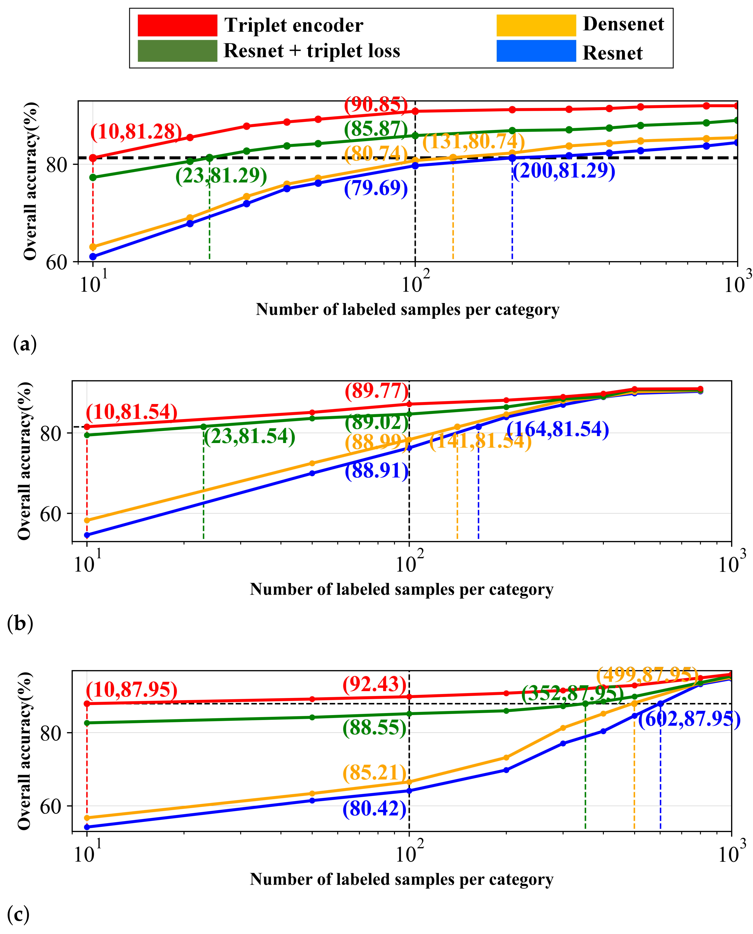
To test the feature extraction performance of the proposed encoder, we compare it with other networks. The compared networks in the experiment are ResNet, DenseNet and ResNet with triplet loss, respectively. The comparative DenseNet has the same encoding layers as the triplet encoder. The results for three data are shown in Figure 17. The following conclusions can be obtained from the experimental results.
With the same labeled samples, the triplet encoder has the highest classification accuracy. DenseNet has better performance than ResNet. The accuracy of ResNet with triplet loss is much higher than original ResNet, even better than DenseNet, which indicates that triplet loss can lead to better feature extraction performance. For Rs2-Sanf data, to reach the overall accuracy of about 81.28%, the triplet encoder uses 10 labeled samples for each category, while ResNet with triplet loss needs 23 labeled samples. In contrast, DenseNet needs 131 and ResNet needs 200 to reach the same accuracy. With the same 100 labeled samples per category, the OA of the triplet encoder is 90.85%, while ResNet with triplet loss reaches 85.87% accuracy, DenseNet reaches 80.74% accuracy and ResNet reaches 79.69% accuracy. From the results of Rs2-Flevoland and As-Flevoland data, as shown in Figure 17b,c, we can arrive at the same conclusion.
The experiment indicates that triplet loss greatly improves the performance of feature extraction. Moreover, triplet encoder has the best performance on both the feature extraction and the classification accuracy compared to other networks.

5.3. Analysis on Fusion Strategy, Sample Selection and Triplet Loss

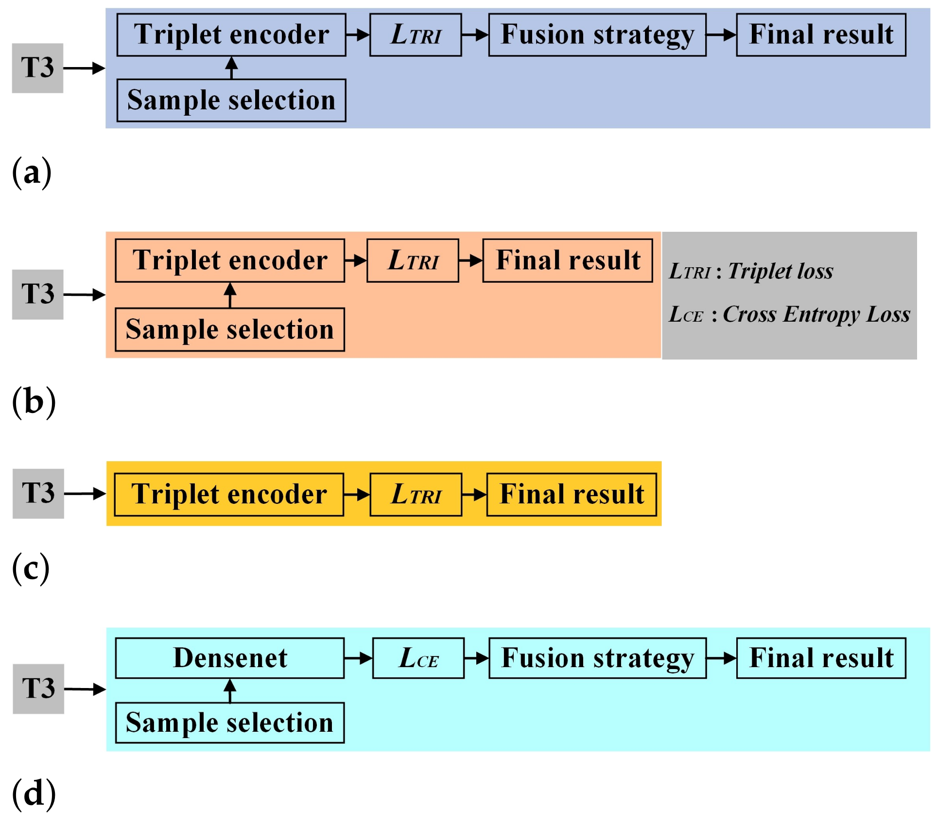
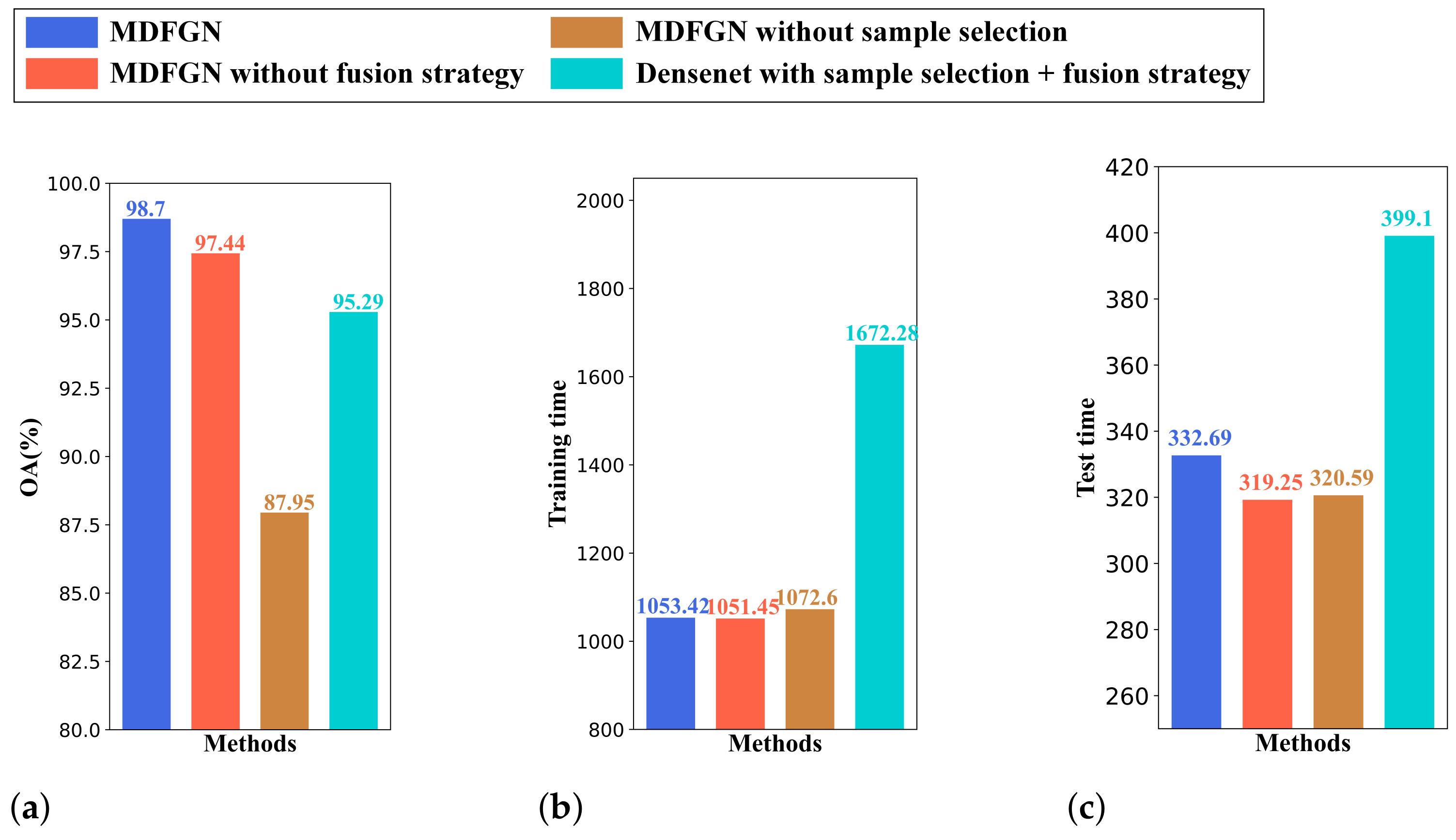
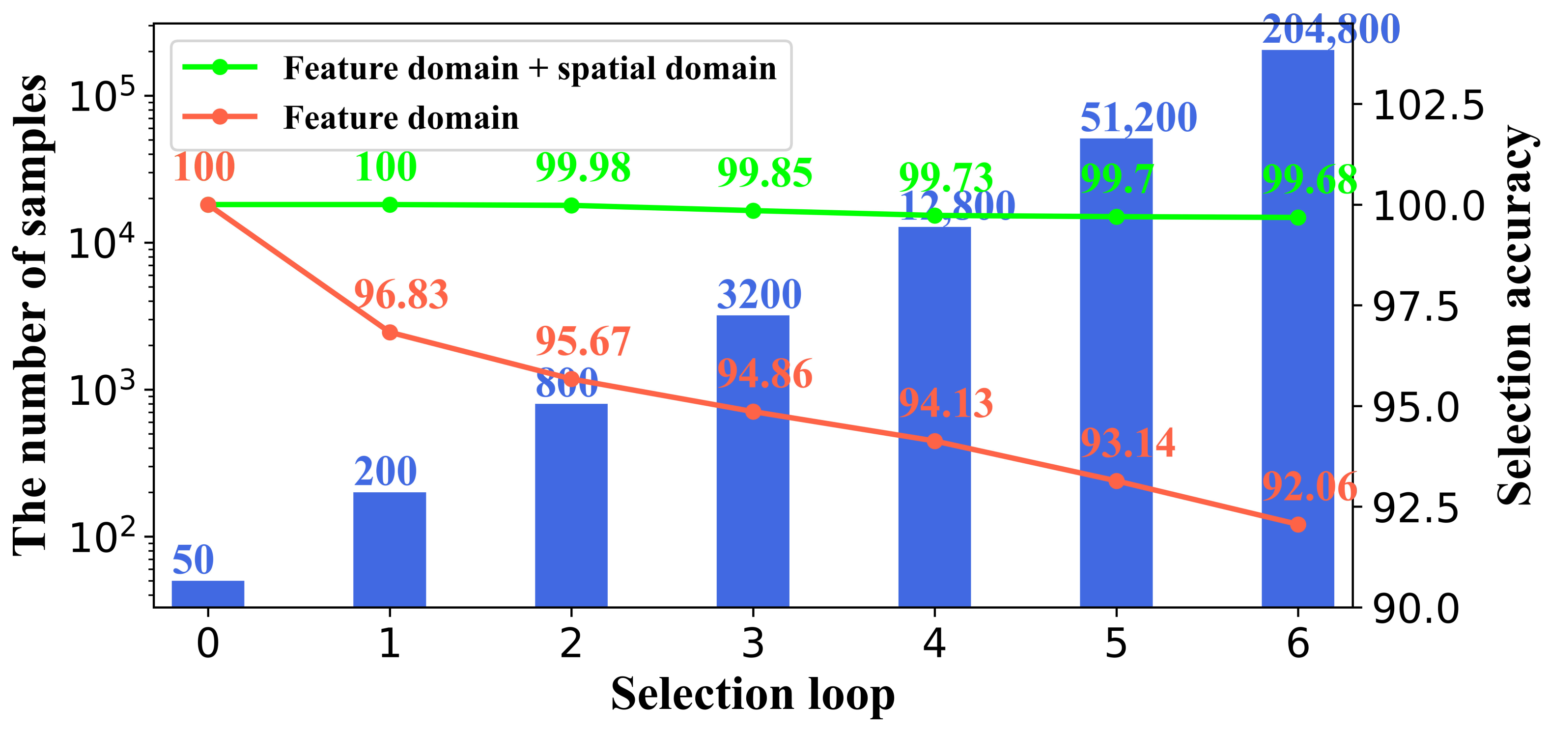
To further explore the function of the sample selection, fusion strategy and triplet loss, four models with different structures are used for the ablation study, as shown in Figure 18. The corresponding overall accuracies, training time and test time on As-Flevoland data are shown in Figure 19. The number and accuracy of selected unlabeled samples are shown in Figure 20.
The coherency matrix is the input. The triplet encoder shown in Figure 18a is utilized to extract features. The sample selection module is used for training set expansion. The loss function is triplet loss and the classification result is obtained by fusion strategy. In Figure 18b, only one classification result is obtained by the training model in the last sample selection loop. Fusion strategy is not implemented. In Figure 18c, the feature is extracted merely from the limited labeled samples without sample selection and only one classification result is obtained without the fusion strategy. In Figure 18d, DenseNet with the same encoding layers as triplet encoder is applied for feature extraction. Loss function is cross entropy loss. The selected samples are provided via MDFGN. Classification results are obtained with the fusion strategy.
As shown in Figure 19, MDFGN has the highest overall accuracy. The fusion strategy contributes 1.3% accuracy improvement. Meanwhile, training time is not changed and the extra test time consumed with respect to implementing the fusion strategy is very limited. Without sample selection, the accuracy drops 9.5%, which validates the proposal that sample selection based on MDFG improves the accuracy significantly. After implementing the triplet loss, the classification accuracy is improved by 3.4%. Meanwhile, training time and test time are shortened by 58.7% and 20.2%. So the triplet loss improves the efficiency of feature extraction and speeds up the training process and test process significantly.
As shown in Figure 20, the number of selected samples is four times that in the last selection loop. The selection accuracy of the spatial-and-feature domain is much higher than that in merely the feature domain, which validates the proposal that MDFG improves the reliability of sample selection significantly and guarantees the classification performance.
Comparison of the classification accuracy, training and test time validates that triplet loss can lead the model to improve the effectiveness of feature modeling. Sample selection can expand the training set and improve the performance of MDFGN. Meanwhile, the effect of the fusion strategy has also been verified. Advantages from these three aspects verify that every part is indispensable for PolSAR data interpretation.

5.4. Analysis of Patch Size Module

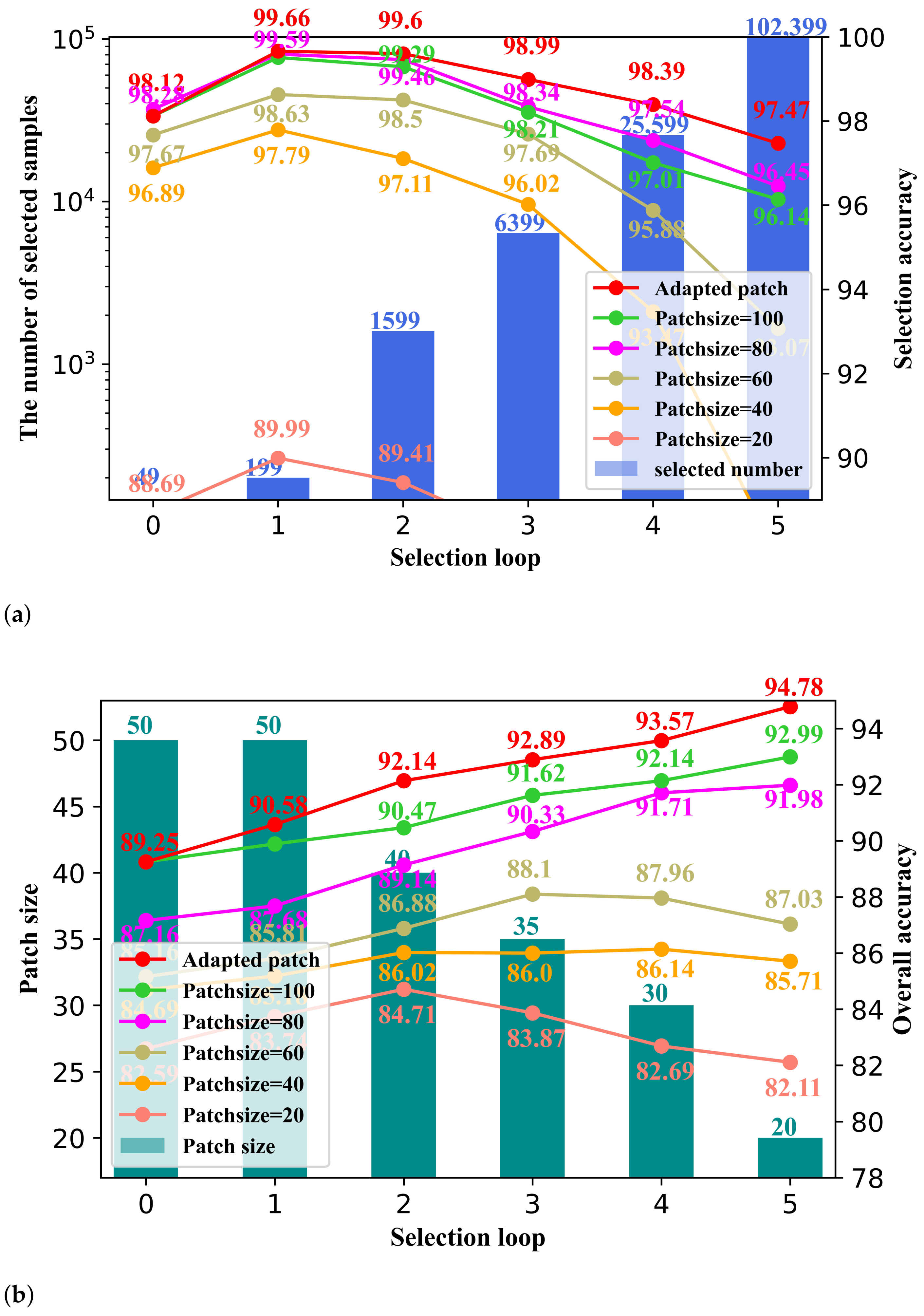
To further explore the function of the patch size module, an ablation analysis is performed on patch size. In the experiments, the adaptive patch sizes of patch size modules in each selection loop are 100 × 100, 80 × 80, 60 × 60, 40 × 40, 20 × 20, respectively. Five specific patch sizes including 100 × 100, 80 × 80, 60 × 60, 40 × 40 and 20 × 20 are tested for ablation analysis. In Figure 21a, the number of selected samples and selection accuracies at each selection loop are shown. In Figure 21b, the adaptive patch sizes for each selection loop are shown, as well as the overall accuracy for the adaptive patch size and five specific patch sizes. In comparison with other semi-supervised methods using certain patch sizes as shown in Table 2, MDFGN achieves overall accuracy for 92.99% with the same certain patch size, which is at least 2.76% higher. It verifies that MDFGN outperforms other comparative methods without the patch size module. The overall accuracy is affected not only by the number of training samples, but also by the synthetic accuracy. In comparison with other certain patch sizes, the adapted patch size achieves an overall accuracy of 94.78%, which is at least 1.79% higher. A comparison of synthetic accuracy and overall accuracy proves that the patch size module improves the effectiveness of feature modeling.

5.5. Analysis of the Number of Unlabeled Samples Connected to Labeled Samples

In the sample selection criterion, we select the unlabeled sample with the largest MDC and connect it to the labeled sample. The number of unlabeled samples connected to labeled samples (Ks) determines the pseudo-label accuracy of unlabeled samples and the number of training set samples. High accuracy and a large number of pseudo-labeled training samples lead to higher classification accuracy. With the increase in Ks, the pseudo-label accuracy decreases, but the number of training set samples increases. We chose Ks = 1, 3, 5, 8, 10 for experiments and the corresponding pseudo-label accuracy and training set sample size are shown in Figure 22. To ensure the pseudo-label accuracy and a sufficient number of training samples, the Ks is set to 3.

5.6. Analysis of the Time Cost

Table 4 shows the time consumed for training and testing of different methods on As-Flevoland data. Each model is trained with 800 epochs and the batch size is set to 64. The test is conducted on the whole PolSAR image. The proposed MDFGN has higher accuracy with less training time cost and test time cost than DenseNet and co-training. Moreover, the extra training time is very limited while the classification accuracy is improved by 12.9% compared with ResNet. Compared with KNN and S3VM, even if the training time cost is higher, the accuracy of MDFGN is at least 18.5% higher. A similar conclusion can be obtained from the other two PolSAR data.

6. Conclusions

In this paper, a novel semi-supervised classification method named multi-domain fusion graph network (MDFGN) is proposed for PolSAR image classification. The proposed MDFGN achieves high classification accuracy with few labeled samples. As a multi-model network, the proposed MDFGN extracts sufficient information from limited labeled samples. By extending the selecting domain from the feature domain to the spatial-and-feature domain, the multi-domain fusion graph leads MDFGN to obtain massive accurate unlabeled samples to expand the training set. According to the distribution of training samples, an appropriate image patch size is applied to capture both microtextures and macrotextures in the original PolSAR image. The multi-level fusion strategy is proposed to combine the results of multi-models and patch sizes to obtain accurate classification results. Experiments are carried out on Radarsat-2 and AIRSAR PolSAR images. With few labeled samples (about 0.003–0.007%), the overall accuracy of the proposed method ranges between 94.78% and 99.24%. The average accuracy is 5% higher than that of the classical semi-supervised methods and even 4.5% higher than that of the classical supervised methods with ten times the labeled samples.

Author Contributions

Conceptualization, R.T.; methodology, R.T.; software, R.T.; validation, R.T.; formal analysis, R.T.; investigation, R.T.; resources, R.T., F.P. and R.Y.; data curation, R.T.; writing—original draft preparation, R.T.; writing—review and editing, R.T.; visualization, R.T.; supervision, Z.X. and X.X. All authors have read and agreed to the published version of the manuscript.

Funding

This research was funded by National Natural Science Foundation of China OF FUNDER grant number 62071336.

Data Availability Statement

All data included in this study are available upon request by contact with the corresponding author.

Conflicts of Interest

The authors declare no conflict of interest.

References

  1. Marmanis, D.; Datcu, M.; Esch, T.; Stilla, U. Deep learning earth observation classification using ImageNet pretrained networks. IEEE Geosci. Remote Sens. Lett. 2015, 13, 105–109. [Google Scholar] [CrossRef] [Green Version]
  2. Zhu, X.X.; Tuia, D.; Mou, L.; Xia, G.S.; Zhang, L.; Xu, F.; Fraundorfer, F. Deep learning in remote sensing: A comprehensive review and list of resources. IEEE Geosci. Remote Sens. Mag. 2017, 5, 8–36. [Google Scholar] [CrossRef] [Green Version]
  3. Desai, A.; Xu, Z.; Gupta, M.; Chandran, A.; Vial-Aussavy, A.; Shrivastava, A. Raw Nav-merge Seismic Data to Subsurface Properties with MLP based Multi-Modal Information Unscrambler. Adv. Neural Inf. Process. Syst. 2021, 34, 8740–8752. [Google Scholar]
  4. Wang, L.; Xu, X.; Yu, Y.; Yang, R.; Gui, R.; Xu, Z.; Pu, F. SAR-to-Optical Image Translation Using Supervised Cycle-Consistent Adversarial Networks. IEEE Access 2019, 7, 129136–129149. [Google Scholar] [CrossRef]
  5. Dong, H.; Xu, X.; Sui, H.; Xu, F.; Liu, J. Copula-Based Joint Statistical Model for Polarimetric Features and Its Application in PolSAR Image Classification. IEEE Trans. Geosci. Remote Sens. 2017, 55, 5777–5789. [Google Scholar] [CrossRef]
  6. Yang, R.; Xu, X.; Gui, R.; Xu, Z.; Pu, F. Composite Sequential Network with POA Attention for PolSAR Image Analysis. IEEE Trans. Geosci. Remote Sens. 2022, 60, 1–15. [Google Scholar] [CrossRef]
  7. Zhou, Y.; Wang, H.; Xu, F.; Jin, Y. Polarimetric SAR Image Classification Using Deep Convolutional Neural Networks. IEEE Geosci. Remote Sens. Lett. 2016, 13, 1935–1939. [Google Scholar] [CrossRef]
  8. Gao, F.; Huang, T.; Wang, J.; Sun, J. Dual-Branch Deep Convolution Neural Network for Polarimetric SAR Image Classification. Appl. Sci. 2017, 7, 447. [Google Scholar] [CrossRef] [Green Version]
  9. Zhang, Z.; Wang, H.; Xu, F.; Jin, Y.Q. Complex-Valued Convolutional Neural Network and Its Application in Polarimetric SAR Image Classification. IEEE Trans. Geosci. Remote Sens. 2017, 55, 7177–7188. [Google Scholar] [CrossRef]
  10. Li, Y.; Chen, Y.; Liu, G.; Jiao, L. A Novel Deep Fully Convolutional Network for PolSAR Image Classification. Remote Sens. 2018, 10, 1984–2001. [Google Scholar] [CrossRef] [Green Version]
  11. Cao, Y.; Wu, Y.; Zhang, P.; Liang, W.; Li, M. Pixel-Wise PolSAR Image Classification via a Novel Complex-Valued Deep Fully Convolutional Network. Remote Sens. 2019, 11, 2653–2682. [Google Scholar] [CrossRef]
  12. Chen, Y.; Li, Y.; Jiao, L.; Peng, C.; Zhang, X.; Shang, R. Adversarial Reconstruction-Classification Networks for PolSAR Image Classification. Remote Sens. 2019, 11, 415–419. [Google Scholar] [CrossRef] [Green Version]
  13. Mullissa, A.G.; Persello, C.; Stein, A. PolSARNet: A Deep Fully Convolutional Network for Polarimetric SAR Image Classification. IEEE J. Sel. Top. Appl. Earth Obs. Remote Sens. 2019, 12, 5300–5309. [Google Scholar] [CrossRef]
  14. Mohammadimanesh, F.; Salehi, B.; Mandianpari, M.; Gill, E.; Molinier, M. A new fully convolutional neural network for semantic segmentation of polarimetric SAR imagery in complex land cover ecosystem. ISPRS J. Photogramm. Remote Sens. 2019, 151, 223–236. [Google Scholar] [CrossRef]
  15. He, C.; Tu, M.; Xiong, D.; Liao, M. Nonlinear manifold learning integrated with fully convolutional networks for polSAR image classification. Remote Sens. 2020, 12, 655. [Google Scholar] [CrossRef] [Green Version]
  16. Zhao, F.; Tian, M.; Xie, W.; Liu, H. A New Parallel Dual-Channel Fully Convolutional Network via Semi-Supervised FCM for PolSAR Image Classification. IEEE J. Sel. Top. Appl. Earth Obs. Remote Sens. 2020, 13, 4493–4505. [Google Scholar] [CrossRef]
  17. Wang, Y.; Gao, L.; Gao, Y.; Li, X. A new graph-based semi-supervised method for surface defect classification. Robot. Comput. -Integr. Manuf. 2021, 68, 102083. [Google Scholar] [CrossRef]
  18. Du, Y.; Liu, F.; Qiu, J.; Buss, M. A Semi-Supervised Learning Approach for Identification of Piecewise Affine Systems. IEEE Trans. Circuits Syst. I Regul. Pap. 2020, 67, 3521–3532. [Google Scholar] [CrossRef]
  19. Wang, S.; Guo, Y.; Hua, W.; Liu, X.; Song, G.; Hou, B.; Jiao, L. Semi-Supervised PolSAR Image Classification Based on Improved Tri-Training With a Minimum Spanning Tree. IEEE Trans. Geosci. Remote Sens. 2020, 58, 8583–8597. [Google Scholar] [CrossRef]
  20. Du, L.; Wang, Y.; Xie, W. A semi-supervised method for sar target discrimination based on co-training. In Proceedings of the 2019 IEEE International Geoscience and Remote Sensing Symposium (IGARSS 2019), Yokohama, Japan, 28 July–2 August 2019; pp. 9482–9485. [Google Scholar]
  21. Emadi, M.; Tanha, J.; Shiri, M.E.; Aghdam, M.H. A Selection Metric for semi-supervised learning based on neighborhood construction. Inf. Process. Manag. 2021, 58, 102444. [Google Scholar] [CrossRef]
  22. Ding, Y.; Zhao, X.; Zhang, Z.; Cai, W.; Yang, N.; Zhan, Y. Semi-Supervised Locality Preserving Dense Graph Neural Network With ARMA Filters and Context-Aware Learning for Hyperspectral Image Classification. IEEE Trans. Geosci. Remote Sens. 2022, 60, 5511812. [Google Scholar] [CrossRef]
  23. He, Z.; Liu, H.; Wang, Y.; Hu, J. Generative Adversarial Networks-Based Semi-Supervised Learning for Hyperspectral Image Classification. Remote Sens. 2017, 9, 1042. [Google Scholar] [CrossRef] [Green Version]
  24. Li, Y.; Li, H.; Guan, C.; Chin, Z. A self-training semi-supervised support vector machine algorithm and its applications in brain computer interface. In Proceedings of the International Conference on Acoustics Speech and Signal Processing ICASSP 2007, Toronto, ON, Canada, 7–13 May 2007; pp. 385–388. [Google Scholar]
  25. Jean, N.; Wang, S.; Samar, A.; Azzari, G.; Lobell, D.; Ermon, S. Tile2Vec: Unsupervised Representation Learning for Spatially Distributed Data. Assoc. Adv. Artif. Intell. 2019, 33, 3967–3974. [Google Scholar] [CrossRef] [Green Version]
  26. Malkov, Y.A.; Yashunin, D.A. Efficient and Robust Approximate Nearest Neighbor Search Using Hierarchical Navigable Small World Graphs. IEEE Trans. Pattern Anal. Mach. Intell. 2020, 42, 824–836. [Google Scholar] [CrossRef] [PubMed] [Green Version]
  27. Hoffer, E.; Ailon, N. Deep Metric Learning Using Triplet Network. Lect. Notes Comput. Sci. 2015, 9370, 84–92. [Google Scholar]
  28. Gong, Z.; Zhong, P.; Yu, Y.; Hu, W. Diversity-Promoting Deep Structural Metric Learning for Remote Sensing Scene Classification. IEEE Trans. Geosci. Remote Sens. 2018, 56, 371–390. [Google Scholar] [CrossRef]
  29. Yang, R.; Xu, X.; Xu, Z.; Dong, H.; Gui, R.; Pu, F. Dynamic Fractal Texture Analysis for PolSAR Land Cover Classification. IEEE Trans. Geosci. Remote Sens. 2019, 57, 5991–6002. [Google Scholar] [CrossRef]
  30. Zhao, Y.; Cheung, Y.m.; You, X.; Peng, Q.; Peng, J.; Yuan, P.; Shi, Y. Hyperspectral Image Classification via Spatial Window-Based Multiview Intact Feature Learning. IEEE Trans. Geosci. Remote Sens. 2021, 59, 2294–2306. [Google Scholar] [CrossRef]
  31. Ding, Y.; Zhao, X.; Zhang, Z.; Cai, W.; Yang, N. Graph Sample and Aggregate-Attention Network for Hyperspectral Image Classification. IEEE Geosci. Remote Sens. Lett. 2022, 19, 5504205. [Google Scholar] [CrossRef]
  32. Ding, Y.; Zhang, Z.; Zhao, X.; Hong, D.; Cai, W.; Yu, C.; Yang, N.; Cai, W. Multi-feature fusion: Graph neural network and CNN combining for hyperspectral image classification. Neurocomputing 2022, 501, 246–257. [Google Scholar] [CrossRef]
  33. Ding, Y.; Zhao, X.; Zhang, Z.; Cai, W.; Yang, N. Multiscale Graph Sample and Aggregate Network With Context-Aware Learning for Hyperspectral Image Classification. IEEE J. Sel. Top. Appl. Earth Obs. Remote Sens. 2021, 14, 4561–4572. [Google Scholar] [CrossRef]
  34. Cao, Y.; Liu, J.; Qi, H.; Gui, J.; Li, K.; Ye, J.; Liu, C. Scalable Distributed Hashing for Approximate Nearest Neighbor Search. IEEE Trans. Image Process. 2022, 31, 472–484. [Google Scholar] [CrossRef]
  35. Ponomarenko, A.; Mal’kov, Y.; Logvinov, A.; Krylov, V. Approximate Nearest Neighbor Search Small World Approach. In Proceedings of the International Conference on Information and Communication Technologies & Applications, Azerbaijan, Baku, 12–14 October 2011; pp. 40–45. [Google Scholar]
  36. Franceschetti, M.; Meester, R. Navigation in small-world networks: A scale-free continuum model. J. Appl. Probab. 2006, 43, 1173–1180. [Google Scholar] [CrossRef] [Green Version]
  37. Boguna, M.; Krioukov, D.; Claffy, K.C. Navigability of complex networks. Nat. Phys. 2009, 5, 74–80. [Google Scholar] [CrossRef] [Green Version]
  38. Kang, J.; Fernandez-Beltran, R.; Ye, Z.; Tong, X.; Ghamisi, P.; Plaza, A. Deep Metric Learning Based on Scalable Neighborhood Components for Remote Sensing Scene Characterization. IEEE Trans. Geosci. Remote Sens. 2020, 58, 8905–8918. [Google Scholar] [CrossRef]
  39. Yan, L.; Zhu, R.; Mo, N.; Liu, Y. Cross-Domain Distance Metric Learning Framework With Limited Target Samples for Scene Classification of Aerial Images. IEEE Trans. Geosci. Remote Sens. 2019, 57, 3840–3857. [Google Scholar] [CrossRef]
  40. Penatti, O.A.B.; Nogueira, K.; dos Santos, J.A. Do Deep Features Generalize from Everyday Objects to Remote Sensing and Aerial Scenes Domains? In Proceedings of the 2015 IEEE Conference on Computer Vision and Pattern Recognition Workshops (CVPRW), Boston, MA, USA, 7–12 June 2015.
  41. Li, G.; Zhang, M.; Li, J.; Lv, F.; Tong, G. Efficient densely connected convolutional neural networks. Pattern Recognit. 2021, 109, 107610. [Google Scholar] [CrossRef]
  42. Haensch, R.; Hellwich, O. Classification of PolSAR Images by Stacked Random Forests. ISPRS Int. J. Geo-Inf. 2018, 7, 74. [Google Scholar] [CrossRef] [Green Version]
  43. Isuhuaylas, L.A.V.; Hirata, Y.; Ventura Santos, L.C.; Serrudo Torobeo, N. Natural Forest Mapping in the Andes (Peru): A Comparison of the Performance of Machine-Learning Algorithms. Remote Sens. 2018, 10, 782. [Google Scholar] [CrossRef] [Green Version]
  44. Berhane, T.M.; Lane, C.R.; Wu, Q.; Autrey, B.C.; Anenkhonov, O.A.; Chepinoga, V.V.; Liu, H. Decision-Tree, Rule-Based and Random Forest Classification of High-Resolution Multispectral Imagery for Wetland Mapping and Inventory. Remote Sens. 2018, 10, 580. [Google Scholar] [CrossRef] [Green Version]
  45. Lu, X.; Zhang, J.; Li, T.; Zhang, Y. Incorporating Diversity into Self-Learning for Synergetic Classification of Hyperspectral and Panchromatic Images. Remote Sens. 2016, 8, 804. [Google Scholar] [CrossRef] [Green Version]
  46. Zhou, Z.; Li, M. Tri-training: Exploiting unlabeled data using three classifiers. IEEE Trans. Knowl. Data Eng. 2005, 17, 1529–1541. [Google Scholar] [CrossRef]
  47. He, K.; Zhang, X.; Ren, S.; Sun, J. Deep Residual Learning for Image Recognition. In Proceedings of the 2016 IEEE Conference on Computer Vision and Pattern Recognition (CVPR), Las Vegas, NV, USA, 27–30 June 2016; pp. 770–778. [Google Scholar]
  48. van der Maaten, L.; Hinton, G. Visualizing Data using t-SNE. J. Mach. Learn. Res. 2008, 9, 2579–2605. [Google Scholar]
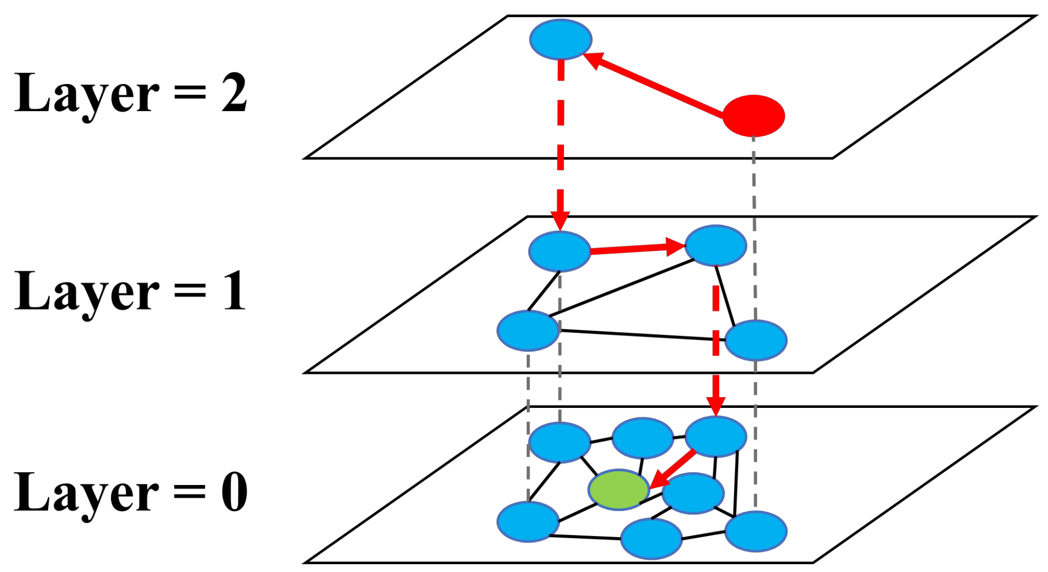
Figure 1. Illustration of HNSW. Data points are vertices and the similarity between points are edges. The search starts from an element from the top layer (shown red point). Red arrows show direction of the searching algorithm from the entry point to the query point (shown green point).
Remotesensing 15 00160 g001
Figure 2. Triplet network.
Remotesensing 15 00160 g002
Figure 3. Architecture of the proposed multi-domain fusion graph network.
Remotesensing 15 00160 g003
Figure 4. Multi-domain fusion graph.
Remotesensing 15 00160 g004
Figure 5. Sample selection. (a) Regions of Rs2-Sanf. Each region is separated by other land-cover categories. (b) First training set of labeled samples. (cg) Selected samples after one-five selection loops. The small light-colored points are the selected unlabeled samples which are connected to the labeled samples represented by the large dark-colored points.
Remotesensing 15 00160 g005
Figure 6. Multi-model Triplet Encoder.
Remotesensing 15 00160 g006
Figure 7. (a) Feature extraction process of deep learning network. (b) Ground truth map. (cg) respectively correspond to the classification result with ResNet on Rs2-Sanf data when patch size = 5, 10, 30, 50, 100.
Remotesensing 15 00160 g007
Figure 8. The overall classification accuracy varies with patch sizes when there are different labeled samples applying ResNet on Rs2-Sanf data.
Remotesensing 15 00160 g008
Figure 9. Classification Process.
Remotesensing 15 00160 g009
Figure 10. Pauli-based RGB images and manually labeled ground truth maps of the experimental data. (a,b) Rs2-Sanf data; (c,d) Rs2-Flevoland data; (e,f) As-Flevoland data.
Remotesensing 15 00160 g010
Figure 11. Training process and result of each selection loop on Rs2-Sanf. Training set, central vector of each land-cover category, visualization features of 342-D features vector visualized by t-SNE, classification result and accuracy.
Remotesensing 15 00160 g011
Figure 12. Classification results on Rs2-Sanf. (a) DenseNet. (b) RF. (c) KNN. (d) DT. (e) Co-training. (f) Tri-training. (g) S3VM. (h) MDFGN.
Remotesensing 15 00160 g012
Figure 13. Classification results on Rs2-Flevoland. (a) DenseNet. (b) RF. (c) KNN. (d) DT. (e) Co-training. (f) Tri-training. (g) S3VM. (h) MDFGN.
Remotesensing 15 00160 g013
Figure 14. (a) DenseNet. (b) RF. (c) KNN. (d) DT. (e) Co-training. (f) Tri-training. (g) S3VM. (h) MDFGN.
Remotesensing 15 00160 g014
Figure 15. Visualization features of 342-D feature vector and classification results of each loop on AIR-Flev I. (a) Origin train. (b) Epoch 1. (c) Epoch 2. (d) Epoch 3. (e) Epoch 4.
Remotesensing 15 00160 g015
Figure 16. Overall accuracies of different methods varying with the number of labeled samples for the As-Flevoland data.
Remotesensing 15 00160 g016
Figure 17. Overall accuracies vary with the number of labeled samples of the three experimental data. (a) Rs2-Sanf data; (b) Rs2-Flevoland data; (c) As-Flevoland data.
Remotesensing 15 00160 g017
Figure 18. Model structures of 4 groups of ablation studies. (a) MDFGN; (b) MDFGN without fusion strategy; (c) MDFGN without sample selection; (d) DenseNet with sample selection + fusion strategy.
Remotesensing 15 00160 g018
Figure 19. Overall accuracies, training time and test time of different networks on AIR-Flev data. (a) Overall accuracy; (b) Training time; (c) Test time.
Remotesensing 15 00160 g019
Figure 20. The number of training samples and the accuracy of the selected samples.
Remotesensing 15 00160 g020
Figure 21. Ablation study on the effect of the patch size module. (a) The number of selected samples and selection accuracy for each selection loop; (b) The adaptive patch size in each selection loop and overall accuracy.
Remotesensing 15 00160 g021
Figure 22. The number and the pseudo-label accuracy of the training set with different numbers of unlabeled samples connected to labeled samples (Ks) on Rs2-Sanf Data.
Remotesensing 15 00160 g022
Table 1. Classification accuracy (%) on Rs2-Sanf Data.
Classification Method   Water  Forest  Building  OA  Kappa 
CoTraining99.2989.9292.1393.9090.35
TriTraining98.0492.9391.4694.8692.10
S3VM99.7287.6394.2293.6590.33
MDFGN99.7599.8189.4998.1697.12
DenseNet99.6994.1893.4696.3494.35
RF98.3591.7091.7494.4991.55
KNN99.6978.5796.1890.0385.07
DT95.1581.0077.2286.3779.35
Table 2. Classification accuracy (%) for Rs2-Flevoland data.
Class Co-
Training 
 Tri-
Training 
 S3VM  DenseNet  RF  KNN  DT MDFGN 
Water97.6395.6787.5795.7196.1795.5492.1796.42
Forest84.0489.8489.8488.3584.9787.1551.7892.16
Building80.5882.4879.3792.0186.8291.4756.6492.79
Farmland90.5887.3562.3287.7884.608.0850.5496.85
OA87.3988.4179.6290.2387.3872.8159.8894.78
Kappa83.5584.2272.7686.7882.8662.2145.7893.32
Table 3. Classification accuracy (%) for AIR-Flev data.
Class Co-
Training 
 Tri-
Training 
 S3VM  DenseNet  RF  KNN  DT MDFGN 
Stem bean97.8688.8279.4695.8983.9895.2652.4299.67
Forest99.0286.0188.5699.4685.1789.1656.2099.82
Potatoes96.8440.9173.4197.1557.9891.5840.3192.61
Lucerne95.9978.5677.7196.6983.2995.5756.0897.79
Wheat90.9145.4508.9591.0950.3384.3928.2292.34
Bare soil98.9788.2197.9299.9689.2499.5175.6399.93
Beet96.8778.5952.0795.7868.6688.4234.1290.22
Rape seed92.4966.1068.0390.0963.3195.5550.9595.97
Peas93.9257.6456.0892.1958.2392.1331.5887.67
Grass97.9674.8560.4098.1765.3395.0645.4498.07
Water98.3899.6896.2894.9099.8594.6991.0199.79
OA95.7991.1789.3696.2091.6093.7485.8798.70
Kappa95.9179.7175.6195.6680.6994.8067.5597.00
Table 4. Time consumed (s) for training and validation of different methods.
Classification MethodOATraining Time (800 Epochs)Test Time
DenseNet94.521577.85386.21
ResNet85.39868.44372.25
KNN79.79-239.64
CoTraining89.506519.97352.4
S3VM55.19228.611.29
MDFGN98.301053.42319.25
Disclaimer/Publisher’s Note: The statements, opinions and data contained in all publications are solely those of the individual author(s) and contributor(s) and not of MDPI and/or the editor(s). MDPI and/or the editor(s) disclaim responsibility for any injury to people or property resulting from any ideas, methods, instructions or products referred to in the content.