Evaluation of Numerous Kinetic Energy-Rainfall Intensity Equations Using Disdrometer Data

Abstract

Calculating rainfall erosivity, which is the capacity of rainfall to dislodge soil particles and cause erosion, requires the measurement of the rainfall kinetic energy (KE). Direct measurement of KE has its own challenges, owing to the high cost and complexity of the measuring instruments involved. Consequently, the KE is often approximated using empirical equations derived from rainfall intensity (I_r) inputs in the absence of such instruments. However, the KE–I_r equations strongly depend on local climate patterns and measurement methods. Therefore, this study aims to compare and evaluate the efficacy of 27 KE–I_r equations with observed data. Based on a re-analysis, we also propose an exponential KE–I_r equation for the entire Korean site, and the spatial distribution of its parameter in the equation is also discussed. In this investigation, we used an optical disdrometer (OTT Parsivel²) to gather data in Sangju City (Korea) between June 2020 and December 2021. The outputs of this study are shown as follows: (1) The statistically most accurate estimates of KE expenditure and KE content in Sangju City are obtained using power-law equations given by Sanchez-Moreno et al. and exponential equations published by Lee and Won, respectively. (2) The suggested KE–I_r equation applied to the entire Korean site exhibits a comparable general correlation with the observed data. The parameter maps indicate a high variance in geography.

1. Introduction

In nature, soil provides a variety of essential functions that aid in the maintenance of an environment that is resistant to drought [1], floods [2], and wildfires [3]. The increasing extreme rainfall events due to climate change [4] and their harmful effects are emerging issues in contemporary civilizations, which are strongly connected with surface soil erosion [5]. Water-induced soil erosion causes significant environmental and agricultural harm during severe precipitation events [6]. Therefore, it is necessary to understand the soil erosion processes.

Soil erosion by water involves separation by rainfall impact [7] and the movement of soil particles by surface runoff agents [8]. Splash erosion, the first step in water-induced soil loss, has been acknowledged to be a crucial stage in initiating surface soil erosion [9]. The relationship between rainfall intensity (I_r) and rainsplash erosion under field conditions has been comprehensively investigated [10]. Raindrops release kinetic energy (KE) when they strike the ground, forcing soil particles to become airborne and triggering rainsplash erosion [11]. The KE of rainfall includes two distinct types: kinetic energy expenditure (KE_exp; J m⁻²h⁻¹) and kinetic energy content (KE_con; J m⁻²mm⁻¹). The former is the rate at which the KE is spent per unit area over a certain period, and the latter is defined as the KE per unit area per unit depth. These two types of KE are connected by I_r in the following formulation: KE_con = KE_exp/I_r.

Owing to the expense and complexity of the procedure, direct measurements of KE have been terminated since the first attempt by Madden et al. [12]. Consequently, empirical equations are a replacement for estimating KE from I_r, which is easy to collect. Precise measurement of the mass and velocity of raindrops is required for accurate determination of the KE, and there are many ways to measure raindrop properties. Early research from the 1900s sought to measure raindrop size and velocity using manual measuring methods [13]. Since 1960, acoustic/piezoelectric sensors have been employed to measure the size of raindrops, allowing for automated data collection and a significant reduction in labor. With the introduction of technical and electrical advancements, laser-based equipments (i.e., optical disdrometers) can monitor the features of raindrops more accurately than their predecessors because of their non-invasive approaches for measuring rain droplets. These approaches do not affect drop behavior during measurement and effectively fix the drop fragmentation and drop splatter issues encountered with conventional measurement techniques [14]. According to Angulo-Martínez et al., optical disdrometers can precisely estimate the velocity of raindrops [15]. Thus, there have been numerous studies conducted around the world that have utilized optical instruments to assess the characteristics of raindrops, such as in Korea [16,17], Spain [15], the Philippines [18], Slovenia [19], and Cape Verde [20].

Rainfall KE and momentum are reliable factors for characterizing the erosivity of raindrops; however, their robust functions in soil erosion models are controversial among researchers. Rose [21] and Paringit and Nadaoka [22] noted that rainfall momentum significantly surpasses KE when estimating soil detachment. However, Al-Durrah and Bradford preferred the use of the KE to predict the amount of topsoil erosion [23]. In addition, Van Dijk et al. hypothesized that KE represents the amount of energy available for separation and transmission via rain-splash [24]. Morgan determined that the optimum expression for rainfall-induced erosivity is KE [25]. Consequently, numerous water-induced erosion models, such as the USLE (Universal Soil Loss Equation [26]), SLEMSA [27], WaTEM/SEDEM [28], and SSEM (Surface Soil Erosion Model [29]), prefer to use the KE as a crucial parameter to describe the erosivity of raindrops. Rainfall KE has also been found in a few studies that evaluated the triggering threshold for landslides [30,31]. Rainfall KE still indicates the entire energy available for separation and transfer by rainsplash despite these complexities; therefore, understanding the link between KE and I_r is essential for predicting erosion potential.

In previous studies, the KE–I_r equations took various mathematical forms: polynomial, power-law, exponential, linear, and logarithmic models [16,17,32,33]. Serial et al. discovered a novel equation for rainfall kinetic power using artificial precipitation consisting of droplets with the same volume and diameter as natural rainfall [34].

Our various literature assessments have revealed that academics have postulated over 27 distinct KE–I_r connections globally. According to Angulo-Martínez et al., rainfall KE and I_r are dependent on local climate patterns [15]; thus, experimentally determined KE–I_r equations may only apply to places where the data were collected or to regions with comparable geographical and climatic settings. Before implementation, the use of any KE–I_r equation in a climatically distinct setting from that for which it was designed must be justified [19]. For this reason, our objectives are to determine the equation that best describes our regional features of KE rainfall. This study was conducted to critically evaluate rainfall KE estimations derived from these equations and compare them with reliable measurements of rainfall KE obtained in Sangju City, Korea. We used an optical disdrometer (OTT Parsivel²) to gather data in Sangju City (Korea) between June 2020 and December 2021. As a result, 37 rainfall events were selected for this investigation. We also propose a KE–I_r equation for the entire Korean site based on re-analysis.

To the best of our knowledge, this work is the first report of KE comparison that accounts for 27 equations in Korea, as well as finds a new Korean KE–I_r equation. The discovered findings contribute to a new understanding of the relationship between KE and I_r for soil erosion modelling applications and provide basic soil conservation strategies for watersheds. The remainder of this study is organized as follows: Research location characteristics, measurement tools, and methodology are presented in Section 2. The results are thoroughly analyzed and discussed in Section 3 and Section 4, respectively. Finally, Section 5 summarizes the findings.

2. Materials and Methods

2.1. Study Area

Sangju is located on the northwestern border of the province of North Gyeongsang, where it touches the province of North Chungcheong (Figure 1). The city extends approximately 49 km from north to south and 43.3 km from east to west. The city of Sangju is situated in the Nakdong River valley. In Sangju, several tributaries feed into Nakdong, including Yeong (which rises in Mungyeong). The ground falls to the river valley from the Sobaek Mountains to the east. The highest point in Sangju is Songnisan, which is 1058 m above sea level. The landscape is usually mountainous, with only a few flat sections near the rivers, similar to most of Korea.

The climate of Sangju is characterized as being inland. Temperatures range from a high of 26 °C in August to a low of 3 °C in January, with the average yearly temperature falling between 12 °C and 13 °C. Temperatures in the hilly northwest are often much lower than those seen further south. The average annual precipitation is 1050 mm.

Figure 1. Location of Sangju City in Korea.

Figure 1. Location of Sangju City in Korea.

2.2. Instrument Descriptions

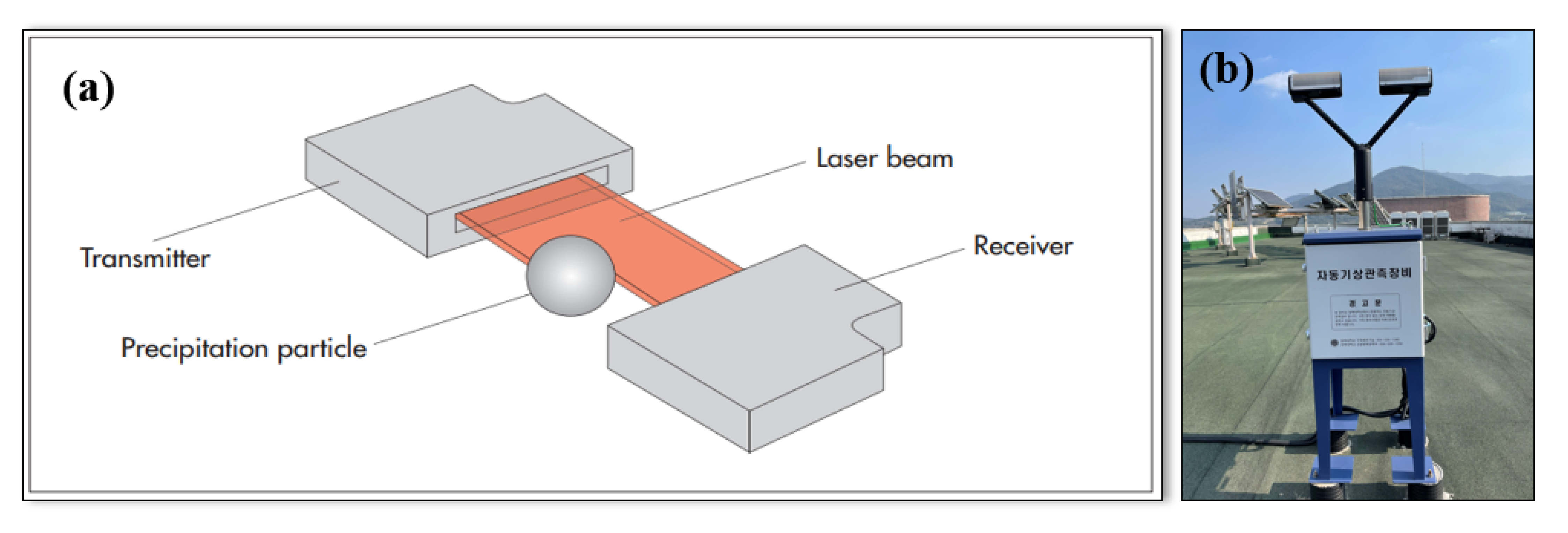
The OTT Parsivel² disdrometer is an optical sensor that creates a 30 mm wide, 180 mm long, and 1 mm high laser beam (Figure 2a). The functional principle is based on the following premise [35]: (a) If no raindrops cross the laser beam, maximum voltage is generated at the receiver. (b) Raindrops obstruct a portion of the laser beam proportional to its diameter as they travel across the beam; the resulting reduction in the output voltage determines the particle size. (c) A signal is created when a raindrop reaches the light strip, and is terminated when the raindrop completely departs the light strip. The duration of the signal determines the velocities of the particles.

After obtaining the volume equivalent diameter (D) and particle speed (V), the disdrometer divides particles into relevant categories, including measurement ranges of 0.2 to 8.0 mm for liquid precipitation particles and 0.2 to 25 mm for solid precipitation particles (i.e., hail and snow). Precipitation particles may move at rates of 0.2 to 20.0 m/s, with a lower scale for small, slow particles than for large, fast particles. The observed particles in a two-dimensional field are classified into 32 V and D classes [35].

Figure 2. (a) Functional principle of the Parsivel² disdrometer (Source: Operating instructions Present Wether Sensor OTT Parsivel² [35]) and (b) the Parsivel² located inside the Kyungpook National University, Sangju campus.

Figure 2. (a) Functional principle of the Parsivel² disdrometer (Source: Operating instructions Present Wether Sensor OTT Parsivel² [35]) and (b) the Parsivel² located inside the Kyungpook National University, Sangju campus.

2.3. Methodology

The schemes outlined below (Figure 3) describe the steps of our work.

• An OTT Parsivel² disdrometer was installed on top of a Kyungpook National University building 80 m above sea level (Figure 2b). Beginning in June 2020, the disdrometer was used to automatically monitor rainfall characteristics at 10-s intervals. This device was then linked to a laptop so that the measured data could be automatically stored.
• Selected precipitation events (Table 1) were categorized based on strict criteria [16,18,19]: (i) two different rainfall events must be separated by at least 6 h, (ii) total rainfall accumulation must exceed 3 mm, and (iii) a storm event length and its average intensity must exceed 30 min and 0.1 mm/h, respectively. The information in Table 1 pertains to specified precipitation events. Subsequently, each event was rigorously examined for outliers in the I_r distribution. Raindrops colliding with the protective covers of the disdrometer and combined with other raindrops may disrupt the laser zone, leading to larger raindrops [16]. During storms, two raindrops may instantaneously travel through the sensor, producing in an inflated, abnormally-high intensity value [19]. Consequently, records with abnormally high-intensity levels were deemed outliers and removed.

Table 1. Information of specified precipitation events.

Event	Date (dd/mm/yy hh:mm)	Duration	No. of Raindrops	No. of Outliers	Rain Depth (mm)		Intensity (mm/h)
						Max	Mean	Median	St. Dev	Skewness
1	10/06/2020 20:51	09 h 30 min	307,808	119	50.46	17.87	4.70	4.00	4.26	0.87
2	13/06/2020 19:54	13 h 42 min	385,208	431	29.75	7.4	1.36	0.21	1.85	1.49
3	24/06/2020 12:45	26 h 31 min	347,936	1573	14.91	1.22	0.20	0.10	0.24	2.37
4	12/03/2021 10:40	06 h 01 min	95,761	93	9.69	3.95	1.44	1.31	0.87	0.65
5	27/03/2021 13:25	14 h 04 min	359,840	117	24.08	5.01	1.61	1.47	1.14	0.60
6	03/04/2021 10:20	21 h 06 min	714,019	314	34.15	5.20	1.35	0.98	1.24	1.02
7	12/04/2021 11:53	13 h 36 min	223,265	202	20.18	4.73	1.30	1.08	1.12	0.92
8	01/05/2021 12:32	17 h 09 min	61,303	1088	4.02	0.5	0.13	0.10	0.08	2.89
9	04/05/2021 16:31	09 h 32 min	182,322	326	9.56	3.07	0.65	0.39	0.69	1.41
10	10/05/2021 07:26	25 h 33 min	188,754	1156	18.36	2.05	0.35	0.10	0.47	1.94
11	16/05/2021 18:15	13 h 23 min	512,393	525	14.46	2.55	0.51	0.24	0.57	1.50
12	20/05/2021 09:37	14 h 49 min	743,031	188	20.28	4.38	1.19	0.96	1.04	0.90
13	28/05/2021 11:49	2 h 39 min	92,003	68	19.92	18.24	5.96	4.75	3.92	1.02
14	30/05/2021 22:25	7 h 04 min	51,022	151	9.90	4.71	0.94	0.10	1.22	1.37
15	03/06/2021 10:01	16 h 13 min	484,004	251	25.25	5.68	1.31	0.90	1.31	1.03
16	10/06/2021 20:06	11 h 45 min	149,679	131	14.6	4.34	1.13	0.83	1.04	0.98
17	22/06/2021 19:45	52 min	17,647	22	8.46	32.48	7.37	3.37	8.29	1.35
18	03/07/2021 13:17	15 h	371,419	305	33.4	7.65	1.66	0.76	1.90	1.28
19	05/07/2021 19:18	9 h 04 min	196,799	75	11.95	4.75	1.23	0.82	1.17	1.05
20	06/07/2021 17:13	24 h 40 min	210,285	1704	12.39	0.37	0.12	0.10	0.05	3.15
21	08/07/2021 01:29	4 h 16 min	149,756	99	32.22	19.50	5.71	4.42	4.71	1.05
22	10/07/2021 19:08	03 h 58 min	52,814	208	16.36	4.93	0.70	0.10	1.13	2.06
23	11/07/2021 19:06	40 min	43,737	36	18.97	53.55	14.22	12.40	11.54	1.28
24	27/07/2021 19:33	01 h 01 min	81,024	7	30.5	92.52	26.08	21.43	23.14	0.82
25	01/08/2021 15:47	07 h 15 min	167,090	318	43.74	10.04	1.90	1.15	2.14	1.45
26	08/08/2021 13:55	01 h 21 min	36,583	78	16.12	30.97	4.29	1.24	7.25	2.32
27	10/08/2021 09:54	01 h 13 min	31,325	30	11.09	36.20	6.31	0.78	9.59	1.52
28	23/08/2021 09:09	27 h 49 min	578,908	659	81.07	8.47	1.99	1.40	1.98	1.16
29	25/08/2021 16:20	07 h 34 min	137,149	339	12.84	2.87	0.47	0.1	0.69	2.00
30	27/08/2021 08:59	8 h 17 min	118,828	138	16.63	8.33	1.55	0.19	2.22	1.41
31	01/09/2021 02:48	13 h 21 min	286,138	404	51.13	11.05	2.09	0.73	2.59	1.34
32	06/09/2021 16:38	21 h 54 min	290,235	837	30.94	3.72	0.65	0.11	0.88	1.66
33	16/09/2021 23:06	13 h 25 min	320,541	173	39.3	11.13	2.45	1.23	2.72	1.11
34	21/09/2021 07:01	4 h 06 min	86,537	38	10.47	9.40	2.32	1.58	2.25	0.94
35	11/10/2021 02:20	40 h 37 min	695,308	561	22.78	2.20	0.50	0.29	0.49	1.15
36	15/10/2021 16:26	14 h 19 min	210,792	419	14.26	2.79	0.75	0.57	0.64	1.19
37	30/11/2021 07:22	16 h 04 min	158,070	406	13.98	3.07	0.62	0.17	0.76	1.43

Table 1. Information of specified precipitation events.

Event	Date (dd/mm/yy hh:mm)	Duration	No. of Raindrops	No. of Outliers	Rain Depth (mm)		Intensity (mm/h)
						Max	Mean	Median	St. Dev	Skewness
1	10/06/2020 20:51	09 h 30 min	307,808	119	50.46	17.87	4.70	4.00	4.26	0.87
2	13/06/2020 19:54	13 h 42 min	385,208	431	29.75	7.4	1.36	0.21	1.85	1.49
3	24/06/2020 12:45	26 h 31 min	347,936	1573	14.91	1.22	0.20	0.10	0.24	2.37
4	12/03/2021 10:40	06 h 01 min	95,761	93	9.69	3.95	1.44	1.31	0.87	0.65
5	27/03/2021 13:25	14 h 04 min	359,840	117	24.08	5.01	1.61	1.47	1.14	0.60
6	03/04/2021 10:20	21 h 06 min	714,019	314	34.15	5.20	1.35	0.98	1.24	1.02
7	12/04/2021 11:53	13 h 36 min	223,265	202	20.18	4.73	1.30	1.08	1.12	0.92
8	01/05/2021 12:32	17 h 09 min	61,303	1088	4.02	0.5	0.13	0.10	0.08	2.89
9	04/05/2021 16:31	09 h 32 min	182,322	326	9.56	3.07	0.65	0.39	0.69	1.41
10	10/05/2021 07:26	25 h 33 min	188,754	1156	18.36	2.05	0.35	0.10	0.47	1.94
11	16/05/2021 18:15	13 h 23 min	512,393	525	14.46	2.55	0.51	0.24	0.57	1.50
12	20/05/2021 09:37	14 h 49 min	743,031	188	20.28	4.38	1.19	0.96	1.04	0.90
13	28/05/2021 11:49	2 h 39 min	92,003	68	19.92	18.24	5.96	4.75	3.92	1.02
14	30/05/2021 22:25	7 h 04 min	51,022	151	9.90	4.71	0.94	0.10	1.22	1.37
15	03/06/2021 10:01	16 h 13 min	484,004	251	25.25	5.68	1.31	0.90	1.31	1.03
16	10/06/2021 20:06	11 h 45 min	149,679	131	14.6	4.34	1.13	0.83	1.04	0.98
17	22/06/2021 19:45	52 min	17,647	22	8.46	32.48	7.37	3.37	8.29	1.35
18	03/07/2021 13:17	15 h	371,419	305	33.4	7.65	1.66	0.76	1.90	1.28
19	05/07/2021 19:18	9 h 04 min	196,799	75	11.95	4.75	1.23	0.82	1.17	1.05
20	06/07/2021 17:13	24 h 40 min	210,285	1704	12.39	0.37	0.12	0.10	0.05	3.15
21	08/07/2021 01:29	4 h 16 min	149,756	99	32.22	19.50	5.71	4.42	4.71	1.05
22	10/07/2021 19:08	03 h 58 min	52,814	208	16.36	4.93	0.70	0.10	1.13	2.06
23	11/07/2021 19:06	40 min	43,737	36	18.97	53.55	14.22	12.40	11.54	1.28
24	27/07/2021 19:33	01 h 01 min	81,024	7	30.5	92.52	26.08	21.43	23.14	0.82
25	01/08/2021 15:47	07 h 15 min	167,090	318	43.74	10.04	1.90	1.15	2.14	1.45
26	08/08/2021 13:55	01 h 21 min	36,583	78	16.12	30.97	4.29	1.24	7.25	2.32
27	10/08/2021 09:54	01 h 13 min	31,325	30	11.09	36.20	6.31	0.78	9.59	1.52
28	23/08/2021 09:09	27 h 49 min	578,908	659	81.07	8.47	1.99	1.40	1.98	1.16
29	25/08/2021 16:20	07 h 34 min	137,149	339	12.84	2.87	0.47	0.1	0.69	2.00
30	27/08/2021 08:59	8 h 17 min	118,828	138	16.63	8.33	1.55	0.19	2.22	1.41
31	01/09/2021 02:48	13 h 21 min	286,138	404	51.13	11.05	2.09	0.73	2.59	1.34
32	06/09/2021 16:38	21 h 54 min	290,235	837	30.94	3.72	0.65	0.11	0.88	1.66
33	16/09/2021 23:06	13 h 25 min	320,541	173	39.3	11.13	2.45	1.23	2.72	1.11
34	21/09/2021 07:01	4 h 06 min	86,537	38	10.47	9.40	2.32	1.58	2.25	0.94
35	11/10/2021 02:20	40 h 37 min	695,308	561	22.78	2.20	0.50	0.29	0.49	1.15
36	15/10/2021 16:26	14 h 19 min	210,792	419	14.26	2.79	0.75	0.57	0.64	1.19
37	30/11/2021 07:22	16 h 04 min	158,070	406	13.98	3.07	0.62	0.17	0.76	1.43

iii.

Linear [36] and power-law [37] relationships were employed to establish a strong connection between KE_exp and I_r, whereas logarithmic [26] and exponential [38] relationships were applied to link KE_con and I_r. In addition, we conducted a study in Sangju City (Korea) to determine the comprehensive relationship between KE and I_r; the results showed that the best fit between KE_exp and I_r was obtained using a power-law form, whereas the closest match between KE_con and I_r was discovered using an exponential equation [17]. Thus, we attempted to gather equations using the power-law and exponential forms for comparison with the data collected in this investigation (Table 2). For various locations, climatic settings, and measurement methods, equations employed in different forms were also used. The selected equations were then compared to the observed KE data from 37 rainfall events with three statistical criteria (See Section v).

Table 2. Information about the 27 KE–I_r equation used in this study. Acronyms: A—tropical climates, B—dry climates, C—temperate climates, AD—acoustic disdrometer, OD—optical disdrometer (P—Parsivel, P²—Parsivel²), FP—flour pellet, and CA—camera. The climate zone is based on Köppen–Geiger climate classification [39].

	Equation	Location	Altitude (m. a.s.l.)	Method	Climate Zone	Source
EXP1	21.1${\mathrm{I}}_{\mathrm{r}}{}^{1.156}$	USA	n.a.	n.a.	A	[40]
EXP2	24.48 (${\mathrm{I}}_{\mathrm{r}}$ − 1.235)	Australia	25	AD	B	[41]
EXP3	28.3${\mathrm{I}}_{\mathrm{r}}$(1 − 0.52${\mathrm{e}}^{-{0.042\mathrm{I}}_{\mathrm{r}}})$	Universal	n.a.	n.a.	n.a.	[38]
EXP4	13${\mathrm{I}}_{\mathrm{r}}{}^{1.21}$	USA	n.a.	CA	A	[42]
EXP5	11${\mathrm{I}}_{\mathrm{r}}{}^{1.25}$	USA	n.a.	AD	A	[43]
EXP6	23.4${\mathrm{I}}_{\mathrm{r}}$ − 18	Spain	n.a.	AD	B	[36]
EXP7	29.02${\mathrm{I}}_{\mathrm{r}}$ − 71.67	Philippines	44	AD	A	[18]
EXP8	12.05${\mathrm{I}}_{\mathrm{r}}{}^{1.19}$	Philippines	44	AD	A	[18]
EXP9	5.9${\mathrm{I}}_{\mathrm{r}}{}^{1.37}$	Cape Verde	321	OD-P	A	[20]
EXP10	30.4${\mathrm{I}}_{\mathrm{r}}$	Cape Verde	321	OD-P	A	[20]
EXP11	23.97${\mathrm{I}}_{\mathrm{r}}$ − 24.28	Korea (Daejeon)	58	O-P	C	[16]
EXP12	12.49${\mathrm{I}}_{\mathrm{r}}{}^{1.16}$	Korea (Daejeon)	58	OD-P	C	[16]
EXP13	7.62${\mathrm{I}}_{\mathrm{r}}{}^{1.3}$	Korea (Sangju)	80	OD-P2	C	[17]
CON1	$29.2 \left(1-0.89\exp \left(-0.048{\mathrm{I}}_{\mathrm{r}}\right)\right)$	Zimbabwe	1230	FP	C	[44]
CON2	$29.3 \left(1-0.28\exp \left(-0.018{\mathrm{I}}_{\mathrm{r}}\right)\right)$	USA (Florida)	3	CA	A	[44]
CON3	$29.0 \left(1-0.59\exp \left(-0.04{\mathrm{I}}_{\mathrm{r}}\right)\right)$	Australia	25	AD	B	[41]
CON4	$29.0 \left(1-0.72\exp \left(-0.05{\mathrm{I}}_{\mathrm{r}}\right)\right)$	USA	180	FP	A	[33]
CON5	$35.9 \left(1-0.56\exp \left(-0.034{\mathrm{I}}_{\mathrm{r}}\right)\right)$	Portugal	21	AD	C	[45]
CON6	$38.4 \left(1-0.54\exp \left(-0.029{\mathrm{I}}_{\mathrm{r}}\right)\right)$	Spain	25	OD	B	[46]
CON7	$36.8 \left(1-0.69\exp \left(-0.038{\mathrm{I}}_{\mathrm{r}}\right)\right)$	Hong Kong	50	AD	C	[47]
CON8	$28.3 \left(1-0.52\exp \left(-0.042{\mathrm{I}}_{\mathrm{r}}\right)\right)$	Universal	n.a.	n.a.	n.a.	[38]
CON9	$30.8 \left(1-0.05\exp \left(-0.03{\mathrm{I}}_{\mathrm{r}}\right)\right)$	Philippines	44	AD-RD80	A	[18]
CON10	$29.8 \left(1-0.60\exp \left(-0.07{\mathrm{I}}_{\mathrm{r}}\right)\right)$	Slovenia (Koseze)	595	OD-P	C	[19]
CON11	$35 \left(1-0.79\exp \left(-0.03{\mathrm{I}}_{\mathrm{r}}\right)\right)$	Cape Verde	321	OD-P	A	[20]
CON12	$25.75 \left(1-0.54\exp \left(-0.05{\mathrm{I}}_{\mathrm{r}}\right)\right)$	Korea (Daejeon)	58	OD-P	C	[16]
CON13	8.163 + 1.949log(Ir)	Korea (Seoul)	42	OD-P	C	[48]
CON14	10.47 + 2.47log(Ir)	Korea (Anseong)	62	OD-P	C	[49]
CON15	30.03 (1 − 0.74exp(−0.068Ir))	Korea (Daegwallyeong)	732	OD-P	C	[50]
CON16	26.5 (1 − 0.94exp(−0.14Ir))	Korea (Sangju)	80	OD-P2	C	[17]

EXP denotes KE_exp types and CON denotes KE_con types. EXP13 and CON16 represent fitted lines of observed data.

Table 2. Information about the 27 KE–I_r equation used in this study. Acronyms: A—tropical climates, B—dry climates, C—temperate climates, AD—acoustic disdrometer, OD—optical disdrometer (P—Parsivel, P²—Parsivel²), FP—flour pellet, and CA—camera. The climate zone is based on Köppen–Geiger climate classification [39].

	Equation	Location	Altitude (m. a.s.l.)	Method	Climate Zone	Source
EXP1	21.1${\mathrm{I}}_{\mathrm{r}}{}^{1.156}$	USA	n.a.	n.a.	A	[40]
EXP2	24.48 (${\mathrm{I}}_{\mathrm{r}}$ − 1.235)	Australia	25	AD	B	[41]
EXP3	28.3${\mathrm{I}}_{\mathrm{r}}$(1 − 0.52${\mathrm{e}}^{-{0.042\mathrm{I}}_{\mathrm{r}}})$	Universal	n.a.	n.a.	n.a.	[38]
EXP4	13${\mathrm{I}}_{\mathrm{r}}{}^{1.21}$	USA	n.a.	CA	A	[42]
EXP5	11${\mathrm{I}}_{\mathrm{r}}{}^{1.25}$	USA	n.a.	AD	A	[43]
EXP6	23.4${\mathrm{I}}_{\mathrm{r}}$ − 18	Spain	n.a.	AD	B	[36]
EXP7	29.02${\mathrm{I}}_{\mathrm{r}}$ − 71.67	Philippines	44	AD	A	[18]
EXP8	12.05${\mathrm{I}}_{\mathrm{r}}{}^{1.19}$	Philippines	44	AD	A	[18]
EXP9	5.9${\mathrm{I}}_{\mathrm{r}}{}^{1.37}$	Cape Verde	321	OD-P	A	[20]
EXP10	30.4${\mathrm{I}}_{\mathrm{r}}$	Cape Verde	321	OD-P	A	[20]
EXP11	23.97${\mathrm{I}}_{\mathrm{r}}$ − 24.28	Korea (Daejeon)	58	O-P	C	[16]
EXP12	12.49${\mathrm{I}}_{\mathrm{r}}{}^{1.16}$	Korea (Daejeon)	58	OD-P	C	[16]
EXP13	7.62${\mathrm{I}}_{\mathrm{r}}{}^{1.3}$	Korea (Sangju)	80	OD-P2	C	[17]
CON1	$29.2 \left(1-0.89\exp \left(-0.048{\mathrm{I}}_{\mathrm{r}}\right)\right)$	Zimbabwe	1230	FP	C	[44]
CON2	$29.3 \left(1-0.28\exp \left(-0.018{\mathrm{I}}_{\mathrm{r}}\right)\right)$	USA (Florida)	3	CA	A	[44]
CON3	$29.0 \left(1-0.59\exp \left(-0.04{\mathrm{I}}_{\mathrm{r}}\right)\right)$	Australia	25	AD	B	[41]
CON4	$29.0 \left(1-0.72\exp \left(-0.05{\mathrm{I}}_{\mathrm{r}}\right)\right)$	USA	180	FP	A	[33]
CON5	$35.9 \left(1-0.56\exp \left(-0.034{\mathrm{I}}_{\mathrm{r}}\right)\right)$	Portugal	21	AD	C	[45]
CON6	$38.4 \left(1-0.54\exp \left(-0.029{\mathrm{I}}_{\mathrm{r}}\right)\right)$	Spain	25	OD	B	[46]
CON7	$36.8 \left(1-0.69\exp \left(-0.038{\mathrm{I}}_{\mathrm{r}}\right)\right)$	Hong Kong	50	AD	C	[47]
CON8	$28.3 \left(1-0.52\exp \left(-0.042{\mathrm{I}}_{\mathrm{r}}\right)\right)$	Universal	n.a.	n.a.	n.a.	[38]
CON9	$30.8 \left(1-0.05\exp \left(-0.03{\mathrm{I}}_{\mathrm{r}}\right)\right)$	Philippines	44	AD-RD80	A	[18]
CON10	$29.8 \left(1-0.60\exp \left(-0.07{\mathrm{I}}_{\mathrm{r}}\right)\right)$	Slovenia (Koseze)	595	OD-P	C	[19]
CON11	$35 \left(1-0.79\exp \left(-0.03{\mathrm{I}}_{\mathrm{r}}\right)\right)$	Cape Verde	321	OD-P	A	[20]
CON12	$25.75 \left(1-0.54\exp \left(-0.05{\mathrm{I}}_{\mathrm{r}}\right)\right)$	Korea (Daejeon)	58	OD-P	C	[16]
CON13	8.163 + 1.949log(Ir)	Korea (Seoul)	42	OD-P	C	[48]
CON14	10.47 + 2.47log(Ir)	Korea (Anseong)	62	OD-P	C	[49]
CON15	30.03 (1 − 0.74exp(−0.068Ir))	Korea (Daegwallyeong)	732	OD-P	C	[50]
CON16	26.5 (1 − 0.94exp(−0.14Ir))	Korea (Sangju)	80	OD-P2	C	[17]

EXP denotes KE_exp types and CON denotes KE_con types. EXP13 and CON16 represent fitted lines of observed data.

iv.

Kinnell suggested an exponential form (Equation (1)) that is mostly used to link KE_con with I_r [44].

KE_con = a (1 − b exp(−c I_r))

(1)

where a, b, and c are empirical parameters.

According to Kinnell, the value of a parameter may be considered to be 29 J m²mm⁻¹ worldwide, and the values of b and c parameters vary and depend on local sites [51]. However, other scientists have provided unique parameter values, demonstrating their high dependency on the geographical setting (Table 2). Based on re-analysis, the empirical parameters in Equation (CON8) for worldwide applications proposed by Van Dijk et al. are the averages derived by fitting the relationship to observed precipitation KE data taken from different locations, including Panama, Indonesia, the United States, the Marshall Islands, Australia, and Portugal [38]. Thus, we propose a Korean equation (Equation (2)) based on the approach of Van Dijk et al. [38].

KE_con = 27.4(1 − 0.74exp(−0.086I_r))

(2)

where 27.4, 0.74, and 0.086 are the averages derived from the KE_con–I_r relationship in three Korean locations (Figure 1): Daejeon (CON12), Daegwallyeong (CON15), and Sangju (CON16).

v.

Several statistical measures were used to assess the recorded and predicted KE values estimated using the 27 KE–I_r equations.

Table 3. Description of the evaluation criteria used in this research (a_i: observations; b_i: forecasts; $\overline{\mathrm{a}}$: mean of recorded values, $\overline{\mathrm{b}}:$ mean of forecasted values, n: number of samples).

Name	Equation	Available Range	Best Value
RMSE	$\sqrt{\frac{1}{\mathrm{n}}{{\displaystyle \sum }}_{\mathrm{i}=1}^{\mathrm{n}}{\left({\mathrm{a}}_{\mathrm{i}}-{\mathrm{b}}_{\mathrm{i}}\right)}^2}$	0.0 to +∞	0.0
MAE	$\frac{1}{\mathrm{n}}{{\displaystyle \sum }}_{\mathrm{i}=1}^{\mathrm{n}}\left|{\mathrm{a}}_{\mathrm{i}}{–\mathrm{b}}_{\mathrm{i}}\right|$	0.0 to +∞	0.0
R2	$\frac{{\left[{{\displaystyle \sum }}_{\mathrm{i}=1}^{\mathrm{n}}\left({\mathrm{a}}_{\mathrm{i} }– \overline{\mathrm{a}}\right)\left({\mathrm{b}}_{\mathrm{i}} – \overline{\mathrm{b}}\right)\right]}^2}{{{\displaystyle \sum }}_{\mathrm{i}=1}^{\mathrm{n}}{\left({\mathrm{a}}_{\mathrm{i}}– \overline{\mathrm{a}}\right)}^2{{\displaystyle \sum }}_{\mathrm{i}=1}^{\mathrm{n}}{\left({\mathrm{b}}_{\mathrm{i}} – \overline{\mathrm{b}}\right)}^2}$	0.0 to 1.0	1.0

presents the specifics of the evaluation criteria, and the validity of empirical equations was visually evaluated using goodness-of-fit plots.

3. Results

3.1. KE–I_r Relationships: Comparison

3.1.1. Kinetic Energy Expenditure

Rainfall KE and I_r are constrained by the microphysics of the in situ climate and meteorological factors. Thus, it is critical to benchmark several equations worldwide to determine their efficiency and accuracy in Korea.

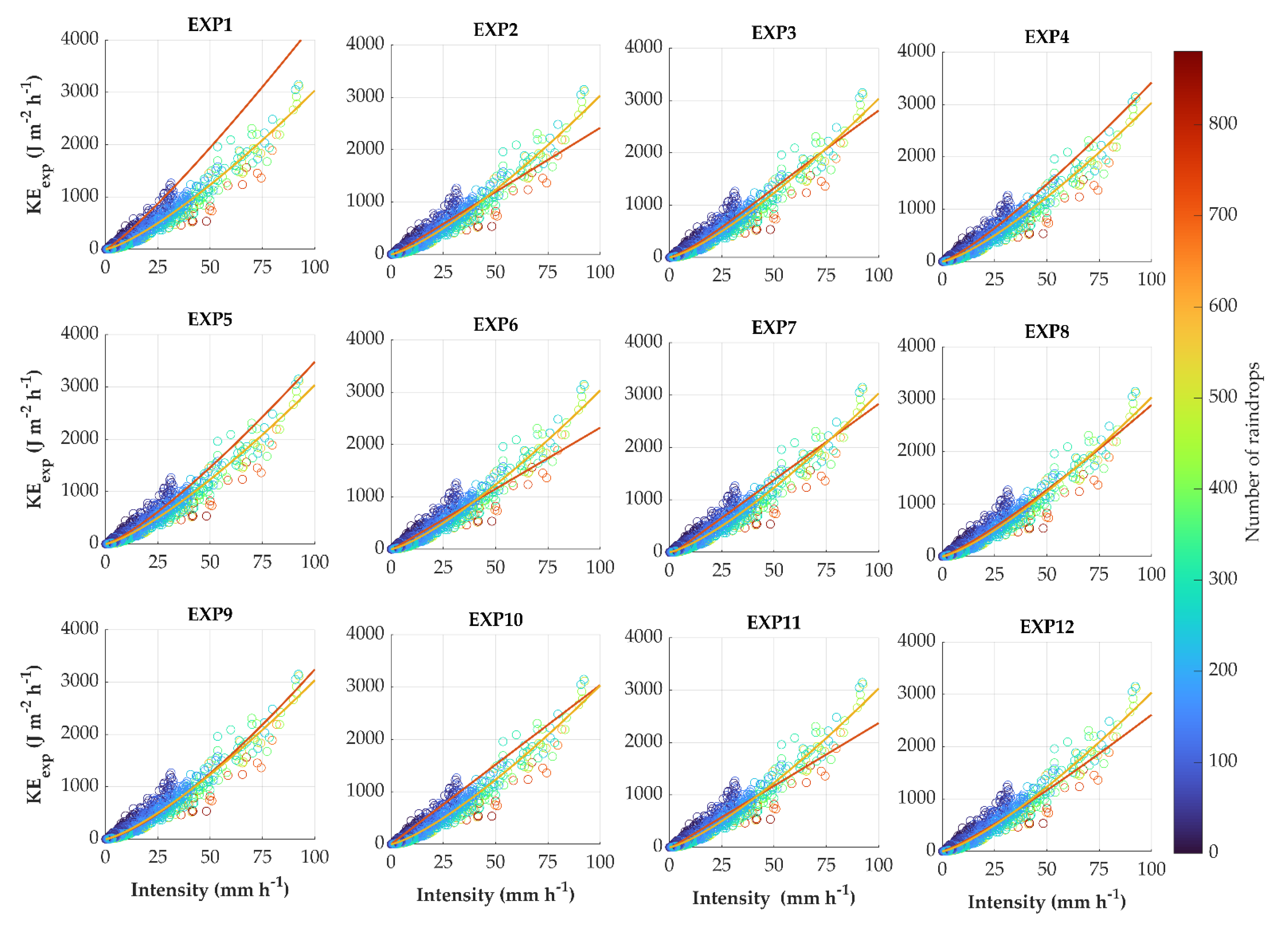
First, we examined the performance of the 12 KE_exp–I_r equations calibrated at various global locations. Each of the KE estimations produced by the 12 equations was compared with the actual KE data taken at our monitoring site. The performances of the 12 equations are shown in Figure 4. Table 4 and Figure 5 provide information about comparable findings of the 12 equations, all of which predicted good results of KE_exp values, except for EXP1 (R² = 0.37), EXP7 (R² = 0.46), and EXP10 (R² = 0.43). The rest of the equations produced accurate results, with R² ranging from 0.72 (EXP2) to 0.94 (EXP9). The performance of EXP9 appears good, even though that site (Cape Verde Islands) has a very different environment from Korea. It is also noticeable that half of the 12 benchmarked equations have a power-law structure and provide accurate predictions of KE_exp values (except for EXP1). The performance of EXP7 and EXP8 show a total difference, even though they were conducted in the same region and climate pattern (Philippines). This indicates that the power form (EXP8) outperformed the linear form (EXP7) in this test. The EXP9 is the most suitable equation for predicting KE_exp values, with the highest R² (0.94) and lowest RMSE and MAE (i.e., 14.08 J m⁻²h⁻¹ and 3.85 J m⁻²h⁻¹, respectively), followed by EXP8 (R² = 0.92, RMSE = 16.24 J m⁻²h⁻¹, and MAE = 6.72 J m⁻²h⁻¹).

The power-law form of EXP12, conducted in the Korean area, was also in line with the observed data (R² = 0.92, RMSE = 16.23 J m⁻²h⁻¹, and MAE = 6.79 J m⁻²h⁻¹). This could be accounted for by the fact that the location where the equation was developed and the location where our data were collected both had similar rainfall patterns.

Figure 4. Comparison of 12 KE_exp equations (represented by red lines) with measured data. The yellow line represents the fitted line of measured data (EXP13).

Figure 4. Comparison of 12 KE_exp equations (represented by red lines) with measured data. The yellow line represents the fitted line of measured data (EXP13).

Figure 5. Statistical analysis results of 12 KE_exp–I_r relationships with observed data.

Figure 5. Statistical analysis results of 12 KE_exp–I_r relationships with observed data.

Table 4. Statistical analysis results of 12 relationships between KE_exp and I_r in the literature.

Equation	R2	RMSE (J m−2h−1)	MAE (J m−2h−1)
EXP1	0.37	45.57	19.08
EXP2	0.75	27.90	22.47
EXP3	0.91	17.01	7.83
EXP4	0.86	21.26	8.40
EXP5	0.89	18.83	6.53
EXP6	0.83	23.39	15.73
EXP7	0.46	58.61	54.22
EXP8	0.92	16.24	6.72
EXP9	0.94	14.08	3.85
EXP10	0.43	43.56	24.98
EXP11	0.81	25.20	18.88
EXP12	0.92	16.23	6.79

Table 4. Statistical analysis results of 12 relationships between KE_exp and I_r in the literature.

Equation	R2	RMSE (J m−2h−1)	MAE (J m−2h−1)
EXP1	0.37	45.57	19.08
EXP2	0.75	27.90	22.47
EXP3	0.91	17.01	7.83
EXP4	0.86	21.26	8.40
EXP5	0.89	18.83	6.53
EXP6	0.83	23.39	15.73
EXP7	0.46	58.61	54.22
EXP8	0.92	16.24	6.72
EXP9	0.94	14.08	3.85
EXP10	0.43	43.56	24.98
EXP11	0.81	25.20	18.88
EXP12	0.92	16.23	6.79

3.1.2. Kinetic Energy Content

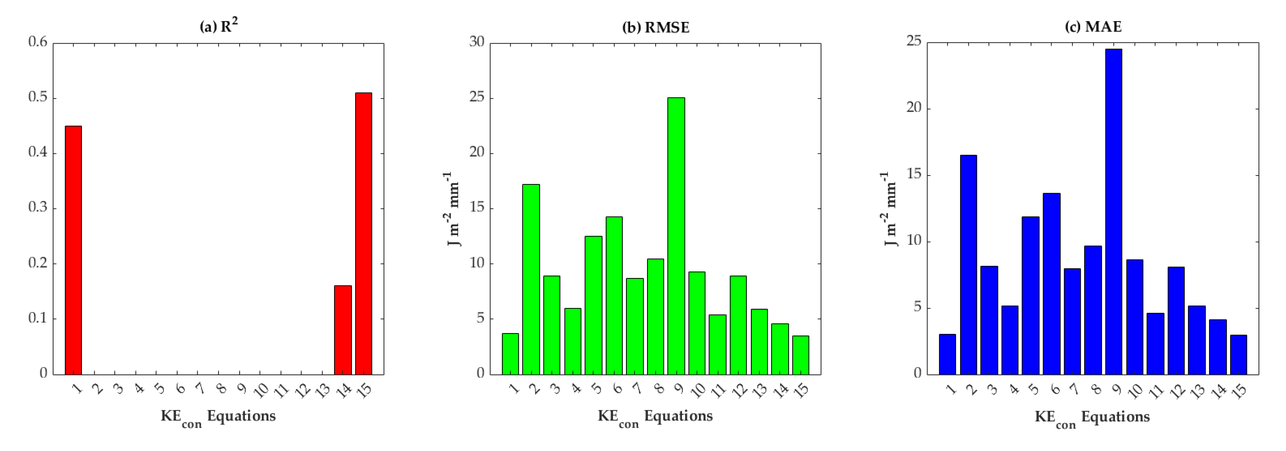
To further assess the influence of local climate, geography, and precipitation, we tested the performance of the 15 KE_con–I_r equations. It is noted that the KE_con–I_r equations performed poorly compared with KE_exp–I_r equations (Figure 5 and Figure 6). Figure 7 illustrates a side-by-side comparison of the performance of these equations. The main reason for the cause of the low R² values in Table 5 comes from the formation of KE_exp and KE_con–I_r relationships, since the R² from the formation of KE_exp–I_r equations is always higher than that of KE_con–I_r [16,17,18,19,20]. It is noted that the observation of KE_exp tends to follow a narrow and predictable trend, whereas the tendency of KE_con values is entirely different and scattered, making the development of accurate mathematical expressions more challenging to forecast.

According to the statistical data in Table 5 and Figure 6, all 13 equations produced very low R², except for CON1 (0.45) and CON15 (0.51). The latter performed the best at our research site because it had the lowest RMSE (3.49 J m⁻²mm⁻¹) and MAE (2.96 J m⁻²mm⁻¹). While CON1 and CON15 are considered mountainous sites (1230 m a.s.l. and 732 m a.s.l., respectively) compared to our study area (80 m a.s.l.), it is assumed that the relationships would be different due to the effect of altitude [52]. The performance of CON1 was good (R² = 0.45, RMSE = 3.71 J m⁻²mm⁻¹, MAE = 3.05 J m⁻²mm⁻¹), and this can be explained by the fact that both locations (CON1 and CON16) experienced the same predominantly temperate climates.

CON9 showed the poorest performance (RMSE = 25.03 J m⁻²mm⁻¹, MAE = 24.54 J m⁻²mm⁻¹) in this benchmark due to the difference in climate zone and the measurement method involved. Based on a re-analysis of several KE_con–I_r connections discovered globally, Van Dijk et al. suggested a global KE_con–I_r equation (CON8) [39]. However, it seems as if the equation is ineffective and inapplicable in Korea based on the statistical evidence from Table 5 (R² = 0.00, RMSE = 10.43 J m⁻²mm⁻¹, MAE = 9.67 J m⁻²mm⁻¹).

The statistical results in Table 5 showed the uncertainty and inconsistency between the performance of four equations established in Korea (CON12–15). It is worth noting that the structures of CON13 and CON14 are logarithmic. Estimation of KE_con based on logarithmic forms indicates that KE_con has no upper bound, but other research has shown the contrary; that the exponential equation reaches a maximum KE_con value and then stays stable independent of I_r [41,44]. Since KE_con has a maximum value (specified as the parameter a in Equation (1)), the exponential equation is preferable to the others for estimating KE_con values. The maximum of KE_con value of CON15 (30.03 J m⁻²mm⁻¹) is significantly higher than that of CON12 (25.75 J m⁻²mm⁻¹) and CON16 (26.5 J m⁻²mm⁻¹), and the location of the equation can explain this. CON15 is considered a mountainous site (732 m a.s.l.) compared to the lower altitude areas of CON 12 and CON16 (58 m a.s.l. and 80 m a.s.l., respectively). This phenomenon was consistent with a study by Petan et al. when they observed that KE values were higher at higher elevations for the same rainfall patterns in Slovenia [19]. Furthermore, high wind from the coastal site of CON15 (Figure 1) that causes non-vertical raindrop movements may also distort drop size distribution (DSD) predictions, leading to the difference in KE estimations. The further disparities in the result outputs will be discussed in Section 4.

Figure 6. Statistical analysis results of 15 KE_con–I_r relationships with observed data.

Figure 6. Statistical analysis results of 15 KE_con–I_r relationships with observed data.

Table 5. Statistical analysis of 15 KE_con–I_r equations in the literature.

Equation	R2	$\mathbf{RMSE} (\mathbf{J} {\mathbf{m}}^{-2}{\mathbf{mm}}^{-1})$	$\mathbf{MAE} (\mathbf{J} {\mathbf{m}}^{-2}{\mathbf{mm}}^{-1})$
CON1	0.45	3.71	3.05
CON2	-	17.18	16.53
CON3	-	8.94	8.17
CON4	-	5.95	5.21
CON5	-	12.53	11.89
CON6	-	14.25	13.64
CON7	-	8.68	7.97
CON8	-	10.43	9.67
CON9	-	25.03	24.54
CON10	-	9.29	8.65
CON11	-	5.36	4.63
CON12	-	8.90	8.12
CON13	- 1	5.88	5.21
CON14	0.16	4.59	4.13
CON15	0.51	3.49	2.96

¹ denotes minimal values of R².

Table 5. Statistical analysis of 15 KE_con–I_r equations in the literature.

Equation	R2	$\mathbf{RMSE} (\mathbf{J} {\mathbf{m}}^{-2}{\mathbf{mm}}^{-1})$	$\mathbf{MAE} (\mathbf{J} {\mathbf{m}}^{-2}{\mathbf{mm}}^{-1})$
CON1	0.45	3.71	3.05
CON2	-	17.18	16.53
CON3	-	8.94	8.17
CON4	-	5.95	5.21
CON5	-	12.53	11.89
CON6	-	14.25	13.64
CON7	-	8.68	7.97
CON8	-	10.43	9.67
CON9	-	25.03	24.54
CON10	-	9.29	8.65
CON11	-	5.36	4.63
CON12	-	8.90	8.12
CON13	- 1	5.88	5.21
CON14	0.16	4.59	4.13
CON15	0.51	3.49	2.96

¹ denotes minimal values of R².

Figure 7. Comparison of 15 KE_con equations (represented by red lines) with measured data. The yellow line represents the fitted line of measured data (CON16).

Figure 7. Comparison of 15 KE_con equations (represented by red lines) with measured data. The yellow line represents the fitted line of measured data (CON16).

3.2. KE–I_r Relationships: Proposition

The previous section illustrated the variances in meteorological settings owing to complex orography and other geographical factors, as well as disparities in instrumental sensitivity, which can potentially contribute to the differences in these empirical parameters in Table 2. Consequently, we meticulously selected the most suitable equations (iv in Section 2.3) that satisfy the same requirements in measurement methodology, mathematical functions, climatic conditions, and statistical performance with observed data.

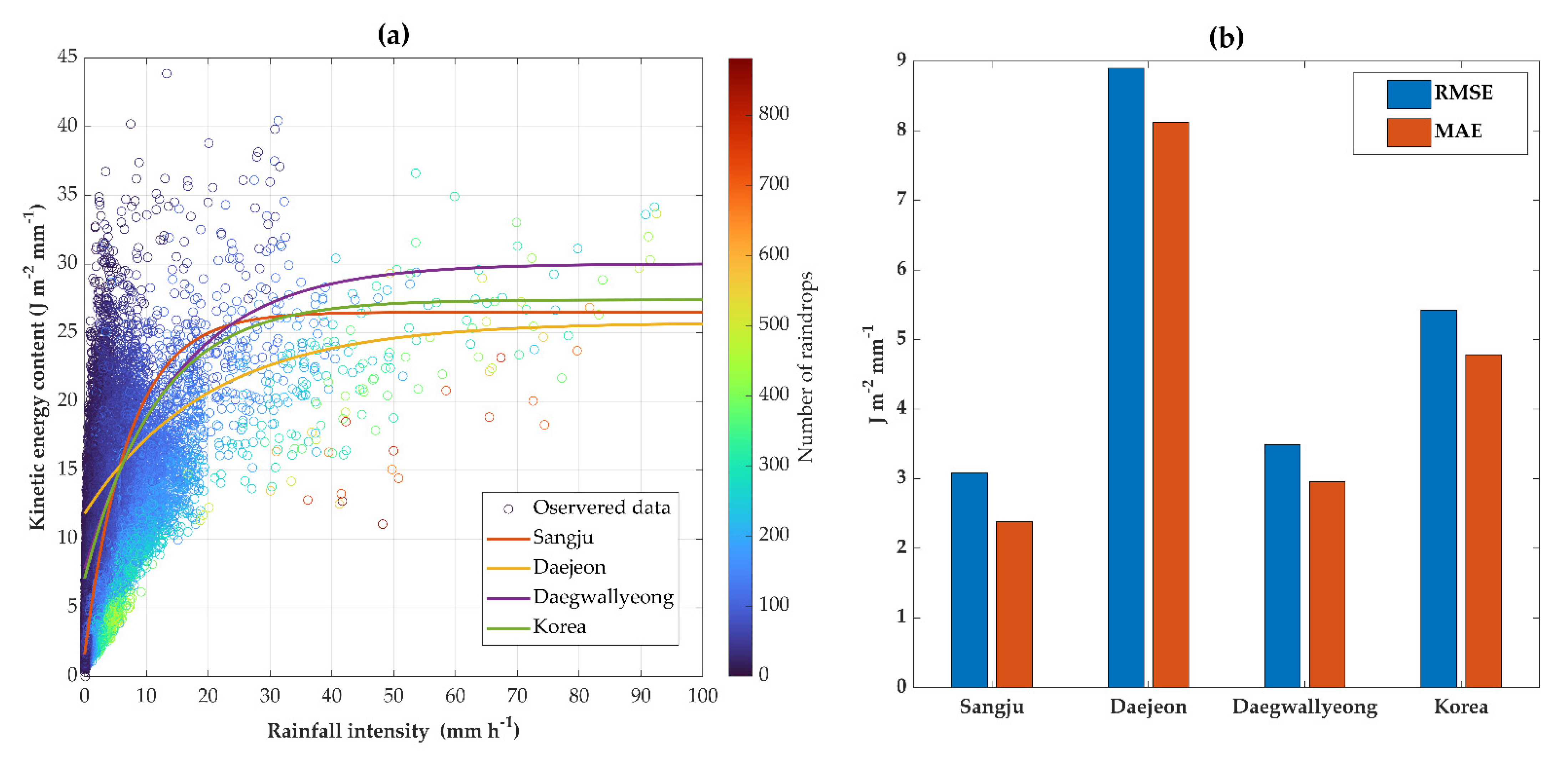
The proposed KE_con–I_r equation for the Korean area (Equation (2)) was drawn and compared with the observed KE_con data in Figure 8a, and the goodness-of-fit statistics are shown in Figure 8b. It is noted that the Korean equation yielded a good performance, with the RMSE and MAE values being 5.42 and 4.78 J m⁻²mm⁻¹, respectively. However, this equation overestimates KE_con values in low-intensity zones, particularly when I_r is zero. Compared to the performance of the Daejeon equation, the performance of the Korean equation is more robust, but it is worse than the performance of the Sangju and Daegwallyeong equations.

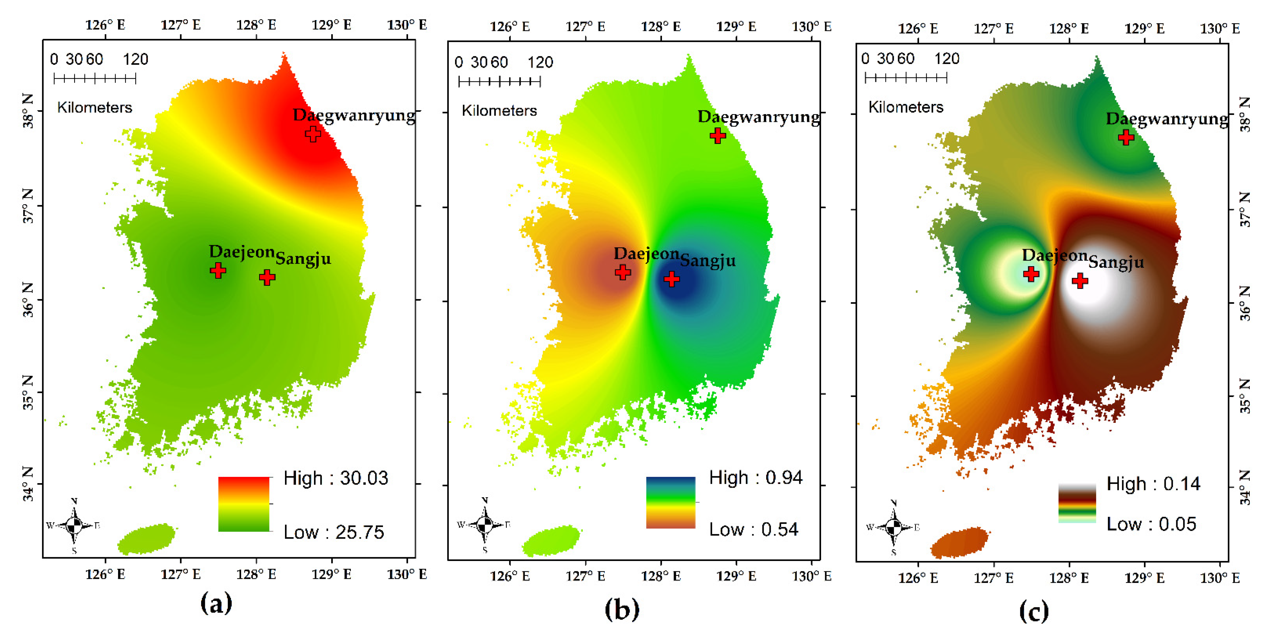
The spatial distribution of a, b, and c parameters in Equation (2) showed a high variance in geography (Figure 9). The value of a parameter (Figure 9a), which denotes the maximum KE_con, is the highest (30.03 J m⁻²mm⁻¹) in the northern part of Korea. These findings are in agreement with earlier research by Salles et al. that the b and c parameters are site-specific (Figure 9b,c) [53]. Reported values for a parameters in Table 2 range from 27.75 to 38.4 m⁻²mm⁻¹, 0.05–0.89 for b parameters, and 0.018–0.07 for c parameters.

4. Discussion

Several factors could be attributed to the disparities in parameter values across numerous studies (Table 2) and disparities in the result outputs. These might be categorized as discrepancies in measurement methodologies, geographical sites, and meteorological patterns.

4.1. Measurement Method

To measure drop size distributions or KE, the authors have used various techniques (Table 2), and each has its own limitations and potential sources of error, which certainly contributed to some of the differences across research.

Sarkar et al. evaluated the comprehensive performance of three raindrop size methods in India, including the Joss–Waldvogel disdrometer [54]. The results indicated that the disdrometer had a low sensitivity for detecting extremely tiny drops (<0.5 mm) and failed to capture drops bigger than 5.5 mm. Consequently, the device is dependable for detecting rainfall intensity that is neither too low (<0.1 mm/h) nor too high (>20 mm/h). However, wind may have a significant effect on disdrometer measurements [41]. Beczek et al. used high-speed cameras to calculate the distribution of particle diameters and masses and confirmed that this approach overstated the diameter values [55]. Hall noted that the splashing of big drops may result in the formation of small droplets, which might impair the filter paper approach [56]. According to Niu et al., instrumental error caused tiny raindrops (approximately 0.3 mm in diameter) to have their velocity overestimated, but this problem dropped significantly as drop size increased [57].

A study conducted by Johannsen et al. explored the influence of three disdrometer types (OTT Parsivel, PWS100, and Thies) on the formation of KE–I_r equations [58]. Their findings demonstrated that errors resulting from instrumental variations were related to rainfall characteristics observations by various types of disdrometers. As a result, the detected parameters of the exponential KE_con–I_r equations varied mathematically by disdrometer type. Furthermore, Angulo-Martnez and Barros also noted that the disdrometer sensor also affects the formation of KE–I_r equations since the DSD from disdrometers is inconsistent and might result in several KE–I_r relationships for the same site [59].

4.2. Geographical Features and Meteorological Settings

Given the sampling error-related methods discussed in the preceding sections, geographical features, meteorological patterns, and different types of precipitation may also be responsible for the variance in the KE estimations.

Angulo-Martínez and Barros noted that rainfall DSDs vary greatly across ridges and valleys, as well as between exposed upwind ridges and the inner area for similar rainfall patterns when they evaluated the performance of two Parsivel disdrometers in three regions in the Southern Appalachian Mountains of the U.S. [59]. The findings also revealed a 40% disparity in KE estimations from the same disdrometers.

Tang et al. investigated the behavior of raindrop size distributions in three different areas of mainland China (i.e., Beijing, Yangjiang, and Zhangbei) using Parsivel disdrometers [60]. The authors noted that Zhangbei had the greatest number of raindrops smaller than 1 mm, owning to its greater altitude and evaporation. According to Montero-Martínez et al., altitude may also affect the distribution of raindrop size and velocity, thereby affecting the overall findings of each equation [52]. McIsaac noted that a decrease in KE was predicted at higher altitudes [61]. However, the greater the elevation of a place, the higher the rate of KE values, although scientists were stumped as to why this disparity existed [19].

A study by Johannsen et al. showed that it was unfeasible to provide a single KE–I equation applicable to Austria, the Czech Republic, and New Zealand [58].

5. Conclusions

Research on the spatial and temporal variability of precipitation features is crucial, considering the growing frequency of severe rainfall events globally. Therefore, understanding the link between rainfall intensity (I_r) and kinetic energy (KE) and its temporal and spatial variability is crucial for any physics-based soil erosion model application because KE plays a vital role as an erosivity parameter.

Direct estimation of rainfall KE is not practical and is often confined to space-restricted research. Consequently, most researchers use either theoretical or empirical relationships to establish empirical links between I_r and KE based on data availability. In this study, we compared and evaluated rainfall KE estimations from 27 KE–I_r equations with 37 rainfall events collected using an OTT Parsivel² disdrometer. Based on a re-analysis, we proposed an exponential KE_con–I_r equation for the entire Korean site and illustrated the spatial distribution of their parameters on a map. The findings of this study are listed below.

• Local climate, terrain, and precipitation patterns may affect KE estimates. Significant discrepancies were found when KE values were computed by the disdrometer and compared with 27 equations from different parts of the globe. The statistically most accurate estimates of KE expenditure and KE content in Sangju City were obtained using the power-law equation (R² = 0.94; RMSE = 14.08 J m⁻²h⁻¹, and MAE = J m⁻²h⁻¹) given by Sanchez-Moreno et al. [20] and the exponential equation (R² = 0.51, RMSE = 3.49 J m⁻²mm⁻¹, and MAE = 2.96 J m⁻²mm⁻¹) published by Lee and Won [50], respectively.
  None of these empirical formulations can be employed globally, and their applicability far from the geographical and climatic circumstances under which they are calibrated is restricted. Only places in the dataset or regions with comparable geographic and climatic features might use empirical KE–I_r equations.
• The suggested equation applied to the Korean site (Equation (2)) exhibits a comparable general correlation with the observed KE_con data (RMSE = 5.42 J m⁻²mm⁻¹ and MAE= 4.78 J m⁻²mm⁻¹). However, the equation must be confirmed and benchmarked at different locations in Korea with observed data. Nowadays, optical disdrometers are more affordable, pre-calibrated, and prepared for field use, making them easier to use and facilitate. More precision has been acquired over a large geographical region as more research has been conducted and more equations have been published. However, the same type of optical measuring equipment should be used to properly determine spatial variations in rainfall properties.
  Because of the high variance in the spatial distribution of exponential parameters, any regional application for using KE_con as an erosivity parameter in surface erosion models should be strictly selected based on geographical settings, particularly in areas with complicated terrain where the spatial variability of rainfall is high.

References

1. Zhang, X.; Zhao, W.; Wang, L.; Liu, Y.; Liu, Y.; Feng, Q. Relationship between Soil Water Content and Soil Particle Size on Typical Slopes of the Loess Plateau during a Drought Year. Sci. Total Environ. 2019, 648, 943–954. [Google Scholar] [CrossRef] [PubMed] [Green Version]
2. Archer, N.A.L.; Bonell, M.; Coles, N.; MacDonald, A.M.; Auton, C.A.; Stevenson, R. Soil Characteristics and Landcover Relationships on Soil Hydraulic Conductivity at a Hillslope Scale: A View towards Local Flood Management. J. Hydrol. 2013, 497, 208–222. [Google Scholar] [CrossRef] [Green Version]
3. Boisramé, G.; Thompson, S.; Stephens, S. Hydrologic Responses to Restored Wildfire Regimes Revealed by Soil Moisture–Vegetation Relationships. Adv. Water Resour. 2018, 112, 124–146. [Google Scholar] [CrossRef]
4. Tabari, H. Climate Change Impact on Flood and Extreme Precipitation Increases with Water Availability. Sci. Rep. 2020, 10, 13768. [Google Scholar] [CrossRef] [PubMed]
5. Sun, L.; Zhou, J.L.; Cai, Q.; Liu, S.; Xiao, J. Comparing Surface Erosion Processes in Four Soils from the Loess Plateau under Extreme Rainfall Events. Int. Soil Water Conserv. Res. 2021, 9, 520–531. [Google Scholar] [CrossRef]
6. Wuepper, D.; Borrelli, P.; Finger, R. Countries and the Global Rate of Soil Erosion. Nat. Sustain. 2020, 3, 51–55. [Google Scholar] [CrossRef]
7. Cuomo, S.; Chareyre, B.; d’Arista, P.; Sala, M.D.; Cascini, L. Micromechanical Modelling of Rainsplash Erosion in Unsaturated Soils by Discrete Element Method. Catena 2016, 147, 146–152. [Google Scholar] [CrossRef]
8. Van, L.N.; Le, X.-H.; Nguyen, G.V.; Yeon, M.; Jung, S.; Lee, G. Investigating Behavior of Six Methods for Sediment Transport Capacity Estimation of Spatial-Temporal Soil Erosion. Water 2021, 13, 3054. [Google Scholar] [CrossRef]
9. Lu, J.-Y.; Su, C.-C.; Lu, T.-F.; Maa, M.-M. Number and Volume Raindrop Size Distributions in Taiwan. Hydrol. Process. 2008, 22, 2148–2158. [Google Scholar] [CrossRef]
10. Zhao, L.; Fang, Q.; Hou, R.; Wu, F. Effect of Rainfall Intensity and Duration on Soil Erosion on Slopes with Different Microrelief Patterns. Geoderma 2021, 396, 115085. [Google Scholar] [CrossRef]
11. Torres, D.S.; Salle, S.C.; Creutin, J.D.; Delrieu, G. Quantification of Soil Detachment by Raindrop Impact: Performance of Classical Formulae of Kinetic Energy in Mediterranean Storms. In Proceedings of the Oslo Symposium, Erosion and Sediment Transport Monitoring Programmes in River Basins, Oslo, Norway, 24–28 August 1992; p. 10. [Google Scholar]
12. Madden, L.V.; Wilson, L.L.; Ntahimpera, N. Calibration and Evaluation of an Electronic Sensor for Rainfall Kinetic Energy. Phytopathology 1998, 88, 950–959. [Google Scholar] [CrossRef] [PubMed] [Green Version]
13. Kathiravelu, G.; Lucke, T.; Nichols, P. Rain Drop Measurement Techniques: A Review. Water 2016, 8, 29. [Google Scholar] [CrossRef] [Green Version]
14. Schönhuber, M.; Lammer, G.; Randeu, W.L. The 2D-Video-Distrometer. In Precipitation: Advances in Measurement, Estimation and Prediction; Michaelides, S., Ed.; Springer: Berlin/Heidelberg, Germany, 2008; pp. 3–31. ISBN 978-3-540-77655-0. [Google Scholar]
15. Angulo-Martínez, M.; Beguería, S.; Kyselý, J. Use of Disdrometer Data to Evaluate the Relationship of Rainfall Kinetic Energy and Intensity (KE-I). Sci. Total Environ. 2016, 568, 83–94. [Google Scholar] [CrossRef] [PubMed] [Green Version]
16. Lim, Y.S.; Kim, J.K.; Kim, J.W.; Park, B.I.; Kim, M.S. Analysis of the Relationship between the Kinetic Energy and Intensity of Rainfall in Daejeon, Korea. Quat. Int. 2015, 384, 107–117. [Google Scholar] [CrossRef]
17. Van, L.N.; Le, X.-H.; Nguyen, G.V.; Yeon, M.; May, D.T.T.; Lee, G. Comprehensive Relationships between Kinetic Energy and Rainfall Intensity Based on Precipitation Measurements from an OTT Parsivel2 Optical Disdrometer. Front. Environ. Sci. 2022, 10, 985516. [Google Scholar] [CrossRef]
18. Fornis, R.L.; Vermeulen, H.R.; Nieuwenhuis, J.D. Kinetic Energy–Rainfall Intensity Relationship for Central Cebu, Philippines for Soil Erosion Studies. J. Hydrol. 2005, 300, 20–32. [Google Scholar] [CrossRef]
19. Petan, S.; Rusjan, S.; Vidmar, A.; Mikoš, M. The Rainfall Kinetic Energy–Intensity Relationship for Rainfall Erosivity Estimation in the Mediterranean Part of Slovenia. J. Hydrol. 2010, 391, 314–321. [Google Scholar] [CrossRef]
20. Sanchez-Moreno, J.F.; Mannaerts, C.M.; Jetten, V.; Löffler-Mang, M. Rainfall Kinetic Energy–Intensity and Rainfall Momentum–Intensity Relationships for Cape Verde. J. Hydrol. 2012, 454–455, 131–140. [Google Scholar] [CrossRef]
21. Rose, C.W. Soil detachment caused by rainfall. Soil Sci. 1960, 89, 28–35. [Google Scholar] [CrossRef]
22. Paringit, E.C.; Nadaoka, K. Sediment Yield Modelling for Small Agricultural Catchments: Land-Cover Parameterization Based on Remote Sensing Data Analysis. Hydrol. Process. 2003, 17, 1845–1866. [Google Scholar] [CrossRef]
23. Al-Durrah, M.M.; Bradford, J.M. Parameters for Describing Soil Detachment Due to Single Waterdrop Impact. Soil Sci. Soc. Am. J. 1982, 46, 836–840. [Google Scholar] [CrossRef]
24. Van Dijk, A.I.J.M.; Meesters, A.G.C.A.; Bruijnzeel, L.A. Exponential Distribution Theory and the Interpretation of Splash Detachment and Transport Experiments. Soil Sci. Soc. Am. J. 2002, 66, 1466–1474. [Google Scholar] [CrossRef]
25. Morgan, R.P.C. Soil Erosion and Conservation, 3rd ed.; Blackwell Pub: Malden, MA, USA, 2005; ISBN 978-1-4051-1781-4. [Google Scholar]
26. Wischmeier, W.H.; Smith, D.D. Rainfall Energy and Its Relationship to Soil Loss. Trans. Am. Geophys. Union 1958, 39, 285. [Google Scholar] [CrossRef]
27. Elwell, H.A. Modelling Soil Losses in Southern Africa. J. Agric. Eng. Res. 1978, 23, 117–127. [Google Scholar] [CrossRef]
28. Verstraeten, G.; Oost, K.; Rompaey, A.; Poesen, J.; Govers, G. Evaluating an Integrated Approach to Catchment Management to Reduce Soil Loss and Sediment Pollution through Modelling. Soil Use Manag. 2002, 18, 386–394. [Google Scholar] [CrossRef]
29. Lee, G.; Yu, W.; Jung, K. APIP Catchment-Scale Soil Erosion and Sediment Yield Simulation Using a Spatially Distributed Erosion Model. Environ. Earth Sci. 2013, 70, 33–47. [Google Scholar] [CrossRef]
30. Lin, G.-W.; Chen, H. The Relationship of Rainfall Energy with Landslides and Sediment Delivery. Eng. Geol. 2012, 125, 108–118. [Google Scholar] [CrossRef]
31. Chang, J.-M.; Chen, H.; Jou, B.J.-D.; Tsou, N.-C.; Lin, G.-W. Characteristics of Rainfall Intensity, Duration, and Kinetic Energy for Landslide Triggering in Taiwan. Eng. Geol. 2017, 231, 81–87. [Google Scholar] [CrossRef]
32. Davison, P.; Hutchins, M.G.; Anthony, S.G.; Betson, M.; Johnson, C.; Lord, E.I. The Relationship between Potentially Erosive Storm Energy and Daily Rainfall Quantity in England and Wales. Sci. Total Environ. 2005, 344, 15–25. [Google Scholar] [CrossRef]
33. Brown, L.C.; Foster, G.R. Storm Erosivity Using Idealized Intensity Distributions. Trans. Am. Soc. Agric. Biol. Eng. 1987, 30, 379–386. [Google Scholar] [CrossRef]
34. Serio, M.A.; Carollo, F.G.; Ferro, V. A Method for Evaluating Rainfall Kinetic Power by a Characteristic Drop Diameter. J. Hydrol. 2019, 577, 123996. [Google Scholar] [CrossRef]
35. Operating Instructions Present Weather Sensor OTT Parsivel2. Available online: https://www.ott.com/fr-fr/produits/la-meteorologie-66/ott-parsivel2-174 (accessed on 1 November 2022).
36. Usón, A.; Ramos, M.C. An Improved Rainfall Erosivity Index Obtained from Experimental Interrill Soil Losses in Soils with a Mediterranean Climate. Catena 2001, 43, 293–305. [Google Scholar] [CrossRef]
37. Brodie, I.; Rosewell, C. Theoretical Relationships between Rainfall Intensity and Kinetic Energy Variants Associated with Stormwater Particle Washoff. J. Hydrol. 2007, 340, 40–47. [Google Scholar] [CrossRef]
38. Van Dijk, A.I.J.M.; Bruijnzeel, L.A.; Rosewell, C.J. Rainfall Intensity–Kinetic Energy Relationships: A Critical Literature Appraisal. J. Hydrol. 2002, 261, 1–23. [Google Scholar] [CrossRef]
39. Beck, H.E.; Zimmermann, N.E.; McVicar, T.R.; Vergopolan, N.; Berg, A.; Wood, E.F. Present and Future Köppen-Geiger Climate Classification Maps at 1-Km Resolution. Sci. Data 2018, 5, 180214. [Google Scholar] [CrossRef] [PubMed] [Green Version]
40. Park, S.W.; Mitcell, J.K.; Bubenzer, G.D. An Analysis of Splash Erosion Mechanics; American Society of Agricultural Engineers: St. Joseph, MI, USA, 1980. [Google Scholar]
41. Rosewell, C.J. Rainfall Kinetic Energy in Eastern Australia. J. Clim. Appl. Meteorol. 1986, 25, 1695–1701. [Google Scholar] [CrossRef]
42. Smith, J.A.; De Veaux, R.D. The Temporal and Spatial Variability of Rainfall Power. Environmetrics 1992, 3, 29–53. [Google Scholar] [CrossRef]
43. Steiner, M.; Smith, J.A. Reflectivity, Rain Rate, and Kinetic Energy Flux Relationships Based on Raindrop Spectra. J. Appl. Meteorol. 2000, 39, 1923–1940. [Google Scholar] [CrossRef]
44. Kinnell, P.I.A. Rainfall Intensity-Kinetic Energy Relationships for Soil Loss Prediction. Soil Sci. Soc. Am. J. 1981, 45, 153. [Google Scholar] [CrossRef]
45. Coutinho, M.A.; Tomás, P.P. Characterization of Raindrop Size Distributions at the Vale Formoso Experimental Erosion Center. Catena 1995, 25, 187–197. [Google Scholar] [CrossRef]
46. Cerro, C.; Bech, J.; Codina, B.; Lorente, J. Modeling Rain Erosivity Using Disdrometric Techniques. Soil Sci. Soc. Am. J. 1998, 62, 731–735. [Google Scholar] [CrossRef]
47. Jayawardena, A.W.; Rezaur, R.B. Drop Size Distribution and Kinetic Energy Load of Rainstorms in Hong Kong. Hydrol. Process. 2000, 14, 1069–1082. [Google Scholar] [CrossRef]
48. Lee, J.-H. Characterization of Rainfall Kinetic Energy in Seoul. KSCE J. Civ. Environ. Eng. Res. 2020, 40, 111–118. [Google Scholar] [CrossRef]
49. Kim, J.G.; Yang, D.Y.; Kim, M.S. Evaluation Physical Characteristics of Raindrop in Anseung, Gyeonggi Province. J. Korean Geomorphol. Assoc. 2010, 17, 49–57. [Google Scholar]
50. Lee, J.S.; Won, J.Y. Analysis of the Characteristic of Monthly Rainfall Erosivity in Korea with Derivation of Rainfall Energy Equation. J. Korean Soc. Hazard Mitig. 2013, 13, 117–184. [Google Scholar]
51. Kinnell, P.I. Rainfall Energy in Eastern Australia: Intensity-Kinetic Energy Relationships for Canberra, ACT. Aust. J. Soil Res. 1987, 25, 547–553. [Google Scholar] [CrossRef]
52. Montero-Martínez, G.; García-García, F.; Arenal-Casas, S. The Change of Rainfall Kinetic Energy Content with Altitude. J. Hydrol. 2020, 584, 124685. [Google Scholar] [CrossRef]
53. Salles, C.; Poesen, J.; Sempere-Torres, D. Kinetic Energy of Rain and Its Functional Relationship with Intensity. J. Hydrol. 2002, 257, 256–270. [Google Scholar] [CrossRef]
54. Sarkar, T.; Das, S.; Maitra, A. Assessment of Different Raindrop Size Measuring Techniques: Inter-Comparison of Doppler Radar, Impact and Optical Disdrometer. Atmos. Res. 2015, 160, 15–27. [Google Scholar] [CrossRef]
55. Beczek, M.; Ryżak, M.; Sochan, A.; Mazur, R.; Polakowski, C.; Bieganowski, A. A New Approach to Kinetic Energy Calculation of Two-Phase Soil Splashed Material. Geoderma 2021, 396, 115087. [Google Scholar] [CrossRef]
56. Hall, M.J. Use of the Stain Method in Determining the Drop-Size Distributions of Coarse Liquid Sprays. Trans. Am. Soc. Agric. Biol. Eng. 1970, 13, 33–37. [Google Scholar] [CrossRef]
57. Niu, S.; Jia, X.; Sang, J.; Liu, X.; Lu, C.; Liu, Y. Distributions of Raindrop Sizes and Fall Velocities in a Semiarid Plateau Climate: Convective versus Stratiform Rains. J. Appl. Meteorol. Climatol. 2010, 49, 632–645. [Google Scholar] [CrossRef]
58. Johannsen, L.L.; Zambon, N.; Strauss, P.; Dostal, T.; Neumann, M.; Zumr, D.; Cochrane, T.A.; Klik, A. Impact of Disdrometer Types on Rainfall Erosivity Estimation. Water 2020, 12, 963. [Google Scholar] [CrossRef] [Green Version]
59. Angulo-Martínez, M.; Barros, A.P. Measurement Uncertainty in Rainfall Kinetic Energy and Intensity Relationships for Soil Erosion Studies: An Evaluation Using PARSIVEL Disdrometers in the Southern Appalachian Mountains. Geomorphology 2015, 228, 28–40. [Google Scholar] [CrossRef]
60. Tang, Q.; Xiao, H.; Guo, C.; Feng, L. Characteristics of the Raindrop Size Distributions and Their Retrieved Polarimetric Radar Parameters in Northern and Southern China. Atmos. Res. 2014, 135–136, 59–75. [Google Scholar] [CrossRef]
61. McIsaac, G.F. Apparent Geographic and Atmospheric Influences on Raindrop Sizes and Rainfall Kinetic Energy. J. Soil Water Conserv. 1990, 45, 663–666. [Google Scholar]
Figure 3. Flowchart of the study.
Remotesensing 15 00156 g003
Figure 8. (a) Comparison and (b) statistical analysis results of 4 KEcon–Ir equations with measured data.
Remotesensing 15 00156 g008
Figure 9. Spatial patterns of the (a) a, (b) b, and (c) c parameters in Equation (2) interpolated by the Inverse Distance Weighted (IDW) algorithm.
Remotesensing 15 00156 g009