
City3D: Large-Scale Building Reconstruction from Airborne LiDAR Point Clouds


Abstract
:1. Introduction
- Building instance segmentation. Urban scenes are populated with diverse objects, such as buildings, trees, city furniture, and dynamic objects (e.g., vehicles and pedestrians). The cluttered nature of urban scenes poses a severe challenge to the identification and separation of individual buildings from the massive point clouds. This has drawn considerable attention in recent years [18,19].
- Incomplete data. Some important structures (e.g., vertical walls) of buildings are typically not captured in airborne LiDAR point clouds due to the restricted positioning and moving trajectories of airborne scanners.
- Complex structures. Real-world buildings demonstrate complex structures with varying styles. However, limited cues about structure can be extracted from the sparse and noisy point clouds, which further introduces ambiguities in obtaining topologically correct surface models.
- A robust framework for fully automatic reconstruction of large-scale urban buildings from airborne LiDAR point clouds.
- An extension of an existing hypothesis-and-selection-based surface reconstruction method for buildings, which is achieved by introducing a new energy term to encourage roof preferences and two additional hard constraints to ensure correct topology and enhance detail recovery.
- A novel approach for inferring vertical planes of buildings from airborne LiDAR point clouds, for which we introduce an optimal-transport method to extract polylines from 2D bounding contours.
- A new dataset consisting of the point clouds and reconstructed surface models of 20 k real-world buildings.
2. Related Work
3. Methodology
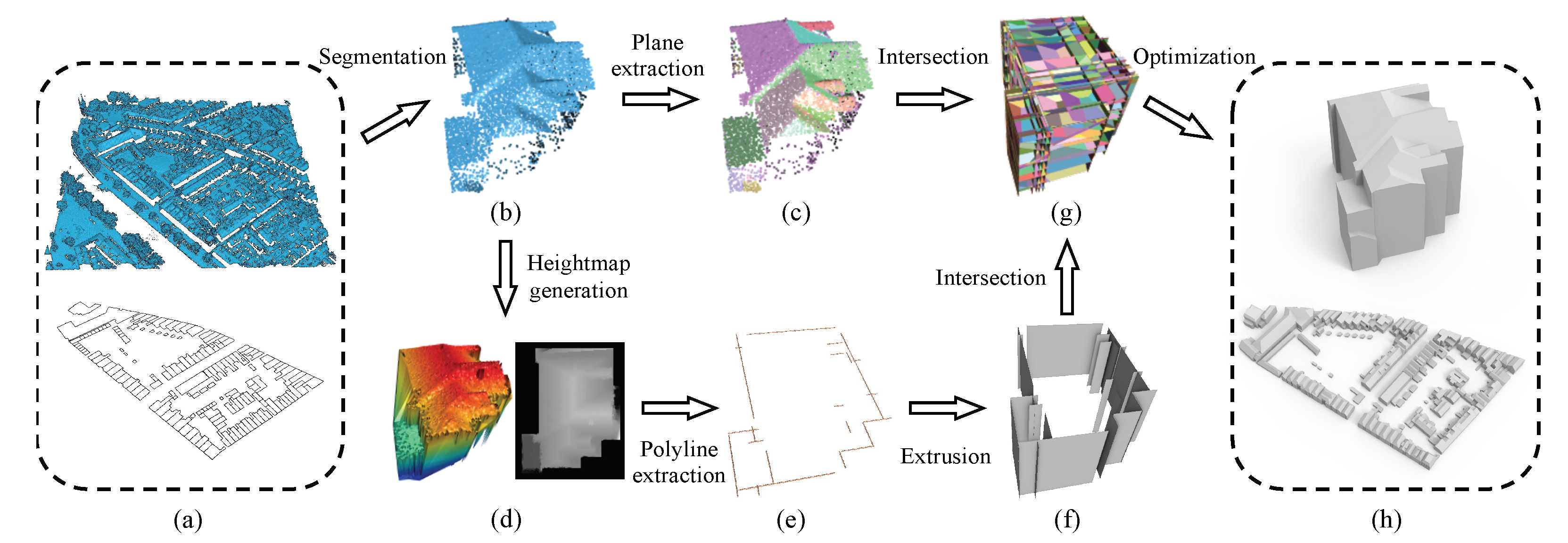
3.1. Overview
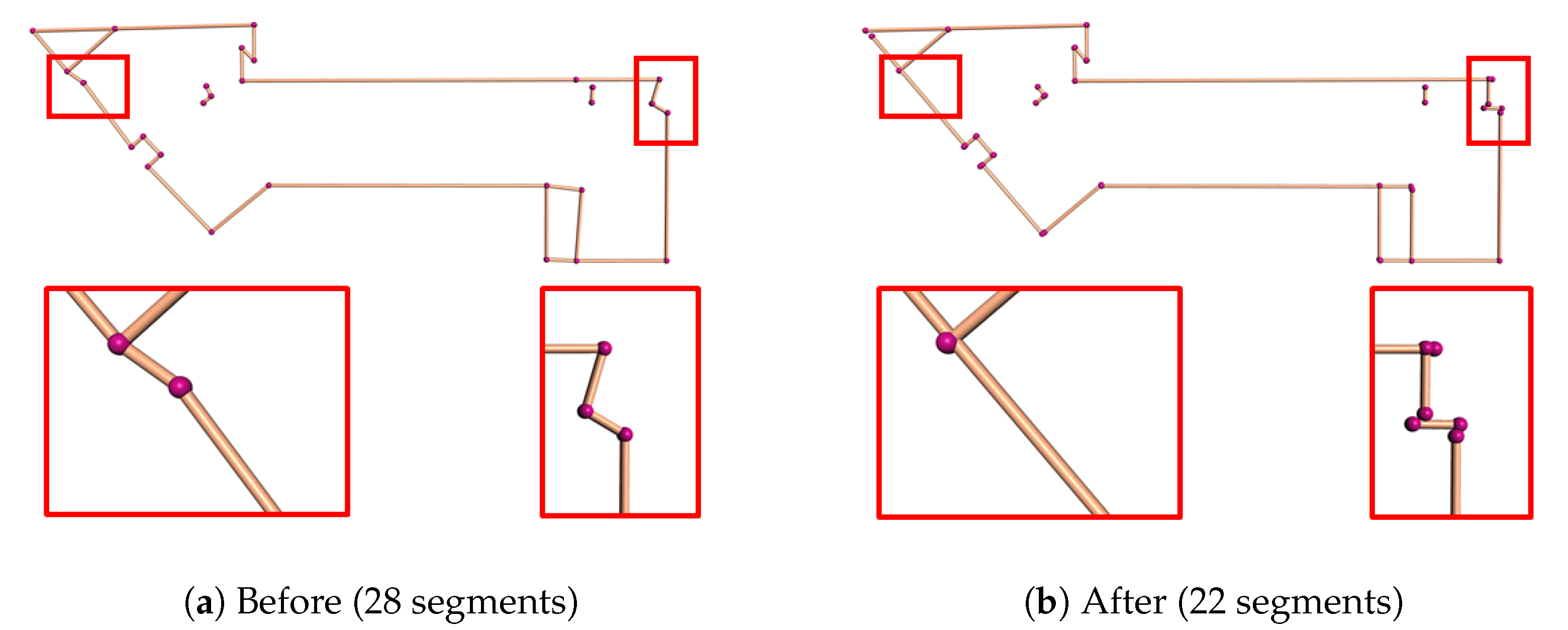
3.2. Inferring Vertical Planes
- The maximum Hausdorff distance from the simplified mesh to S is less than a distance threshold .
- The increase of the total transport cost [47] between S and is kept at a minimum.
3.3. Reconstruction
- Single-layer roof. This constraint ensures that the reconstructed 3D model of a real-world building has a single layer of roofs, which can be written as,where denotes the set of hypothesized faces that have overlap with face in the vertical direction.
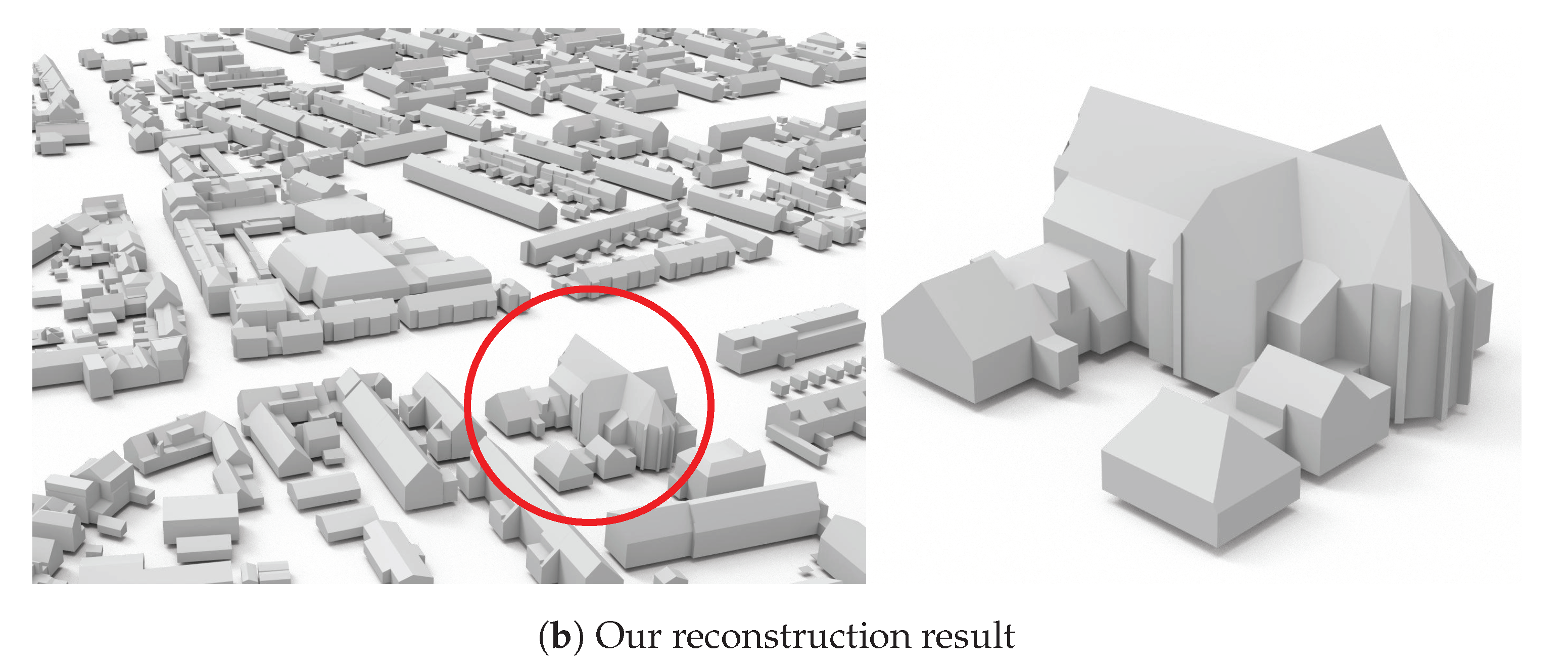
- Face prior. This constraint enforces that for all the derived faces from the same planar segment, the one with the highest confidence value is always selected as a prior. Here, the confidence of a face is measured by the number of its supporting points. This constraint can be simply written aswhere is the variable whose value denotes the status of the most confident face of a planar segment. This constraint resolves ambiguities if two hypothesized faces are near coplanar and close to each other, which preserves finer geometric details. The effect of this constraint is demonstrated in Figure 4.
4. Results and Evaluation
4.1. Test Datasets
- AHN3 [21]. An openly available country-wide airborne LiDAR point cloud dataset covering the entire Netherlands, with an average point density of 8 points/m. The corresponding footprints of the buildings are obtained from the Register of Buildings and Addresses (BAG) [51]. The geometry of footprint is acquired from aerial photos and terrestrial measurements with an accuracy of 0.3 m. The polygons in the BAG represent the outlines of buildings as their outer walls seen from above, which are slightly different from footprints. We still use ‘footprint’ in this paper.
- DALES [52]. A large-scale aerial point cloud dataset consisting of forty scenes spanning an area of 10 km, with instance labels of 6 k buildings. The data was collected using a Riegl Q1560 dual-channel system with a flight altitude of 1300 m above ground and a speed of 72 m/s. Each area was collected by a minimum of 5 laser pulses per meter in four directions. The LiDAR swaths were calibrated using the BayesStripAlign 2.0 software and registered, taking both relative and absolute errors into account and correcting for altitude and positional errors. The average point density is 50 points/m. No footprint data is available in this dataset.
- Vaihingen [53]. An airborne LiDAR point cloud dataset published by ISPRS, which has been widely used in semantic segmentation and reconstruction of urban scenes. The data were obtained using a Leica ALS50 system with 45° field of view and a mean flying height above ground of 500 m. The average strip overlap is 30% and multiple pulses were recorded. The point cloud was pre-processed to compensate for systematic offsets between the strips. We use in our experiments a training set that contains footprint information and covers an area of 399 m × 421 m with 753 k points. The average point density is 4 points/m.
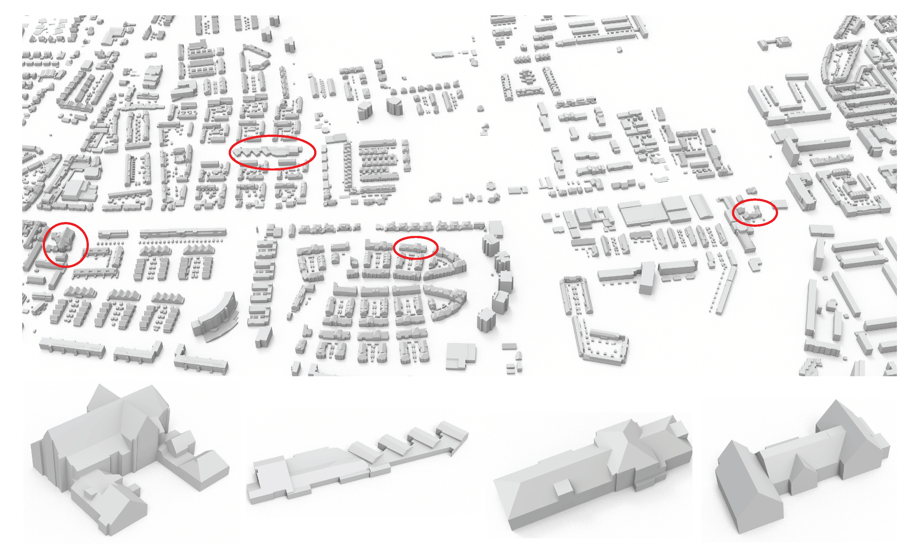
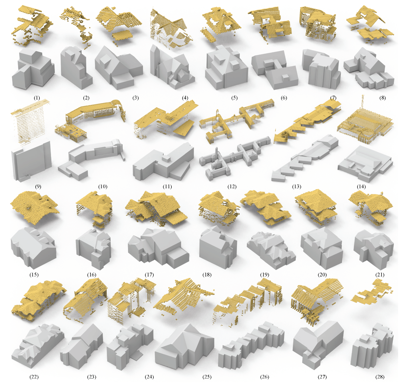
4.2. Reconstruction Results
4.3. Parameters
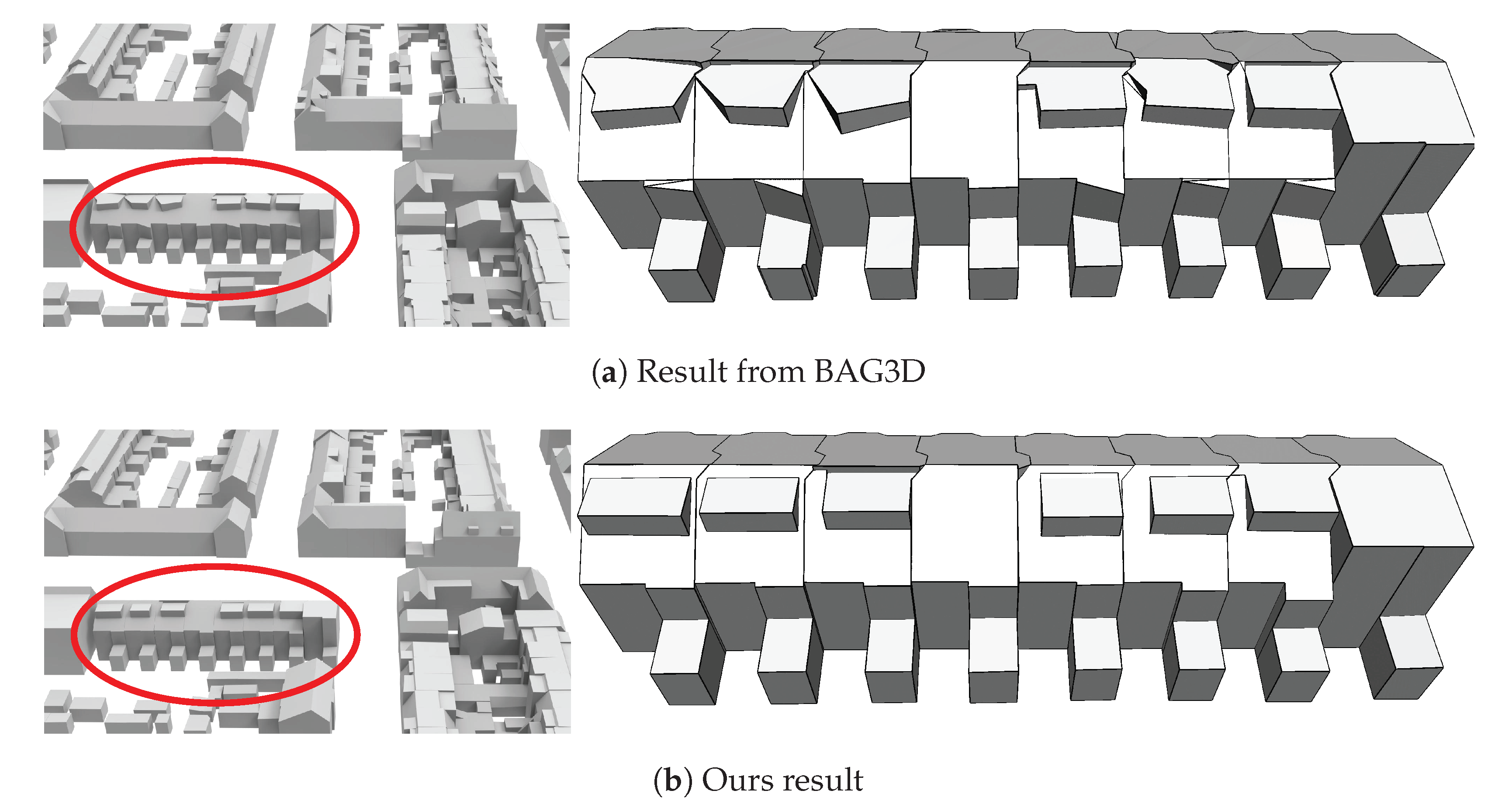
4.4. Comparisons
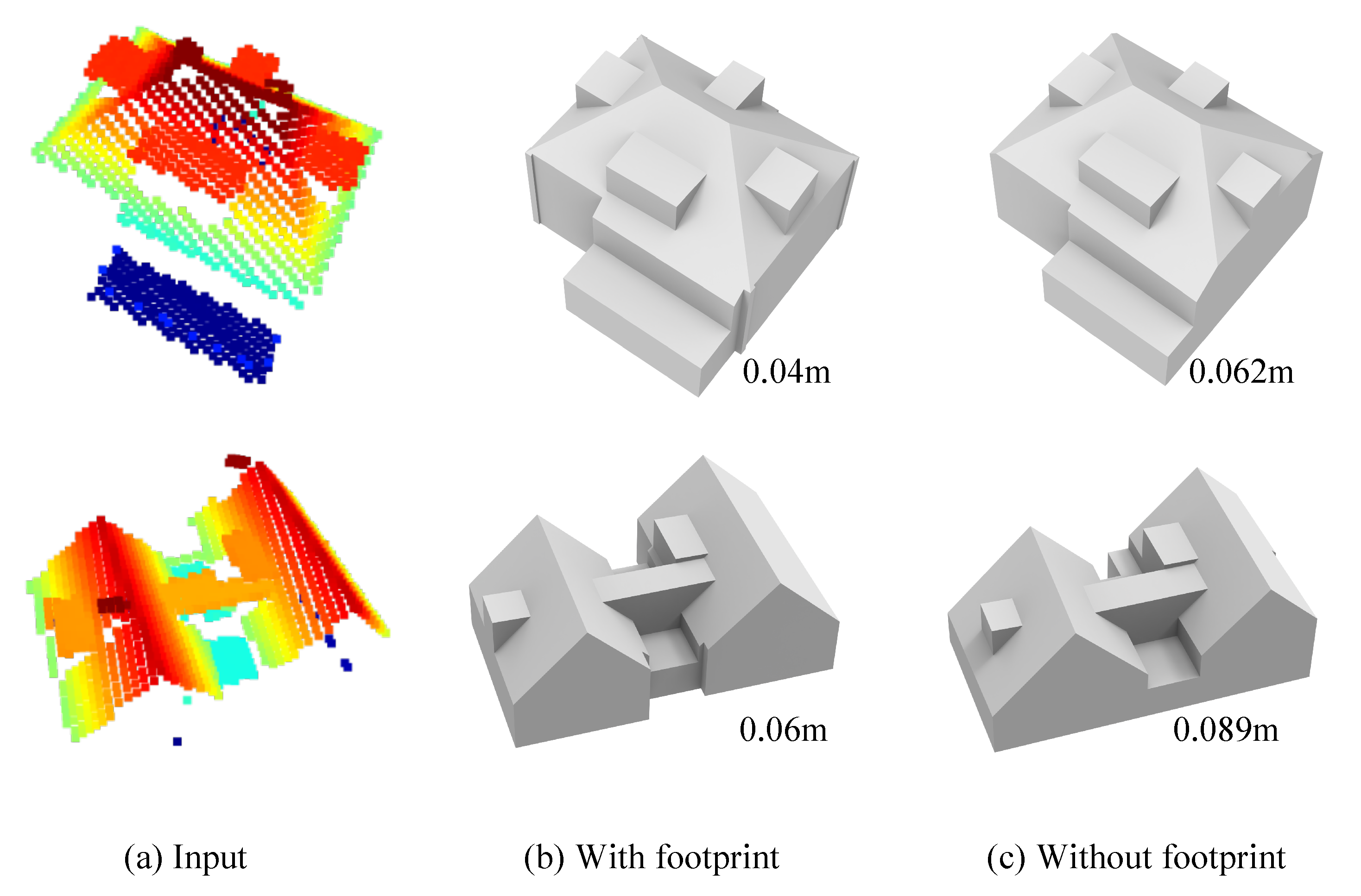
4.5. With vs. Without Footprint
4.6. Reconstruction Using Point Clouds with Vertical Planes
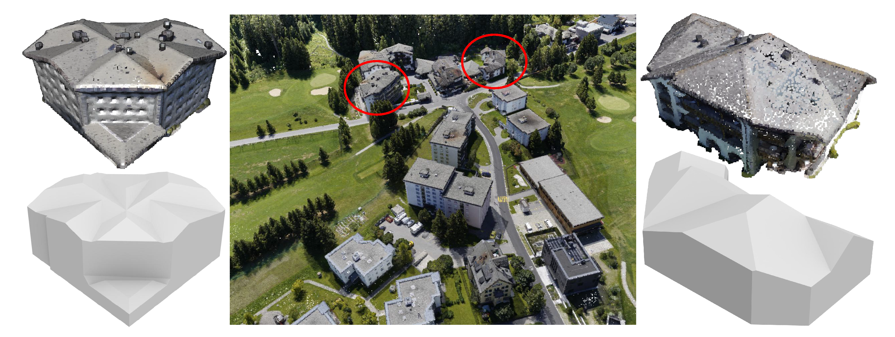
4.7. Limitations

5. Conclusions and Future Work
Author Contributions
Funding
Data Availability Statement
Acknowledgments
Conflicts of Interest
Abbreviations
| LiDAR | Light Detection and Ranging |
| TIN | Triangular Irregular Network |
| RMSE | Root Mean Square Error |
Appendix A. The Complete Formulation
- Data fitting. It is defined to measure how well the final model (i.e., the assembly of the chosen faces) fits to the input point cloud,where is the number of points in the point cloud. measures the number of points that are -close to a face , and denotes the binary status of the face (1 for selected and 0 otherwise). denotes the total number of hypothesized faces.
- Model complexity. To avoid defects introduced by noise and outliers, this term is introduced to encourage large planar structures,where denotes the total number of pairwise intersections in the hypothesized face set. is an indicator function denoting if choosing two faces connected by an edge results in a sharp edge in the final model (1 for sharp and 0 otherwise).
- Roof preference. We have observed in rare cases that a building in aerial point clouds may demonstrate more than one layer of roofs, e.g., semi-transparent or overhung roofs. In such a case, we assume a higher roof face is preferable to the ones underneath. We formulate this preference as an additional roof preference energy term,where denotes the Z coordinate of the centroid of a face . and are, respectively, the highest and lowest Z coordinates of the building points.
References
- Yao, Z.; Nagel, C.; Kunde, F.; Hudra, G.; Willkomm, P.; Donaubauer, A.; Adolphi, T.; Kolbe, T.H. 3DCityDB—A 3D geodatabase solution for the management, analysis, and visualization of semantic 3D city models based on CityGML. Open Geospat. Data Softw. Stand. 2018, 3, 1–26. [Google Scholar] [CrossRef] [Green Version]
- Zhivov, A.M.; Case, M.P.; Jank, R.; Eicker, U.; Booth, S. Planning tools to simulate and optimize neighborhood energy systems. In Green Defense Technology; Springer: Dordrecht, The Netherlands, 2017; pp. 137–163. [Google Scholar]
- Stoter, J.; Peters, R.; Commandeur, T.; Dukai, B.; Kumar, K.; Ledoux, H. Automated reconstruction of 3D input data for noise simulation. Comput. Environ. Urban Syst. 2020, 80, 101424. [Google Scholar] [CrossRef]
- Widl, E.; Agugiaro, G.; Peters-Anders, J. Linking Semantic 3D City Models with Domain-Specific Simulation Tools for the Planning and Validation of Energy Applications at District Level. Sustainability 2021, 13, 8782. [Google Scholar] [CrossRef]
- Cappelle, C.; El Najjar, M.E.; Charpillet, F.; Pomorski, D. Virtual 3D city model for navigation in urban areas. J. Intell. Robot. Syst. 2012, 66, 377–399. [Google Scholar] [CrossRef]
- Kargas, A.; Loumos, G.; Varoutas, D. Using different ways of 3D reconstruction of historical cities for gaming purposes: The case study of Nafplio. Heritage 2019, 2, 1799–1811. [Google Scholar] [CrossRef] [Green Version]
- Nan, L.; Sharf, A.; Zhang, H.; Cohen-Or, D.; Chen, B. Smartboxes for interactive urban reconstruction. In ACM Siggraph 2010 Papers; ACM: New Yrok, NY, USA, 2010; pp. 1–10. [Google Scholar]
- Nan, L.; Jiang, C.; Ghanem, B.; Wonka, P. Template assembly for detailed urban reconstruction. In Computer Graphics Forum; Wiley Online Library: Zurich, Switzerland, 2015; Volume 34, pp. 217–228. [Google Scholar]
- Zhou, Q.Y. 3D Urban Modeling from City-Scale Aerial LiDAR Data; University of Southern California: Los Angeles, CA, USA, 2012. [Google Scholar]
- Haala, N.; Rothermel, M.; Cavegn, S. Extracting 3D urban models from oblique aerial images. In Proceedings of the 2015 Joint Urban Remote Sensing Event (JURSE), Lausanne, Switzerland, 30 March–1 April 2015; pp. 1–4. [Google Scholar]
- Verdie, Y.; Lafarge, F.; Alliez, P. LOD generation for urban scenes. ACM Trans. Graph. 2015, 34, 30. [Google Scholar] [CrossRef] [Green Version]
- Li, M.; Nan, L.; Smith, N.; Wonka, P. Reconstructing building mass models from UAV images. Comput. Graph. 2016, 54, 84–93. [Google Scholar] [CrossRef] [Green Version]
- Buyukdemircioglu, M.; Kocaman, S.; Isikdag, U. Semi-automatic 3D city model generation from large-format aerial images. ISPRS Int. J.-Geo-Inf. 2018, 7, 339. [Google Scholar] [CrossRef] [Green Version]
- Bauchet, J.P.; Lafarge, F. City Reconstruction from Airborne Lidar: A Computational Geometry Approach. In Proceedings of the 3D GeoInfo 2019—14thConference 3D GeoInfo, Singapore, 26–27 September 2019. [Google Scholar]
- Li, M.; Rottensteiner, F.; Heipke, C. Modelling of buildings from aerial LiDAR point clouds using TINs and label maps. ISPRS J. Photogramm. Remote Sens. 2019, 154, 127–138. [Google Scholar] [CrossRef]
- Ledoux, H.; Biljecki, F.; Dukai, B.; Kumar, K.; Peters, R.; Stoter, J.; Commandeur, T. 3dfier: Automatic reconstruction of 3D city models. J. Open Source Softw. 2021, 6, 2866. [Google Scholar] [CrossRef]
- Zhou, X.; Yi, Z.; Liu, Y.; Huang, K.; Huang, H. Survey on path and view planning for UAVs. Virtual Real. Intell. Hardw. 2020, 2, 56–69. [Google Scholar] [CrossRef]
- Qi, C.R.; Su, H.; Mo, K.; Guibas, L.J. Pointnet: Deep learning on point sets for 3d classification and segmentation. In Proceedings of the IEEE Conference on Computer Vision and Pattern Recognition, Honolulu, HI, USA, 21–26 July 2017; pp. 652–660. [Google Scholar]
- Thomas, H.; Qi, C.R.; Deschaud, J.E.; Marcotegui, B.; Goulette, F.; Guibas, L.J. Kpconv: Flexible and deformable convolution for point clouds. In Proceedings of the IEEE/CVF International Conference on Computer Vision, Seoul, Korea, 27 October–2 November 2019; pp. 6411–6420. [Google Scholar]
- Nan, L.; Wonka, P. PolyFit: Polygonal Surface Reconstruction from Point Clouds. In Proceedings of the IEEE International Conference on Computer Vision, Venice, Italy, 22–29 October 2017. [Google Scholar]
- AHN3. Actueel Hoogtebestand Nederland (AHN). 2018. Available online: https://www.pdok.nl/nl/ahn3-downloads (accessed on 13 November 2021).
- Fischler, M.A.; Bolles, R.C. Random sample consensus: A paradigm for model fitting with applications to image analysis and automated cartography. Commun. ACM 1981, 24, 381–395. [Google Scholar] [CrossRef]
- Schnabel, R.; Wahl, R.; Klein, R. Efficient RANSAC for point-cloud shape detection. In Computer Graphics Forum; Wiley Online Library: Oxford, UK, 2007; Volume 26, pp. 214–226. [Google Scholar]
- Zuliani, M.; Kenney, C.S.; Manjunath, B. The multiransac algorithm and its application to detect planar homographies. In Proceedings of the IEEE International Conference on Image Processing 2005, Genova, Italy, 14 September 2005; Volume 3, p. III-153. [Google Scholar]
- Rabbani, T.; Van Den Heuvel, F.; Vosselmann, G. Segmentation of point clouds using smoothness constraint. Int. Arch. Photogramm. Remote Sens. Spat. Inf. Sci. 2006, 36, 248–253. [Google Scholar]
- Sun, S.; Salvaggio, C. Aerial 3D building detection and modeling from airborne LiDAR point clouds. IEEE J. Sel. Top. Appl. Earth Obs. Remote Sens. 2013, 6, 1440–1449. [Google Scholar] [CrossRef]
- Chen, D.; Wang, R.; Peethambaran, J. Topologically aware building rooftop reconstruction from airborne laser scanning point clouds. IEEE Trans. Geosci. Remote Sens. 2017, 55, 7032–7052. [Google Scholar] [CrossRef]
- Meng, X.; Wang, L.; Currit, N. Morphology-based building detection from airborne LIDAR data. Photogramm. Eng. Remote Sens. 2009, 75, 437–442. [Google Scholar] [CrossRef]
- Douglas, D.H.; Peucker, T.K. Algorithms for the reduction of the number of points required to represent a digitized line or its caricature. Cartogr. Int. J. Geogr. Inf. Geovis. 1973, 10, 112–122. [Google Scholar] [CrossRef] [Green Version]
- Zhang, K.; Yan, J.; Chen, S.C. Automatic construction of building footprints from airborne LIDAR data. IEEE Trans. Geosci. Remote Sens. 2006, 44, 2523–2533. [Google Scholar] [CrossRef] [Green Version]
- Xiong, B.; Elberink, S.O.; Vosselman, G. Footprint map partitioning using airborne laser scanning data. ISPRS Ann. Photogramm. Remote Sens. Spat. Inf. Sci. 2016, 3, 241–247. [Google Scholar] [CrossRef] [Green Version]
- Zhou, Q.Y.; Neumann, U. Fast and extensible building modeling from airborne LiDAR data. In Proceedings of the 16th ACM SIGSPATIAL International Conference on Advances in Geographic Information Systems, Irvine, CA, USA, 5–7 November 2008; pp. 1–8. [Google Scholar]
- Dorninger, P.; Pfeifer, N. A comprehensive automated 3D approach for building extraction, reconstruction, and regularization from airborne laser scanning point clouds. Sensors 2008, 8, 7323–7343. [Google Scholar] [CrossRef] [Green Version]
- Lafarge, F.; Mallet, C. Creating large-scale city models from 3D-point clouds: A robust approach with hybrid representation. Int. J. Comput. Vis. 2012, 99, 69–85. [Google Scholar] [CrossRef]
- Xiao, Y.; Wang, C.; Li, J.; Zhang, W.; Xi, X.; Wang, C.; Dong, P. Building segmentation and modeling from airborne LiDAR data. Int. J. Digit. Earth 2015, 8, 694–709. [Google Scholar] [CrossRef]
- Yi, C.; Zhang, Y.; Wu, Q.; Xu, Y.; Remil, O.; Wei, M.; Wang, J. Urban building reconstruction from raw LiDAR point data. Comput.-Aided Des. 2017, 93, 1–14. [Google Scholar] [CrossRef]
- Zhou, Q.Y.; Neumann, U. 2.5 d dual contouring: A robust approach to creating building models from aerial lidar point clouds. In European Conference on Computer Vision; Springer: Cham, Switzerland, 2010; pp. 115–128. [Google Scholar]
- Zhou, Q.Y.; Neumann, U. 2.5 D building modeling with topology control. In Proceedings of the CVPR 2011, Colorado Springs, CO, USA, 20–25 June 2011; pp. 2489–2496. [Google Scholar]
- Chauve, A.L.; Labatut, P.; Pons, J.P. Robust piecewise-planar 3D reconstruction and completion from large-scale unstructured point data. In Proceedings of the 2010 IEEE Computer Society Conference on Computer Vision and Pattern Recognition, San Francisco, CA, USA, 13–18 June 2010; pp. 1261–1268. [Google Scholar]
- Lafarge, F.; Descombes, X.; Zerubia, J.; Pierrot-Deseilligny, M. Structural approach for building reconstruction from a single DSM. IEEE Trans. Pattern Anal. Mach. Intell. 2008, 32, 135–147. [Google Scholar] [CrossRef] [Green Version]
- Xiong, B.; Elberink, S.O.; Vosselman, G. A graph edit dictionary for correcting errors in roof topology graphs reconstructed from point clouds. ISPRS J. Photogramm. Remote Sens. 2014, 93, 227–242. [Google Scholar] [CrossRef]
- Li, M.; Wonka, P.; Nan, L. Manhattan-world Urban Reconstruction from Point Clouds. In European Conference on Computer Vision; Springer: Cham, Switzerland, 2016. [Google Scholar]
- Bauchet, J.P.; Lafarge, F. Kinetic shape reconstruction. ACM Trans. Graph. (TOG) 2020, 39, 1–14. [Google Scholar] [CrossRef]
- Fang, H.; Lafarge, F. Connect-and-Slice: An hybrid approach for reconstructing 3D objects. In Proceedings of the IEEE/CVF Conference on Computer Vision and Pattern Recognition, Seattle, WA, USA, 14–19 June 2020; pp. 13490–13498. [Google Scholar]
- Huang, H.; Brenner, C.; Sester, M. A generative statistical approach to automatic 3D building roof reconstruction from laser scanning data. ISPRS J. Photogramm. Remote Sens. 2013, 79, 29–43. [Google Scholar] [CrossRef]
- Canny, J. A computational approach to edge detection. IEEE Trans. Pattern Anal. Mach. Intell. 1986, PAMI-8, 679–698. [Google Scholar] [CrossRef]
- De Goes, F.; Cohen-Steiner, D.; Alliez, P.; Desbrun, M. An optimal transport approach to robust reconstruction and simplification of 2D shapes. In Computer Graphics Forum; Wiley Online Library: Oxford, UK, 2011; Volume 30, pp. 1593–1602. [Google Scholar]
- Li, Y.; Wu, B. Relation-Constrained 3D Reconstruction of Buildings in Metropolitan Areas from Photogrammetric Point Clouds. Remote Sens. 2021, 13, 129. [Google Scholar] [CrossRef]
- Schubert, E.; Sander, J.; Ester, M.; Kriegel, H.P.; Xu, X. DBSCAN revisited, revisited: Why and how you should (still) use DBSCAN. ACM Trans. Database Syst. (TODS) 2017, 42, 1–21. [Google Scholar] [CrossRef]
- CGAL Library. CGAL User and Reference Manual, 5.0.2 ed.; CGAL Editorial Board: Valbonne, French, 2020. [Google Scholar]
- BAG. Basisregistratie Adressen en Gebouwen (BAG). 2019. Available online: https://bag.basisregistraties.overheid.nl/datamodel (accessed on 13 November 2021).
- Varney, N.; Asari, V.K.; Graehling, Q. DALES: A large-scale aerial LiDAR data set for semantic segmentation. In Proceedings of the IEEE/CVF Conference on Computer Vision and Pattern Recognition Workshops, Seattle, WA, USA, 14–19 June 2020; pp. 186–187. [Google Scholar]
- Rottensteiner, F.; Sohn, G.; Jung, J.; Gerke, M.; Baillard, C.; Benitez, S.; Breitkopf, U. The ISPRS benchmark on urban object classification and 3D building reconstruction. ISPRS Ann. Photogramm. Remote Sens. Spat. Inf. Sci. I-3 2012, 1, 293–298. [Google Scholar] [CrossRef] [Green Version]
- Kazhdan, M.; Bolitho, M.; Hoppe, H. Poisson surface reconstruction. In Proceedings of the Fourth Eurographics Symposium on Geometry Processing, Cagliari, Italy, 26–28 June 2006; Volume 7. [Google Scholar]
- 3D BAG (v21.09.8). 2021. Available online: https://3dbag.nl/en/viewer (accessed on 13 November 2021).
- Can, G.; Mantegazza, D.; Abbate, G.; Chappuis, S.; Giusti, A. Semantic segmentation on Swiss3DCities: A benchmark study on aerial photogrammetric 3D pointcloud dataset. Pattern Recognit. Lett. 2021, 150, 108–114. [Google Scholar] [CrossRef]


| Dataset | Model | #Points | #Faces | RMSE (m) | Time (s) |
|---|---|---|---|---|---|
| AHN3 | (1) | 732 | 23 | 0.07 | 3 |
| (2) | 532 | 42 | 0.12 | 4 | |
| (3) | 1165 | 31 | 0.04 | 3 | |
| (4) | 20,365 | 127 | 0.15 | 62 | |
| (5) | 1371 | 48 | 0.04 | 5 | |
| (6) | 1611 | 45 | 0.06 | 4 | |
| (7) | 3636 | 68 | 0.21 | 18 | |
| (8) | 2545 | 52 | 0.04 | 8 | |
| (9) | 15,022 | 63 | 0.11 | 28 | |
| (10) | 23,654 | 262 | 0.26 | 115 | |
| (11) | 13,269 | 102 | 0.11 | 34 | |
| (12) | 155,360 | 1520 | 0.09 | 2520 | |
| (13) | 24,027 | 176 | 0.24 | 141 | |
| (14) | 28,522 | 227 | 0.15 | 78 | |
| DALES | (15) | 8662 | 39 | 0.04 | 11 |
| (16) | 11,830 | 73 | 0.1 | 8 | |
| (17) | 10,673 | 47 | 0.07 | 7 | |
| (18) | 7594 | 33 | 0.07 | 14 | |
| (19) | 13,060 | 278 | 0.05 | 145 | |
| (20) | 11,114 | 55 | 0.06 | 24 | |
| (21) | 8589 | 51 | 0.06 | 15 | |
| (22) | 18,909 | 282 | 0.08 | 86 | |
| Vaihingen | (23) | 7701 | 51 | 0.24 | 25 |
| (24) | 6845 | 99 | 0.12 | 8 | |
| (25) | 1007 | 24 | 0.11 | 2 | |
| (26) | 11,591 | 206 | 0.17 | 10 | |
| (27) | 4026 | 42 | 0.26 | 6 | |
| (28) | 5059 | 61 | 0.22 | 9 |
| Dataset | Method | #Faces | RMSE (m) | Time (s) |
|---|---|---|---|---|
| AHN3 | 2.5D DC [37] | 12,781 | 0.213 | 13 |
| PolyFit [20] | 1848 | 0.242 | 160 | |
| Ours | 2453 | 0.128 | 380 | |
| DALES | 2.5D DC [37] | 2297 | 0.204 | 10 |
| PolyFit [20] | 444 | 0.287 | 230 | |
| Ours | 583 | 0.184 | 670 | |
| Vaihingen | 2.5D DC [37] | 2695 | 0.168 | 6 |
| PolyFit [20] | 647 | 0.275 | 102 | |
| Ours | 798 | 0.157 | 212 |
| Region | #Points | #Building | RMSE (m) BAG3D | RMSE (m) Ours |
|---|---|---|---|---|
| (a) | 1,694,247 | 198 | 0.088 | 0.079 |
| (b) | 329,593 | 387 | 0.139 | 0.138 |
| (c) | 224,970 | 368 | 0.140 | 0.132 |
| (d) | 80,447 | 160 | 0.146 | 0.128 |
Publisher’s Note: MDPI stays neutral with regard to jurisdictional claims in published maps and institutional affiliations. |
© 2022 by the authors. Licensee MDPI, Basel, Switzerland. This article is an open access article distributed under the terms and conditions of the Creative Commons Attribution (CC BY) license (https://creativecommons.org/licenses/by/4.0/).
Share and Cite
Huang, J.; Stoter, J.; Peters, R.; Nan, L. City3D: Large-Scale Building Reconstruction from Airborne LiDAR Point Clouds. Remote Sens. 2022, 14, 2254. https://doi.org/10.3390/rs14092254
Huang J, Stoter J, Peters R, Nan L. City3D: Large-Scale Building Reconstruction from Airborne LiDAR Point Clouds. Remote Sensing. 2022; 14(9):2254. https://doi.org/10.3390/rs14092254
Chicago/Turabian StyleHuang, Jin, Jantien Stoter, Ravi Peters, and Liangliang Nan. 2022. "City3D: Large-Scale Building Reconstruction from Airborne LiDAR Point Clouds" Remote Sensing 14, no. 9: 2254. https://doi.org/10.3390/rs14092254
APA StyleHuang, J., Stoter, J., Peters, R., & Nan, L. (2022). City3D: Large-Scale Building Reconstruction from Airborne LiDAR Point Clouds. Remote Sensing, 14(9), 2254. https://doi.org/10.3390/rs14092254