Article

Combining Deep Semantic Edge and Object Segmentation for Large-Scale Roof-Part Polygon Extraction from Ultrahigh-Resolution Aerial Imagery

by
Wouter A. J. Van den Broeck
* and
Toon Goedemé
ESAT-PSI-EAVISE, KU Leuven, Jan Pieter De Nayerlaan 5, 2860 Sint-Katelijne-Waver, Belgium
*
Author to whom correspondence should be addressed.
Remote Sens. 2022, 14(19), 4722; https://doi.org/10.3390/rs14194722
Submission received: 30 June 2022 / Revised: 6 August 2022 / Accepted: 16 September 2022 / Published: 21 September 2022
(This article belongs to the Special Issue Remote Sensing Based Building Extraction II)

Abstract

:
The roofscape plays a vital role in the support of sustainable urban planning and development. However, availability of detailed and up-to-date information on the level of individual roof-part topology remains a bottleneck for reliable assessment of its present status and future potential. Motivated by the need for automation, the current state-of-the-art focuses on applying deep learning techniques for roof-plane segmentation from light-detection-and-ranging (LiDAR) point clouds, but fails to deliver on criteria such as scalability, spatial predictive continuity, and vectorization for use in geographic information systems (GISs). Therefore, this paper proposes a fully automated end-to-end workflow capable of extracting large-scale continuous polygon maps of roof-part instances from ultra-high-resolution (UHR) aerial imagery. In summary, the workflow consists of three main steps: (1) use a multitask fully convolutional network (FCN) to infer semantic roof-part edges and objects, (2) extract distinct closed shapes given the edges and objects, and (3) vectorize to obtain roof-part polygons. The methodology is trained and tested on a challenging dataset comprising of UHR aerial RGB orthoimagery (0.03 m GSD) and LiDAR-derived digital elevation models (DEMs) (0.25 m GSD) of three Belgian urban areas (including the famous touristic city of Bruges). We argue that UHR optical imagery may provide a competing alternative for this task over classically used LiDAR data, and investigate the added value of combining these two data sources. Further, we conduct an ablation study to optimize various components of the workflow, reaching a final panoptic quality of 54.8% (segmentation quality = 87.7%, recognition quality = 62.6%). In combination with human validation, our methodology can provide automated support for the efficient and detailed mapping of roofscapes.

Graphical Abstract

1. Introduction

As buildings cover a considerable area of the urban environment, the roofscape plays a vital role in supporting sustainable urban development [1]. Roofs hold a myriad of potential uses, including civic spaces, urban farms, rainwater harvesting, and solar power. Strategic design choices of the roofscape, such as material type and coverage, are therefore instrumental in regulating the urban energy budget, storm water management, and local food systems. For instance, popular incentives include installing solar panels to aid in achieving a net-zero energy consumption, thermal insulation to reduce building energy use and thus their carbon footprint, and green roofs to contribute to reducing traffic noise, improving air quality and urban biodiversity, and mitigating the urban heat island effect.
To assess the current status and future potential of the sustainable roofscape, accurate and up-to-date information on the spatial distribution and topology of rooftops is needed. Simple building contour maps can often be found from open-source databases (e.g., OpenStreetMap or local governments). However, more detailed maps of individual roofparts are lacking. We define a roof part here as a semantic instance within a larger roof complex, distinguishable from other roof parts by a difference in inclination, height, roof material, or any other kind of roof-part edge. Following this definition, we consider a roof part to be different from a roofplane, as a roofplane may, for instance, be constituted of different roof parts, e.g., neighboring houses in ribbon development may share the same roofplane that comprises different roof parts separated by gutters. Such more refined maps are needed to facilitate the construction of geographic information systems (GISs) linking attributes to the roof parts, including the surface area, inclination, position, roof material, thermal insulation, degradation state, and mounted objects (e.g., solar panels, air conditioners, satellite dishes), and would allow for better estimates of the solar photovoltaic and green potential of a roofscape. Since mapping roof parts for large areas is a tedious and time-consuming task, automated methodologies are necessary. However, to the best of our knowledge, no end-to-end methodology has yet been proposed for the efficient automated extraction of roof-part maps on a large scale.
Undeniably, deep learning has become the tool of choice for the automated supervised image analysis of airborne and spaceborne Earth observation (EO) imagery, be it for object detection, semantic segmentation, or instance segmentation [2]. Largely driven by data availability, the majority of research concerned with applying deep learning for rooftop mapping focuses on either (1) building footprint extraction from RGB (ortho-)images [3], sometimes combined with LiDAR-derived 2D height maps [4,5], or (2) roof-plane segmentation from LiDAR point clouds [6,7,8,9,10]. Research on the first application is predominantly propelled by well-known open-source datasets such as Vaihingen [11], the Inria Aerial Image Labelling Dataset [12] or the more recent SemCity Toulouse [13]. The scope of these studies is solely to segment complete rooftop instances and not individual roof parts that constitute the rooftops. The smaller body of research focusing on the second application uses smaller datasets, as LiDAR is more costly and complex to acquire than optical imagery. Arguably, this render LiDAR a suboptimal choice for large-scale high-resolution problem settings. Therefore, in this paper we compare using only LiDAR-derived height data (i.e., a digital elevation model (DEM)) with using only RGB orthoimagery, and show that, for our case, the latter outperformed the former. Additionally, we investigate the added value of combining these two data sources (RGB + DEM).
Furthermore, an increasing number of rooftop or roofplane extraction methodologies are recognizing the importance of having polygon maps as the workflow output as opposed to only providing the identified rooftops as pixel-based areas (i.e., a raster map) [14,15]. The difficulty with raster maps is that they require considerable storage memory, and are inconvenient for further processing and usage in a GIS. Hence, this paper also advocates that automated mapping approaches should target polygon maps as the workflow output rather than raster maps. This goes in hand with two crucial considerations. First, although segmentation algorithms are becoming increasingly accurate, they often cannot ensure closed object shapes, hence hampering the vectorization of the raster object [16]. Second, due to the patchwise processing of large EO imagery because of computational constraints, predictive spatial continuity is not always ensured. More specifically, it is obvious that methodologies that assume either a single object instance per image patch (e.g., a single building) or only a limited number of scattered instances are not applicable for large-scale roof-part extraction. As such, there is a need for paradigms that take these consideration into account.
Having identified some key requirements for large-scale roof-part polygon extraction, this paper proposes a workflow based on three steps: (1) use a deep neural network to predict roof-part objects and edges, (2) use a bottom–up clustering algorithm given the predicted edges to derive distinct closed shapes, and (3) vectorize and simplify the roof-part shapes. For Step 1, we opted for a semantic segmentation approach using a fully convolutional network (FCN). We did not use a detection-based instance segmentation method (i.e., using bounding boxes), such as the famous mask R-CNN [17], because they have difficulty with highly clustered instances, which is evidently the case for urban roofscapes. Therefore, the emphasis of the workflow lies on finding roof-part edges rather than roof-part objects. To this end, we briefly review the related work focusing on using FCNs for rooftop edge segmentation. The overall objective of these studies is to optimize semantic object and edge predictions by designing specific FCN architectures or training loss functions that explicitly account for both targets. For example, Marmanis et al. (2018) integrated a separate edge detector (holistically nested edge detection (HED)) into their semantic segmentation model to build in semantic boundary awareness [18]. Wu et al. (2018) proposed a boundary regulated network (BR-Net) to simultaneously perform building segmentation and outline extraction on the basis of a shared feature representation and a multilabel optimization approach [19]. Diakogiannis et al. (2020) also built on the idea of multitask inference and created ResUnet-a, a FCN that simultaneously outputs a semantic object mask, edge mask, object center distance map, and an HSV colored reconstruction of the input [20]. To promote edge connectivity and clear object boundaries, Xia et al. (2021) designed specific edge guidance modules and applied multiscale supervision for training their network (DDLNet) [16]. Additionally, they used a multilabel target approach concatenating the edge prediction as a feature map for predicting the semantic objects. Next, a number of studies proposed custom loss functions to improve edge and object-boundary predictions, of which most are weighted flavors of the Dice loss, cross-entropy loss, or combinations of the latter [14,21]. Here, the chief consideration is to cope with class imbalance, as the number of edge pixels is typically a number of magnitudes lower than the number of non-edge pixels. Further, some works address the problem of building instance segmentation from a different angle by combining FCNs with other deep-learning paradigms to predict building corners as key points, which can more easily be processed into regular polygons [22,23]. Lastly, an alternative direction is to train directly on extracting polygon coordinates. For example, Chen et al. (2020) proposed a modeling framework for vectorized building outline extraction using a combination of FCN-based segmentation and a modified PointNet to learn shape priors and predict polygon vertex deformation [24].
However, the aforementioned studies focused on complete roof extraction and not on individual roof-part extraction. Moreover, no existing framework could be readily applied to our application as they failed to fulfil at least one of our identified criteria, i.e., (i) scalable to large areas, (ii) predictive spatial continuity, and (iii) polygon-oriented. Therefore, the novelty of this paper is manifold: (i) we propose a fully automated workflow for the extraction of individual roof parts on a large scale; (ii) we suggest a multiclass FCN approach for combined semantic edge and object prediction, as opposed to the more common multilabel approach; (iii) spatial predictive continuity is taken into account by saving intermediate output mosaics; and (iv) the methodology is polygon-oriented, i.e., the FCN ground truth is generated on the fly on the basis of polygon annotations, the workflow output is a polygon map, and the quality assessment is polygon-based. The methodology was trained and tested on a new challenging dataset comprising of UHR aerial RGB orthoimagery (0.03 m GSD) and LiDAR-derived DEMs (0.25 m GSD) of three Belgian urban areas (including the famous touristic city of Bruges). We conducted an ablation study to optimize various components of the workflow, reaching a final panoptic quality of 54.8% (segmentation quality of 87.7% and recognition quality of 62.6%). Lastly, we highlight some current shortcomings, potential improvements, and future opportunities.

2. Materials and Methods

2.1. Study Area and Dataset

The study area under consideration is the region of Flanders, i.e., the northern part of Belgium (Figure 1). Geographically, Flanders is an agriculturally fertile and densely populated region with little to no relief. The landscape is predominantly characterized by cropland (ca. 31%), agricultural grassland (ca. 20%), residential areas (ca. 13%), and tree cover or forests (ca. 10%). Another ca. 15% is covered by human infrastructure for transport, services, built-op areas, industry, agriculture, and airports [25]. The cities and villages are mainly organized as dense smaller city centers with little to no high-rise buildings and surrounding ribbon development. The building architecture and structure, and hence the rooftop appearance, are highly diverse.
To develop and test our methodology, we selected three municipalities within Flanders to serve as training, validation, and test regions: Brugge, Jabbeke, and Lokeren, respectively (Figure 1). For each of the three towns, the following data were available: (1) an aerial RGB orthophoto with ultrahigh resolution of 0.03 m GSD stored as an ERDAS JPEG2000 uint8 compressed file. To give a notion of the magnitude, the Lokeren orthophoto, covering 3.65 km 2 , has an image resolution of 320,716 × 297,190 pixels. The used coordinate reference system (CRS) was the Belgian Lambert 72 (EPSG:31370). (2) A digital elevation model (DEM) of 0.25 m GSD stored as float32 GeoTIFF. (3) Polygon labels delineating all distinct roof parts within the three considered regions, stored as GeoJSON files. The labels were generated by (nonexpert) human annotators on the basis of the visual interpretation of the RGB orthophotos. Inevitably, the latter gives rise to some degree of interpretive variability and erroneous labels. Nonetheless, visual inspection confirmed that the annotations were of sufficient quality for training and evaluating our methodology.
Table 1 provides a quantitative overview of the dataset. Figure 2 and Figure 3 further show the distribution of roof-part types and roof-part sizes for the three partitions, respectively. The latter reflect that Brugge (training set) has a highly compact, complex, and densely clustered rooftop structure, i.e., approximately half of the total area (0.72 km 2 ) is covered by roofs (0.34 km 2 ), with strongly right-skewed roof-part size distribution and a median roof size of only 7.1 m 2 . This feature of many different examples on a small area is advantageous, as it allows for faster model training (see Section 2.3.3). In contrast, Lokeren (test set) is more characterized by a combination of densely clustered roofs, isolated houses, and some very large roofs. Further, Lokeren has approximately the same number of roof parts as Brugge (ca. 27 × 10 3 ), but spread out over a region almost five times as large. As such, this allows for evaluating the model on unseen scenery and areas without roofs, rendering our test set truly honest and challenging. Lastly, Jabbeke (validation set) is a smaller town with suburban appearance. It was used for the validation of the performance and generalizability of the models during training.

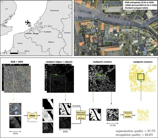
2.2. Workflow Overview

Here, we elaborate on our proposed workflow for large-scale roof-part polygon generation given UHR orthoimagery (Figure 4). In general, the workflow consisted of three main steps: (1) A trained FCN was used to infer semantic roof-part edges and objects. (2) Distinct closed shapes were extracted given the edges and objects. (3) The closed shapes were vectorized to obtain roof-part polygons. As depicted in Figure 4, each step was computationally constrained by a certain patch size (PS), i.e., the maximal image resolution that could be algorithmically processed in terms of time and/or memory. However, in contrast to natural imagery, EO imagery is spatially continuous. Therefore, it is important to ensure the continuity of the overall output despite patchwise processing. As a larger PS corresponds to a smoother overall output, saving intermediate results allows for setting the PSs to a different optimal value for each step. Usually, P S F C N < P S C S E < P S V E C , where P S F C N is the input patch size of the FCN model, P S C S E of the closed shape extraction step, and P S V E C of the vectorizing step. Each of the three steps is described in more detail in the subsequent sections.

2.3. Semantic Edge and Object Segmentation

As a first step, we used an FCN to learn a function Y ^ = f ( X , θ ) with parameters θ to map an input image X R [ 0 , 1 ] C i × H × W to predicted semantic probability maps Y ^ R [ 0 , 1 ] C o × H × W , with C i being the number of input channels, C o the number of output channels, H the image height, and W the image width. Each pixel in the output Y ^ represents the confidence with which the corresponding pixel in the input X belongs to a certain semantic class, such as, in our case, roof vs. non-roof and/or roof edge vs. non-roof edge. We compared three paradigms for deriving roof-object and roof-edge probability maps (Figure 5): (i) two independent FCNs with binary output; (ii) a single FCN with multilabel output, i.e., each pixel could belong to multiple classes; and (iii) a single FCN with multiclass output, i.e., each pixel could belong to only one class. Below, we briefly describe the FCN architecture, and the training and validation procedure.

2.3.1. FCN Architectures

The used FCN is the well-known UNet architecture [26]. To date, it remains the standard for semantic segmentation of EO imagery [2]. More specifically, we use a UNet with an EfficientNet-B5 [27] 5-stage encoder ( H = W = 2 x 2 x / 5 ) pretrained on Imagenet [28], and a decoder with batch normalization and spatial and channel squeeze & excitation (scSE) attention modules after every decoder stage [29], as implemented in the pytorch-segmentation-models Python package [30]. The input of the FCN is a 1-channel DEM ( C i = 1 ), 3-channel RGB ( C i = 3 ) or 4-channel RGB + DEM ( C i = 4 ) image patch. The used P S F C N is H = W = 1024 pix, corresponding to a ground resolution of ∼30 × 30 m 2 . This is the largest PS that could fit into GPU memory during FCN training. The output of the FCN is different for each of the three approaches (Figure 5). For the double binary case, the output is twice a single channel ( C o = 1 : roof object; C o = 1 : roof edge) with pixelwise sigmoid activation to obtain the probability maps. For the single multilabel case, the output is two-channeled ( C o = 2 : roof object, roof edge) with sigmoid activation. For the multiclass case, the output is three-channeled ( C o = 3 : roof object, roof edge, and neither) with softmax activation over the channels to ensure mutual exclusiveness. To save memory, the predicted probability patches can simply be saved into the complete output mosaic as integer maps: X u i n t 8 = X f l o a t × 255 .

2.3.2. Data Preprocessing

The models are trained by feeding them batches of image patches and the corresponding ground truth. The ground truth is generated on the fly by rasterizing the polygons occurring within the input patches to binary maps Y B C o × H × W . To obtain a roof-object target, the full polygon surface is rasterized, while to obtain a roof-edge target, the polygons are first converted into their line-string format and subsequently dilated by a certain number of pixels (in the vector space), again resulting in a polygon that is then rasterized. For the multiclass model, the roof-edge channel is subtracted from the roof-object channel, and the background channel is obtained as the logical negation of the roof object and edge channels.
To match input dimensions, the DEM is bilinearly upsampled to the resolution of the RGB. Further, DEM values are transformed by clipping all values to the range of 0–30 m and subsequently rescaling them to the 0–1 domain: X D E M , [ 0 , 1 ] = max ( 0 , min ( 30 , X D E M ) ) / 30 . This range was arbitrarily chosen, as most buildings in the considered study area are smaller than 30 m, and height values cannot be negative.
Image augmentation techniques were used for the training set, including random flipping, minor (HSV) color variations, jitter (random small translation of the considered patch), and an overlap of 128 pix between adjacent patches. Moreover, to balance and limit the training and validation sets, only patches with occurrence of roofs were included. In the test set, patches without roofs were also included. This resulted in 982 training patches (759 in the case of no overlap), 187 validation patches, and 3865 test patches.

2.3.3. FCN Training

All FCN models were trained for 30 epochs using the Adam optimizer, a fixed learning rate of 2 × 10 4 , and a batch size of 3. The used hardware was an NVIDIA Tesla V100 GPU with 32 GB memory (CUDA 11.0). The model architectures, and training and validation loops were implemented in Python using the Pytorch framework [31]. The FCN parameters were optimized by minimizing the weighted categorical cross-entropy (CCE) loss between the prediction and ground truth:
L C C E = 1 N n = 1 N c = 1 C o w c y c , n log y ^ c , n
where y c , n { 0 , 1 } is the ground-truth value of the n-th pixel belonging to output channel c; y ^ c , n [ 0 , 1 ] is the predicted value for that pixel; w c is the loss weight for output channel c; and N = H × W × B S is the total number of pixels for each channel, with B S being the batch size. For a binary model output ( C o = 1 ), the CCE loss reduces to the binary cross-entropy (BCE) loss:
L B C E = 1 N n = 1 N w + y n log y n ^ + w ( 1 y n ) log ( 1 y n ^ )
with w + and w being the weights for the target class and background, respectively. The loss for the multilabel (ML) model is calculated as the average of the binary cross-entropy loss for each target:
L M L = C o λ c L B C E , c
where λ c are potential scaling factors to give more or less importance to certain channels. We simply set λ c = 1 C o .
The class weights in Equations (1) and (2) were calculated inversely proportionally to the probability of class occurrence p c , i.e., w c 1 / p c . If it is further assumed that the expected probability for all classes is uniform, i.e., E p c = 1 / C o , then w c is calculated as follows:
w c = 1 p c / E p c = 1 p c C o
In words, classes that occur less frequently than in a class balanced case are upweighted in the loss function ( p c < 1 / C 0 w c > 1 ), while classes that occur more are down-weighted ( p c > 1 / C 0 w c < 1 ). The class probabilities p c are estimated as the relative class frequencies, i.e., p c = f c / C f c .

2.3.4. Validation

The best model during training was selected on the basis of the intersection over union (IoU) on the validation set:
IoU = TP TP + FP + FN
where TP = true positive, FP = false positive, and FN = false negative. To calculate the latter, a threshold of 0.5 was used as the decision boundary for the predictions in the case of the double binary model and single multilabel model, and the maximal confidence was used in the case of the multiclass model. In the case of multichannel output ( C o > 1 ) , the mean IoU over the channels was used: mIoU = 1 C o C o IoU c . The IoU was calculated every 200 batches during training.

2.4. Closed Shape Extraction

Given the predicted roof-part edge and roof-part object confidence maps, the next step is to use these to extract closed roof-part shapes. The aim is to obtain a single channel patch of the same dimensions where every pixel is assigned to a unique roof-part cluster, i.e., f C S E : Y ^ R ^ { 1 , 2 , , M } 1 × H × W , with M being the number of roof-part clusters. Figure 6 provides a schematic overview of the closed-shape extraction workflow. The rationale is to apply a bottom–up clustering algorithm starting from markers within the areas delineated by the roof-part edges. To find these markers, the roof-part edge probability map was first thresholded and subsequently eroded to find pixels that had a high probability of not being a roof-part edge. These pixels could then be grouped together into a number of connected components that could be used as the markers. On the basis of some related studies [16,32], the watershed clustering algorithm was chosen, which owes its name to the fact that it mimics the flooding of basins where, in this case, the height of the basin is the edge probability. The result is distinct clusters with a one-pixel wide line separating the clusters.
Next, the roof-part object prediction was used to filter out the non-roof clusters. Two options were considered: (1) The predicted roof-part area is used as watershed mask (WM), i.e., the watershed clustering was only performed within this mask. The drawback is that the quality of the resulting clusters strongly depends on the quality of the roof-part object prediction. The advantage is that this reduces the computational need and, if an accurate building or rooftop map of the area under consideration is already available, it can be incorporated into the pipeline as a WM. (2) The predicted roof-part area is used as area threshold (AT), i.e., only clusters are retained where a minimal percentage of the cluster is predicted as a roof. This approach is more dependent on the quality of the roof-part edge prediction. Note, The connected components themselves could already be considered to be a prediction of the roof-part clusters when used in combination with filtering out the background clusters. However, because Chen et al. (2021) found that additionally using the watershed algorithm consistently improved the results, we do not report results on the latter [32].
The following configurations are used in this study: a marker threshold of 0.2, erosion with a single pass of a 3 × 3 kernel, connected components detection with 8-connectivity, the watershed algorithm as implemented in the scikit-image library (v.0.17.2) [33], and an area threshold of 0.5. Optionally, the cluster output can be saved as a binary patch into the full output mosaic to ensure a spatially continues predicted roof-part cluster map. For most experiments, P S C S E is set to 1024 pix to allow for direct CSE postprocessing after FCN inference.

2.5. Vectorization

As a final step, the predicted roof-part clusters R ^ are converted into distinct polygons P ^ : { ( x 1 , y 1 ) , ( x 2 , y 2 ) , , ( x n , y n ) } M with M being the number of polygons. The polygons are derived by simply running vectorization on the connected components of the binary image resulting from CSE (Figure 6b). Subsequently, the polygons are simplified using the Douglas–Peucker algorithm to reduce the number of vertices ( x i , y i ) and hence the required storage memory. The Douglas–Peucker algorithm was selected because of its simplicity and efficiency [34]. The degree of simplification was controlled with a tolerance parameter determining the maximal deviation of the simplified geometry from the original. On the basis of a visual inspection, the tolerance was set to 0.1 m. Further, polygons with an area smaller than 0.8 m 2 were discarded.
The vectorization step can be performed with a much larger PS than that in the two prior steps, and is only constrained by the memory requirement as the overall execution time remains constant. A larger PS leads to less half-vectorized clusters at the patch edges. Therefore we set P S V E C = 10,240, i.e., ten times as high as P S F C N . Alternatively, to prevent from these cut edge-clusters, vectorization can also be performed patchwise with overlap. In this case, clusters at the patch edge were not vectorized as they were incomplete, and duplicate polygons had to be removed for clusters that occurred in the overlapping patch regions as they were vectorized twice.

2.6. Evaluation

The final predictions were evaluated by comparing the predicted and ground-truth polygons. The used evaluation metric is the panoptic quality (PQ [ 0 , 1 ] ), as introduced by the COCO panoptic segmentation challenge [35]. The PQ is calculated as the product of the recognition quality (RQ) and the segmentation quality (SQ):
P Q = ( p , p ^ ) TP IoU ( p , p ^ ) | TP | segmentation quality ( SQ ) × | TP | | TP | + 1 2 | FP | + 1 2 | FN | recognition quality ( RQ )
where p and p ^ are the ground-truth and predicted polygons, respectively. The RQ [ 0 , 1 ] is the widely used F1 score for quality estimation in detection settings. The SQ [ 0 , 1 ] is simply the average IoU of matching polygons. To calculate this metric, the IoU for each pair of polygons ( p , p ^ ) was first computed as ( p p ^ ) / ( p p ^ ) . The set of TP then comprises all uniquely matching pairs for which IoU ( p , p ^ ) > 0.5 , the set of FP comprises all predicted polygons that did not belong to any pair in TP, and the set of FN comprises all target polygons that did not belong to any pair in TP.
In contrast to the training phase, the inference pipeline was run on a laptop with a 12-core Intel i7-8750H (2.20 GHz) processor, 32 GiB RAM, and a 6 GiB NVIDIA GeForce RTX 2060 GPU. When using the settings P S F C N = 1024 , P S C S E = 1024 and P S V E C = 10,240, running the workflow for the entire test set ( 9.5 × 10 10 pix 2 ) takes around 1 h, i.e., ∼40 min for FCN inference (for a single model), ∼10 min for the CSE step, and ∼7 min for vectorization.

3. Experiments and Results

To gain insight on the effect of some of the hyperparameters along our workflow, we conducted an ablation study on different levels. First, the influence of the ground-truth generation and loss weighting on the edge prediction was studied. Second, the influence of the patch size and roof-object prediction usage on the CSE step was evaluated in terms of computational effort and prediction quality. Third, the effect of the modelling approach and input sources was investigated. Lastly, multiple common FCN architectures were compared to investigate their suitability for multiclass object and edge segmentation. Visual results are shown for the best found configuration.

3.1. Influence of Ground Truth and Loss Weighting

The generated edge ground truth was varied by choosing different values of edge dilation, i.e., the pixel width of the roof edge, and whether to apply Gaussian smoothing (Table 2). A wider edge corresponds with more pixel examples for the model to train, but may also lead to less well-defined and accurate edge-prediction. In particular, dilations of 5 and 11 pixels were compared corresponding to approximately 0.15 and 0.30 m, respectively. The rationale of smoothing the ground truth is to try to force the model to predict edge probabilities as a Gaussian curve: high in the middle of the edge and gradually lower when moving away from the edge. A Gaussian kernel of size 5 and standard deviation of 1 was used. Further, the idea of varying the weight in the loss function given to the edge is similar to varying the dilation: a higher weight leads to thicker edge predictions. In particular, weights, as calculated in Equation (4) with E [ p roof - edge ] = 1 C o = 0.5 (indicated as ‘++’) were compared with weights calculated by setting E [ p roof - edge ] = 0.2 (indicated as ‘+’), which attributed less weight to the edge pixels. The above experiments were conducted using the separate model approach, the roof-object prediction as watershed mask, and the standard settings as previously described. Note, as this ‘intermediate’ ground truth is variable, we evaluated these influences on the final polygon predictions.
Table 2 shows that the larger dilation of 11 consistently led to a higher IoU on the validation set (calculated on the FCN output). This seems logical, as the fraction of edge pixels on which to train was higher, and it is easier to have a larger relative overlap between prediction and ground truth – and thus a larger IoU – for a wider than for a thinner ground truth. In addition, a smaller loss weight for the edge is associated with a higher IoU v a l . In contrast, smoothing the ground truth seemed to have no pronounced effect. However, none of the above appeared to largely influence the final PQ. Hence, it seemed preferable to first prioritize optimizing other parts of the workflow. Especially the RQ seemed to be a bottleneck to obtaining a higher PQ. Nonetheless, the proceeding experiments were conducted using the configuration yielding the highest PQ, i.e., a wider dilation, no smoothing, and a tempered loss weight.

3.2. Influence of Patch Size and Object Mask Usage

Keeping the settings from above, we now vary the P S C S E while using the roof-object prediction a first time as watershed mask and a second time as area threshold. Figure 7 plots the PQ and execution time in function of the P S C S E { 512 , 1024 , 2048 , 4096 } . Remark, the shown time is the time necessary for the patchwise processing of the complete image and not the processing time for a single patch. Using the roof-object prediction as area threshold consistently outperformed using it as a watershed mask. This means that the roof-edge prediction is more accurate for delineating roofs than the roof-object prediction. On the downside, when opting for using it as the area threshold, the watershed algorithm has to consider the complete patch instead of only the identified rooftops, increasing the computation time. Moreover, the time increases exponentially with an increasing patch size. Similarly, the PQ also increases with a larger P S C S E , as a larger PS leads to fewer poorly defined clusters at the patch-boundary, but rather logarithmically. As such, there is a quality vs. time trade-off for using a larger P S C S E . Using the area threshold option and a P S C S E = 4096 can increase the PQ on the test set to 52.5%. However, for time consideration, in the subsequent experiments we continued using P S C S E = 1024 .

3.3. Influence of the Modelling Approach and Input Sources

Table 3 summarizes the experiments comparing the three modelling approaches as described in Section 2.3. For each approach, the IoU on the FCN output for the test set and the final PQ was computed when using different sources of input information, i.e., only LiDAR-derived height information (DEM = D), only optical spectral information (RGB), or a combination (RGB + D).
Looking at the results of the double binary model, it is clear that the baseline of only using elevation data corresponds with the worst result. Especially the edge prediction seems to suffer from the the lower resolution of the DEM. Using just UHR RGB data led to more than double the PQ (47.1% vs. 22.2%). Interestingly, using RGB + D input did not yield a better PQ than that using just RGB input (46.6% vs. 47.1%) despite an increment in IoU t e s t of around 3% for both roof-object (71.9% vs. 68.3%) and roof-edge (34.4% vs. 31.7%) predictions. This also emphasizes the importance of evaluating the performance at the very end of the workflow, i.e., on the final polygon predictions. Further, as concluded before, using the roof-object prediction as AT was the choice of preference, consistently outperforming the usage as WM.
One advantage of the two-model approach is that the roof-object model can be trained on a much larger dataset. Datasets for rooftop or building segmentation are much more prevalent and available than datasets for individual roof-part segmentation are. To explore this possibility, an FCN for rooftop segmentation was trained on the same type of RGB imagery but now for 17 municipalities, and using the building-class in the large-scale reference database (LRD) of Flanders [36], a GIS serving as a topographical reference for Flanders, as ground truth polygons. A version of the LRD up-to-date with the RGB orthoimages was used. The outcome was a high-performance rooftop segmentation model (IoU t e s t = 83.5 % ). However, this did not result in a higher final PQ when used in combination with AT (45.8% vs. 47.1%). On the other hand, it significantly raised the PQ when the predictions were used as WM (44.3% vs. 37.8%), even almost to the level of AT.
Focusing on multitask approaches shows that, for RGB input, the multilabel model corresponds with a lower PQ (43.3%) and the multiclass with a very similar PQ (47.0%) compared to the two-model approach. The multilabel model especially seemed to underperform for edge prediction (IoU t e s t = 23.5 % ). Potential improvement may be achieved by tuning the importance of the channels in the loss function (Equation (3)).
For the multiclass approach, using additional DEM information on top of RGB resulted in an increase in PQ, even reaching the highest PQ (50.0%). Hence, employing a single multiclass model (trained for 30 epochs) could outperform the two single-task models (both trained for 30 epochs). A major advantage is that the former only requires to train and deploy a single model, reducing computation time in half.
As an additional experiment, remark that the roof-object output of the multiclass model (see Figure 5) is already in a format that can be readily vectorized into roof-part polygons. Calculating the PQ on the basis of this direct vectorization (DV) shows that an acceptable quality could be attained (40.3%), but that using the watershed clustering remains advantageous, with it having a quality gain of roughly 6.5%. However, considering that this approach eliminates the need for a clustering postprocessing step, it may be a research direction worth exploring and optimizing.

3.4. Influence of the FCN Architecture

As a final experiment, we examined the applicability of different common FCN architectures for the case of roof-part object and edge prediction. The optimal settings inferred in the previous section were used, i.e., a multiclass approach with RGB + D input. The considered networks were DeepLabV3+ [37], FPN [38], MAnet [39], PAN [40], Pyramid Scene Parsing Network (PSPNet) [41], and UNet++ [42]. All models had the same imagenet-pretrained EfficientNet-B5 backbone ( 28.34 × 10 6 parameters) and the default settings from the segmentation-models-pytorch package (v.0.2.0) [30]. For UNet++, scSE attention modules were added. All models were trained using the settings as described in Section 2.3.3 except for UNet++, which was trained with a batch size of 2 due to its larger memory requirement.
Results are reported in Table 4. The best scoring network was UNet, closely followed by MAnet and UNet++. The lowest ranking network was PSPNet, followed by PAN, both which consecutively have the lowest number of parameters. A UNet type FCN model thus appears to be an acceptable choice for the task presented in this study.

3.5. Visual Examples of the Optimized Workflow

On the basis of the above experiments, the best identified configuration was a UNet with RGB + DEM input, multiclass output, and watershed clustering postprocessing using the predicted roof area as decision threshold. A final roof-part polygon prediction was performed for the test set using the latter approach and setting: P S F C N = 2048 , P S C S E = 4096 and P S V E C = 30,000. Setting P S F C N = 2048 during inference while the model was trained on patches of size 1024 slightly increased the PQ, presumably because it widens the patch context and decreases the number of patch boundary pixels, while the FCN is rather robust to a limited scale increase. This final prediction reached a quality of PQ = 54.8% (RQ = 62.6%, SQ = 87.7%).
Visual results are shown in Figure 8 and Figure 9. Figure 8 displays the predicted roof-part polygons for the entire test region divided into true positives (green), false positives (red), and false negatives (blue). Our proposed approach correctly identified rooftops in the larger landscape. Moreover, it could distinguish individual roof parts within the roofs to a degree in which it is useful for automated support of GIS database construction, albeit in combination with human interaction. Erroneous predictions are also often reasonable. For instance, the red border of false positives in Figure 8a was caused by running patch-based prediction, making the region of roof-part predictions exceed the region of ground-truth polygons. Further, as seen in Figure 8d,e, false positives and false negatives are often related. For example, in the lower left of the patch the predicted polygon covers a roof part that was interpreted as multiple smaller roof parts in the ground truth. However, the pipeline had trouble with scenery on which the FCN was not trained, such as railroads, large industrial sites, and sport and recreational areas. Although this was to be expected, it stresses the need for a diverse training set when upscaling the methodology.
Figure 9 provides some more examples. The example on Row 2 illustrates the potential problem of disconnected line predictions (see red circles), causing the watershed algorithm to flood both adjacent roof parts. The example on Row 3 exemplifies the confusion of the FCN model when confronted with unseen scenery (i.e., not occurring in the training set), such as a tennis court. Moreover, it shows that the FCN did not seem to have fully learned to incorporate the absolute height information to distinguish roof from non-roof. The examples on Rows 1 and 5 are more comparable to the training set (many small clustered rooftops), and as such show more adequate predictions. Lastly, the example on Row 4 demonstrates the diversity in roof-part structure with which the workflow has to cope.

4. Discussion

We here further discuss our results and suggest avenues for future research. First, the FCN model coped well with the complexity of the roof parts as caused by, among others, the diverse rooftop topology, roof structures (chimneys, solar panels, etc.), and shaded surfaces. However, difficulty was experienced with predicting large roof parts, i.e., roof parts with a larger height or width than the PS. One solution may be to sacrifice some order of spatial resolution in favor of spatial range. For example, upsampling patches with PS = 1024 pix from 0.03 to 0.12 m GSD would correspond with a spatial range increase from 31 to 123 m. Investigating this influence of the spatial resolution may be interesting future research. Additionally, the model produced errors on unseen landscape elements such railroads and recreational areas. To combat this, more diverse scenery and a fraction of the area not including the target could be included in the training set.
Furthermore, a pivotal component of the methodology is obtaining connected roof-part edges. If the predicted edges have disconnections, the watershed clustering is not able to distinguish between individual roof parts. Optimizing the hyper-parameters of the watershed algorithm or examining other clustering algorithms may enhance the CSE. Moreover, since this study only considered commonly used FCNs in the context of natural image segmentation, a gain in edge prediction quality may be achieved by employing more specialized FCNs, tailored for promoting edge connectivity. Further improvements may also be found by experimenting with various flavors of the loss function or by choosing a more suited validation metric than the IoU to evaluate edge segmentation quality.
Concerning the workflow input, using only RGB imagery produced significantly better results than using only height information, even though the majority of research on the automated extraction of roof parts is focused on the latter. Moreover, using RGB combined with height information did not necessarily lead to an improved final polygon map quality for all modelling approaches. Reasons may be the lower resolution of the DEM and the difficulty of generalizing absolute elevation. Of course, the DEM was simply concatenated as an additional input channel, while extensive fusion paradigms exist. Also, the FCN was initialized from Imagenet (i.e., natural RGB images)-pretrained weights, which may have led to an initialization bias towards RGB features. Investigating the optimal usage or fusion of the DEM data may, therefore, further improve performance.
Concerning the workflow output, considerable attention was paid to ensuring spatial continuity of the output by allowing for different patch sizes along the workflow and saving the intermediate results. However, additional quality improvement could likely be attained by running patchwise processing in each of the three workflow steps with some patch overlap, such that each pixel is seen from multiple perspectives. Furthermore, the predicted polygon map can be simplified using alternative algorithms. For instance, joint polygon simplification ensuring that adjacent polygons have shared vertices may improve the practicality of the map in a GIS.
Comparing a two single-task FCN model with a single multitask FCN model approach confirmed the benefits of the latter, in line with the existing literature [20]. More specifically, the multiclass model outperformed the multilabel approach, which may be explained by the idea that defining target classes as mutually exclusive constrains the problem complexity. However, the multitask behavior could be further exploited. For example, the object-center distance map could be added as an additional target channel to promote closed object shapes and a smooth conical object’s probability surface. Roof corners could also be added as a semantic target, which could then be used in a Delaunay triangulation postprocessing step to extract more connected and regularly shaped polygons. Lastly, the multiclass FCN can be easily extended to a panoptic segmentation problem, i.e., roof materials could be incorporated as additional target classes by considering them as additional output channels and accordingly adapting the weighted loss function.

5. Conclusions

This paper proposed a fully automated workflow for large-scale roof-part polygon extraction from UHR orthoimagery (0.03 m GSD). The workflow comprised three steps: (1) An FCN was utilized for the semantic segmentation of roof-part objects and edges. (2) A bottom–up clustering algorithm was used, given the predicted roof-part edges, to derive individual roof-part clusters, where the predicted roof-part object area distinguish roof from non-roof. (3) The roof-part clusters were vectorized and simplified into polygons. By conducting an ablation study, various components of the workflow were optimized, leading to the conclusion that a single multiclass UNet with RGB + DEM input coupled with a clustering algorithm, and using the predicted roof area as decision threshold corresponded with the best quality among all experiments. The workflow was trained on the touristic medieval city of Brugge and tested on the more distant city of Lokeren (Belgium), which is an honest and challenging setup. Our final best prediction reached a panoptic quality of PQ = 54.8% (RQ = 62.6%, SQ = 87.7%). Notwithstanding the opportunity for further optimization, when trained, the pipeline can produce continuous and up-to-date vector maps of individual roof parts at UHR for entire municipalities within a matter of hours. Roof-part attributes such as inclination, orientation, area, and roof material may relatively be easily linked to polygon instances. Hence, combined with human validation, it can readily serve as a tool for (semi)automated geographic database construction, instrumental for urban monitoring, capacity assessment, and policy making.

Author Contributions

Conceptualization and methodology: W.A.J.V.d.B. and T.G.; software, validation, formal analysis, investigation, data curation, visualization and writing—original draft preparation: W.A.J.V.d.B.; resources, writing—review and editing, supervision, project administration and funding acquisition: T.G. All authors have read and agreed to the published version of the manuscript.

Funding

This research was funded by VLAIO.

Data Availability Statement

All produced code and data used within this study are property of Vansteelandt bv.

Acknowledgments

We thank Vansteelandt bv for preparing and providing the data used in this research. We further acknowledge Tanguy Ophoff for his technical support.

Conflicts of Interest

The authors declare no conflict of interest. The funders had no role in the design of the study; in the collection, analyses, or interpretation of data; in the writing of the manuscript, or in the decision to publish the results.

Abbreviations

The following abbreviations are used in this manuscript:
ATArea threshold
CCECategorical cross-entropy
CRSCoordinate reference system
CSEClosed shape extraction
DEMDigital elevation model
DVDirect vectorization
EOEarth observation
FCNFully convolutional network
GSDGround sampling distance
IoUIntersection over union
PQPanoptic quality
PSPatch size
RQRecognition quality
SQSegmentation quality
UHRUltrahigh resolution
WMWatershed mask

References

  1. Wu, A.N.; Biljecki, F. Roofpedia: Automatic mapping of green and solar roofs for an open roofscape registry and evaluation of urban sustainability. Landsc. Urban Plan. 2021, 214, 104167. [Google Scholar] [CrossRef]
  2. Hoeser, T.; Kuenzer, C. Object Detection and Image Segmentation with Deep Learning on Earth Observation Data: A Review—Part I: Evolution and Recent Trends. Remote Sens. 2020, 12, 1667. [Google Scholar] [CrossRef]
  3. Hoeser, T.; Bachofer, F.; Kuenzer, C. Object Detection and Image Segmentation with Deep Learning on Earth Observation Data: A Review—Part II: Applications. Remote Sens. 2020, 12, 3053. [Google Scholar] [CrossRef]
  4. Huang, J.; Zhang, X.; Xin, Q.; Sun, Y.; Zhang, P. Automatic building extraction from high-resolution aerial images and LiDAR data using gated residual refinement network. ISPRS J. Photogramm. Remote Sens. 2019, 151, 91–105. [Google Scholar] [CrossRef]
  5. Wierzbicki, D.; Matuk, O.; Bielecka, E. Polish Cadastre Modernization with Remotely Extracted Buildings from High-Resolution Aerial Orthoimagery and Airborne LiDAR. Remote Sens. 2021, 13, 611. [Google Scholar] [CrossRef]
  6. Chen, H.; Chen, W.; Wu, R.; Huang, Y. Plane segmentation for a building roof combining deep learning and the RANSAC method from a 3D point cloud. J. Electron. Imaging 2021, 30, 053022. [Google Scholar] [CrossRef]
  7. Jochem, A.; Höfle, B.; Rutzinger, M.; Pfeifer, N. Automatic Roof Plane Detection and Analysis in Airborne Lidar Point Clouds for Solar Potential Assessment. Sensors 2009, 9, 5241–5262. [Google Scholar] [CrossRef]
  8. Pohle-Fröhlich, R.; Bohm, A.; Korb, M.; Goebbels, S. Roof Segmentation based on Deep Neural Networks. In Proceedings of the 14th International Joint Conference on Computer Vision, Imaging and ComputerGraphics Theory and Applications (VISIGRAPP 2019), Prague, Czech Republic, 25–27 February 2019; pp. 326–333. [Google Scholar] [CrossRef]
  9. Wang, X.; Ji, S. Roof Plane Segmentation from LiDAR Point Cloud Data Using Region Expansion Based L0Gradient Minimization and Graph Cut. IEEE J. Sel. Top. Appl. Earth Obs. Remote Sens. 2021, 14, 10101–10116. [Google Scholar] [CrossRef]
  10. Zhou, Z.; Gong, J. Automated residential building detection from airborne LiDAR data with deep neural networks. Adv. Eng. Inform. 2018, 36, 229–241. [Google Scholar] [CrossRef]
  11. ISPRS WGII/4. 2D Semantic Labeling—Vaihingen Data, 2013. Available online: https://www2.isprs.org/commissions/comm2/wg4/benchmark/2d-sem-label-vaihingen/ (accessed on 18 March 2021).
  12. Maggiori, E.; Tarabalka, Y.; Charpiat, G.; Alliez, P. Can Semantic Labeling Methods Generalize to Any City? The Inria Aerial Image Labeling Benchmark. In Proceedings of the IEEE International Geoscience and Remote Sensing Symposium (IGARSS), Fort Worth, TX, USA, 23–28 July 2017. [Google Scholar]
  13. Roscher, R.; Volpi, M.; Mallet, C.; Drees, L.; Wegner, J.D.; Dirk, J.; Semcity, W.; Roscher, R.; Volpi, M.; Mallet, C.; et al. SemCity Toulouse: A benchmark for building instance segmentation in satellite images. ISPRS Ann. Photogramm. Remote Sens. Spat. Inf. Sci. 2020, 5, 109–116. [Google Scholar] [CrossRef]
  14. Sirko, W.; Kashubin, S.; Ritter, M.; Annkah, A.; Bouchareb, Y.S.E.; Dauphin, Y.; Keysers, D.; Neumann, M.; Cisse, M.; Quinn, J. Continental-Scale Building Detection from High Resolution Satellite Imagery. arXiv 2021, arXiv:2107.12283. [Google Scholar]
  15. Li, W.; He, C.; Fang, J.; Zheng, J.; Fu, H.; Yu, L. Semantic Segmentation-Based Building Footprint Extraction Using Very High-Resolution Satellite Images and Multi-Source GIS Data. Remote Sens. 2019, 11, 403. [Google Scholar] [CrossRef]
  16. Xia, L.; Zhang, J.; Zhang, X.; Yang, H.; Xu, M.; Yan, Q.; Awrangjeb, M.; Sirmacek, B.; Demir, N. Precise Extraction of Buildings from High-Resolution Remote-Sensing Images Based on Semantic Edges and Segmentation. Remote Sensing 2021, 13, 3083. [Google Scholar] [CrossRef]
  17. He, K.; Gkioxari, G.; Dollár, P.; Girshick, R. Mask R-CNN. IEEE Trans. Pattern Anal. Mach. Intell. 2017, 42, 386–397. [Google Scholar] [CrossRef]
  18. Marmanis, D.; Schindler, K.; Wegner, J.D.; Galliani, S.; Datcu, M.; Stilla, U. Classification with an edge: Improving semantic image segmentation with boundary detection. ISPRS J. Photogramm. Remote Sens. 2018, 135, 158–172. [Google Scholar] [CrossRef]
  19. Wu, G.; Guo, Z.; Shi, X.; Chen, Q.; Xu, Y.; Shibasaki, R.; Shao, X. A Boundary Regulated Network for Accurate Roof Segmentation and Outline Extraction. Remote Sens. 2018, 10, 1195. [Google Scholar] [CrossRef]
  20. Diakogiannis, F.I.; Waldner, F.; Caccetta, P.; Wu, C. ResUNet-a: A deep learning framework for semantic segmentation of remotely sensed data. ISPRS J. Photogramm. Remote Sens. 2020, 162, 94–114. [Google Scholar] [CrossRef]
  21. Hosseinpour, H.; Samadzadegan, F.; Javan, F.D. A Novel Boundary Loss Function in Deep Convolutional Networks to Improve the Buildings Extraction From High-Resolution Remote Sensing Images. IEEE J. Sel. Top. Appl. Earth Obs. Remote Sens. 2022, 15, 4437–4454. [Google Scholar] [CrossRef]
  22. Li, Q.; Mou, L.; Hua, Y.; Sun, Y.; Jin, P.; Shi, Y.; Zhu, X.X. Instance segmentation of buildings using keypoints. In Proceedings of the International Geoscience and Remote Sensing Symposium (IGARSS), Waikoloa, HI, USA, 26 September–2 October 2020; pp. 1452–1455. [Google Scholar] [CrossRef]
  23. Li, Z.; Xin, Q.; Sun, Y.; Cao, M. A deep learning-based framework for automated extraction of building footprint polygons from very high-resolution aerial imagery. Remote Sens. 2021, 13, 3630. [Google Scholar] [CrossRef]
  24. Chen, Q.; Wang, L.; Waslander, S.L.; Liu, X. An end-to-end shape modeling framework for vectorized building outline generation from aerial images. ISPRS J. Photogramm. Remote Sens. 2020, 170, 114–126. [Google Scholar] [CrossRef]
  25. Poelmans, L.; Janssen, L.; Hambsch, L. Landgebruik en Ruimtebeslag in Vlaanderen, Toestand 2019, Uitgevoerd in Opdracht van het Vlaams Planbureau voor Omgeving; Vlaams Planbureau voor Omgeving: Brussel, Belgium, 2021. [Google Scholar]
  26. Ronneberger, O.; Fischer, P.; Brox, T. U-Net: Convolutional Networks for Biomedical Image Segmentation. IEEE Access 2015, 9, 16591–16603. [Google Scholar] [CrossRef]
  27. Tan, M.; Le, Q.V. EfficientNet: Rethinking Model Scaling for Convolutional Neural Networks. In Proceedings of the 36th International Conference on Machine Learning, ICML 2019, Long Beach, CA, USA, 9–15 June 2019; pp. 10691–10700. [Google Scholar] [CrossRef]
  28. Fei-Fei, L.; Deng, J.; Li, K. ImageNet: Constructing a large-scale image database. J. Vis. 2010, 9, 1037. [Google Scholar] [CrossRef]
  29. Roy, A.G.; Navab, N.; Wachinger, C. Recalibrating Fully Convolutional Networks with Spatial and Channel ‘Squeeze & Excitation’ Blocks. IEEE Trans. Med. Imaging 2018, 38, 540–549. [Google Scholar] [CrossRef]
  30. Yakubovskiy, P. Segmentation Models Pytorch. 2020. Available online: https://github.com/qubvel/segmentation_models.pytorch (accessed on 12 January 2022).
  31. Paszke, A.; Gross, S.; Massa, F.; Lerer, A.; Bradbury, J.; Chanan, G.; Killeen, T.; Lin, Z.; Gimelshein, N.; Antiga, L.; et al. PyTorch: An Imperative Style, High-Performance Deep Learning Library. NeurIPS 2019. [Google Scholar] [CrossRef]
  32. Chen, Y.; Carlinet, E.; Chazalon, J.; Mallet, C.; Dumenieu, B.; Perret, J. Vectorization of historical maps using deep edge filtering and closed shape extraction. In Proceedings of the 16th International Conference on Document Analysis and Recognition (ICDAR’21), Lausanne, Switzerland, 5–10 September 2021; pp. 510–525. [Google Scholar] [CrossRef]
  33. van der Walt, S.; Schönberger, J.L.; Nunez-Iglesias, J.; Boulogne, F.; Warner, J.D.; Yager, N.; Gouillart, E.; Yu, T. scikit-image: Image processing in Python. PeerJ 2014, 2, e453. [Google Scholar] [CrossRef]
  34. Shi, W.; Cheung, C.K. Performance Evaluation of Line Simplification Algorithms for Vector Generalization. Cartogr. J. 2006, 43, 27–44. [Google Scholar] [CrossRef]
  35. Kirillov, A.; He, K.; Girshick, R.; Rother, C.; Dollar, P. Panoptic Segmentation. In Proceedings of the IEEE Computer Society Conference on Computer Vision and Pattern Recognition, Long Beach, CA, USA, 15–20 June 2019; pp. 9396–9405. [Google Scholar] [CrossRef]
  36. Informatie Vlaanderen. Large-Scale Reference Database (LRD). 2021. Available online: https://overheid.vlaanderen.be/en/producten-diensten/large-scale-reference-database-lrd (accessed on 16 March 2022).
  37. Chen, L.C.; Zhu, Y.; Papandreou, G.; Schroff, F.; Adam, H. Encoder-decoder with atrous separable convolution for semantic image segmentation. Proc. Eur. Conf. Comput. Vis. (ECCV) 2018, 801–818. [Google Scholar] [CrossRef]
  38. Lin, T.Y.; Dollar, P.; Girshick, R.; He, K.; Hariharan, B.; Belongie, S. Feature Pyramid Networks for Object Detection. In Proceedings of the 2017 IEEE Conference on Computer Vision and Pattern Recognition (CVPR), Honolulu, HI, USA, 21–26 July 2017; pp. 936–944. [Google Scholar] [CrossRef]
  39. Fan, T.; Wang, G.; Li, Y.; Wang, H. Ma-net: A multi-scale attention network for liver and tumor segmentation. IEEE Access 2020, 8, 179656–179665. [Google Scholar] [CrossRef]
  40. Li, H.; Xiong, P.; An, J.; Wang, L. Pyramid Attention Network for Semantic Segmentation. In Proceedings of the British Machine Vision Conference 2018, BMVC 2018, Newcastle, UK, 3–6 September 2018. [Google Scholar] [CrossRef]
  41. Zhao, H.; Shi, J.; Qi, X.; Wang, X.; Jia, J. Pyramid scene parsing network. In Proceedings of the 30th IEEE Conference on Computer Vision and Pattern Recognition, CVPR 2017, Honolulu, HI, USA, 21–26 July 2017; pp. 6230–6239. [Google Scholar] [CrossRef]
  42. Zhou, Z.; Siddiquee, M.M.R.; Tajbakhsh, N.; Liang, J. UNet++: Redesigning Skip Connections to Exploit Multiscale Features in Image Segmentation. IEEE Trans. Med. Imaging 2020, 39, 1856–1867. [Google Scholar] [CrossRef] [Green Version]
Figure 1. Geographic location and visual overview of the training (Brugge), validation (Jabbeke), and test (Lokeren) sets. Colored dots delineate the considered regions within the municipality borders (dotted lines). The magnification at the bottom right shows an example of the complexity of the rooftop structure and its overlying polygon labels.
Remotesensing 14 04722 g001
Figure 2. Roof type class frequencies.
Remotesensing 14 04722 g002
Figure 3. Roof size distribution.
Remotesensing 14 04722 g003
Figure 4. Schematic workflow overview for large scale roof-part polygon extraction from optical (RGB) and height/depth (D) orthoimagery. The workflow consists of three main steps: (1) a fully convolutional neural network (FCN) model is used to predict semantic roof edges and objects. (2) Distinct closed shapes are extracted given the roof edges and objects. (3) The closed shapes are vectorized to obtain roof-part polygons. Each step is computationally constrained by a certain patch size (PS), where usually P S F C N < P S C S E < P S V E C . As a larger PS corresponds to a smoother global prediction, intermediate results can be saved to allow for the three PSs to be different.
Remotesensing 14 04722 g004
Figure 5. Comparison of modelling approaches using a fully convolutional network (FCN). All approaches take an RGB and/or DEM image patch as input and return a roof-part object and edge probability map. (a) Separate models for roof and roof-part edge segmentation. (b) Single multilabel model. (c) Single multiclass model.
Remotesensing 14 04722 g005
Figure 6. (a) Closed shape extraction workflow to convert roof-part object and roof-part edge probability maps to roof-part clusters. (b) Vectorization step to convert roof-part clusters into distinct simplified polygons.
Remotesensing 14 04722 g006
Figure 7. Influence of patch size and roof mask usage in the closed shape extraction step on computation time and final quality.
Remotesensing 14 04722 g007
Figure 8. (a) Extracted polygon predictions for the whole test region. The black rectangle indicates the zoomed region in (be). (b) Roof-part polygon predictions. (c) True positives. (d) False positives. (e) False negatives.
Remotesensing 14 04722 g008
Figure 9. Illustrative results from the test set. Patches were 50 by 50 m ( 1667 × 1667 pixels). (a) RGB image. (b) DEM image. (c) Predicted roof-part objects. (d) Predicted roof-part edges. (e) Predicted roof-part polygons. (f) Ground truth.
Remotesensing 14 04722 g009
Table 1. Dataset overview.
PartitionLocationTotal Area [km 2 ]Roof PartsRoof-Part Area [km 2 ]
TrainingBrugge0.7226,9840.34
ValidationJabbeke0.1816290.04
TestLokeren3.6527,3030.68
Table 2. Influence of edge ground truth (either with (√) or without (-) Gaussian smoothing) and loss weighting (either strong (++) or limited (+) focus on edge pixels) on panoptic quality (PQ), segmentation quality (SQ), and recognition quality (RQ).
Dilation
[pix]
SmoothingLoss
Weight
Edge IoU val
[%]
PQ
[%]
SQ
[%]
RQ
[%]
5-+24.8734.6783.8941.33
5+24.7236.1984.2642.95
5-++17.8837.2784.2644.23
5++18.0237.2084.4844.04
11-+39.8037.8484.5544.75
11+39.6437.8484.5544.75
11-++32.0137.8484.5444.75
11++31.2236.9383.9843.97
Table 3. Influence of the model type and input sources on panoptic quality (PQ).
Model TypeInputIoU test [%]Roof Mask
Usage
PQ [%]
ObjectEdgeObjectEdge
doubleD 1D49.416.2WM 310.6
AT 422.2
RGBRGB68.331.7WM37.8
AT47.1
RGB-LRD2RGB83.531.7WM44.3
AT45.8
RGB + DRGB + D71.934.4WM35.6
AT46.6
Single
multilabel
RGB67.223.5AT43.3
RGB + D74.025.4AT46.6
Single
multiclass
RGB67.231.0DV 540.3
AT47.0
RGB + D70.431.3DV42.4
AT50.0
1 D = DEM; 2 LRD = Large-Scale Reference Database Flanders; 3 WM = watershed mask; 4 AT = area threshold; 5 DV = direct vectorization.
Table 4. Influence of various model architectures on panoptic quality (PQ).
ModelDecoder ParametersPQ [%]
DeepLabV3+ 1.2 × 10 6 46.7
FPN 1.8 × 10 6 47.9
MAnet 9.9 × 10 6 49.7
PAN 1.4 × 10 5 45.2
PSPNet 8.5 × 10 4 32.4
UNet 3.0 × 10 6 50.0
UNet++ 3.7 × 10 6 49.3
Publisher’s Note: MDPI stays neutral with regard to jurisdictional claims in published maps and institutional affiliations.

