Abstract
Pavement subsidence detection based on point cloud data acquired by mobile measurement systems is very challenging. First, the uncertainty and disorderly nature of object points data results in difficulties in point cloud comparison. Second, acquiring data with kinematic laser scanners introduces errors into systems during data acquisition, resulting in a reduction in data accuracy. Third, the high-precision measurement standard of pavement subsidence raises requirements for data processing. In this article, a data processing method is proposed to detect the subcentimeter-level subsidence of urban pavements using point cloud data comparisons in multiple time phases. The method mainly includes the following steps: First, the original data preprocessing is conducted, which includes point cloud matching and pavement point segmentation. Second, the interpolation of the pavement points into a regular grid is performed to solve the problem of point cloud comparison. Third, according to the high density of the pavement points and the performance of the pavement in the rough point cloud, using a Gaussian kernel convolution to smooth the pavement point cloud data, we aim to reduce the error in comparison. Finally, we determine the subsidence area by calculating the height difference and compare it with the threshold value. The experimental results show that the smoothing process can substantially improve the accuracy of the point cloud comparison results, effectively reducing the false detection rate and showing that subcentimeter-level pavement subsidence can be effectively detected.
1. Introduction
As crucial components of infrastructure, road foundations are important for transportation. A high volume of traffic results in a large load on the road, which may lead to road subsidence. The deterioration of underground facilities and the extraction of groundwater can also cause subsidence, which may lead to road collapse. Before road collapse occurs, gradual subsidence can occur over a period of several months, even a few years, providing ample time to detect subsidence [1]. If the subsidence area is detected before it deteriorates to the point of collapse, several measures can be taken, and many serious traffic accidents can be effectively avoided. Therefore, detecting the subsidence of road surfaces is of great importance.
There are enormous challenges in locating and detecting areas of subsidence in the road surface. First, subsidence is characterized by minute changes in quantity, which require a high-precision measurement. Second, subsidence is a slow process that requires long time intervals for repeated observations, increasing the difficulty of data comparison. Third, the extension of urban roads causes a large but discontinuous measurement area. GNSS (global navigation satellite system) technology for ground settlement detection has the advantage of high accuracy in positioning and elevation settlement values [2,3]. The measurement process is time-consuming and laborious due to the manual setting of stations, and the measured data are often limited and incomplete. The measurement results are obtained based on a cross-section of measurement point data and fail to reflect the full process of pavement settlement. The increasingly widespread application of InSAR (interference synthetic aperture radar) technology for wide-area subsidence detection is attributed to its sensitivity in elevation direction [4,5,6]. In urban areas, the buildings cause InSAR image shadowing, and parts of the pavement information are missing, preventing a comprehensive measurement. Additionally, the limitation of InSAR image resolution causes that it cannot detect subsidence areas smaller than itself.
With the development of laser scanning technology, laser measurement technology is being increasingly used in the field of subsidence and change detection due to its high accuracy and efficient data acquisition capability. L. Zhao et al. used a TLS (terrestrial laser scanner) to monitor expressway subsidence [7]. K. Anders et al. used a TLS to find thaw subsidence [8]. Y. Shen proposed a baseline-based method to detect changes in brickwork walls, which avoided the matching step in the point clouds comparison process [9]. D. Zhang et al. used a 3D laser scanning system to obtain pavement disease information by analyzing the characteristic points of the road profile [10]. G. Antova used TLS data to obtain a dam surface change by calculating the distance between the regular grid points and 3D meshed surface, and the results showed that the method worked well on a flat surface [11]. Due to the characteristic of quickly acquiring high-density surface point cloud data of objects, a laser scanner system is more suitable for application in object change detection with planar features [12]. In these applications, high-precision point cloud data perform an important role, but the way of setting the station measurement causes its scanning range to be very limited. An MLS (mobile laser system) can obtain interest point information by moving positions. The flexible moving feature solves the problem of the data scanning range limitation. However, the accuracy of MLS data is not as high as that of TLS data. In the acquisition of MLS motion data, errors, including positioning errors, are introduced. To improve the data accuracy, the applied MLS should be calibrated, which aims to correct the integration errors of various sensors. E. Heinz et al. demonstrated that calibrated MLS data can reflect several centimeters of pavement settlement using the data accuracy of 10 mm [13].
We summarize the methods for change detection using multitemporal point cloud data into two categories: the occupancy method [14,15] and distance-based approach [9,16,17,18,19,20]. The occupancy method describes the scan line with the sensor as the vertex and the target object point as the direction by the 3D voxel. The scan line occupancy voxel property is defined as empty, occupied and unmeasured. The dynamic changes of occupancy rates can be used to identify the changes in the road environment, and are usually applied to environmental change detection or real-time change detection, such as the vehicle driving environment. For tiny changes in the surface, it is more effective to use distance-based methods, due to the voxel-based occupancy method identification as the voxel cell size. The distance-based method calculates the distance among point clouds in different periods, and its resolution can, theoretically, reach the data acquisition accuracy. The methods can be categorized into three types: cloud-to-cloud, cloud-to-model, and model-to-model methods. In the cloud-to-cloud comparison [18,19], scattered points are usually organized in an octree structure, and the nearest point is taken as the current point in cloud comparison. This type of method can preserve the precision of the data, but the measurement error is ignored. In addition, the results usually have no positive or negative sign, so it is difficult to determine whether the change in area is due to subsidence or another process. In road settlement detection, the direction of pavement change needs to be noted. Thus, the cloud-to-cloud comparison approach does not meet these requirements. In cloud-to-model comparison methods, the point cloud is used as a reference to generate a surface model, and point-to-model distances are calculated for a point cloud comparison. The distance from a point to the model corresponds to the direction between the point and a plane, which is generally taken as the direction normal to the plane [9]. Such methods can determine whether it is a change region by calculating the distance from each point in the data to the model. However, this method is sensitive to the noise points of the data, which cannot be effectively removed. In model-to-model comparison methods [20], the data from different epochs are processed, and the distances between models are calculated.
The two main challenges of using MLS data for pavement subsidence detection are as follows: First, the disorderly nature of point clouds makes it difficult to compare multitemporal data. The point cloud data are disordered and uncertain, so it is difficult to determine the comparison point and reference point for comparing different point cloud data. Second, the MLS error causes the pavement point data roughness to be much larger than the real pavement roughness. For the challenges mentioned above, we propose an MLS data processing method in the paper. Firstly, we preprocess the acquired data, including aligning the different simultaneous phase point clouds and extracting the pavement point data. Secondly, the matched data are processed to regular grids to establish the point correspondence between different point cloud data, which solves the point cloud comparison problem. Then, Gaussian smoothing is performed on the regular grid to solve the problem where the data roughness caused by the MLS data error is larger than the pavement roughness. It is worth mentioning that the Gaussian smoothing cells need to be adjusted according to the information of pavement roughness. Finally, a histogram is used to determine a threshold value, which defines the settlement area and nonsettlement area for the compared data. The experiment results show that subcentimeter-level urban road settlement areas can be effectively detected, and the smoothing process can effectively improve the comparison results of point clouds.
2. Methods
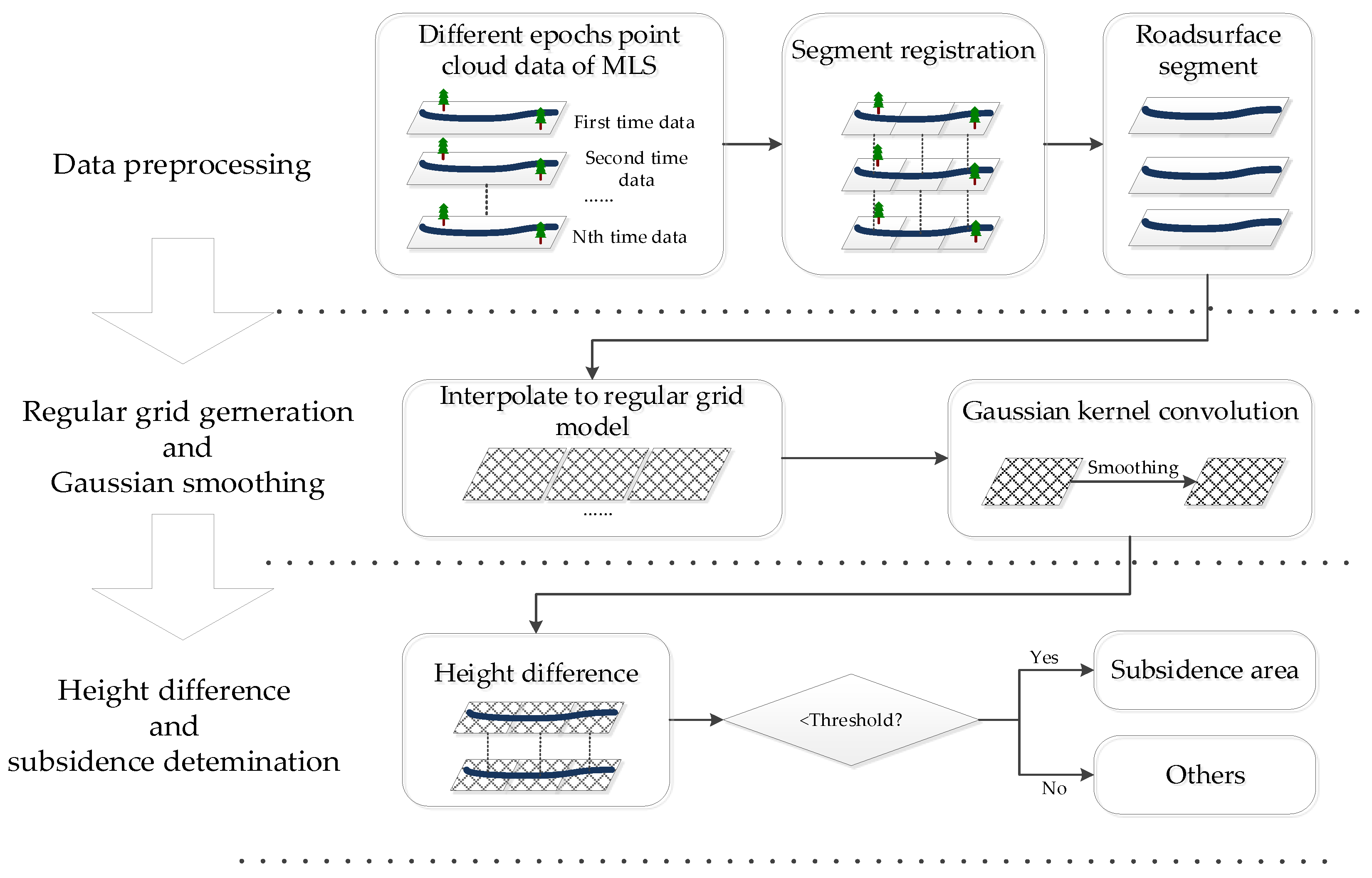
To distinguish the positive and negative results obtained by comparing data from different epochs, we used a model-to-model comparison method. The main steps in the method include data preprocessing for road surface points separation, regular grid square generation, smoothing using Gaussian kernel convolution, and a comparison for subsidence area determination. The workflow is shown in Figure 1.
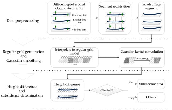
Figure 1.
Data processing workflow.
2.1. Data Preprocessing
Data preprocessing involves processing raw multitemporal point cloud data with the goal of obtaining pavement point cloud data that can be directly compared. This process mainly includes multitemporal data coregistration, the separation of ground points and nonground points in point cloud data, and pavement point extraction.
Data from different epochs need to be matched because of the positioning error associated with data acquisition at different times. There have been many studies of point cloud matching including the iterative closet point method [21,22], the normal distributions transform [23], and the coherent point drift [17]. An occupancy map-matching method is used to estimate the translation and rotation of the vehicle [24]. Not all matching methods are suitable for change detection applications. To avoid introducing errors in the matching process, a drifting matching method should not be used. However, the registration accuracy needs to be guaranteed because the result has a notable influence on the point cloud comparison. The coherent point drift method may adjust the point cloud data according to the two temporal phases of data during point cloud processing [17], which may alter the field of change; therefore, a rigid registration method should be selected to avoid additional errors caused by registration. Positioning errors accumulate as the vehicle moves during data collection. We took the approach of segmenting road sections and matching them separately to reduce this influence in the matching stage.
Ground point and nonground point separation is usually the first and key step in processing MLS data [25]. A variety of methods and algorithms has been developed for road surface detection and extraction using MLS data. Such methods are mainly categorized into two-dimensional (2D) feature image-based and 3D point-based methods [26,27,28,29] according to the different data formats used. Converting 3D MLS point clouds into 2D georeferenced feature images can decrease computational complexity in the stage of road surface extraction. By using existing computer vision and image processing methods, road boundaries and pavements can be efficiently detected and extracted [30]. Urban roads have structured edges, and the height difference between roads and road curbs is usually designed to be 10~25 cm. The pavement point cloud is separated from other points based on the height difference between the road surface and road curb [31].
2.2. Regular Square Mesh (RSM) Generation
Disordered point cloud in the format of (x, y, z) can be used to generate a regular square mesh if the size of the square and the interpolation method are sufficiently chosen. For the purpose of detecting the subsidence of urban roads and changes in the elevation direction, the points were projected onto the XOY plane, and the Z values were interpolated. The size of the grid was determined mainly based on the point spacing. The data obtained by an MLS are high-density data, and the distance between points varies with the frequency of scanning sensors and the movement speed of the carrier platform. Therefore, the distance between the scanned points increases with the scanning distance. The distance between points along adjacent scan lines varies with the vehicle movement speed. To obtain high-quality scan data, scan measurements are usually obtained at a fixed speed in the scan area, and the distance between scan lines is relatively stable. The typical distribution of points in the road area is smallest in the middle of the road (near the scanned lane), and spacing increases towards the edge of the road. Notably, high-density data are helpful for improving the accuracy of modeling [32]. When the size of a square is smaller than the minimum point spacing, the point cloud data can retain the full accuracy of the original data. However, for large amounts of point cloud data, the time cost for this process can be very large.
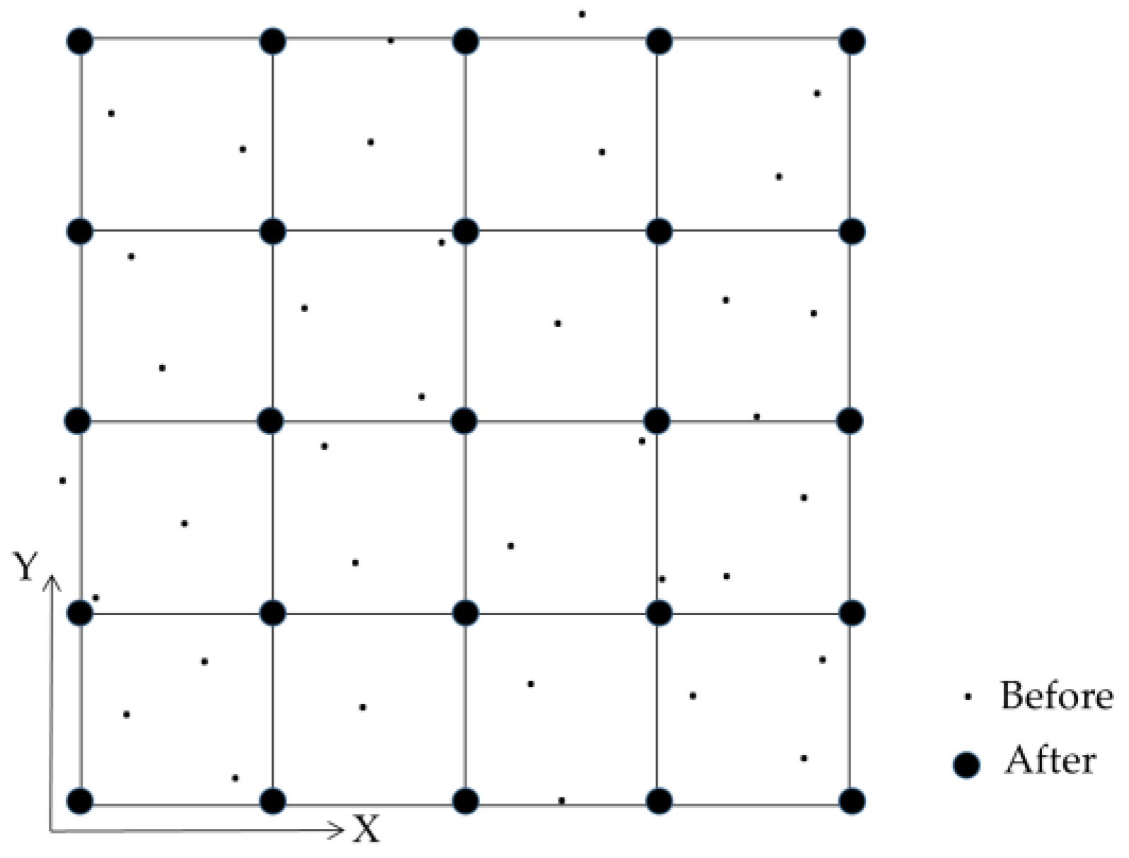
A suitable interpolation method can effectively preserve data accuracy, especially if the grid size is selected to be similar to the point spacing. Therefore, we used the nearest point interpolation method for modeling. Due to the large data volume of point cloud data, the nearest point difference method could effectively reduce the computing volume of interpolation. Since the grid size is close to the point spacing, this interpolation method can preserve data accuracy effectively as well. The specific implementation is to find the point nearest to a grid point to be inserted and to use the corresponding z value as the inserted value. In this process, if two or more points are determined to be nearest to each other, the average of the points is calculated and assigned to the interpolated point. Figure 2 shows the point distribution from a top view before and after the interpolation step.
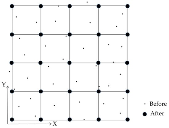
Figure 2.
Regular square mesh interpolation.
2.3. Smoothing Using Gaussian Kernel Convolution
The data acquisition principle for a point cloud is to obtain the distance and angle information of a target by recording the reflection signal of the target and then calculating the corresponding 3D coordinate information. In this process, there are various sources of errors [25,33]. Roads are considered to be artificial structures designed as flat or curved surfaces. When a mobile LiDAR system acquires data, due to error, the road point cloud is not in a flat or curved surface, and this variation is defined as roughness. Based on the high-frequency measurement speed of LiDAR and the slow change in road surface elevation, we performed Gaussian smoothing for the data to reduce the effect of high-frequency errors on the results.
The two-dimensional Gaussian function used to smooth the model was:
where w is the weight of point (x, y, z), ∆x and ∆y are the distances from the center point in the x direction and y direction, respectively, and σ is the standard deviation, which was used to determine the degree of smoothing. Convolution was applied to update the value of the central point by using the weighted average value of the data around the current point. In the data processing stage, z(x,y) for a given point was updated by convolving the z values of the surrounding points with the following Gaussian weight function:
where zg is the updated z value after Gaussian convolution and n is the number of points involved in calculations in one direction (x-axis direction or y-axis direction).
In this data processing, n and σ were determined and adjusted to the pavement roughness. To explore the impact of LiDAR errors on the parameters, we designed simulated experiments, in which only ranging errors existed, and the road pavement and subsidence were ideal. The gird size and n determine the actual Gaussian smoothing cell size jointly. The actual smoothing cell size can be adjusted by the pavement roughness [34]. When the road is determined to be good by pavement roughness [35], the smoothing unit can be set relatively big, which contributes to the elimination of ranging errors. When the road is determined to be bad, the smoothing unit should be adjusted to be small to leave the road trends. The correlation of parameters and their impact on the experimental results are elaborated in Section 4.3.
2.4. Subsidence Area Determination
After data interpolation and smoothing, the difference in height was calculated for subsidence area determination. Since data from different epochs had the same values of x and y, we could obtain the height difference in the surrounding area.
where is the height difference for the corresponding points, is the newly obtained value, and is the previously obtained value.
Subsidence is a negative change in height. Thus, < 0 can be used to identify areas of subsidence. However, due to data errors and actual field requirements, a threshold value () is usually set to compare changes for subsidence area determination. A histogram can be used to reflect the distribution of elevation differences, and we analyzed the histogram of height differences in this study. A normal distribution should be observed if there is no subsidence. If ∆zmax is the maximum height difference and ∆zmin is the minimum height difference, it is known that ∆zmin ≈ −∆zmax and the number of positive and negative signs of the difference is approximately equal under the condition that there is no change of pavement. However, with the subsidence of the pavement, there are more negative signs, and ∆zmin is less than −∆zmax. Therefore, the threshold ∆h was determined by the following formula:
The road surface was sorted into two categories based on a comparison: if ∆z < ∆h, the area was a subsidence area, and if ∆z ≥ ∆h, the area was a different type of area.
3. Materials and Experiments
To test the effectiveness of the method, both a set of simulated data including ideal road surface point clouds and a set of real road surface data were used to simulate subsidence in the experiment.
3.1. Simulated Data
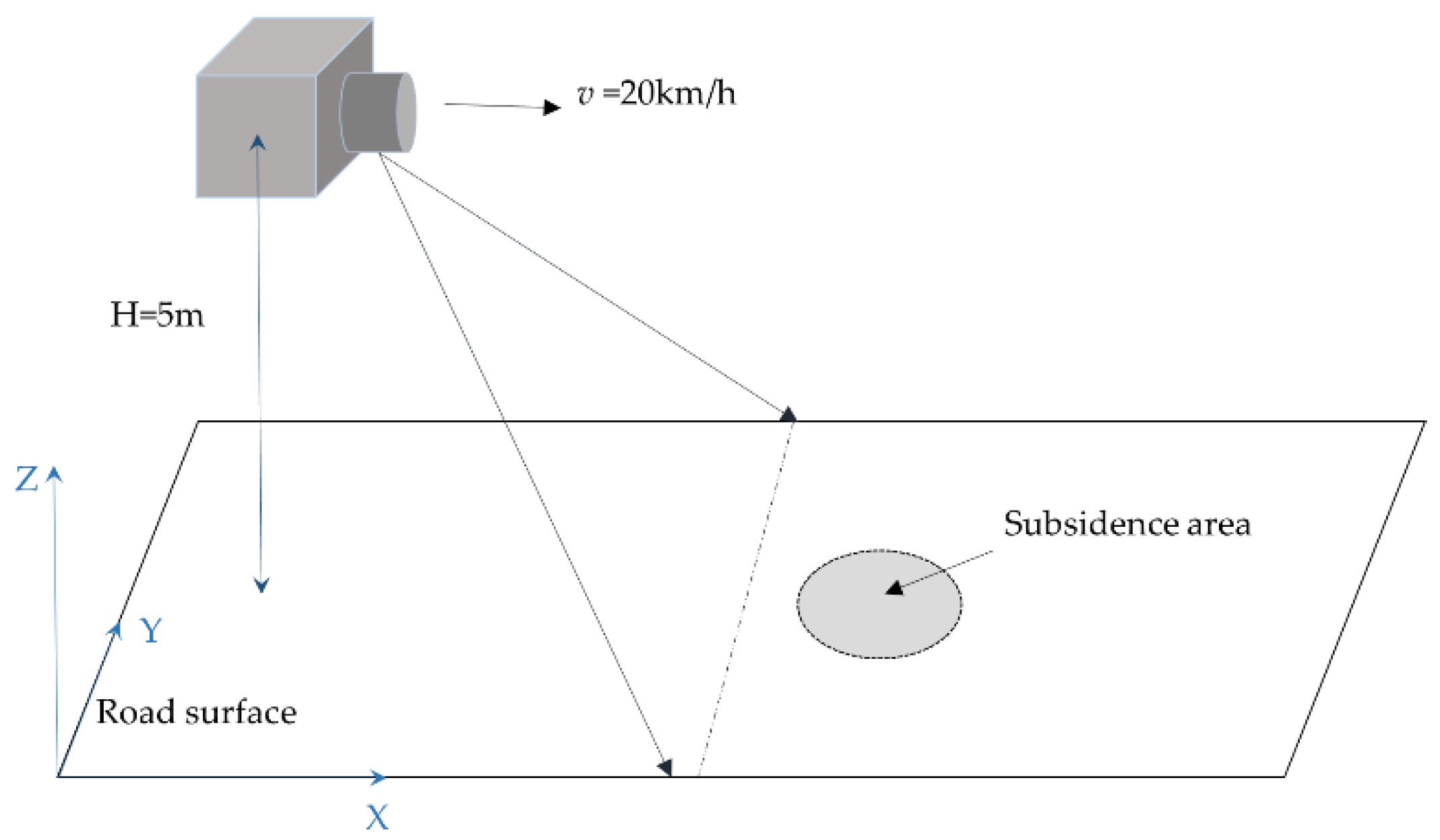
Figure 3 shows a diagram of simulation data acquisition. The data were generated by a self-developed software with a laser simulator in a point frequency of 300 MHz and a line frequency of 100 Hz. The laser scanning travel speed was 20.000 km/h. The simulated pavement length was 50 m (coordinates 100 to 150) and the width was 40 m (coordinates 80 to 120). The material of pavement was designed as an ideal reflection plane, expressed that the angular difference in laser incidence angle did not affect the point cloud data results. The height of the laser simulator from the pavement was 5 m. We defined x-positive as the direction of movement of the simulated sensor, y-positive as the leftward direction of sensor movement, and z-positive as the upward direction. The design positioning error was 0.05 m, and the scanning ranging error was 0.02 m. In the first simulation scan, the settlement area radius was not set, but in the second, third, and fourth scans, the radius of the circular settlement area was 3 m; additionally, settlement center values of 1 cm, 2 cm, and 4 cm, respectively, were used. The settlement value at distance d from the settlement center was :
where is the subsidence value at the center.
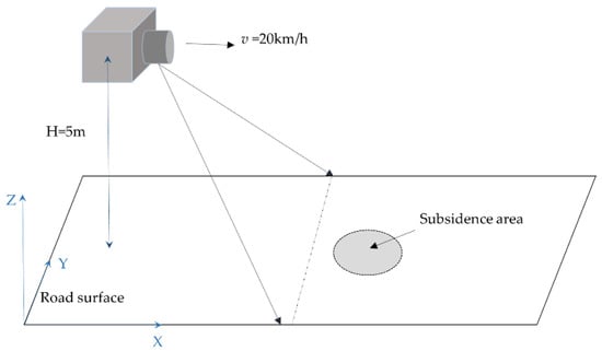
Figure 3.
Diagram of simulation data acquisition.
Thus, we acquired the simulated pavement data for five epochs shown in Table 1. The first pavement scan data were obtained for the original pavement without settlement. The second, third, fourth, and fifth pavement datasets were for circular settlement areas with central settlement values of 1 cm, 2 cm, 4 cm, and 8 cm, respectively.

Table 1.
Central settlement values of the simulated subsidence area.
Figure 4 shows the data obtained from the fourth payment simulation. Since there was no rotation or translation among data from different epochs, the preprocessing step could be omitted.
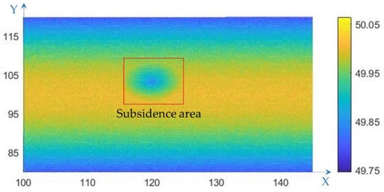
Figure 4.
Simulated road surface point cloud data (m).
3.1.1. Interpolation and Gaussian Convolution Smoothing Experiments
The laser simulator point frequency was 300 MHz, and the line frequency was 100 Hz. The laser scanning travel speed was 20.000 km/h. Accordingly, the point spacing for the same scan line ranged from 0.02 m to 0.05 m, and the distance between adjacent scan lines was 0.05 m on the pavement. A high density of data helped to improve the accuracy of the results. To balance the accuracy of the results and the computational burden, the grid size was set to 0.1 m. The result of interpolation for the fourth simulation is shown in Figure 5. With a positioning error of 0.05 m and scanning error of 0.02 m, the road surface was shown as a rough surface rather than a smooth plane.
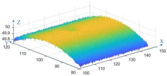
Figure 5.
Simulated road surface point cloud data (m).
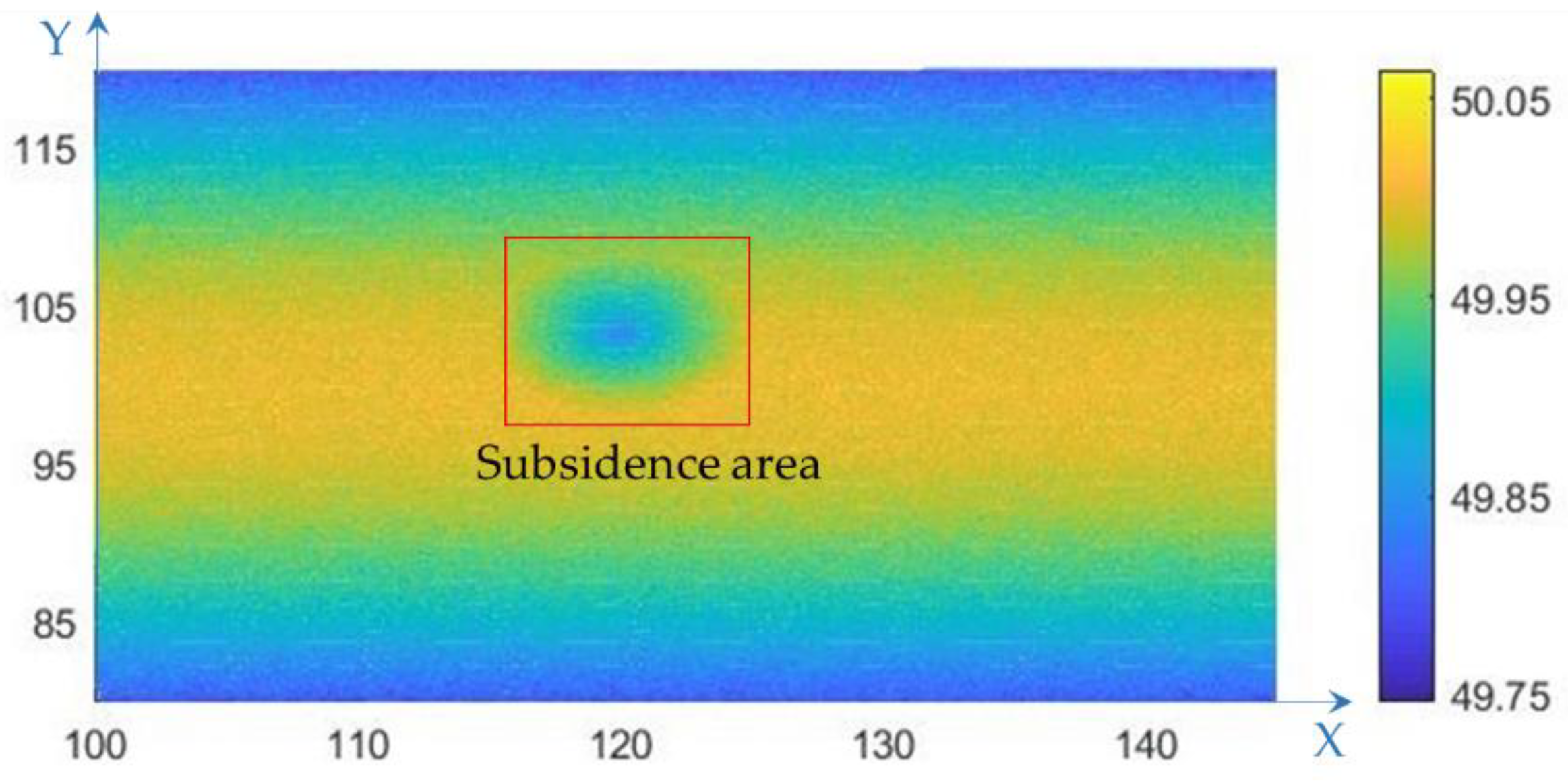
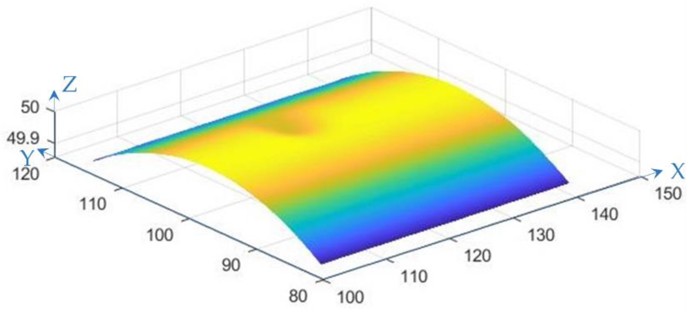
The smoothing was performed with MATLAB 2020. We smoothed the z-coordinate as a matrix with rows in x-direction and columns in y-direction. In the Gaussian kernel convolution process, the parameter was set to 10, and n was set to 61. The result of smoothing the 4 cm subsidence data is shown in Figure 6. After the smoothing process, the road surface was shown as a smooth surface, which was comparatively more similar to the real road pavement.

Figure 6.
Gaussian smoothing result for the simulated data (m).
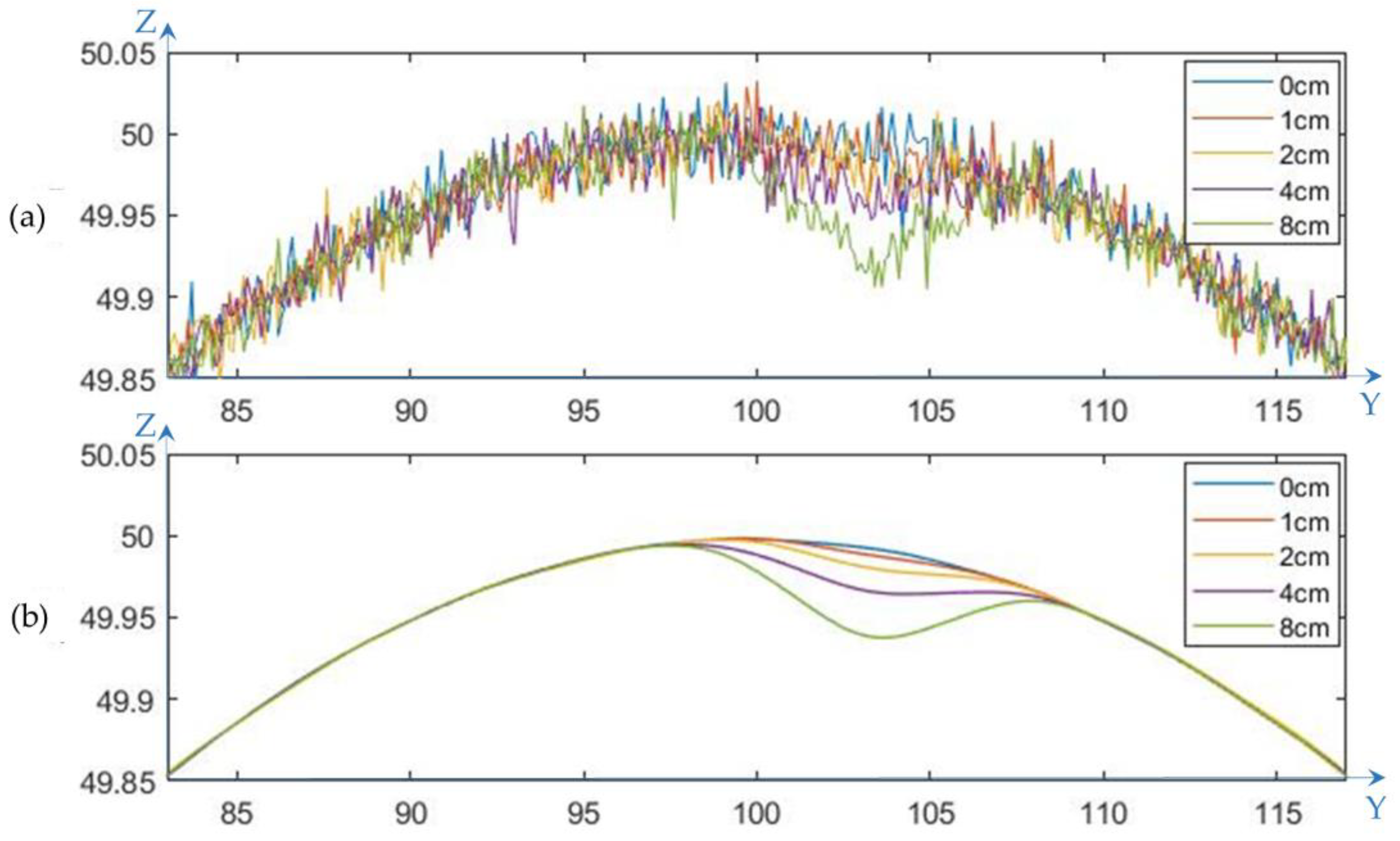
To clearly illustrate the data, a profile of all of the data is shown in Figure 7. Figure 7a is the result of interpolation, where the points were scattered around the road surface and the subsidence area was difficult to determine. Figure 7b shows the result after Gaussian smoothing; notably, the road surface profile better approximated the actual profile, and the subsidence area was easily identified by comparison.

Figure 7.
The profile obtained by simulating the subsidence center for all data (m): (a) interpolation result; (b) Gaussian smoothing result.
3.1.2. Height Difference Result
To validate the results for different settlement heights, we obtained four sets of height difference results by subtracting the first set of simulation data from the second, third, fourth, and fifth sets. Figure 8 is a section view of the results for the subsidence area. From the figure, the subsidence area could be easily distinguished from the unchanged area, where the values were approximately 0.
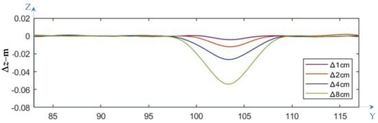
Figure 8.
Height difference results (profile through the subsidence center, m).
3.1.3. Subsidence Determination
While determining the subsidence area, a threshold was set to classify the subsidence area and the areas without subsidence. If the absolute value of the threshold was set too large, it would result in poor subsidence detection; in contrast, if it was set too small, subsidence areas would be introduced in error. To choose an appropriate threshold value, we analyzed the histograms of height differences. Figure 9 shows the histograms of height differences and the method used to determine the threshold.
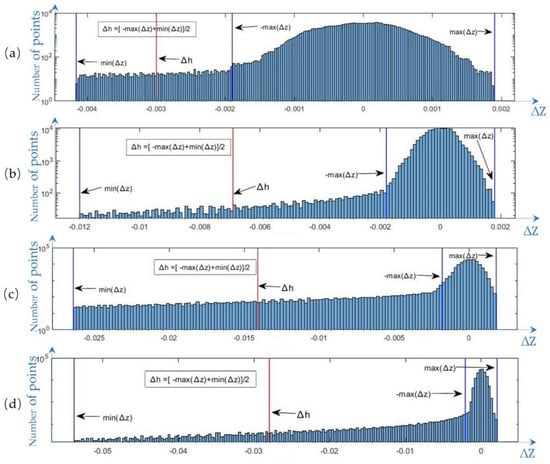
Figure 9.
Histograms of height differences (m): (a) 1 cm; (b) 2 cm; (c) 4 cm; (d) 8 cm.
As shown in Figure 8, the abscissa was the height difference , and the ordinate was the number of points. The subsidence area accounted for a small portion of the total road area. Therefore, the number of subsidence area points was very small in the histogram. To highlight the corresponding values, the ordinate was shown in the logarithmic form. In the figure, max () and min () were the maximum and minimum values of the height difference, respectively. The threshold value was set to the average of the sum of the negative max value and the minimum value:. Table 2 gives the threshold values for the different experimental datasets.
Table 2.
The threshold values for different subsidence datasets (cm).
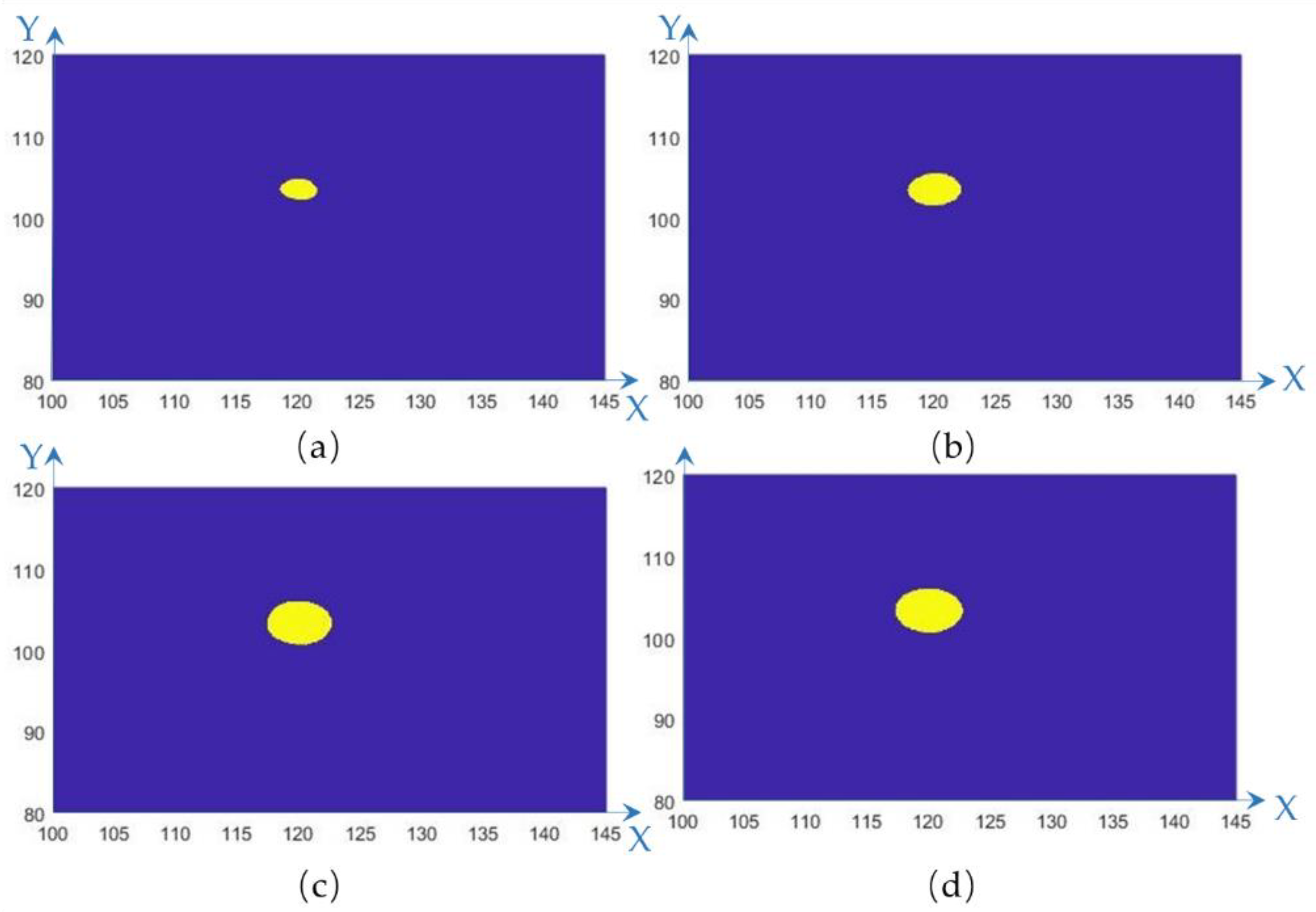
The subsidence region was determined through a comparison of simulated values and threshold values. The results were presented in a binary graph, with the yellow area representing the settled area and the blue background area representing the unsettled area, as shown in Figure 10. We could see that the settlement areas were accurately detected.
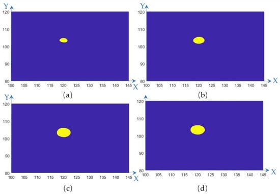
Figure 10.
Results of subsidence detection (m): (a) 1 cm; (b) 2 cm; (c) 4 cm; (d) 8 cm.
3.2. Real Data Experiments
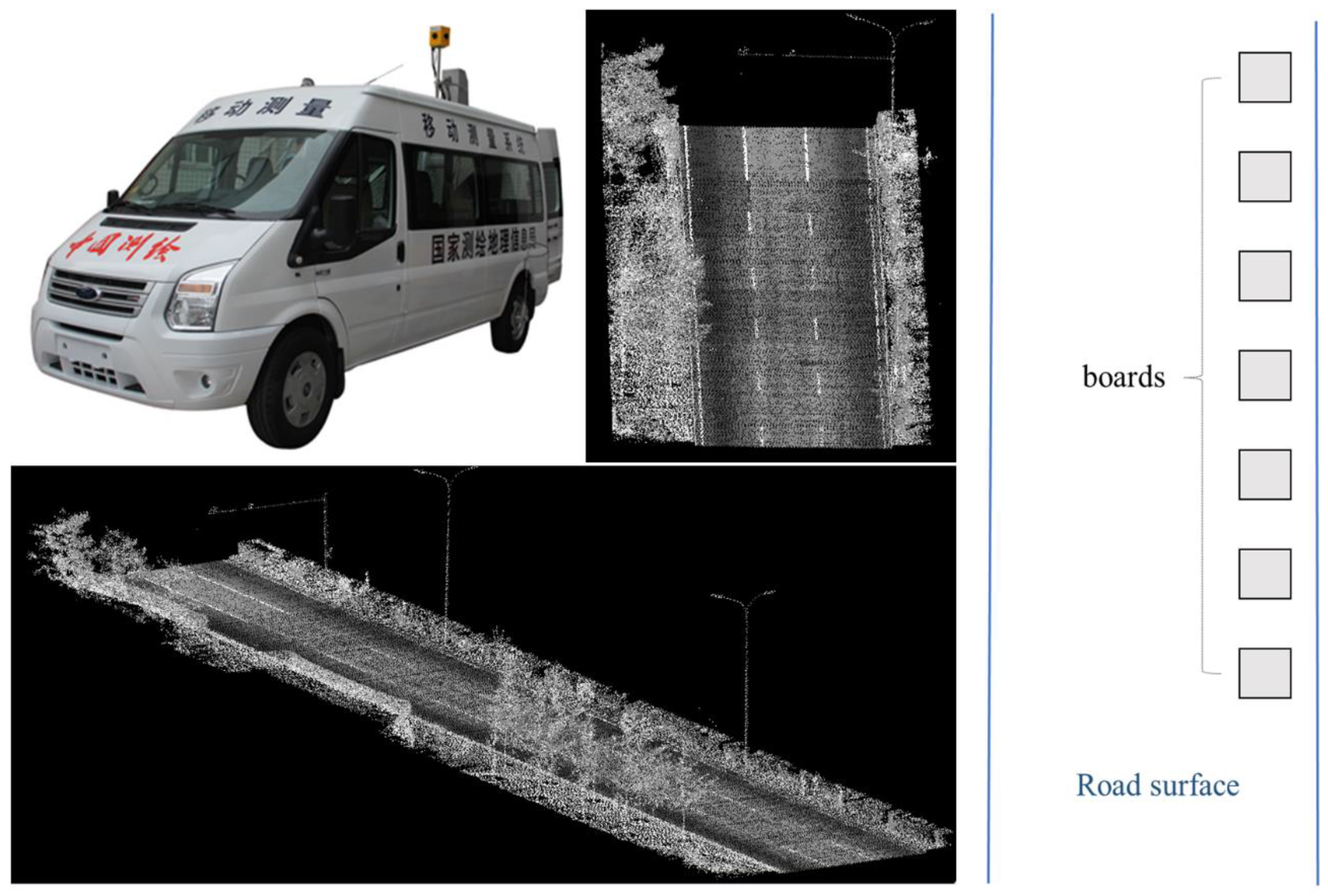
The real data were obtained with the SSW mobile measurement system (Figure 11), which integrated a laser scanner, an inertial measurement unit (IMU), a panoramic camera, an odometer, and a GPS antenna loaded on a transit vehicle. All the sensors were configured based on the relevant software and an embedded computer and synchronized with the GPS time. The x-direction of the acquired data was the right side of the vehicle movement direction, the y-direction was the vehicle movement direction, and z-direction was upward. The side spacing of points was 0.03 m~0.04 m on the road surface, and the line spacing was approximately 0.05 m. The obtained data accuracy was 10 mm. The study area was located in a section of Xiaotun Road, Fengtai District, Beijing, China. To simulate subsidence, seven boards were placed on the road. A height-adjustable nail was placed below the center of each board to control the amount of change in the center height. We collected pavement data with the nail height set at 15 mm, 10 mm, 5 mm, and 0 mm (without nail placement). The pavement data were obtained over approximately 90 m.
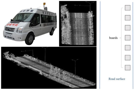
Figure 11.
The real experimental data and acquisition system.
3.2.1. Data Preprocessing: Registration and Pavement Point Segmentation
Data preprocessing mainly included registration and road surface segmentation. Since the road was a long narrow target, we divided the experimental road into three parts (each part was approximately 30 m long) and aligned them separately. The rigid ICP (iterative closest point) alignment method was used to avoid introducing additional errors in the registration stage. The initial positions of the two sets of point clouds were crucial for ensuring the accuracy of the matching results. The MLS included a positioning system so that the acquired data were spatial point cloud data in a geodetic coordinate system. Therefore, the data obtained by the MLS were approximately aligned in the same coordinate system. Using ground control points for rough alignment is a common method. Since the test system had already resolved the point cloud data to geodetic coordinates, and the process of accurate alignment had to be performed, we did not set ground control points for rough alignment. The ICP algorithm was used to implement an accurate matching process for the point cloud data, as described below.
Assume that p is the set of points to be aligned and Q is the set of target points. The main steps in registration are as follows:
- (1)
- Select points qi in the target point set Q (downsampling).
- (2)
- Find points pi in p to be aligned with the corresponding points qi in the point set Q such that ||pi − qi|| is minimized.
- (3)
- Calculate the rotation matrix R3×3 and translation matrix T3×1 from the coordinates of point pi to qi.
- (4)
- Using the rotation matrix R3×3 and translation matrix T3×1, update the point set p:
- (5)
- Calculate the average distance between pi′ and the corresponding point qi:
- (6)
- Judgment: If d is less than the given threshold or the number of loops is greater than the preset number, stop the calculation; otherwise, return to step 2 for looping until the convergence condition is satisfied.
To evaluate the effect of the matching process on the results, we analyzed the data in the elevation direction after the pavement gridding in Section 4.
Urban roads are manufactured infrastructure components with flat and smooth planes, and road edges usually have curbstones. The height difference between the road and road curbs is usually designed to be 10~25 cm, and this difference can be used for the separation of road surfaces and other points. Using this characteristic, we used the region-growing algorithm [36] based on the height difference and slope [37] limitations for roads to extract pavement points. The specific steps were as follows:
- Seed point selection. The key to the region growing method is the selection of seed points. Since urban pavement is continuous, pavement can be considered a plane. The accurate selection of one seed point for region growth is important in the judgement process. It is very common to select the lowest point or the point with the lowest curvature as the ground seed point [38]. However, if the lowest point is used, it must be verified that the lowest point is not a noise point, although the probability of such a situation is very low. Using the point with the lowest curvature as the seed point is a more robust method, but this method can result in a large computational cost due to the large amount of data required. In our experiment, we used the manual method to select the pavement seed points because it is the fastest and most accurate approach.
- Define the growth conditions. When a point meets the following conditions, it is determined to be a ground point.where Tdz is the height difference threshold and Tslope is the slope threshold. dz and slope are the elevation difference and slope values for the current seed point and its k-nearest neighbor point, respectively. The values of dz and slope were obtained from the following equations.
- Finish growing. The growth is finished when none of the ungrown neighboring points of the current point satisfy condition 2.
In the experiment, k was set to 8, which means that the 8 nearest points of the seed point were searched. To obtain better results, series of elevation and slope thresholds were tested. Figure 12 shows the results for Tdz = 0.015 m and Tslope = 30°. From the figure, we could see that the pavement points were effectively separated from other points, including plants and road curbs.
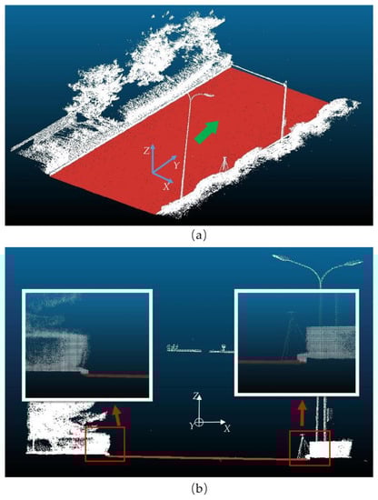
Figure 12.
Results of road surface segmentation: (a) 3D view; (b) close-up views of road edges projected in the XOZ plane.
3.2.2. Regular Grid Model and Gaussian Convolution Smoothing
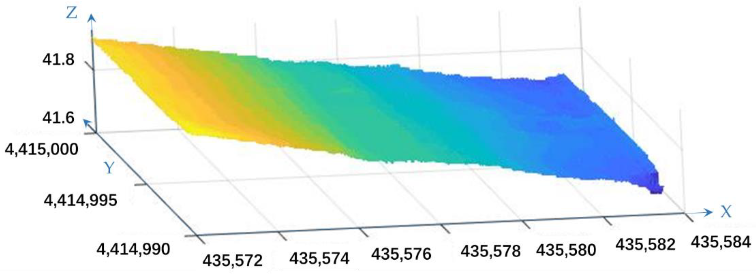
To balance accuracy and the computational time, we chose 0.05 m as the grid size. This value could preserve data accuracy and maximize the speed of computations. Figure 13 shows a portion of the road pavement interpolation results.

Figure 13.
A portion of road pavement interpolation results (m).
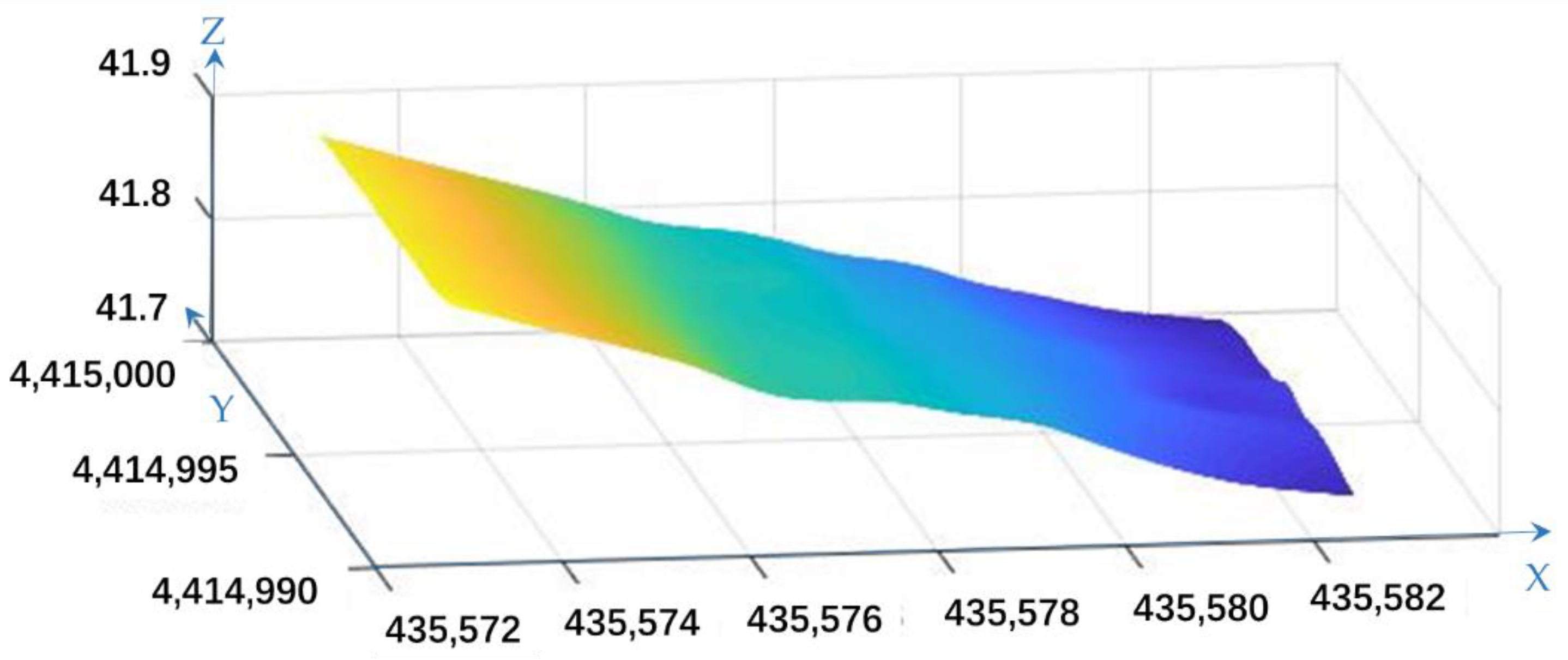
Two-dimensional Gaussian smoothing can be achieved by convolving with a two-dimensional smoothing unit in one step or by row convolution with a line Gaussian unit, followed by column convolution with a line Gaussian unit in two steps. During the experiments, the boards simulating subsidence were close to the edge of the road. To effectively preserve the boundary data, we used a two-step implementation to smooth the data: Gaussian smoothing in one direction followed by smoothing in the other vertical direction. The smoothing was performed with MATLAB 2020. We smoothed z-coordinate as a matrix with rows in x-direction and columns in y-direction. The Gaussian parameter was set to 10 and n was set to 51. The result obtained after Gaussian convolution smoothing is shown in Figure 14.

Figure 14.
A portion of the Gaussian smoothing results (m).
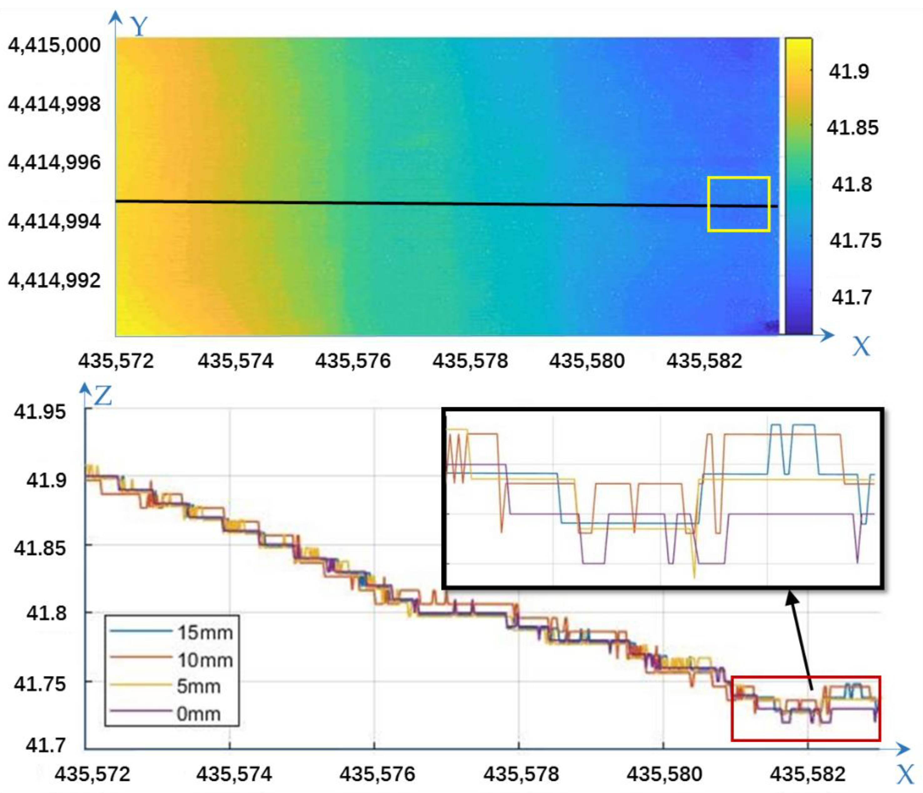
To clearly illustrate the data, the profile obtained by simulating the subsidence area was visualized. As shown in Figure 15 and Figure 16, the black line was the profile position, and the yellow frame was the position where the board was set. From the figures, the road surface was discontinuous in elevation before smoothing, and it was continuous and approximately accurate after smoothing. In the board area, the data seemed more accurate before smoothing, but the height difference between points and the board was not clear. After smoothing, the board edge was not distinguished, but the height difference was clear.
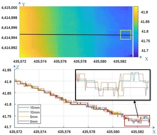
Figure 15.
The profiles for all sets of interpolation results (m).
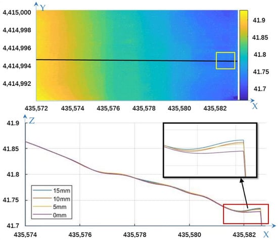
Figure 16.
The profiles for all sets of Gaussian smoothing results (m).
3.2.3. Height Difference Results
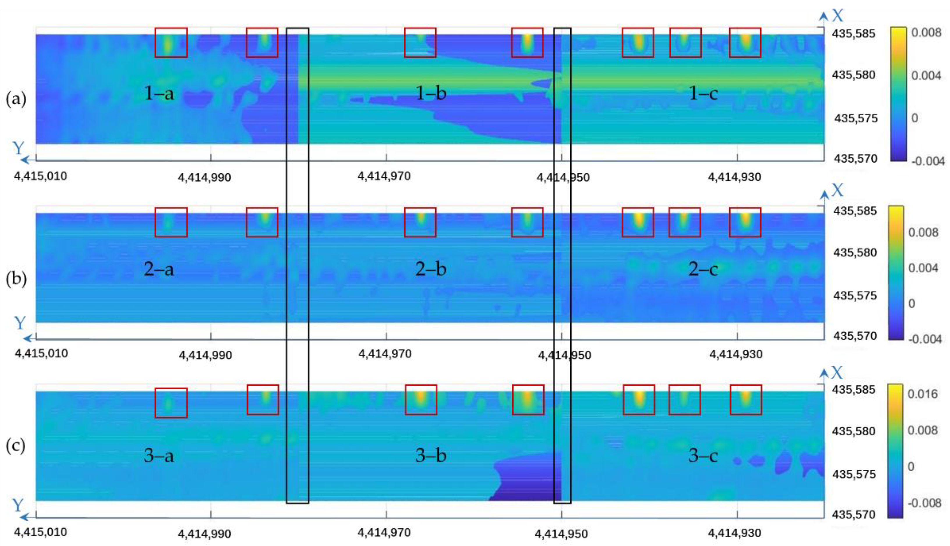
The experimental results are shown in Figure 17. Since the board was used to simulate the subsidence area, we used the data obtained without the board and subtracted the data obtained with the board to calculate the final values. In this way, three sets of data were acquired: 0–5 mm, 0–10 mm, and 0–15 mm sets. Figure 16 shows the negative differences. According to the different subsidence values, we divided the results into 1–, 2– and 3– periods of data, where 1– represents the results of 0–5 mm, 2– represents the results of 0–10 mm and 3– represents the results of 0–15 mm. According to the segmentation points of segment matching, the area of different time period data is divided into three parts: a, b and c. As shown in the figure, the area with a board could be distinguished (in the red frames). Since we split the data into three segments in the matching step, there was a gap (in the black frames) in the elevation of the segmented area in the result.
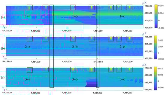
Figure 17.
Height difference results (negative, m): (a) 0–5 mm; (b) 0–10 mm; (c) 0–15 mm.
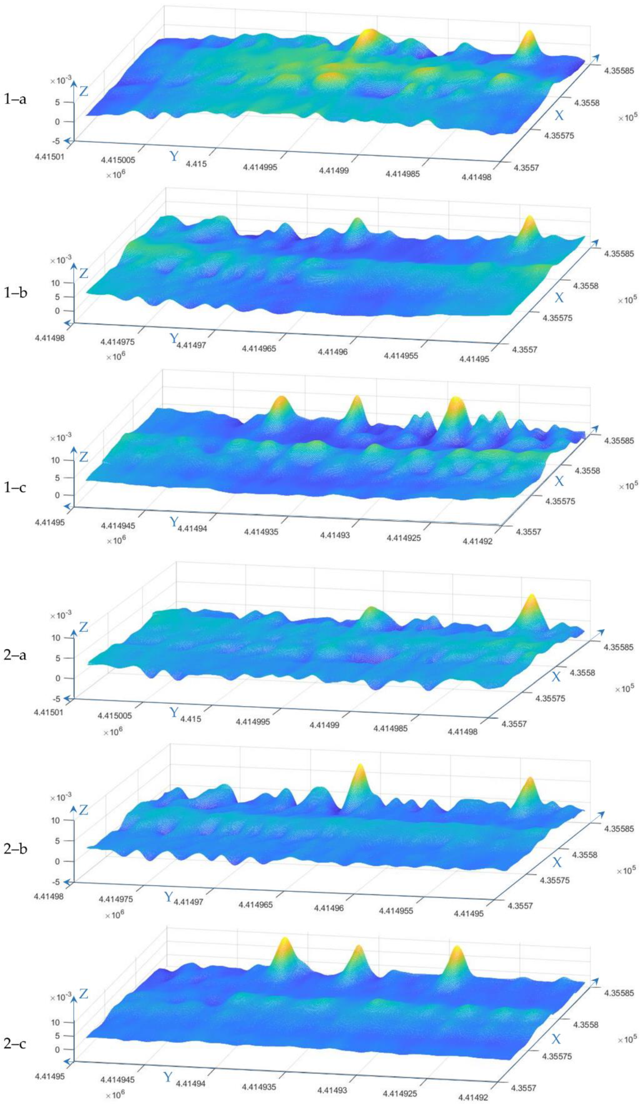
To provide a clear visualization of the results, Figure 18 shows three-dimensional views of the nine subregions in Figure 17.

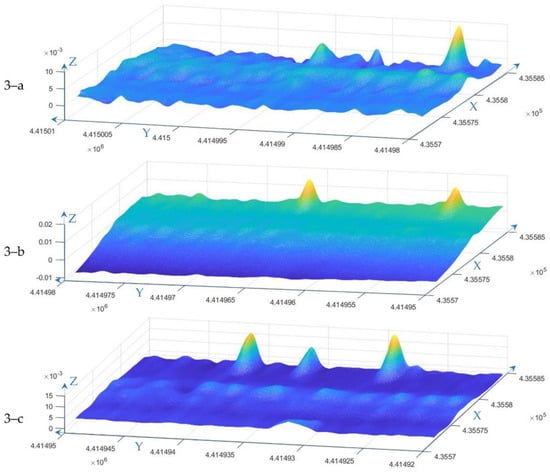
Figure 18.
Three-dimensional views of the subregions in Figure 17.
To show the results of the experiments comparing boards of different heights, Figure 19 shows the profiles of the board center. From the figure, the height difference where the board was placed (height change area) was lower than that in other areas. The areas with elevation change values of 0–5 mm, 0–10 mm, and 0–15 mm were also correctly represented. Moreover, the height difference exhibited regular fluctuations on one side of the road. The three blue lines marked the peaks of the 0–10 mm data, and the two other data classes exhibited similar trends.
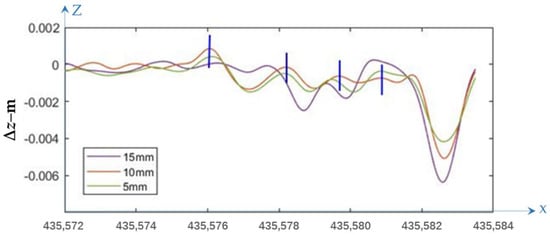
Figure 19.
Height difference results (profile through one board center, m).
3.2.4. Subsidence Detection
Since the road sections were matched segmentally, the matching parameters were different for each road section. Thus, the height difference between different road sections could also be different. To reduce the influence of the difference between road sections on threshold selection, it was necessary to select a threshold value for each road section to identify the pavement settlement area. The threshold values for each road segment are shown in Table 3.
Table 3.
Threshold values for each road segment (cm).
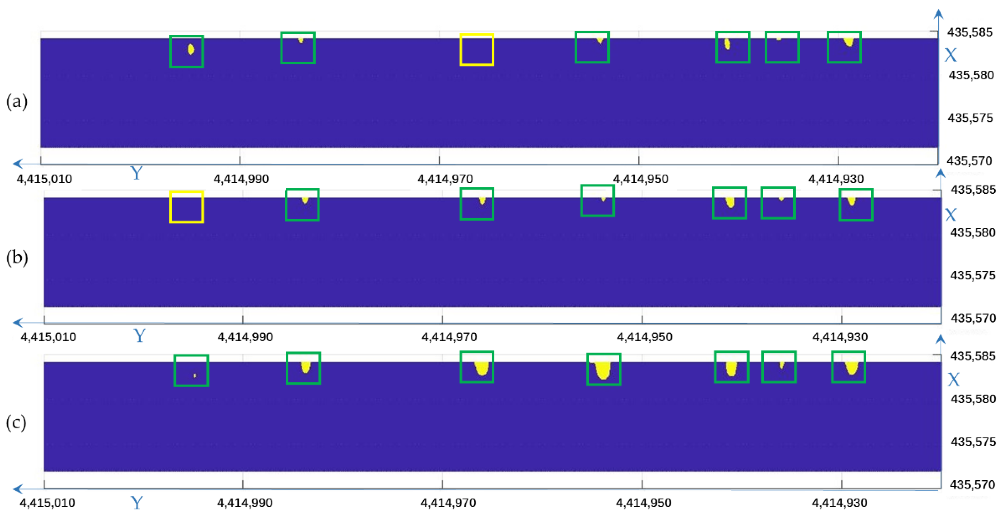
For comparison with the threshold value, the height difference results were converted into settlement detection values, as shown in Figure 20. The yellow areas were determined to be subsidence, the areas in the green frames denoted the board locations and the areas that were detected correctly, and the areas in the yellow frames denoted the board locations and the areas that were not detected. From the figure, there was one missing detection value in each of the 0–5 mm and 0–10 mm sets. There were no missing or incorrect values in the 0–15 mm set.
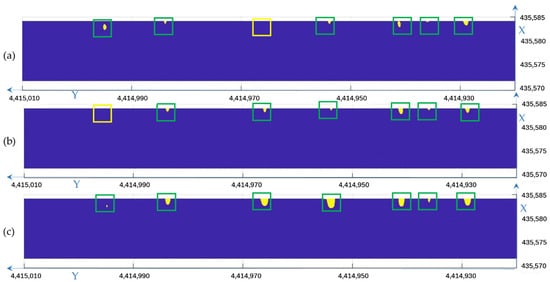
Figure 20.
Results of subsidence detection (m): (a) 0–5 mm; (b) 0–10 mm; (c) 0–15 mm.
4. Discussion
4.1. Simulated Data
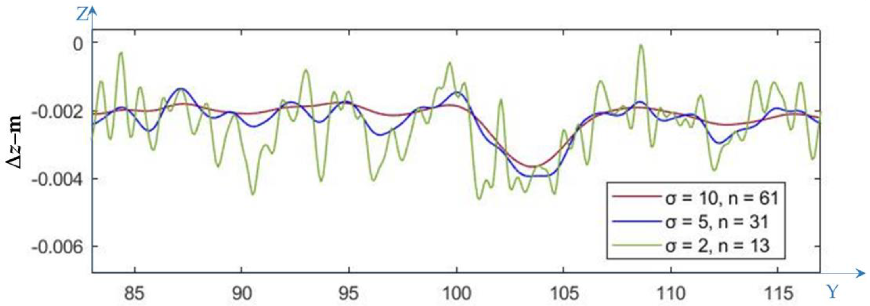
The method proposed in this paper performed well based on simulated data. The simulated data had a LiDAR localization error of 0.05 m and a ranging error of 0.02 m, and the combined error was 5.39 cm ( m). The proposed method could effectively reduce the systematic error in settlement detection. The experimental results indicated that the pavement settlement area was effectively detected. With the smoothing process in the proposed method, the test results at the true settlement values of 1 cm, 2 cm, 4 cm, and 8 cm were 0.41 cm, 1.21 cm, 2.64 cm, and 5.39 cm, respectively. To further analyze the influence of Gaussian parameters on the results, we tested different Gaussian kernel parameters. Due to the decreasing effect on the central grid with increasing distance and because the distance of the 3σ grid outside the central grid could be considered negligible, n was generally set to no more than 6σ + 1 to accelerate calculations. Figure 21 shows the results of 0–1 cm subsidence experiments, in which the parameters were set to (σ = 10, n = 61), (σ = 5, n = 31), and (σ = 2, n = 13). From the figure, we knew that the smoothing was effective for rough pavement points, and the larger σ was, the smoother the effect of the model was. However, this result came at the cost of undetectable areas of extremely small subsidence and the accuracy of detection in some subsidence areas.
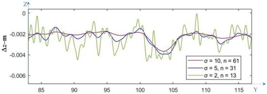
Figure 21.
Profile of smoothing results with different Gaussian parameters (m).
Since there was no rotation and translation among different periods of data, the simulated experiments could test the effect of smoothing on measurement results without matching errors. Furthermore, the simulated experiments provided a reference of the relationship between the parameters with the point spacing and settling area.
4.2. Real Data
In the experimental results based on the real data, the detection percentages for pavement settlement were 85.7%, 85.7%, and 100% for elevation changes of 5 mm, 10 mm, and 15 mm, respectively. There was one missing detection in each of the 0–5 mm and 0–10 mm datasets, and there were no missing or incorrect values in the 0–15 mm dataset. The results indicated that the proposed method could effectively detect subcentimeter-level pavement settlement with data accuracy at 10 mm. According to the distribution of settlement detection errors, we assumed that the point cloud alignment error [4] was the main cause of the detection errors. Thus, we evaluated the distribution of registration results in the elevation direction to determine the effect of the matching accuracy on the results. After regular square interpolation, each region was interpolated into 601 × 243 grids, resulting in 146,043 location points. Table 4 shows the normally distributed fitting parameters for the registered point cloud data for elevation differences. μ is the average and S is the standard deviation.
Table 4.
Normally distributed fitting parameters for the registered point cloud elevation difference.
From the table, we could see that the average values were all approximately 0 mm. The μ value for the 0–5 mm results for the third region was closest to 0 at 0.0008 mm. The worst μ result was for the 0–15 mm data in the second region, but the value was close to 0 at −0.0220 mm. The S values were all less than 4 mm. Compared to the subsidence value, the result for the 0–5 mm data in the first section was the worst, with a subsidence value of 3.6212 mm. When detecting 10 mm or 15 mm settlement, S values of 3 mm or 4 mm could be considered to have little effect on the results. From the above analysis, we found that the registration process achieved a good result. Additionally, the matching process did not affect the detection of settlement, except possibly for the 0–5 mm settlement detection.
4.3. Parameters
In the interpolation process, the size of the square (s) was an important factor affecting the results, which also influenced the setting of Gaussian parameters and the calculation speed. It was determined by the points density and spacing. If the size of the square grid was set much larger than the point spacing, the point cloud data would be downsampled, which would cause accuracy loss. From the perspective of data accuracy preservation, it was better for s to be as small as possible. However, if the grid size was set much smaller than the point spacing, the computation would increase. The parameters of the Gaussian convolution kernels σ and n, respectively, controlled the degree of smoothing and the number of points involved. We could calculate the actual smoothing area size (l × l) of the Gaussian convolutional kernel unit according to the grid size (s) and number of points (n × n):
To achieve a better smoothing effect, l was desired to be relatively big, for example, 1 m~3 m in our experiments. Paradoxically, s was taken to be as small as possible to ensure the data accuracy. Under such preconditions, n needed to be taken as a large value to achieve the purpose. According to the probability density function of the normal distribution, it is known that the probability sum of n taking values in (−3σ, 3σ) was 99.73%. It indicated that when n > 6σ + 1, it seemed that the number of points involved in the smoothing calculation increased, but the points substantially involved in the calculation were located in (−3σ, 3σ) with the contribution of 99.73%. With all the above assumptions satisfied, σ could be taken as large as possible, but this came at the cost of a significant increase in computation. Under the constraints of the data accuracy, smoothing effect, and calculation volume, we gave the following suggestions for the values of the parameters. We tested the impact of different grid sizes on the results and recommended that a fine result could be obtained when the grid size was set to no more than five times the point average spacing. In our experiment, the simulated data point spacing was 0.02 m~0.05 m (point average spacing was 0.035 m). Due to the data volume, we chose 0.1 m as the grid size. The real data point spacing was 0.03 m~0.05 m (point average spacing 0.04 m), and we chose 0.05 m as the grid size in order to keep the data accuracy.
4.4. Others
We validated the proposed method using simulated data and real pavement data, but strictly speaking, the settlement areas in our real data were also simulated. It is a more convincing validation on real cases of subsidence data, which is also our next work. The comparison with other methods was still lacking, but in the process of experimental comparison, we compared the results before and after smoothing to illustrate the positive effect of smoothing on point cloud comparison. It was considered that the comparison results before smoothing were general point cloud processing results, while the results after smoothing illustrated the effectiveness of our proposed method.
The purpose of Gaussian convolution processing is to reduce the error-detected subsidence areas by smoothing the pavement. However, the subsidence area would be smoothed as well. Therefore, the precision of settlement values was also reduced. The proposed method aimed to achieve a fast localization of subsidence areas. If the value of the subsidence area needs to be correctly detected, the method may not be appropriate. A possible solution is to first use the method proposed in this paper to locate the area and then use the GNSS or TLS to obtain the values in the located subsidence zone. For areas where subsidence areas perform abnormally, GPR (ground-penetrating radar) technology can be used to find the specific cause of subsidence from the perspective of the physical structure of the underground strata.
5. Conclusions
This study focused on urban road subsidence detection using point cloud data from an MLS system. A method that uses Gaussian kernel convolution to process regular grid data generated from point cloud data was proposed, and a histogram method was used to determine the appropriate thresholds. Simulated road data and real road data were tested, and the results were presented in the form of binary diagrams, which indicated that the detection effect was more accurate than that obtained by directly comparing meshes generated from point data. The conclusions were as follows:
First, smoothing high-density point cloud data could improve the accuracy of point cloud comparisons. The road surface could be considered as a smooth surface, while in high-density point clouds appeared as a rough plane, causing errors in the point cloud comparison. With the process of smoothing, the comparison errors could be effectively reduced.
Second, the method could detect the subsidence area, which was slightly lower than the accuracy of data acquisition. Theoretically, regions with subsidence values smaller than the accuracy of data acquisition were not detectable. With the proposed method, they were effectively detected. In the experiments, the subsidence values of 1 cm, 2 cm, and 4 cm, which were smaller than the data accuracy of 5.39 cm, were detected in simulated data and a subsidence value of 5 mm, which was smaller than the data accuracy of 10 mm, which was detected in real data.
Third, the method could effectively reduce the false detection probability. It was easy to determine a number of unsettled areas as settling areas using the threshold method. Using the method proposed for smoothing the data, the false detection rate could be effectively reduced. In terms of microsettlement detection, the reduction in the false detection rate had great practical significance for the detection results.
Finally, appropriate parameters, according to the pavement roughness, could achieve good experimental results. It was crucial to obtain promising results that chose an appropriate grid size and parameters of the Gaussian convolution kernel according to the smoothness of the pavement. If the pavement and the settlement area were gently sloping, the grid size and σ, and the corresponding n, could be adjusted to be appropriately larger to obtain better results. While, in this case, the pavement was not gently sloping or preferred to retain the pavement height variation trend, the grid size should have been adjusted to be appropriately smaller; thus, decreasing the values of σ and n and obtaining smaller areas of the settlement region. According to Equation (10), l could be determined by the per-known pavement roughness; then, the grid size and Gaussian parameters should have been adjusted according to l. l could be used as a sensitivity indicator for the subsidence area size. In other words, the method was most sensitive to the subsidence area of size l. Our next work should focus on quantitative effects of Gaussian smoothing parameters on pavement settlement detection, how the pavement roughness relates to the data accuracy, and quantitative effects on elevation.
Author Contributions
Conceptualization and resources, J.Z. (Jixian Zhang) and J.Z. (Jianzhang Zuo); methodology and investigation, H.S.; validation, H.S. and J.Z. (Jianzhang Zuo); data curation and writing—original draft preparation, H.S. and J.G.; writing—review and editing, X.L. and W.H.; supervision, J.G.; project administration, J.Z. (Jixian Zhang); funding acquisition, J.Z. (Jixian Zhang) and W.H. All authors have read and agreed to the published version of the manuscript.
Funding
This research was funded by the National Natural Science Foundation of China, grant number 41671440, the program of Ministry of Natural Resources of China, grant number 121134000000180009, and the National Key Research Development Program of China, grant number 2018YFF0215302.
Acknowledgments
We acknowledge researcher Xiangguo Lin of the Chinese Academy of Surveying and Mapping for his advice on the article.
Conflicts of Interest
The authors declare no conflict of interest.
References
- Baer, G.; Magen, Y.; Nof, R.N.; Raz, E.; Lyakhovsky, V.; Shalev, E. InSAR Measurements and Viscoelastic Modeling of Sinkhole Precursory Subsidence: Implications for Sinkhole Formation, Early Warning, and Sediment Properties. J. Geophys. Res. Earth Surf. 2018, 123, 678–693. [Google Scholar] [CrossRef]
- Yang, Y.; Zheng, Y.; Yu, W.; Chen, W.; Weng, D. Deformation monitoring using GNSS-R technology. Adv. Space Res. 2019, 63, 3303–3314. [Google Scholar] [CrossRef]
- Rius, A.; Nogués-Correig, O.; Ribó, S.; Cardellach, E.; Oliveras, S.; Valencia, E.; Park, H.; Tarongí, J.M.; Camps, A.; van der Marel, H.; et al. Altimetry with GNSS-R interferometry: First proof of concept experiment. GPS Solut. 2011, 16, 231–241. [Google Scholar] [CrossRef]
- Orellana, F.; Delgado Blasco, J.M.; Foumelis, M.; D’Aranno, P.J.V.; Marsella, M.A.; Di Mascio, P. DInSAR for Road Infrastructure Monitoring: Case Study Highway Network of Rome Metropolitan (Italy). Remote Sens. 2020, 12, 3697. [Google Scholar] [CrossRef]
- Chen, Y.; Yu, S.; Tao, Q.; Liu, G.; Wang, L.; Wang, F. Accuracy Verification and Correction of D-InSAR and SBAS-InSAR in Monitoring Mining Surface Subsidence. Remote Sens. 2021, 13, 4365. [Google Scholar] [CrossRef]
- Wang, L.; Deng, K.; Zheng, M. Research on ground deformation monitoring method in mining areas using the probability integral model fusion D-InSAR, sub-band InSAR and offset-tracking. Int. J. Appl. Earth Obs. Geoinf. 2020, 85, 101981. [Google Scholar] [CrossRef]
- Zhao, L.; Chen, B.; Liu, G.; WU, Y.; ZHou, Y.; Yang, Y.; Guo, T.; Han, D. Automatic Extrction and Analysis of Expressway Subsidence Based on Ground 3D Laser Scanning. J. Chongqing Jiaotong Univ. 2020, 39, 14–19. [Google Scholar]
- Anders, K.; Marx, S.; Boike, J.; Herfort, B.; Wilcox, E.J.; Langer, M.; Marsh, P.; Höfle, B. Multitemporal terrestrial laser scanning point clouds for thaw subsidence observation at Arctic permafrost monitoring sites. Earth Surf. Processes Landf. 2020, 45, 1589–1600. [Google Scholar] [CrossRef]
- Shen, Y.; Lindenbergh, R.; Wang, J. Change Analysis in Structural Laser Scanning Point Clouds: The Baseline Method. Sensors 2017, 17, 26. [Google Scholar] [CrossRef] [Green Version]
- Zhang, D.; Zou, Q.; Lin, H.; Xu, X.; He, L.; Gui, R.; Li, Q. Automatic pavement defect detection using 3D laser profiling technology. Autom. Constr. 2018, 96, 350–365. [Google Scholar] [CrossRef]
- Antova, G. Application of areal change detection methods using point clouds data. IOP Conf. Ser. Earth Environ. Sci. 2019, 221, 12082. [Google Scholar] [CrossRef]
- Lindenbergh, R.; Pietrzyk, P. Change detection and deformation analysis using static and mobile laser scanning. Appl. Geomat. 2015, 7, 65–74. [Google Scholar] [CrossRef]
- Heinz, E.; Eling, C.; Klingbeil, L.; Kuhlmann, H. On the applicability of a scan-based mobile mapping system for monitoring the planarity and subsidence of road surfaces—Pilot study on the A44n motorway in Germany. J. Appl. Geod. 2020, 14, 39–54. [Google Scholar] [CrossRef]
- Fuse, T.; Yokozawa, N. Development of a Change Detection Method with Low-Performance Point Cloud Data for Updating Three-Dimensional Road Maps. ISPRS Int. J. Geo-Inf. 2017, 6, 398. [Google Scholar] [CrossRef] [Green Version]
- Xiao, W.; Vallet, B.; Bredif, M.; Paparoditis, N. Street environment change detection from mobile laser scanning point clouds. ISPRS J. Photogramm. Remote Sens. 2015, 107, 38–49. [Google Scholar] [CrossRef]
- Barnhart, T.; Crosby, B. Comparing Two Methods of Surface Change Detection on an Evolving Thermokarst Using High-Temporal-Frequency Terrestrial Laser Scanning, Selawik River, Alaska. Remote Sens. 2013, 5, 2813–2837. [Google Scholar] [CrossRef] [Green Version]
- Andriy, M. Point set registration: Coherent point drift. IEEE Trans. Pattern Anal. Mach. Intell. 2010, 12, 2262–2275. [Google Scholar]
- Hao, X.; Liang, C.; Manchun, L.; Yanming, C.; Lishan, Z. Using Octrees to Detect Changes to Buildings and Trees in the Urban Environment from Airborne LiDAR Data. Remote Sens. 2015, 7, 9682–9704. [Google Scholar]
- Richter, R.; Kyprianidis, J.E.; Döllner, J. Out-of-Core GPU-based Change Detection in Massive 3D Point Clouds. Trans. GIS 2013, 17, 724–741. [Google Scholar] [CrossRef]
- Lercari, N. Monitoring earthen archaeological heritage using multi-temporal terrestrial laser scanning and surface change detection. J. Cult. Herit. 2019, 39, 152–165. [Google Scholar] [CrossRef] [Green Version]
- Zhang, Z. Iterative point matching for registration of free-form curves and surfaces. Int. J. Comput. Vis. 1994, 13, 119–152. [Google Scholar] [CrossRef]
- Besl, P.J.; Mckay, H.D. A method for registration of 3-D shapes. IEEE Trans. Pattern Anal. Mach. Intell. 1992, 14, 239–256. [Google Scholar] [CrossRef]
- Biber, P. The normal distributions transform: A new approach to laser scan matching. In Proceedings of the 2003 IEEVRSJ InU Conference on Intelligent Robots and Systems, Las Vegas, NV, USA, 27 October–1 November 2003. [Google Scholar]
- Dimitrievski, M.; Hamme, D.V.; Veelaert, P.; Philips, W. Robust Matching of Occupancy Maps for Odometry in Autonomous Vehicles. In Proceedings of the International Conference on Computer Vision Theory & Applications, Rome, Italy, 27–29 February 2016. [Google Scholar]
- Ma, L.; Li, Y.; Li, J.; Wang, C.; Wang, R.; Chapman, M. Mobile Laser Scanned Point-Clouds for Road Object Detection and Extraction: A Review. Remote Sens. 2018, 10, 1531. [Google Scholar] [CrossRef] [Green Version]
- Kumar, P.; Lewis, P.; McElhinney, C.P.; Boguslawski, P.; McCarthy, T. Snake Energy Analysis and Result Validation for a Mobile Laser Scanning Data-Based Automated Road Edge Extraction Algorithm. IEEE J. Sel. Top. Appl. Earth Obs. Remote Sens. 2017, 10, 763–773. [Google Scholar] [CrossRef]
- Guan, H.; Li, J.; Yu, Y.; Cheng, W.; Chapman, M.; Yang, B. Using mobile laser scanning data for automated extraction of road markings. ISPRS J. Photogramm. Remote Sens. 2014, 87, 93–107. [Google Scholar] [CrossRef]
- Yan, L.; Liu, H.; Tan, J.; Li, Z.; Xie, H.; Chen, C. Scan Line Based Road Marking Extraction from Mobile LiDAR Point Clouds. Sensors 2016, 16, 903. [Google Scholar] [CrossRef]
- Ye, C.; Li, J.; Jiang, H.; Zhao, H.; Ma, L.; Chapman, M. Semi-Automated Generation of Road Transition Lines Using Mobile Laser Scanning Data. IEEE Trans. Intell. Transp. Syst. 2020, 21, 1877–1890. [Google Scholar] [CrossRef]
- Serna, A.; Marcotegui, B.; Hernández, J. Segmentation of Façades from Urban 3D Point Clouds Using Geometrical and Morphological Attribute-Based Operators. ISPRS Int. J. Geo-Inf. 2016, 5, 6. [Google Scholar] [CrossRef]
- Guan, H.; Li, J.; Yu, Y.; Chapman, M.; Wang, C. Automated Road Information Extraction From Mobile Laser Scanning Data. IEEE Trans. Intell. Transp. Syst. 2015, 16, 194–205. [Google Scholar] [CrossRef]
- Abellán, A.; Jaboyedoff, M.; Oppikofer, T.; Vilaplana, J.M. Detection of millimetric deformation using a terrestrial laser scanner: Experiment and application to a rockfall event. Nat. Hazards Earth Syst. Sci. 2009, 9, 365–372. [Google Scholar] [CrossRef] [Green Version]
- Guan, H.; Li, J.; Cao, S.; Yu, Y. Use of mobile LiDAR in road information inventory: A review. Int. J. Image Data Fusion 2016, 7, 219–242. [Google Scholar] [CrossRef]
- Alhasan, A.; White, D.J.; De Brabanter, K. Spatial pavement roughness from stationary laser scanning. Int. J. Pavement Eng. 2017, 18, 83–96. [Google Scholar] [CrossRef]
- Meyer, F.J.; Ajadi, O.A.; Hoppe, E.J. Studying the Applicability of X-Band SAR Data to the Network-Scale Mapping of Pavement Roughness on US Roads. Remote Sens. 2020, 12, 1507. [Google Scholar] [CrossRef]
- Zhang, W.; Zhou, F.; Wang, L.; Sun, P. Region Growing Based on 2-D–3-D Mutual Projections for Visible Point Cloud Segmentation. IEEE Trans. Instrum. Meas. 2021, 70, 1–13. [Google Scholar] [CrossRef]
- Axelsson, P. DEM Gerneration from Laser Scanner Data Using Adaptive TIN Models. Int. Arch. Photogramm. Remote Sens. 2000, 33, 110–117. [Google Scholar]
- Khaloo, A.; Lattanzi, D. Robust normal estimation and region growing segmentation of infrastructure 3D point cloud models. Adv. Eng. Inform. 2017, 34, 1–16. [Google Scholar] [CrossRef]


Publisher’s Note: MDPI stays neutral with regard to jurisdictional claims in published maps and institutional affiliations. |
© 2022 by the authors. Licensee MDPI, Basel, Switzerland. This article is an open access article distributed under the terms and conditions of the Creative Commons Attribution (CC BY) license (https://creativecommons.org/licenses/by/4.0/).