A Landslide Numerical Factor Derived from CHIRPS for Shallow Rainfall Triggered Landslides in Colombia

Abstract

Despite great advances in remote sensing technologies, accurate satellite information is sometimes challenged in tropical regions where dense vegetation prevents the instruments from retrieving reliable readings. In this work, we introduce a satellite-based landslide rainfall threshold for the country of Colombia by studying 4 years of rainfall measurements from The Climate Hazards Group Infrared Precipitation with Stations (CHIRPS) for 346 rainfall-triggered landslide events (the dataset). We isolate the two successive rainy/dry periods leading to each landslide to create variables that simulate the dynamics of antecedent wetness and dryness. We test the performance of the derived variables (Rainfall Period 1 (PR1), Rainfall Sum 1 (RS1), Rainfall Period 2 (PR2), Rainfall Sum 2 (RS2), and Dry Period (DT)) in a logistic regression that includes three (3) static parameters (Soil Type (ST), Landcover (LC), and Slope angle). Results from the logistic model describe the influence of each variable in landslide occurrence with an accuracy of 73%. Subsequently, we use these dynamic variables to model a landslide threshold that, in the absence of satellite antecedent soil moisture data, helps describe the interactions between the dynamic variables and the slope angle. We name it the Landslide Triggering Factor—LTF. Subsequently, with a training dataset (65%) and one for testing (35%) we evaluate the LTF threshold performance and compare it to the well-known event duration (E-D) threshold. Results demonstrate that The LTF performs better than the E-D threshold for the training and testing datasets at 71% and 81% respectively.

1. Introduction

Landslides are a physical hazard that frequently result in devastating human and economic losses around the world [1,2,3]. There are various underlying geological, lithological, and morphological characteristics that make an area prone to these hazards. Nonetheless, landslides can happen as a result of anthropogenic activities or can be triggered by natural forces such as earthquakes, melting snow, or extreme precipitation [4,5,6].

Landslides that are triggered by rainfall are common phenomena in mountainous tropical regions. These landslides are associated with long-term, high-intensity periods of precipitation that have dangerous potential to initiate mass soil movement due to changes in pore pressure and seepage forces in the soil [7,8,9]. Rainfall-triggered landslides are usually shallow (0.3–2 m) and often driven by two different mechanisms. In the first, the hydraulic conductivity of the weathering profile decreases, creating a perched water flow that is parallel to the slope. This results in a reduction of the shear strength of the soil, which leads to slope failure. In the second mechanism, water from the surface advances on the slope while it is still unsaturated and, in this case, low suction results in a rigid mass slope failure [8,10].

Over the years, scholars have tried to define statistical or empirical correlations between slope failures and rainfall intensity and duration. These relationships are often defined mathematically as rain thresholds that attempt to define the rainfall curve in between the slope’s stability and failure zones [11]. Since their inception in Cane (1980) [12], precipitation thresholds have been established for Rainfall Intensity-Duration (I-D), Cumulative Rainfall Event-Duration (E-D), Cumulative Rainfall Event Intensity (E-I), Rainfall Cumulative (R), and other relationships between intraday rain and antecedent rainfall [13].

Inevitably, these thresholds are highly influenced by temporal and spatial factors such as the location, range of the study area, and the instruments (rain gauges or remote sensors) used to calculate them. To a large extent, in-situ sensors (gauges) have been used to derive rainfall thresholds in various areas of the world. In Indian’s Himalayan region, for example, several authors have used in-situ-based data for the definition of rainfall thresholds. These scholars combined intensity-duration thresholds based on the daily rainfall and antecedent rain by aggregating several days in different combinations, such as 2, 3, 5, and 20 days [14,15,16].

Nonetheless, recent advancements in satellite technologies have been a promising and reliable source of data to map and model susceptibility, hazard, risk, and landslide impacts in various areas of the world. Satellite products such as the Global Precipitation Measurement Mission (GPM), for example, provide rainfall estimates that can help evaluate rain as a landslide trigger at large scales [9,17]. Satellite soil moisture products have also been successfully adapted in various shallow landslide studies. Ray et al. (2007), for example, used moisture settings from the Advanced Microwave Scanning Radiometer-Earth Observing System (AMSR-E) to demonstrate the correlation between moisture conditions, rainfall patterns observed from the Tropical Rainfall Measuring Mission (TRMM), and landslide occurrence. Brocca et al. (2012) used the soil water index (SWI) value derived from the Advanced SCATterometer (ASCAT) to obtain soil moisture indicators that can help predict landslide occurrence. Cullen et al. (2016) developed a shallow landslide index (SLI) derived from the Soil Moisture Active Passive mission (SMAP) and GPM that can be used as a dynamic indicator of the total amount of antecedent moisture and rainfall needed to trigger a shallow landslide in North America.

Various studies have used remote sensors, or a combination of remote sensors and gauges, to derive rainfall landslide thresholds. Brunetti et al. (2021), for example, used GPM, SM2RAIN (Soil Moisture to Rain)—ASCAT rainfall products and daily rain gauge observations from the Indian Meteorological Department to study 197 rainfall-induced landslides. In this instance, results demonstrated that the satellite products outperformed the in-situ sensors due to the better satellite spatial and temporal resolutions [18]. Contrary to these results, M Rossi et al. (2017) described three statistical procedures for defining satellite and gauge threshold methods in central Italy. In this case, the results indicated that the thresholds derived from satellite data were lower than those obtained from gauges as the satellite products underestimated the “ground” rainfall measured by the gauges [19].

Despite these developments, accurate satellite information is sometimes challenged by the area’s physical characteristics. This is the case in tropical regions where dense vegetation prevents the instruments from retrieving reliable readings. Complex and heavily vegetated tropical areas usually pose a significant challenge for remote earth observations. For example, exploratory analysis of the expected association between rainfall and soil moisture is not observed when looking at data retrieved from NASA’s GPM and SMAP missions in Colombia, South America. Methods such as those described in Cullen et al. (2016) perceive the connection between remotely sensed precipitation and soil moisture content but are useful only for less complex and less vegetated terrains.

Perhaps for this reason, various physical, and not satellite-based, rainfall thresholds have been determined for the Colombian region. Marin et al. (2021) for example, applied a physically based model to define rainfall intensity-duration thresholds and predict areas susceptible to shallow landslides in tropical mountain basins of the Colombian Andes [20]. Nonetheless, to the knowledge of the authors, as of the time of this writing, satellite-based landslide rainfall thresholds for this area are not available.

Framework

This work proposes a framework for the development of a rainfall-triggered landslide threshold derived from a system that incorporates satellite observations and physical ground instrumentation at regional and global scales. As previously stated, remotely sensed antecedent soil moisture conditions for the range of the study area are not available. Therefore, we derive soil wetness conditions using a four-year (2016–2019) rainfall time series from The Climate Hazards Group Infrared Precipitation with Stations (CHIRPS).

First, we establish a relationship between the two successive rainfall episodes and the dry period in between for the entire series. Subsequently, we test the performance of these parameters in conjunction with static factors in a logistic regression. Here we leverage the information provided in inventories, the expert opinion of specialists in the region, and the various heuristic, statistical, and deterministic analyses in C.J. van Western (2008) [21] to determine the static factors that should be incorporated into the analysis.

Dividing the dataset into training and testing sets, we then formulate a relationship between the slope angle and the new dynamic parameters expressed as a threshold that once exceeded will trigger a landslide. Later, we compare the performance between the proposed threshold and the well-known event-duration (E-D) method for the training and testing sets. Finally, we represent the proposed threshold values in a hazard map of the study area.

2. Data

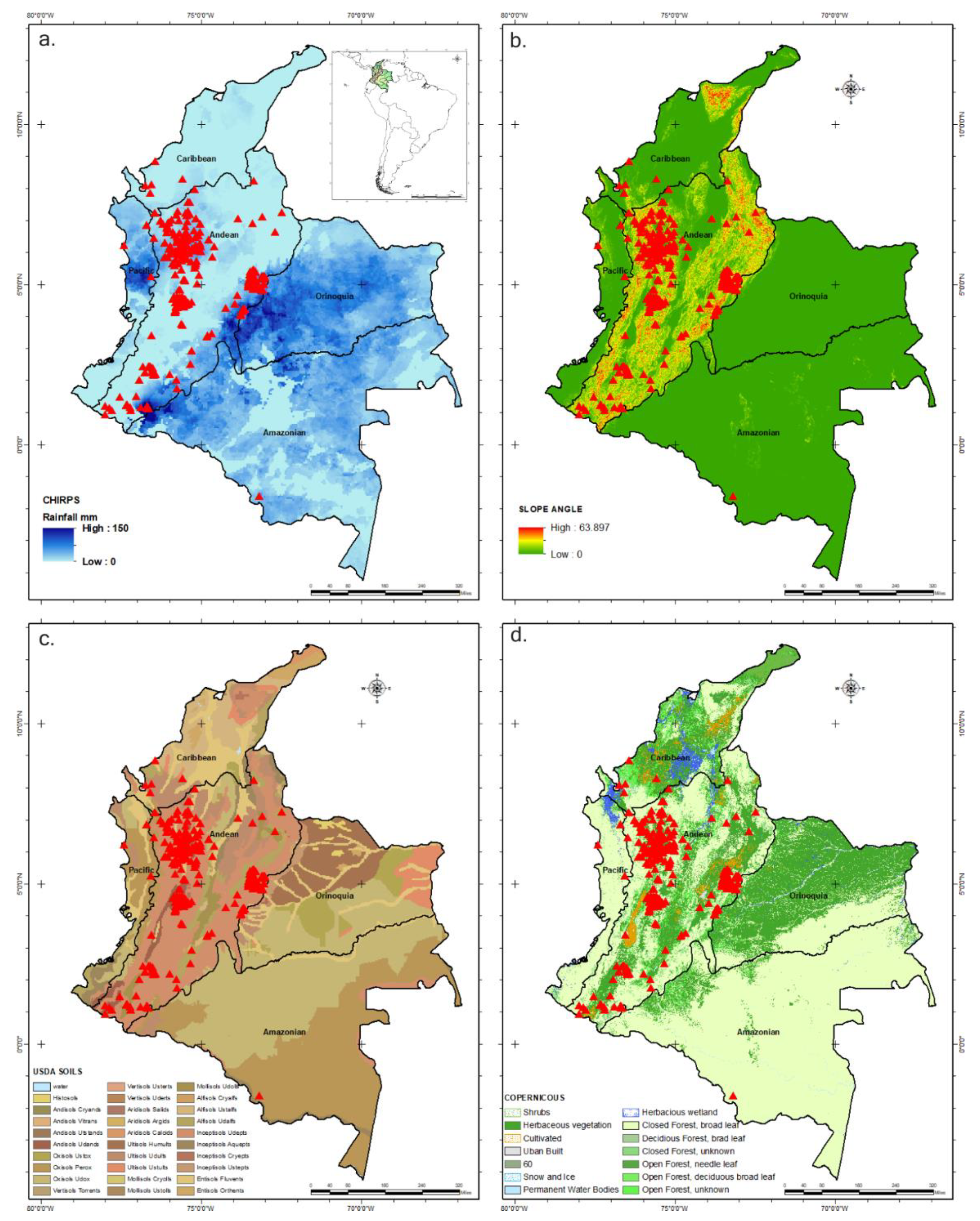
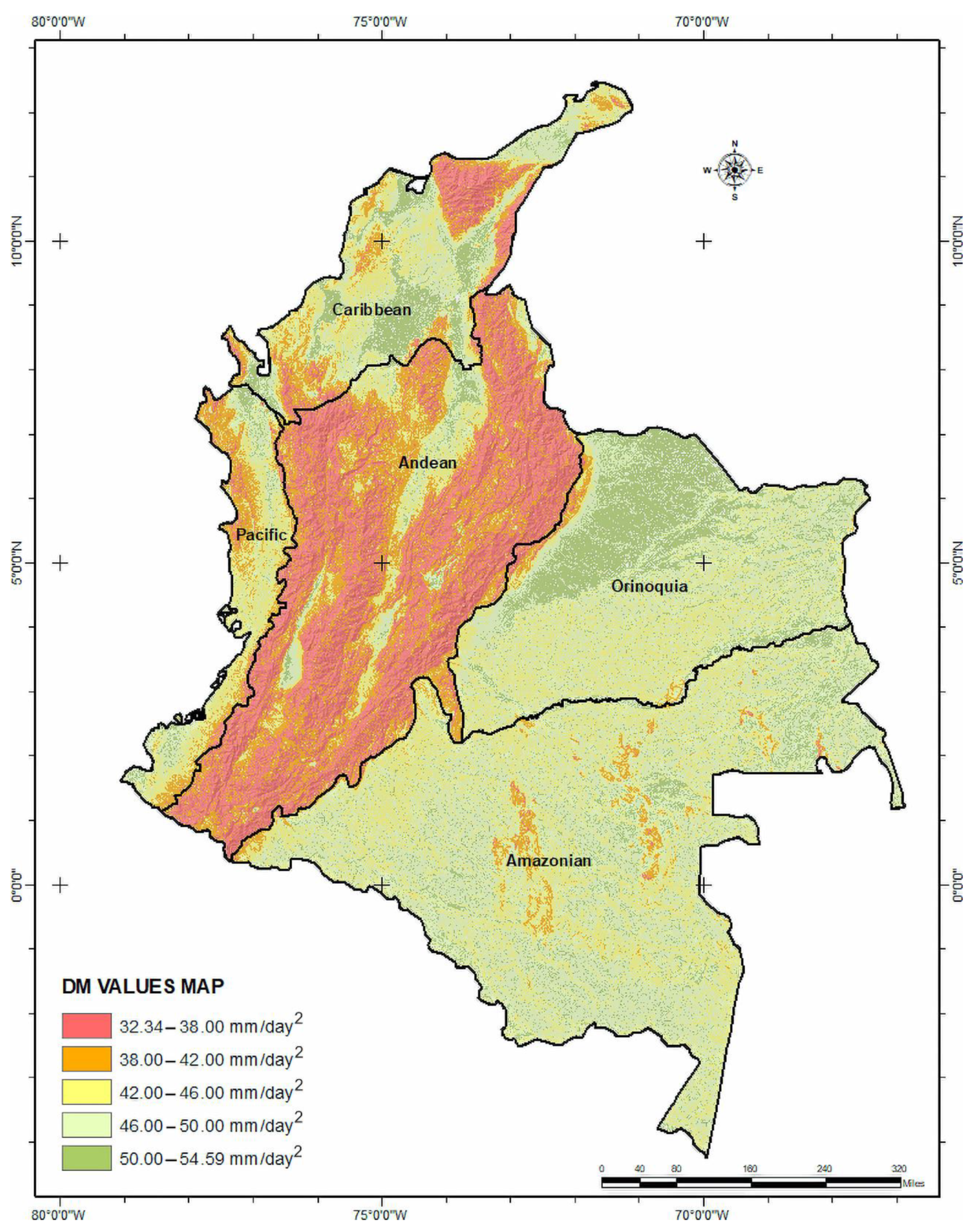
2.1. Geological and Climatological Settings

The country of Colombia is located in the northwest part of South America. It lies between latitudes 4°S and 12°N and longitudes 67°W and 79°W bordering Panama to the northwest; Brazil and Venezuela to the east; and Ecuador and Peru to the south. It is surrounded by the Caribbean Sea to the east and the Pacific Ocean to the west. According to the latest Colombian census of 2018, there are approximately 45,500,000 million residents in the country, many of whom inhabit the interior mountain ranges [22].

The Colombian Mountain ranges, or the Colombian Andes, are the result of subduction-accretion in the triple-plate junction of the Nazca, Caribbean, and South American plates, where tough terrains with steep slopes dominate the landscape. Moreover, these hillslopes are overlain by thick weathering profiles that consist of residual soils, saprolites, and weathered rock horizons. They are divided into three mountain ranges, known as the Western, Central, and Eastern mountains. Geomorphologically, it is a diverse country divided into five distinct natural regions: The Andean Mountain range, the Caribbean Sea coastal region, the Pacific Ocean coastal region, the lowlands of the Amazon, and the Orinoco region. The Andean Mountains have only 33% of the landmass, but 78% of the national population. This region also presents 92.5% of the total landslide reports, where 92% are triggered by rainfall [23].

Colombia has a tropical climate that exhibits a highly intermittent rainfall behavior in space and time. The mean annual precipitation over the whole country is 2830 mm [24]. Along the Andean region, the mean annual precipitation ranges from 1000 to 3000 mm, where strong topographic features produce local atmospheric circulations and convective rainstorm events, which commonly trigger flash floods and landslides [25]. Additionally, the double migration of the Inter-Tropical Convergence Zone (ITCZ) strongly controls the bimodal regime of rainy periods. This pattern is mainly observed in central and western Colombia where rainfall peaks are prominent in the months of March-April-May (MAM) and September-October-November (SON) [26]. The interannual rainfall variability is controlled mainly by El Niño/Southern Oscillation (ENSO). During El Niño, there is a decrease in precipitation and mean monthly flow of Colombia’s rivers as well as a decrease in soil moisture, whereas La Niña is generally associated with positive precipitation anomalies [27].

The Colombian territory is a complex tectonic setting under extreme hydro-meteorological conditions. These conditions create a multi-hazard landscape where geomorphological phenomena such as landslides, debris flows, earthquakes, and flooding are frequent. The Andes mountains that cross Colombia from south to north, for example, make the country extremely vulnerable to landslides. On Saturday, 1 April 2017, the Mocoa landslide is just one illustration of a heavy rainfall-triggered event in Colombia. More than 300 people were killed, 400 were injured, and the city was destroyed [28]. Later in the same month, on 20 April 2017, another landslide, in a different region, resulted in at least 17 deaths and dozens injured [29]. Although significant, these are just a few examples of the vast occurrence of landslide events in the region; Aristizábal and Sanchez (2020) recorded 32,022 landslides occurring in the 116 years between 1900 and 2016. Out of these events, 93% occurred in the Colombian Andes region, and 92% were landslides triggered by rainfall.

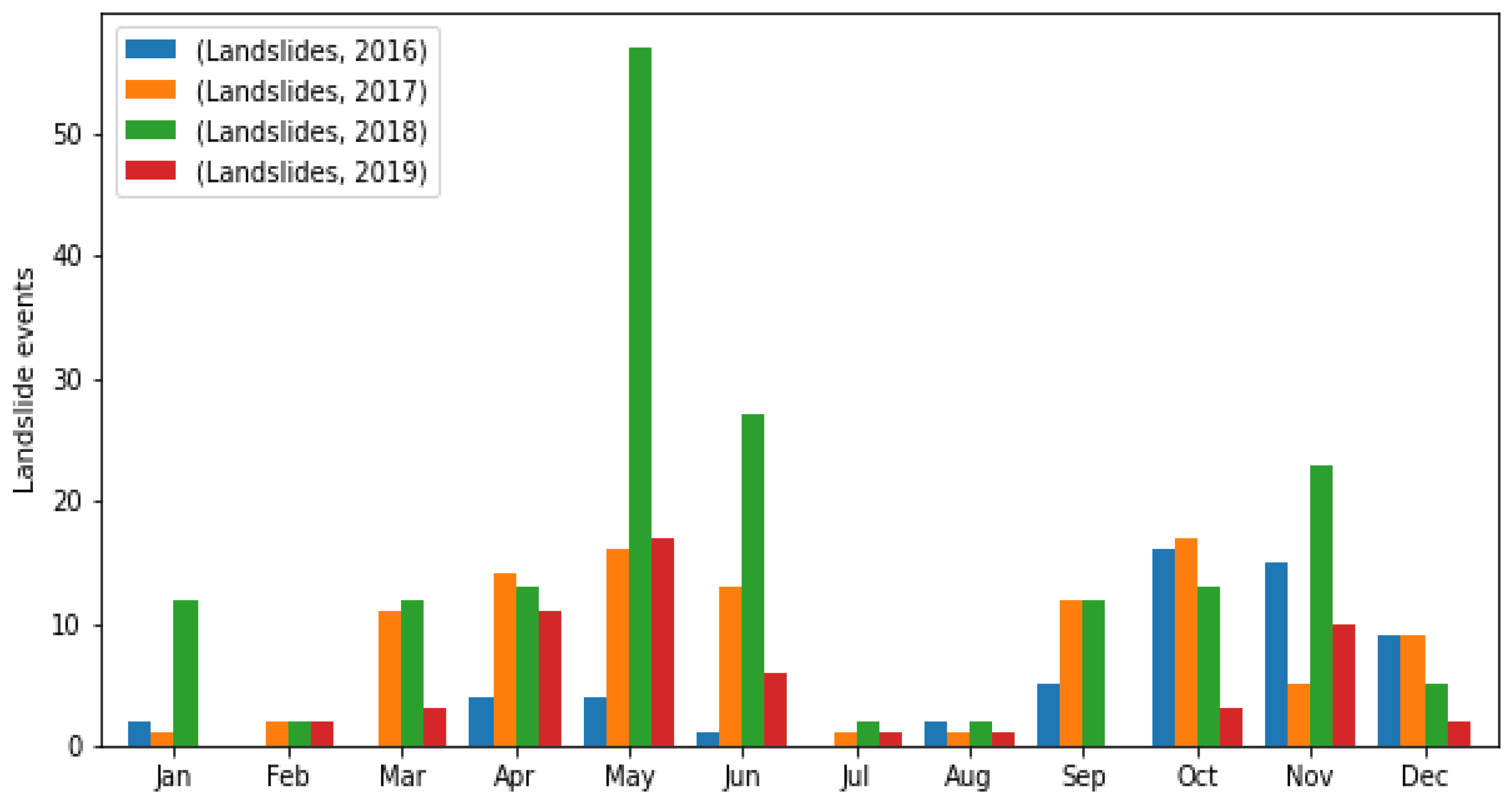
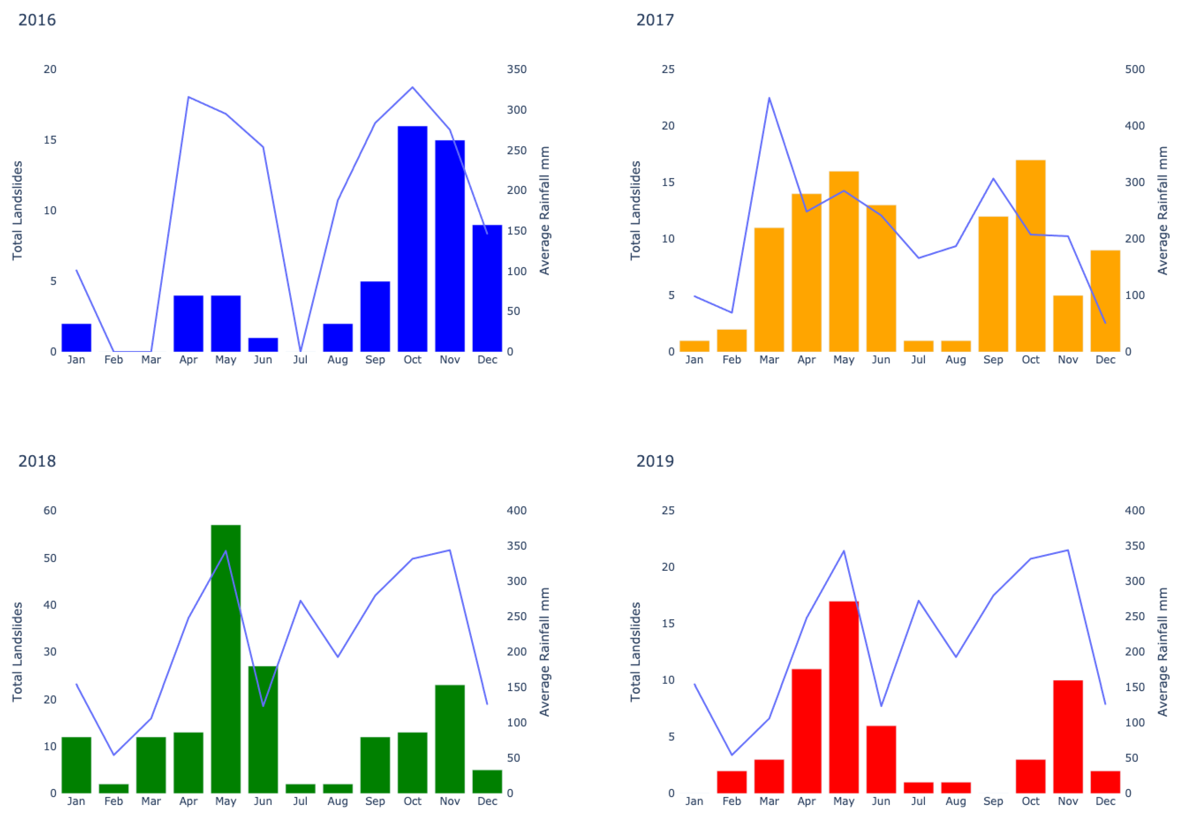
2.2. Landslide Inventory

El Servicio Geológico Colombiano (SGC) (https://simma.sgc.gov.co, accessed on 5 May 2020) and the National University of Colombia (https://geohazards.com.co/, accessed on 5 May 2020) keep landslide records in inventories for the Colombian territory. Both these registers are used in this work in such a way that one helps complement the other for the basis of evaluating static parameters. There were 396 landslides between the years 2016 and 2019 in Colombia, 346 triggered by rain, some of which resulted in numerous fatalities. For this work, each landslide event listed in the inventories is converted into a Geo Information System (GIS) point format for geo-location and corresponding retrieval of parameters.

Figure 1 below shows landslide events occurring between 2016 and 2019 as listed in these inventories. A bimodal annual pattern of landslide occurrence is observed in the data, with two maximum peaks in May and October-November, reflecting the strong influence of rainfall on landslide occurrence.

2.3. Static Parameters

Slope gradient is invariably one of the most significant physical parameters as shown by the various heuristic, statistical, and deterministic analyses in C.J. van Western (2008). In this work, slope angles are derived from NASA’s Shuttle Radar Topography Mission (SRTM) V3 [30]. SRTM provides digital elevation information at a 30 m resolution. We obtain the slope angle measurements using Google Earth Engine and extract slope angle values for each of the landslide event points.

Landcover of the study area was attained from the Copernicus Global Land Cover Layers: CGLS-LC100 Collection 3 (CGLS). The Copernicus information compiles a global landcover map at 100 m spatial resolution based on a database of landcover training sites and ancillary datasets. Copernicus released a landcover map for each year in the 2015–2019 period. Copernicus provides up to 80% accuracy over all the years of analysis [31]. Landcover information was also retrieved using Google Earth Engine and similarly corresponding event values are set aside in the landslide inventory database.

Major soils distribution for the study area was acquired from the United States Department of Agriculture (USDA), the National Cooperative Soil Survey (NCSS) [32] in GeoTiff format, and the Colombian Instituto Geográfico Agustín Codazzi (IGAC) [33] in shapefile format. These maps provide information at scale: 1:5,000,000 and 1:100,000, respectively. We use both these datasets to corroborate and complement soil characteristics but select major categories as described in the USDA format. We use ArcGIS 10.7 to extract values corresponding to each one of the landslide events.

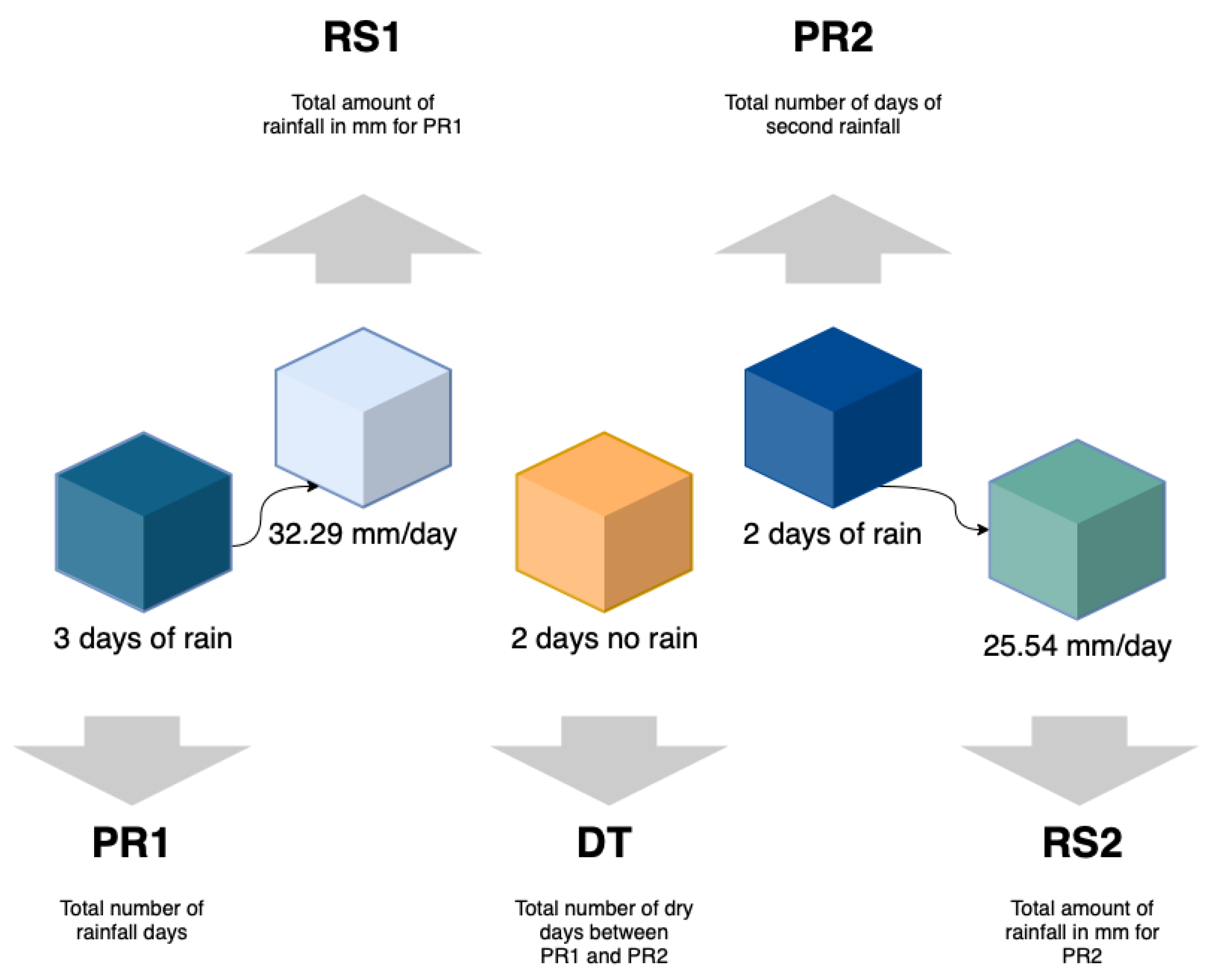
2.4. Dynamic Parameters

It is well established that rainfall intensity and duration can trigger shallow landslide activity [8,34]. Tropical areas that climatologically are more exposed to extreme rainfall events are usually located at the top of mountainous catchments. Not surprisingly, civil infrastructure and human settlements are very common along the gentle surfaces of these mountainous areas, which are composed of alluvial sediments in the lower catchments close to the mouth.

Although various satellite products are available to retrieve rainfall information globally, accurate measurements in tropical regions are usually hindered by dense vegetation that prevents the instruments from retrieving reliable readings. For this reason, data that are from a hybrid between satellite and ground instrumentation present an opportunity to remotely study rainfall dynamics in these areas.

The Climate Hazards Group Infrared Precipitation with Stations (CHIRPS) effort was developed by the United States Geological Survey (USGS) and the Climate Hazard Group (CHG) at the University of California Santa Barbara (USCB) to support the United States Agency for International Development Famine Early Warning System Network (FEWS NET). CHIRPS builds on various thermal infrared (TIR) precipitation products, calibrates global cold cloud duration rainfall estimates with the Tropical Rainfall Measuring Mission Multi-Satellite Precipitation Analysis version 7 (TMPA 3B42 v7), and uses various interpolated gauge products. CHIRPS data are available globally from 6-hour to 3-month aggregates at a 0.050 × 0.050-degree spatial resolution [35]. CHIRPS has been validated for Colombia. At least 338 rain gauges from the Colombian Instituto de Hidrología, Meteorología y Estudios Ambientales (IDEAM) were used to compare CHIRPS results, and correlations of R = 0.97 were reported accompanied by the benefit of relatively low latencies [35].

For this work, CHIRPS Daily: Version 2.0 Final was retrieved using Google Earth Engine. Daily precipitation between 2016 and 2019 was obtained for each latitude and longitude landslide point in the inventory.

Table 1. Datasets used in this work.

Data Type	Dataset	Resolution/Accuracy	Extent	Source
Slope	SRTM	30 m	Global	NASA/USGS/JPL-Caltech
Landcover	Copernicus	100 m	Global	Copernicus
Soils	USDA	1:5,000,000	Global	USDA
Rainfall	CHIRPS	0.05° × 0.05°	Global	UCSB/CHG
Landslide inventory	Universidad Nacional De Colombia/SGC	Various mapping scales and survey types	National	Universidad Nacional De Colombia/SGC

below describes all the static and dynamic datasets used in this study, and Figure 2 shows them in the study area.

The landslide inventories used in this work are maintained by the SGC and the Universidad Nacional and are two of the most complete in Colombia. For the 2016–2019 period, they list 346 rainfall triggered landslides. Both inventories are complemented with field campaigns that provide detailed descriptions of the events. However, landslide inventories are usually not free of inaccuracies that challenge the use of statistical methods to determine relationships between factors that can lead to a landslide event. This process becomes more intricate at the regional level because the related spatial and temporal data are extracted from remote sensors. Figure 3 below shows rain triggered landslide occurrence as listed in the inventory in the study area and the respective average cumulative rainfall for those events derived from CHIRPS. A remarkable peak in the number of landslides and rainfall in May 2018 is observed. This period corresponds to a strong La Niña ENSO event as reported in the Multivariate ENSO Index (MEI) [26].

3. Methods

3.1. Dynamic Factors Modeling—Soil Moisture and Rainfall

For the basis of this analysis, we assume that soil moisture content for a specific location is dependent on the amount and duration of the rainfall that occurs before the landslide event and in the non-rain (dry) periods between rainfall episodes. By following the successive rainfall/dry periods, we can characterize how much moisture is left in the soil directly before the landslide. A rainfall series for each landslide event location for 4 years (starting on 1 January 2016 and ending on 31 December 2019) is used to find precipitation characteristics for every two successive rainfall episodes as described in

Table 2. Variables created to track rainfall days, dry days, and rainfall amounts leading to a landslide event in the inventory.

Variable Name	Represents
PR1	Total number of days of Precedent Rainfall event
RS1	Rainfall Sum during PR1 in mm
PR2	Total number of days of rainfall event following PR1
RS2	Rainfall Sum during PR2 in mm
DT	Non-rainfall day period between two consecutive rainfall events

and illustrated in Figure 4 below.

As we investigate the rainfall/dry periods for each landslide location throughout the 4 years, we obtain approximately 125,901 data lines of RS1, RS2, PR1, PR2, and DT pairs.

Table 3. Example of rainfall/dry periods for one location from the beginning of the time series until the moment of the event—one landslide.

PR1 (Days)	RS1 (mm/Day)	DT (Days)	PR2 (Days)	RS2 (mm/Day)
1	34.30	2	1	34.30
1	34.30	1	3	52.31
3	52.31	27	1	11.87
1	11.87	3	1	6.00
1	6.00	2	1	8.17
…	…	…	…	…

below shows an example of the successive rainfall/dry periods for one location.

Consequently, we look for the two successive rainfall occurrences that lead to each one of the landslide events in the inventory. We investigate the rainy and dry periods right before the event and generalize them in Equation (1) as Pre-event Moisture Content.

$$\mathrm{PMC}=\frac{\mathrm{RS}1}{\mathrm{PR}1\ast \mathrm{DT}}$$

(1)

where PMC is an indicator factor of the moisture content in the soil before the landslide event and it is deemed as a first landslide triggering condition. Theoretically, any high values of RS1, associated with low PR1 and DT values, will increase the probability of a landslide event and therefore increase the PMC value.

The second condition is the triggering rainfall episode when the landslide happened, expressed in Equation (2) as Rainfall Sum Trigger.

$$\mathrm{RST}=\frac{\mathrm{RS}2}{\mathrm{PR}2\ast \mathrm{DT}}$$

(2)

where RS2 and PR2 are as described above. Mathematically, the RST value will be higher for higher RS2 associated with a low PR2 value. With a higher RST value, the soil will receive a higher amount of rainfall in a shorter period, therefore increasing the possibility of a landslide event.

3.2. Logistic Modeling—Dynamic and Static Factors

In this study, we define rainfall-triggered landslide susceptibility as the probability that a downslope movement would occur with rainfall as a trigger, but we also consider the pre-existing factors that underlie the physical characteristics of the region. We employ a stochastic approach in the form of logistic regression to understand the relationships between the newly derived dynamic variables, (PR1, RS1, PR2, RS2, and DT), some of the most important static factors (Slope, Landcover, and Soil type), and the landslide probability for the region. We use a logistic regression algorithm because it is a straightforward method for when some of the predictor variables are categorical [36]. The logistic regression method differs from the linear one in that the dependent variable is binary and represents a probability of the outcome. In our case, 1—landslide and 0—no landslide. This dichotomy makes the logistic regression approach a simple and helpful process to delineate landslide susceptibility as demonstrated by the numerous applications in various settings [9,36,37,38,39,40,41,42,43,44,45,46].

The logistic model can be, in its simplest form, as indicated in Equation (3), where the “log-odds” is denoted by Z, which depends linearly on the dynamic and static variables. The coefficients of this dependency are estimated in Section 4.1, using maximum likelihood estimation (MLE).

$$\mathrm{Probability} \left(\mathrm{Landslide}=1\right)=\frac{1}{1+{\mathrm{e} }^{-\mathrm{z}}}$$

(3)

In Equation (3), as Z increases, the probability of a shallow landslide event increases and vice-versa.

Four-years of rainfall data on each landslide location resulted in several (125,901) sets of dynamic values as explained above in Section 3.1. However, many of these values did not lead to the landslide event. For the proper setting of logistic regression, there were too many no-landslide to landslide values; the ratio was 93:7. Performing a logistic regression under these conditions would result in an erroneous predictive accuracy; therefore, we employed an under-sampling technique known as Synthetic Minority Under-Sampling Technique (SMOTE). SMOTE is an under-sampling method where the larger class is under-sampled by randomly selecting examples [47]. The resulting data for modeling had a 1:1 ratio of 1—landslide to 0—no-landslide. We use a Python subroutine that calculates the logistic regression for all dynamic and static variables.

Using training data for model assessment is not acceptable for evaluating the model’s performance in machine learning processes. Hence, we divide the landslide and no-landslide datasets into two groups: one for training, with approximately 70% of the data, and one for testing with the remaining 30%, as shown in

Table 4. Training and testing data—under sampling SMOTE.

Event	Cases	Under SMOTE	Cases Training	Cases Testing
1	346	346	241	105
0	125,901	346	238	108
Percentage	100%	100%	~70%	~30%

below.

The receiver-operating characteristic plot (ROC) is a solid logistic regression model performance evaluation, as it classifies the sensitivity (true positive rate) and the specificity (true negative rate) of the model. A model with high discrimination ability possesses high sensitivity and specificity simultaneously. Therefore, the area-under-ROC (AUC) grants the evaluation of thresholds in the model.

3.3. Landslide Thresholds

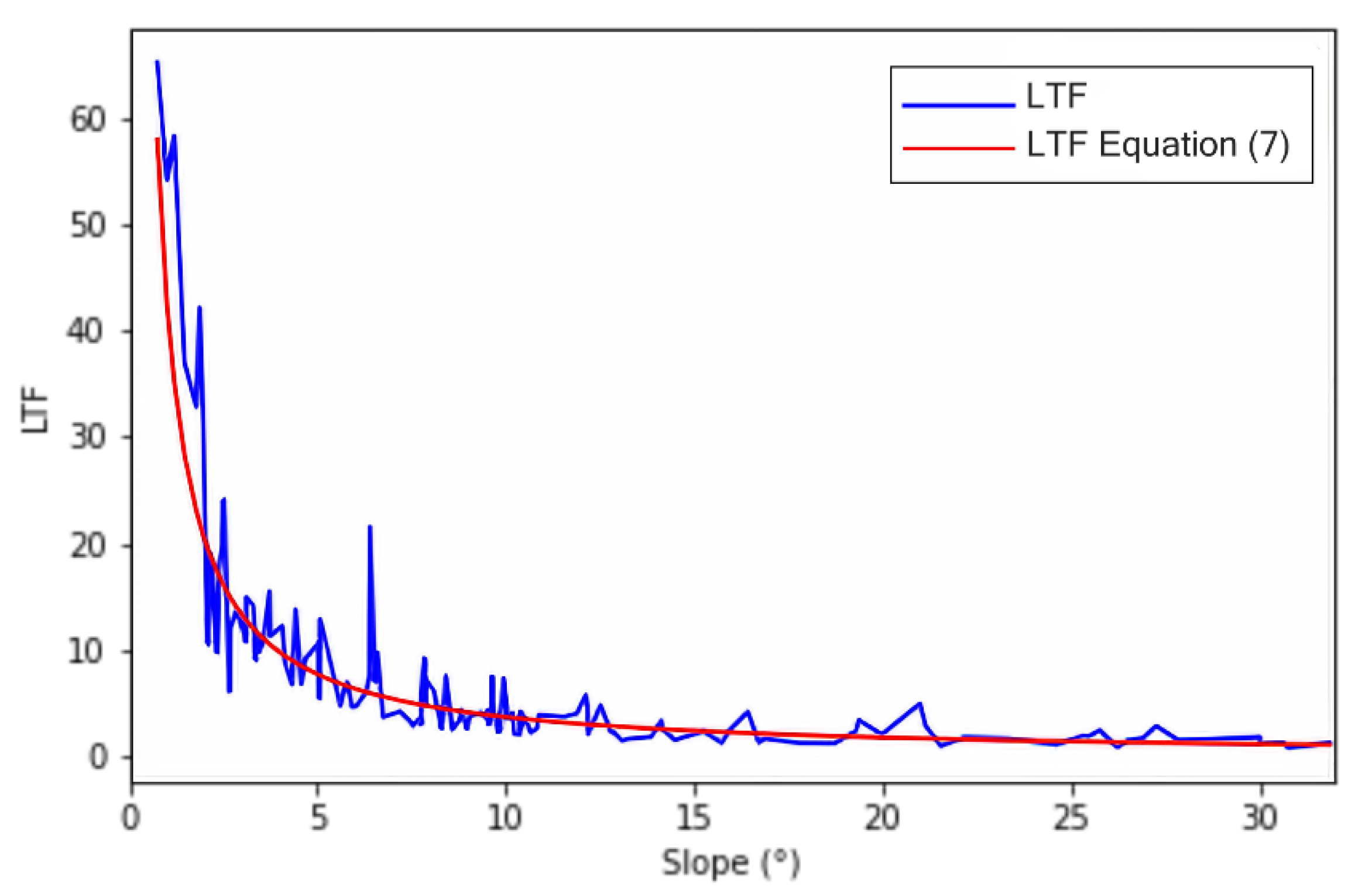
3.3.1. Landslide Triggering Factor—LTF

We integrate the two activating conditions PMC and RST into a landslide triggering factor LTF and normalize it by the slope angle parameter under the premise that as the slope increases, the amount of rainfall necessary to trigger a landslide event will decrease and vice-versa. In this manner, the LTF simply describes the relationship between the expected antecedent moisture content in the soil PMC and the rainfall RST that, according to the landslide inventory, triggered the event. The LTF can be seen in its equation form in Equation (4) below:

$$\mathrm{LTF}=\frac{\mathrm{PMC} + \mathrm{RST}}{\mathrm{Slope}}$$

(4)

where PMC and RST are as described above.

Equations (1), (2), and (4) were developed in this work to satisfy the mathematical probability of a landslide occurring. With the LTF, when the dynamic variables PMC and RST for a given slope angle increase, the probability of a landslide event increases as well. In contrast, as the dry period between the two successive rainfall occurrences (DT) increases, the probability of a landslide decreases.

3.3.2. Cumulative Rainfall Event-Duration (E-D) Threshold

The intensity or duration of rainfall periods can be used to establish statistical or empirical correlations to shallow landslide occurrence. These relationships are often expressed as rainfall thresholds that once exceeded, will cause a landslide [48]. The intensity-duration (I-D) threshold, for example, relates these quantities in a power law (I = αD^−b, where I is the rainfall mean intensity in mm/h; D is the duration of the rainfall event expressed hourly or daily; α is the scaling constant; and b represents the slope) [9].

Contrary to the I-D method, the event-duration (E-D) threshold does not consider the intensity, but instead, the total or cumulative rain. The cumulative precipitation event E is expressed as the total rain from beginning to end that triggered the landslide event. In the literature, various authors have expressed the E-D threshold in a similar power function to the I-D as shown in Equation (5a), where E is measured in (mm) for the full precipitation period; D is the duration of the rainfall episode, and it is expressed hourly or daily; α is the rainfall depth; and γ is the threshold inclination generated from the power function regression [13]. Similarly, the E-D threshold linear form was introduced by Valenzuela et al. (2019) as per Equation (5b) below:

$$\mathrm{E}={\mathsf{\alpha }\mathrm{D}}^{-\mathrm{\gamma }}$$

(5a)

$$\mathrm{E}+\mathsf{\alpha }\mathrm{D}=\mathrm{C}$$

(5b)

where E is the cumulative rain in (mm); D is the rainfall period expressed hourly or daily; α is the slope of the fitted line; and where C represents the y-intercept [49].

In this study, we evaluate both the power and linear functions but implement the E-D threshold in its linear form as a baseline to evaluate the LTF threshold performance. As previously noted, the landslide inventories used in this work do not provide the time, but the date of the event. In the lack of rainfall intensity information, the E-D threshold is most useful in this application. We also divide the dataset into a training group of approximately 65% and a testing group of approximately 35% for evaluating each of these methods.

3.4. Assumptions

Studying rainfall-triggered landslides at large scales using remote sensors and databases presents various challenges due to the non-structured nature of the information. In this study, it is important to highlight the following:

• Both the logistic regression model and the LTF threshold are data driven approaches.
• We assume that pore pressure increases due to liquefaction of the material.
• We suppose that soil moisture content for a specific location is dependent on the amount and duration of the rainfall that occurs before the landslide event and on the non-rain (dry) period between the two events. We do not incorporate root uptake or evapotranspiration information.
• Daily rainfall temporal resolution is used because the landslide inventory lists a date, not a timestamp of when the event occurred.
• It is understood that a landslide changes the physical characteristics of the area. It may flatten the slope and remove the weak soil layer, which in return may change the landcover. Under these circumstances, the calculated LTF for that location no longer applies because conditions have changed.

4. Results

4.1. Logistic Regression—Dynamic and Static Factors

The estimated coefficients for each factor affecting the “log-odds” using the maximum likelihood estimate (MLE) in the logistic model is presented in the Z-factor for Equation (3) above:

$$\mathrm{Z}=-\left(0.33\mathrm{PR}1-0.01\mathrm{RS}1+1.87\mathrm{DT}+0.33\mathrm{PR}2-0.01\mathrm{RS}2+0.20\mathrm{slope}+0.90\mathrm{SoilType}\right)$$

(6)

In Equation (3), P tends to 1 as Z in Equation (6) increases. As Z increases, the probability of a shallow landslide event tends towards 1 (landslide). In contrast, as Z decreases, the probability tends to 0 (no-landslide). The relationship between the coefficients and the probability is expressed as positive (landslide) or negative (no-landslide).

Landcover and soil type are categorical variables with six and five categories, respectively, for the study area and are described in depth in H. Eswaran (2016) and Smets (2020), respectively. Because this is a data-driven model, we do not assign any weight to any soil or landcover type. Instead, we create dummy variables for each category at each location. After segregating meaningful types of these categories using the RFE process, we are left with those that either influence the event to occur or not. Those with positive coefficients have a positive relationship to event causation and vice versa.

Validation results of the logistic regression demonstrate that the model can correctly predict 73% of the cases using the newly created dynamic variables. Figure 5a shows the ROC curve that helps summarize the model predictability based on the area under the curve (AUC). The AUC reflects the probability that a randomly chosen actual landslide incident will have a high chance of classification as being an actual event. The model has an AUC of 0.73, suggesting good data-driven predictability for landslide events. Figure 5b shows the confusion matrix for the model. These values help explain the precision (true positive)/(true positive + false positive), recall (true positive)/(true positive + false negative), and F1-measure, which combines the precision and recall. These measurements can be seen in

Table 5. Precision, recall and F-measure.

Class	Precision	Recall	F1-Score
0	0.71	0.79	0.75
1	0.75	0.67	0.71

below.

The odds ratio (OR) demonstrates how a one-unit increase or decrease in a variable affects the odds of initiating a landslide event. In

Table 6. Odds Ratio.

Variable	Coefficients	OR
PR1	−0.33	0.718
RS1	0.01	1.013
DT	−1.87	0.153
PR2	−0.33	0.715
RS2	0.01	1.011
Slope	−0.20	0.851
Soil Type	−0.90	0.404

below we see that for one unit increase in PR1, we expect that there is 0.718 times increase in the odds of a landslide happening. The other independent variables can be interpreted the same way.

4.2. Landslide Triggering Factor (LTF) Thresholds—Dynamic Factors and Slope

The LTF value for the training (65%) and testing (35%) datasets is assessed using Equation (4) for every two rainfall/dry periods at each landslide location from 1 January 2016 to 31 December 2019. LTF values that are associated with an actual landslide event are set as thresholds for the corresponding slope angles. Equation (7) and Figure 6 below show the inverse function that relates the LTF and the Slope angle.

$$\mathrm{LTFThreshold}=42.91{ \mathrm{Slope}}^{-1.068}$$

(7)

where the determination coefficient (R²) for the LTF threshold-Slope relationship as per Equation (7) is R² = 0.836. Figure 6 shows that the LTF-Slope angle relation rapidly changes in smaller slope angles, whereas it barely fluctuates in larger ones. Slopes greater than 25° show an asymptote average threshold value of 1.227 with a standard deviation of 0.104.

The LTF-slope relationship is congruent with the physical mechanisms that drive rainfall-triggered landslides. Physically, a rainfall-triggered landslide develops as the moisture content of the soil and its pore pressure increase. The slope fails when the driving force along the slip failure surface is greater than the shear strength of the material and its cohesion [50]. In steep-slope angles, the weight of the soil along the slope surface is already significant. In this case, a small amount of additional water weight is likely to initiate a failure. This explains the low variation of the LTF in the high slope ranges. Alternatively, for small slope angles, the soil’s weight component along the slip surface that contributes to the slope failure is relatively small, and therefore, a substantial additional water weight component is needed to initiate a failure. Hence, for small slope ranges, the LTF exhibits more heightened variations.

Landslide Triggering Factor Error—False Positive Rate (FPR)

The false positive rate is defined as the probability of falsely rejecting the null hypothesis. In our case, it represents the negative cases in the data that were mistakenly reported as positive or where the LTF threshold was exceeded but there was no landslide event. Consequently, we use the FPR concept to check the adequacy of the LTF threshold value as per Equation (8) below:

$$\mathrm{FPRLTF}=\frac{\mathrm{LTFOver}}{\mathrm{TotalPeriods}-1}$$

(8)

where LTFOver are the times in the rainfall series where the LTF value exceeded the established LTF threshold. TotalPeriods are the total number of rainfall/dry periods from the first day of the rainfall series to the actual landslide event. In this case, the maximum observed FPR value for all training cases was 0.271, demonstrating a 73% overall accuracy. Similarly, the testing dataset, 35% of the cases, presented a maximum FPR of 0.274 showing an overall performance of 72.6%.

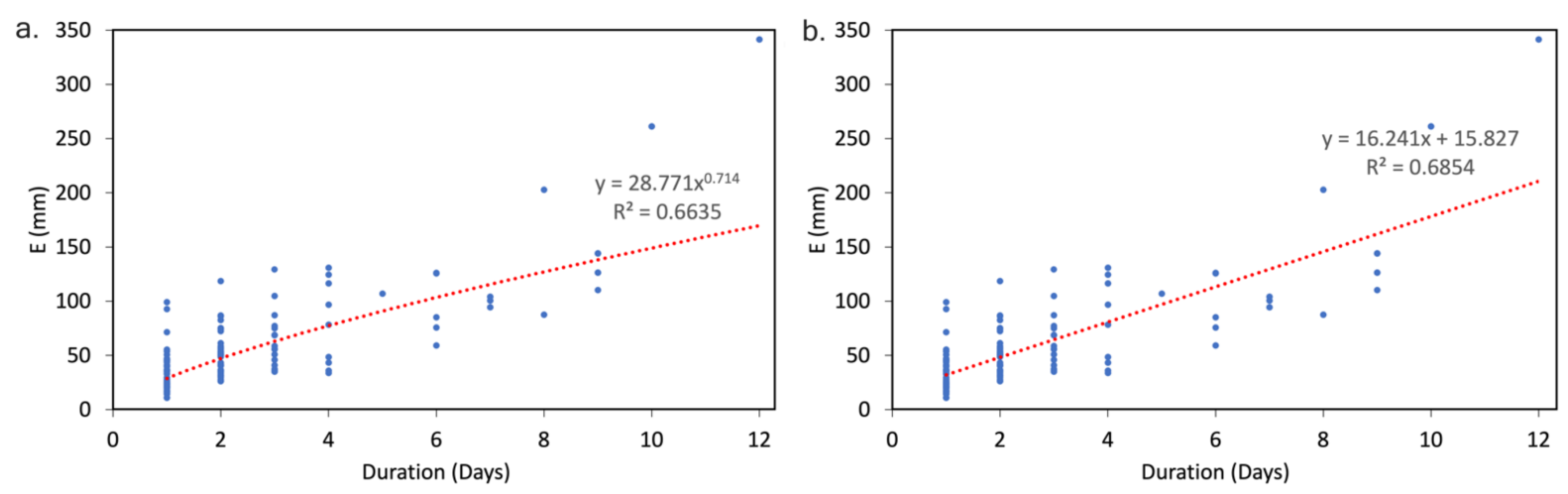
4.3. Accumulated Rainfall Duration (E-D) Threshold—Dynamic Factors and Slope

The E-D values in the power and linear forms for the training dataset are shown in Figure 7a,b below. In these Figures, the E-D threshold values are fitted with the corresponding E-D linear and power forms as per Equations (5a) and (5b) above.

For each instance, the corresponding curve becomes as per Equations (9a) and (9b).

$$\mathrm{EDThreshold}=28.77{ \mathrm{D}}^{0.714}$$

(9a)

$$\mathrm{EDThreshold}=15.83+16.24 \mathrm{D}$$

(9b)

Equations (9a) and (9b) define whether a landslide event happens or not. Here, for an observed accumulated rainfall (E) for a time duration (D), if E is greater than the threshold, a landslide should be expected. However, in this case, the linear form exhibits a higher determination coefficient (R² = 0.68), thus, we use this form.

Accumulated Rainfall Duration (E-D) Thresholds Error—False Positive Rate (FPR)

We calculate the E-D threshold false positive rate (FPR) using the same approach as for the LTF FPR. In Equation (10) below, we substitute LTFOver for EDOver from Equation (8) above.

$$\mathrm{FPRED}=\frac{\mathrm{EDOver}}{\mathrm{TotalPeriods}-1}$$

(10)

where EDOver are the times in the rainfall series where the E value exceeded the established E-D threshold, and TotalPeriods are the total number of rainfall/dry periods from the first day of the rainfall series to the actual landslide event. In this case, the maximum observed FPR value for all training cases was 0.60.

4.4. LTF Threshold vs. E-D Threshold

It is well known that the antecedent moisture conditions of the soil before a landslide event are critical for landslide initiation. Regardless of the intensity and duration of a rainfall episode, shallow landslides are directly affected by soil moisture conditions [51,52]. Various physically based analyses have demonstrated that slope instability does not only depend on the intensity of the rain or its duration. It is the case that extensive precipitation within a dry period can trigger a landslide as much as a low-intensity rainfall during a wet period [53]. Similarly, pre-existing wet conditions can cause large debris flow during or following a downpour [54].

The E-D method uses the duration and accumulation of the triggering rainfall to establish a threshold value that, once exceeded, will lead to a landslide event. The LTF method, instead, not only considers the triggering rainfall but also evaluates the effects of the preceding precipitation before the triggering rain and the dry period in between the two rainfalls. The maximum observed FPR for the E-D method for the training dataset was 0.60. Conversely, the LTF FPR was 0.271 as noted above.

Figure 8a,b below show the E-D and LTF threshold FPR values for the training and testing datasets. In both cases, the LTF threshold performs better than the E-D threshold for 71% and 81% of the cases, respectively.

The difference in performance between the two thresholds can potentially be explained by the introduction of parameters that simulate the state of the soil before the landslide event and by relating them to the slope inclination. The LTF method considers five dynamic variables (RS1, PR1, RS2, PR2, and DT) that precariously simulate the wet state of the soil before the landslide event affecting the probability of a landslide. This assumption is possible under the notion that the slope angle inclination is inversely proportional to the amount of rainfall necessary to trigger a landslide. Conversely, by design, the E-D threshold does not consider any information about the soil wetness pre-event, therefore limiting its performance.

4.5. Landslide Triggering Factor—(LTF) Thresholds Hazard Map

A landslide hazard map that shows the probability of where and when an event would happen, as defined by Guzzetti et al. (2005) [55], can be derived by applying the LTF threshold concept to the slope angle distribution in the study area. From Equation (4) above, we can now derive a dynamic value that can be mapped for all areas where the quantities of both rainfall periods (RS1, RS2), their duration (PR1, PR2), and the dry period in between (DT) exceeds the LTF threshold as follows:

$$\mathrm{DynamicMap} \left(\mathrm{DM}\right); \mathrm{LTF} > \mathrm{LTFThreshold}$$

(11)

By defining DM as in Equation (11):

$$\mathrm{DM}=\frac{\mathrm{RS}1}{\mathrm{PR}1\ast \mathrm{DT}}+\frac{\mathrm{RS}2}{\mathrm{PR}2\ast \mathrm{DT} }$$

(12)

And then substituting Equations (4), (7), and (10) into Equation (11) and simplifying:

$$\mathrm{DM} >42.91{\ast \mathrm{Slope}}^{-0.068}$$

(13)

The DynamicMap (DM) quantities represent the average rainfall in mm/day of the two rainfalls divided by the dry period between the two rainfalls in days. In Figure 9 below, it is anticipated that when the DM quantity exceeds the LTF threshold multiplied by the slope, a landslide should be expected. Areas located in the mountainous Andes region show relative low DM (Equation (12)) values necessary to trigger a landslide. This is evident, as the area is characterized by high slopes. Conversely, areas located in the Caribbean Sea coastal region, the Pacific Ocean coastal region, and the lowlands of the Amazon and Orinoco regions with gentle or very low slopes require higher DM values.

The DM values map highlights the Andes region as the area that is at most risk of landslides with lower DM threshold values. From a risk management perspective, new DM values can be derived from weather forecasts where a landslide should be expected if the new calculated DM values overpass the DM thresholds presented here.

4.6. Challenges and Limitations

It is important to highlight the limitations of this work. First, the landslide records on which this work was based do not provide a timestamp of the event. For this reason, a daily average of rainfall estimates is used to develop both the logistic model and the LTF thresholds. Information that reflects the exact time of the event could have a significant impact on the LTF and DM thresholds. CHIRPS, for example, provides rainfall information every 6 h, and having a landslide inventory that gives a time of event could be useful to improve performance.

Second, because of the lack of satellite-based antecedent soil moisture information for the study area, wet and dry periods are used to simulate the effect that antecedent soil wetness would have in landslide initiation. This point itself is a significant assumption, as all the intrinsic physical dynamics of soil moisture conditions are not accounted for. Furthermore, this notion is based on rainfall estimates, and although these approximations have demonstrated high correlations with in-situ gauges, they have their limitations and uncertainties. Consequently, they have a direct effect on the LTF and DM thresholds.

Finally, although the DM map could serve as guidance for the landslide rainfall threshold, it is essential to note that the DM map is based on a 30 m resolution, but many landslides occur at smaller scales.

5. Conclusions

Rainfall-triggered landslides are a significant and constant hazard for the Andes region. This danger, coupled with the lack of availability of on-site instrumentation and the reliability of remotely sensed information, opens the need for more imaginative ways to unravel the problem. We present a data-driven solution in the form of dynamic variables derived from a satellite infrared precipitation and station data, CHIRPS, to simulate soil moisture variations and build a landslide triggering threshold in the Colombian region.

With the assumptions detailed above, we study four years of daily rainfall at 346 landslide events in the region. We focus on the two consecutive rainfall occurrences and corresponding dry periods leading to each one of the landslide events in the inventory. We then use them as dynamic variables. We first investigate the relationship of these rainy/dry periods in a logistic algorithm where results demonstrate acceptable performance of 73%.

Consequently, we take the rainy and dry periods right before the landslide event and simplify them as the PMC value. This value serves as an indicator for the moisture content in the soil before the landslide event. The triggering rainfall episode is then expressed as the RST value. Accordingly, these two factors are normalized with the effect of the slope angle giving rise to the LTF concept.

The LTF model allows for the allocation of threshold values associated with slope angles, and we see that as the slope increases the LTF decreases. The LTF also serves as a guidance for landslide hazards in the region, as areas with lower threshold values and high slopes are at a higher risk of landslides and vice-versa.

Although the simulated LTF lacks details about the complex processes that drive soil moisture mechanics, it attempts to simulate them by including the triggering rain, the antecedent rainfall, and the dry period in between. When the LTF is compared to the E-D threshold, the LTF performs better for 81% of the testing cases.

Although various physically based landslide rainfall thresholds have been developed for the study area, no satellite-based thresholds currently exist. The LTF threshold is one of the first satellite-based thresholds for the Colombian region that attempts to simulate the effect of this parameter in the area.

DM values for the Andes region range between 32 and 46 mm/day² mark this as the region with the least precipitation (in two rainfall episodes) necessary to trigger a landslide. And although the DM map could serve as a guide for vulnerability and risk, several challenges should be resolved to “fine-tune” the thresholds. These include introducing a “time of event” parameter and physical or reliable satellite-based antecedent soil moisture information when it becomes available.

References

1. Girty, G.H. Perilous Earth: Understanding Processes behind Natural Disasters, ver. 1.0 Chapter 8 Landslides. 2009. Available online: http://www.sci.sdsu.edu/visualgeology/naturaldisasters/ (accessed on 1 July 2021).
2. Petley, D. Global patterns of loss of life from landslides. Geology 2012, 40, 927–930. [Google Scholar] [CrossRef]
3. Kim, H.G.; Lee, D.K.; Park, C. Assessing the cost of damage and effect of adaptation to landslides considering climate change. Sustainability 2018, 10, 1628. [Google Scholar] [CrossRef] [Green Version]
4. Cruden, D.J.; Varnes, D.M. Landslides: Investigation and Mitigation. Transp. Res. Board Spec. Rep. 1996, 247, 36–75. [Google Scholar]
5. Sidle, R.C.; Ochiai, H. Landslides: Processes, Prediction, and Land Use; American Geophysical Union: Washington, DC, USA, 2006; Volume 18. [Google Scholar] [CrossRef]
6. Kirschbaum, D.B.; Adler, R.; Hong, Y.; Lerner-Lam, A. Evaluation of a preliminary satellite-based landslide hazard algorithm using global landslide inventories. Nat. Hazards Earth Syst. Sci. 2009, 9, 673–686. [Google Scholar] [CrossRef] [Green Version]
7. Aristizábal, E.; García, E.; Martínez, C. Susceptibility assessment of shallow landslides triggered by rainfall in tropical basins and mountainous terrains. Nat. Hazards 2015, 78, 621–634. [Google Scholar] [CrossRef]
8. Aristizábal, E.; Velez, J.; Martínez, C.; Jaboyedoff, M. SHIA_Landslide: A distributed conceptual and physically based model to forecast the temporal and spatial occurrence of shallow landslides triggered by rainfall in tropical and mountainous basins. Landslides 2015, 13, 497–517. [Google Scholar] [CrossRef]
9. Cullen, C.A.; Al-Suhili, R.; Khanbilvardi, R. Guidance index for shallow landslide hazard analysis. Remote Sens. 2016, 8, 866. [Google Scholar] [CrossRef] [Green Version]
10. Collins, B.D.; Znidarcic, D. Stability Analyses of Rainfall Induced Landslides. J. Geotech. Geoenviron. Eng. 2004, 130, 362. [Google Scholar] [CrossRef]
11. Glade, T.; Anderson, M.; Crozier, M. Landslide Hazard and Risk; John Wiley & Sons, Ltd.: Hoboken, NJ, USA, 2004; Available online: https://books.google.com/books?id=UFQk0I4EUiwC&printsec=frontcover&source=gbs_ge_summary_r&cad=0#v=onepage&q&f=false (accessed on 22 March 2022).
12. Caine, N. The rainfall intensity-duration control of shallow landslides and debris flows. Geogr. Ann. Ser. A Phys. Geogr. 1980, 62, 23–27. [Google Scholar]
13. Maturidi, A.M.A.M.; Kasim, N.; Taib, K.A.; Azahar, W.N.A.W. Rainfall-Induced Landslide Thresholds Development by Considering Different Rainfall Parameters: A Review. J. Ecol. Eng. 2021, 22, 85–97. [Google Scholar] [CrossRef]
14. Dikshit, A.; Satyam, N.; Pradhan, B.; Kushal, S. Estimating rainfall threshold and temporal probability for landslide occurrences in Darjeeling Himalayas. Geosci. J. 2020, 24, 225–233. [Google Scholar] [CrossRef]
15. Naidu, S.; Sajinkumar, K.S.; Oommen, T.; Anuja, V.J.; Samuel, R.A.; Muraleedharan, C. Early warning system for shallow landslides using rainfall threshold and slope stability analysis. Geosci. Front. 2018, 9, 1871–1882. [Google Scholar] [CrossRef]
16. Mandal, P.; Sarkar, S. Estimation of rainfall threshold for the early warning of shallow landslides along National Highway-10 in Darjeeling Himalayas. Nat. Hazards 2021, 105, 2455–2480. [Google Scholar] [CrossRef]
17. Kirschbaum, D.B.; Stanley, T.; Simmons, J. A dynamic landslide hazard assessment system for Central America and Hispaniola. Nat. Hazards Earth Syst. Sci. 2015, 15, 2257–2272. [Google Scholar] [CrossRef] [Green Version]
18. Brunetti, M.T.; Melillo, M.; Gariano, S.L.; Ciabatta, L.; Brocca, L.; Amarnath, G.; Peruccacci, S. Satellite rainfall products outperform ground observations for landslide prediction in India. Hydrol. Earth Syst. Sci. 2021, 25, 3267–3279. [Google Scholar] [CrossRef]
19. Rossi, M.; Luciani, S.; Valigi, D.; Kirschbaum, D.; Brunetti, M.T.; Peruccacci, S.; Guzzetti, F. Statistical approaches for the definition of landslide rainfall thresholds and their uncertainty using rain gauge and satellite data. Geomorphology 2017, 285, 16–27. [Google Scholar] [CrossRef]
20. Marin, R.J.; Velásquez, M.F.; García, E.F.; Alvioli, M.; Aristizábal, E. Assessing two methods of defining rainfall intensity and duration thresholds for shallow landslides in data-scarce catchments of the Colombian Andean Mountains. Catena 2021, 206, 105563. [Google Scholar] [CrossRef]
21. van Westen, C.J.; Castellanos, E.; Kuriakose, S.L. Spatial data for landslide susceptibility, hazard, and vulnerability assessment: An overview. Eng. Geol. 2008, 102, 112–131. [Google Scholar] [CrossRef]
22. Vallejo-Zamudio, L.E. El incierto crecimiento económico colombiano. Apuntes Cenes 2017, 36, 9–10. [Google Scholar] [CrossRef] [Green Version]
23. Aristizábal, E.; Sánchez, O. Spatial and temporal patterns and the socioeconomic impacts of landslides in the tropical and mountainous Colombian Andes. Disasters 2020, 44, 596–618. [Google Scholar] [CrossRef] [PubMed]
24. Poveda, G.; Vélez, J.I.; Mesa, O.J.; Cuartas, A.; Barco, J.; Mantilla, R.I.; Mejía, J.F.; Hoyos, C.D.; Ramírez, J.M.; Ceballos, L.I.; et al. Linking Long-Term Water Balances and Statistical Scaling to Estimate River Flows along the Drainage Network of Colombia. J. Hydrol. Eng. 2007, 12, 4–13. [Google Scholar] [CrossRef] [Green Version]
25. Álvarez-Villa, O.D.; Vélez, J.I.; Poveda, G. Improved long-term mean annual rainfall fields for Colombia. Int. J. Climatol. 2011, 31, 2194–2212. [Google Scholar] [CrossRef]
26. NOAA—Physical Science Laboratory. Multivariate ENSO Index Version 2 (MEI.v2). NOAA ENSO. 2022. Available online: https://psl.noaa.gov/enso/mei/ (accessed on 25 February 2022).
27. Poveda, G. Diagnóstico del Ciclo Anual y Efectos del ENSO Sobre la Intensidad Máxima de Lluvias de Duración Entre 1 y 24 Horas en los Andes de Colombia. Meteorol. Colomb. 2002, 5, 67–74. [Google Scholar]
28. El Espectador. Avalancha en Mocoa, una de las Peores Tragedias de 2017. 2017. Available online: https://www.elespectador.com/noticias/nacional/avalancha-en-mocoa-una-de-las-peores-tragedias-de-2017/ (accessed on 19 October 2020).
29. Benfield, A. Global Catastrophe Recap. 2019. Available online: http://thoughtleadership.aonbenfield.com/Documents/20190508-analytics-if-april-global-recap.pdf (accessed on 4 July 2020).
30. Farr, T.G.; Rosen, P.A.; Caro, E.; Crippen, R.; Duren, R.; Hensley, S.; Kobrick, M.; Paller, M.; Rodriguez, E.; Roth, L.; et al. The shuttle radar topography mission. Rev. Geophys. 2007, 45, 2. [Google Scholar] [CrossRef] [Green Version]
31. Buchhorn, M.; Bertels, L.; Smets, B.; De Roo, B.; Lesiv, M.; Tsendbazar, N.E.; Masiliunas, D.; Linlin, L. Copernicus Global Land Service: Land Cover 100m: Version 3 Globe 2015–2019: Algorithm Theoretical Basis Document; Zenodo: Geneve, Switzerland, 2020. [Google Scholar] [CrossRef]
32. Eswaran, H.; Reich, P.; Padmanabhan, E. World soil resources opportunities and challenges. In World Soil Resources and Food Security; CRC Press, Taylor and Francis Group: Boca Raton, FL, USA, 2016; pp. 29–52. [Google Scholar]
33. Instituto Geográfico Agustín Codazzi- Subdirección de Agrología—Grupo Interno de Trabajo Geomática. Mapas de Suelos del Territorio Colombiano a Escala 1:100.000. 31 December 2017. Available online: http://metadatos.igac.gov.co/geonetwork/srv/spa/catalog.search#/metadata/b857e651-b8d2-4bf2-9e03-41a038c7206a (accessed on 14 August 2020).
34. Lehmann, P.; Gambazzi, F.; Suski, B.; Baron, L.; Askarinejad, A.; Springman, S.M.; Holliger, K.; Or, D. Evolution of soil wetting patterns preceding a hydrologically induced landslide inferred from electrical resistivity survey and point measurements of volumetric water content and pore water pressure. Water Resour. Res. 2013, 49, 7992–8004. [Google Scholar] [CrossRef]
35. Funk, C.; Peterson, P.; Landsfeld, M.; Pedreros, D.; Verdin, J.; Shukla, S.; Husak, G.; Rowland, J.; Harrison, L.; Hoell, A.; et al. The climate hazards infrared precipitation with stations—A new environmental record for monitoring extremes. Sci. Data 2015, 2, 150066. [Google Scholar] [CrossRef] [PubMed] [Green Version]
36. Gorsevski, P.V.; Gessler, P.E.; Foltz, R.B.; Elliot, W.J. Spatial prediction of landslide hazard using logistic regression and ROC analysis. Trans. GIS 2006, 10, 395–415. [Google Scholar] [CrossRef]
37. Guns, M.; Vanacker, V. Logistic regression applied to natural hazards: Rare event logistic regression with replications. Nat. Hazards Earth Syst. Sci. 2012, 12, 1937–1947. [Google Scholar] [CrossRef]
38. Thomas, D.R.; Zumbo, B.D.; Dutta, S. On Measuring the Relative Importance of Explanatory Variables in a Logistic Regression. J. Mod. Appl. Stat. Methods 2008, 7, 4. [Google Scholar] [CrossRef] [Green Version]
39. Zhu, L.; Huang, J. GIS-based logistic regression method for landslide susceptibility mapping in regional scale. J. Zhejiang Univ. Sci. A 2006, 7, 2007–2017. [Google Scholar] [CrossRef]
40. Akbari, A.; Bin, F.; Yahaya, M.; Azamirad, M.; Fanodi, M. Landslide Susceptibility Mapping Using Logistic Regression Analysis and GIS Tools. Electron. J. Geotech. Eng. 2014, 19, 1687–1696. [Google Scholar]
41. Regmi, N.R.; Giardino, J.R.; McDonald, E.V.; Vitek, J.D. A comparison of logistic regression-based models of susceptibility to landslides in western Colorado, USA. Landslides 2014, 11, 247–262. [Google Scholar] [CrossRef]
42. Lee, S. Cross-verification of spatial logistic regression for landslide susceptibility analysis: A case study of Korea. In Proceedings of the 31st International Symposium on Remote Sensing of Environment, ISRSE 2005: Global Monitoring for Sustainability and Security, St. Petersburg, Russia, 20–24 June 2005; Available online: http://www.scopus.com/inward/record.url?eid=2-s2.0-84879728712&partnerID=tZOtx3y1 (accessed on 4 March 2020).
43. Kavzoglu, T.; Sahin, E.K.; Colkesen, I. Landslide susceptibility mapping using GIS-based multi-criteria decision analysis, support vector machines, and logistic regression. Landslides 2013, 11, 425–439. [Google Scholar] [CrossRef]
44. Pourghasemi, H.R.; Moradi, H.R.; Aghda, S.M.F. Landslide susceptibility mapping by binary logistic regression, analytical hierarchy process, and statistical index models and assessment of their performances. Nat. Hazards 2013, 69, 749–779. [Google Scholar] [CrossRef]
45. Shahabi, H.; Khezri, S.; Ahmad, B.B.; Hashim, M. Landslide susceptibility mapping at central Zab basin, Iran: A comparison between analytical hierarchy process, frequency ratio and logistic regression models. Catena 2014, 115, 55–70. [Google Scholar] [CrossRef]
46. Ayalew, L.; Yamagishi, H. The application of GIS-based logistic regression for landslide susceptibility mapping in the Kakuda-Yahiko Mountains, Central Japan. Geomorphology 2005, 65, 15–31. [Google Scholar] [CrossRef]
47. Chawla, N.V.; Bowyer, K.W.; Hall, L.O.; Kegelmeyer, W.P. SMOTE: Synthetic Minority Over-sampling Technique. J. Artif. Intell. Res. 2002, 16, 321–357. [Google Scholar] [CrossRef]
48. Segoni, S.; Rossi, G.; Rosi, A.; Catani, F. Landslides triggered by rainfall: A semi-automated procedure to define consistent intensity–duration thresholds. Comput. Geosci. 2014, 63, 123–131. [Google Scholar] [CrossRef]
49. Valenzuela, P.; Zêzere, J.L.; Domínguez-Cuesta, M.J.; García, M.A.M. Empirical rainfall thresholds for the triggering of landslides in Asturias (NW Spain). Landslides 2019, 16, 1285–1300. [Google Scholar] [CrossRef]
50. Mathew, J.; Babu, D.G.; Kundu, S.; Kumar, K.V.; Pant, C.C. Integrating intensity-duration-based rainfall threshold and antecedent rainfall-based probability estimate towards generating early warning for rainfall-induced landslides in parts of the Garhwal Himalaya, India. Landslides 2014, 11, 575–588. [Google Scholar] [CrossRef]
51. Glade, T.; Crozier, M.; Smith, P. Applying probability determination to refine landslide-triggering rainfall thresholds using an empirical ‘Antecedent Daily Rainfall Model. Pure Appl. Geophys. 2000, 157, 1059–1079. Available online: http://link.springer.com/article/10.1007/s000240050017 (accessed on 14 August 2014). [CrossRef]
52. Liao, Z.; Hong, Y.; Wang, J.; Fukuoka, H.; Sassa, K.; Karnawati, D.; Fathani, F. Prototyping an experimental early warning system for rainfall-induced landslides in Indonesia using satellite remote sensing and geospatial datasets. Landslides 2010, 7, 317–324. [Google Scholar] [CrossRef]
53. Godt, J.W.; Baum, R.L.; Chleborad, A.F. Rainfall characteristics for shallow landsliding in Seattle, Washington, USA. Earth Surf. Processes Landf. 2006, 31, 97–110. [Google Scholar] [CrossRef]
54. Baum, R.L.; Godt, J.W. Early warning of rainfall-induced shallow landslides and debris flows in the USA. Landslides 2009, 7, 259–272. [Google Scholar] [CrossRef]
55. Guzzetti, F.; Stark, C.P.; Salvati, P. Evaluation of flood and landslide risk to the population of Italy. Environ. Manag. 2005, 36, 15–36. [Google Scholar] [CrossRef] [PubMed]
Figure 1. Landslide events in Colombia between 2016 and 2019.
Remotesensing 14 02239 g001
Figure 2. Datasets used for the study area and corresponding landslide events happening between 2016 and 2019: (a) CHIRPS rainfall (mm)—used in the logistic model and LTF method; (b) slope angle derived from SRTM V3—used in the logistic model and LTF method. (c) USDA Soils Classification—used in the logistic model; (d) Copernicus Landcover 2019—used in the logistic model.
Remotesensing 14 02239 g002
Figure 3. Monthly rainfall-triggered landslide events during the study period 2016–1019 and monthly cumulative rainfall data for the same timeframe from CHIRPS.
Remotesensing 14 02239 g003
Figure 4. An example of rainfall characteristics for two successive rainfall/dry periods at one landslide location. PR1 and RS1 represent the very first rainfall recorded at one location: (PR1) number of days that the rainfall (intermittently lasted) and (RS1) the total amount of rainfall in that period. Then, there was no rain for 2 days (DT), but later it rained for 2 extra days (PR2) amounting to the triggering rainfall (RS2). These rainfall/dry pairs start at the beginning of the rainfall time series (01/01/2016) until the time of the landslide as listed in the inventory. Each pair is stored as a “running” data line where PR2 and RS2 become PR1 and RS1 of the following line.
Remotesensing 14 02239 g004
Figure 5. (a). ROC performance; (b). model confusion matrix.
Remotesensing 14 02239 g005
Figure 6. Calculated LTF threshold values (blue) fitted with Equation (7) (red) for the training dataset.
Remotesensing 14 02239 g006
Figure 7. E-D threshold values for the training dataset with corresponding equations and determination coefficients: (a) Equation (5a)—power form and (b) Equation (5b)—linear form.
Remotesensing 14 02239 g007
Figure 8. (a) E-D and LTF threshold values with corresponding false positive rate for the training dataset (65%) and (b) for the testing dataset (35%).
Remotesensing 14 02239 g008
Figure 9. DynamicMap quantities between two rainfall episodes that will trigger a landslide once exceeded at that specific slope angle. Days are expressed as (day2) as per Equation (12) where the two rainfalls average is measured in mm/day and then are divided by the dry period between the two rainfalls, also measured in days.
Remotesensing 14 02239 g009