
Landslide Susceptibility Mapping of Landslides with Artificial Neural Networks: Multi-Approach Analysis of Backpropagation Algorithm Applying the Neuralnet Package in Cuenca, Ecuador

 ,
,  ,
,  and
and 
Abstract
:
1. Introduction
2. Materials
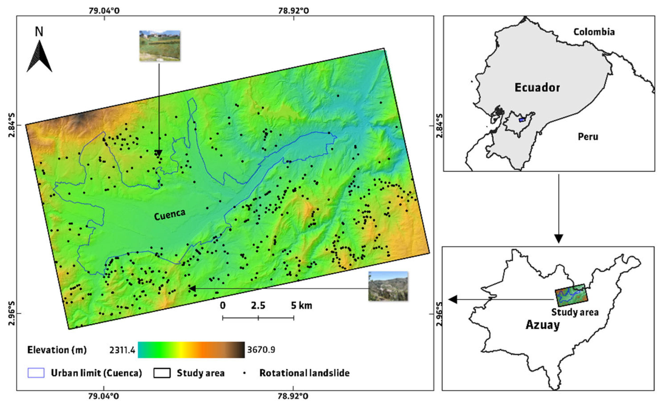
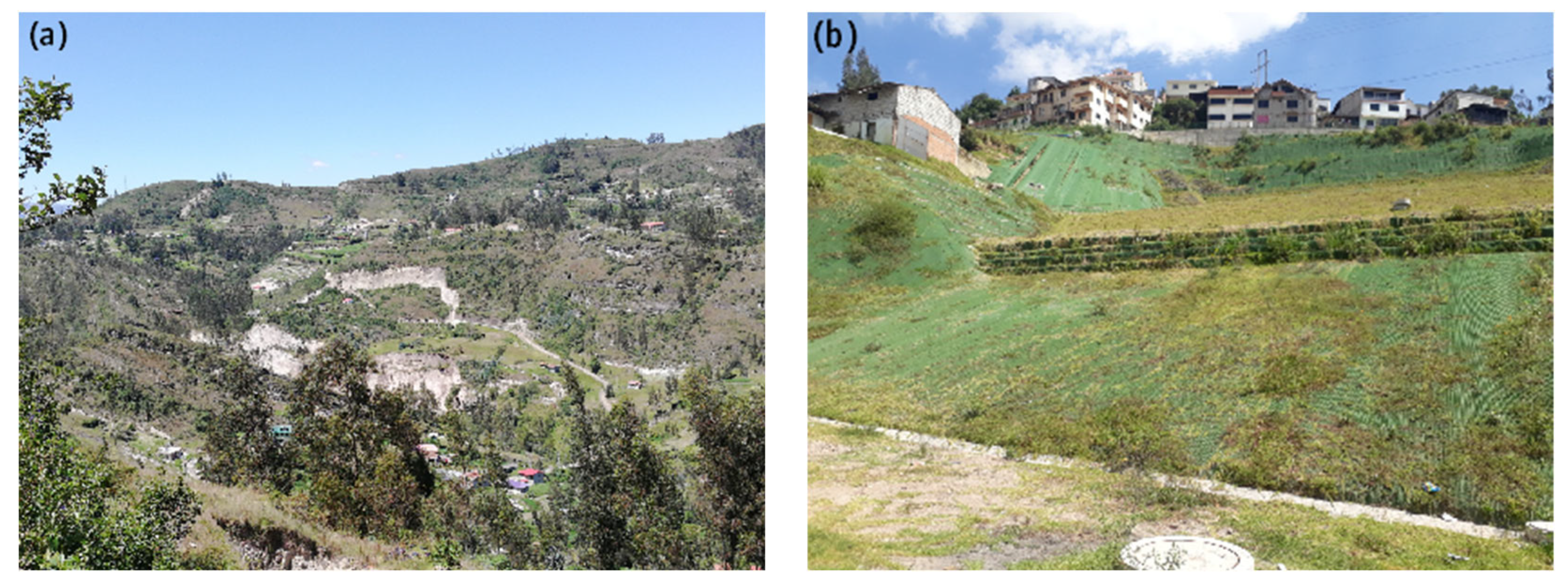
Study Area
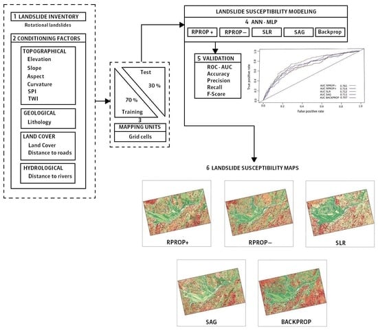
3. Methods
3.1. Obtaining the Landslide Inventory
3.2. Generation of Conditioning Factors
3.3. Extraction of Training and Test Datasets
3.4. Implementation of the ANN-MLP Algorithm
Hyperparameter Settings
3.5. Results Validation
3.6. Obtaining Landslide Susceptibility Maps (LSMs)
4. Results
4.1. Correlation Analysis between Conditioning Factors
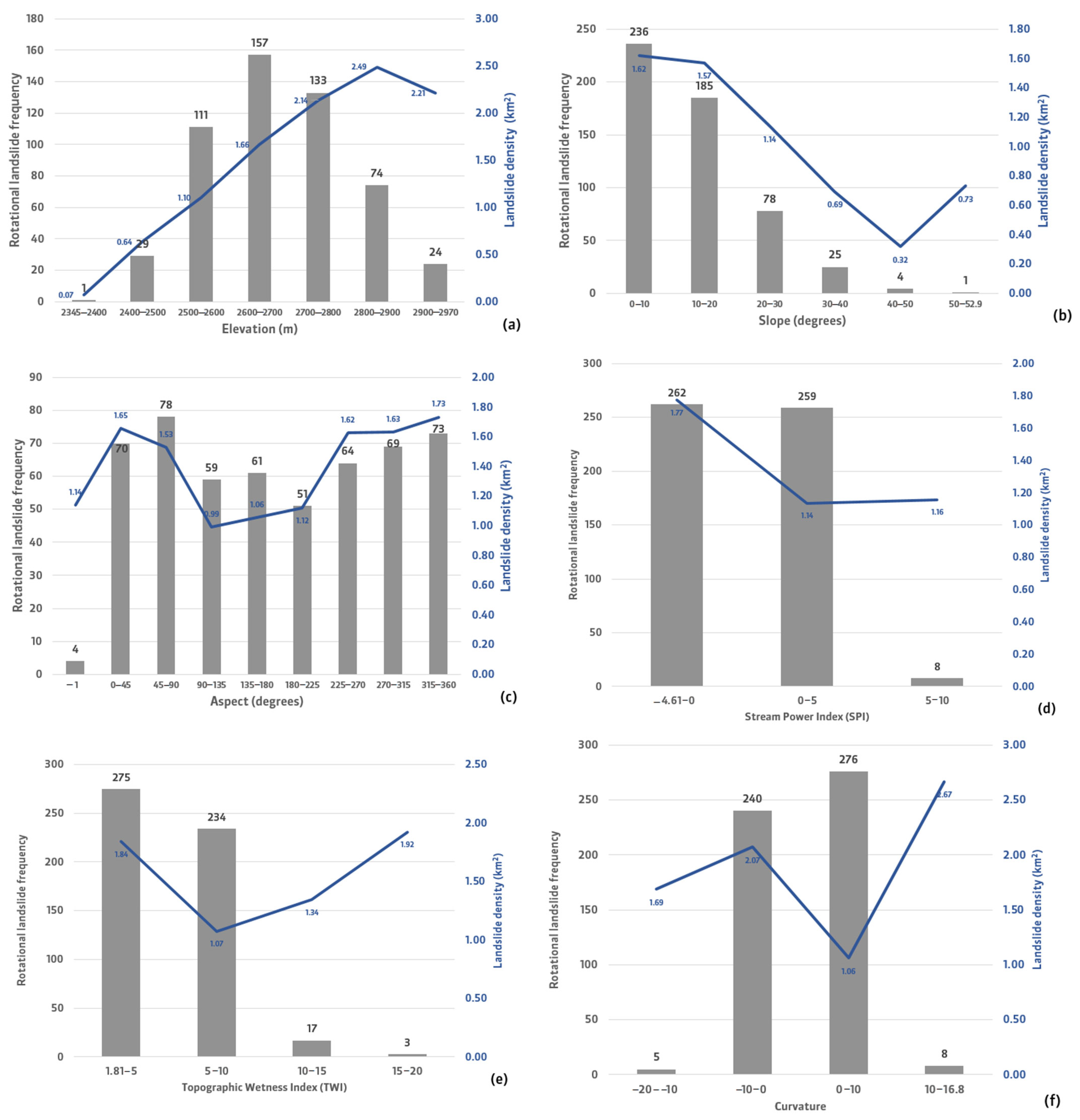
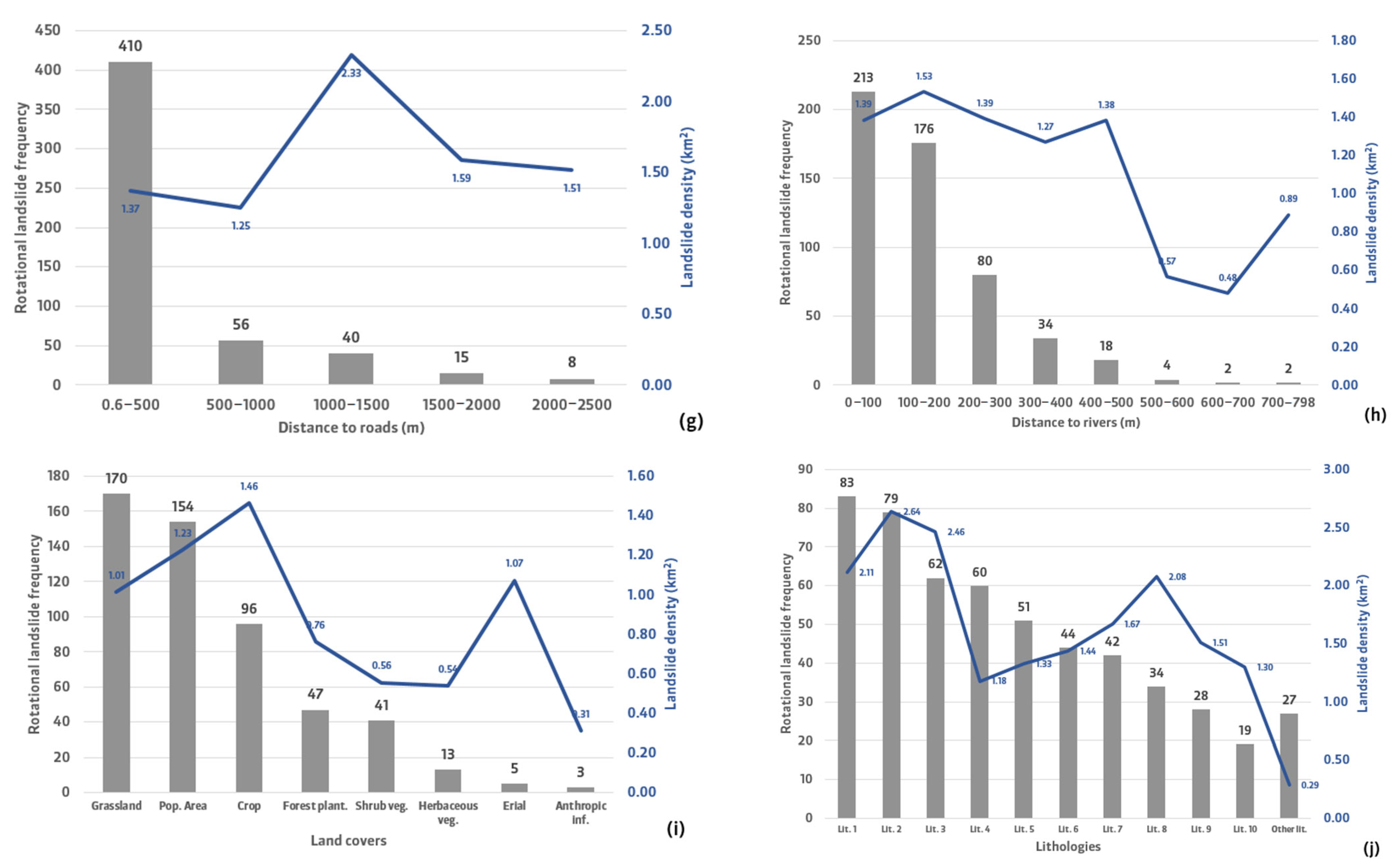
4.2. Landslide Analysis According to Conditioning Factors
4.3. ANN Implementation and Performance
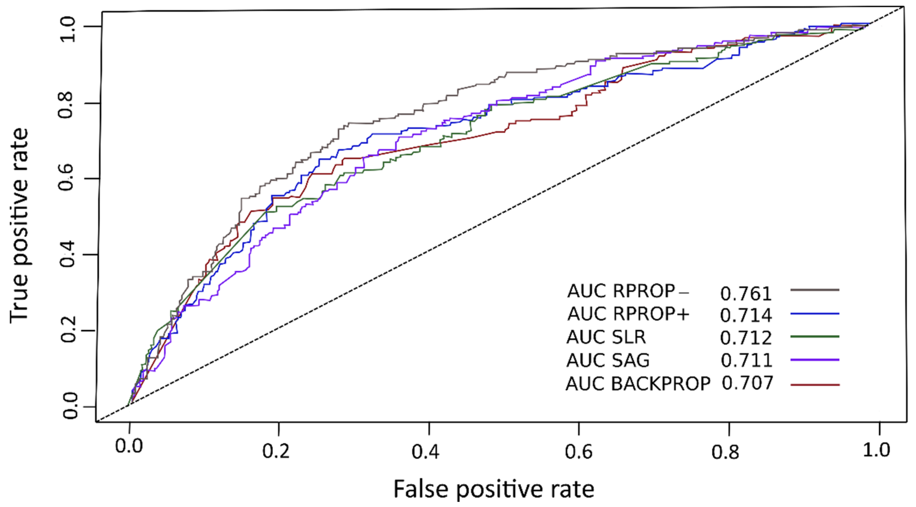
4.4. Results Validation
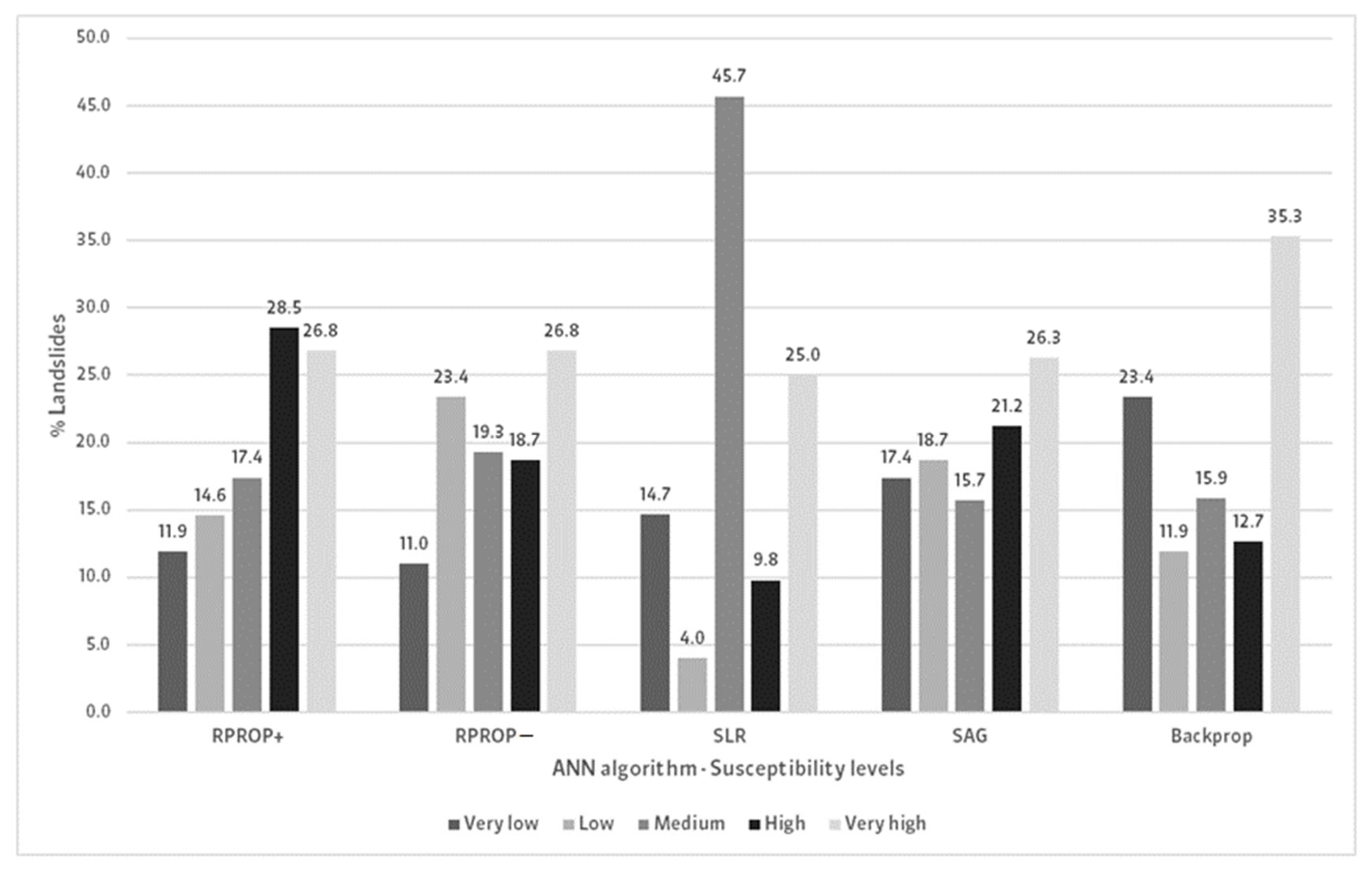
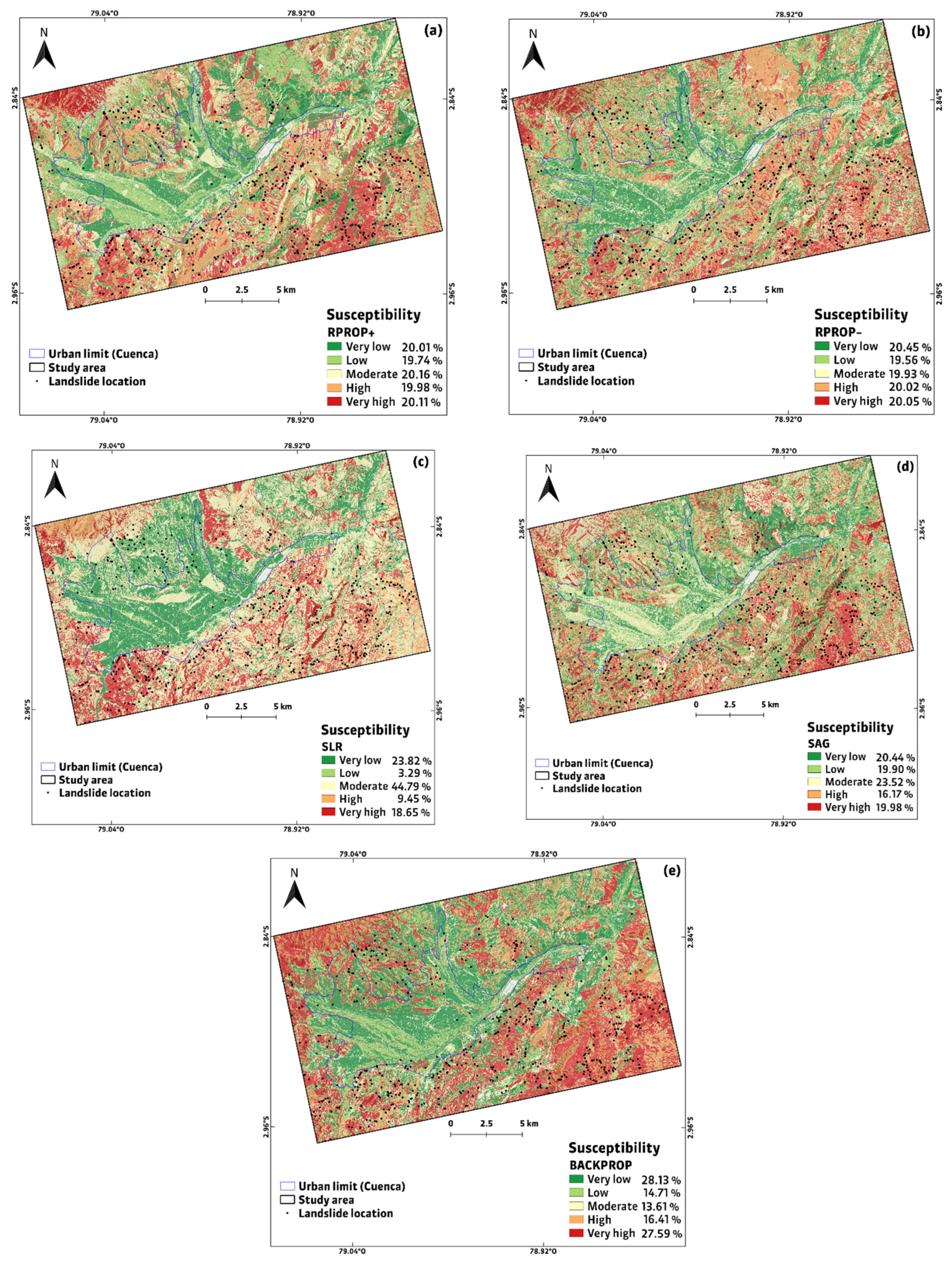
4.5. Landslide Susceptibility Analysis
5. Discussion
6. Conclusions
Author Contributions
Funding
Data Availability Statement
Acknowledgments
Conflicts of Interest
References
- Schuster, R.L. Socioeconomic Significance of Landslides. Spec. Rep.—Natl. Res. Counc. Transp. Res. Board 1996, 247, 12–35. [Google Scholar]
- Varnes, D.J. Landslide Hazard Zonation: A Review of Principles and Practice; United Nations, Education, Scientific and Cultural Organization, Ed.; United Nations: Paris, France, 1984. [Google Scholar]
- United Nations Office for Disaster Risk Reduction. Global Assessment Report on Disaster Risk Reduction 2019; United Nations Office for Disaster Risk Reduction: Geneva, Switzerland, 2019. [Google Scholar]
- (UNDRR)., U.N.O. for D.R.R. The Sendai Framework and the Sustainable Development Goals (SDG). Available online: https://www.undrr.org/implementing-sendai-framework/sf-and-sdgs (accessed on 6 April 2022).
- Fernández, T.; Jiménez, J.; Delgado, J.; Cardenal, J.; Pérez, J.L.; El Hamdouni, R.; Irigaray, C.; Chacón, J. Methodology for Landslide Susceptibility and Hazard Mapping Using GIS and SDI. In Intelligent Systems for Crisis Management; Lecture Notes in Geoinformation and Cartography; Springer: Berlin/Heidelberg, Germany, 2013. [Google Scholar]
- Conforti, M.; Pascale, S.; Robustelli, G.; Sdao, F. Evaluation of Prediction Capability of the Artificial Neural Networks for Mapping Landslide Susceptibility in the Turbolo River Catchment (Northern Calabria, Italy). Catena 2014, 113, 236–250. [Google Scholar] [CrossRef]
- Yilmaz, I. A Case Study from Koyulhisar (Sivas-Turkey) for Landslide Susceptibility Mapping by Artificial Neural Networks. Bull. Eng. Geol. Environ. 2009, 68, 297–306. [Google Scholar] [CrossRef]
- Bandara, A.; Hettiarachchi, Y.; Hettiarachchi, K.; Munasinghe, S.; Wijesinghe, I.; Thayasivam, U. A Generalized Ensemble Machine Learning Approach for Landslide Susceptibility Modeling. In Proceedings of the Advances in Intelligent Systems and Computing; Springer: Singapore, 2020; Volume 1016. [Google Scholar]
- Guzzetti, F.; Carrara, A.; Cardinali, M.; Reichenbach, P. Landslide Hazard Evaluation: A Review of Current Techniques and Their Application in a Multi-Scale Study, Central Italy. Geomorphology 1999, 31, 181–216. [Google Scholar] [CrossRef]
- Petley, D. Global Patterns of Loss of Life from Landslides. Geology 2012, 40, 927–930. [Google Scholar] [CrossRef]
- Hungr, O.; Leroueil, S.; Picarelli, L. The Varnes Classification of Landslide Types, an Update. Landslides 2014, 11, 167–194. [Google Scholar] [CrossRef]
- Varnes, D. Slope Movement Types and Processes. Spec. Rep. 1978, 176, 11–33. [Google Scholar]
- Corominas, J. Predicción de Movimientos de Ladera. Mapas de Susceptibilidad y Peligrosidad. In Riesgos Naturales Y Desarrollo Sostenible: Impacto, predicción y mitigación; Serie: Medio Ambiente; Riesgos Geológicos: Madrid; Ayala-Carcedo, F., Olcina-Cantos, J., Laín-Huerta, L., González-Jiménez, A., Eds.; Publicaciones del Instituto Geológico y Minero de España: Madrid, Spain, 2006; pp. 207–220. [Google Scholar]
- Highland, L.M.; Bobrowsky, P. The Landslide Handbook—A Guide to Understanding Landslides; US Geological Survey: Fairfax, VA, USA, 2008. [Google Scholar]
- Brabb, E. Innovative Approaches to Landslide Hazard and Risk Mapping. In Proceedings of the 4th International Symposium on Landslides, Toronto, ON, Canada, 16–21 September 1984; pp. 307–323. [Google Scholar]
- Di Napoli, M.; Carotenuto, F.; Cevasco, A.; Confuorto, P.; Di Martire, D.; Firpo, M.; Pepe, G.; Raso, E.; Calcaterra, D. Machine Learning Ensemble Modelling as a Tool to Improve Landslide Susceptibility Mapping Reliability. Landslides 2020, 17, 1897–1914. [Google Scholar] [CrossRef]
- Yu, C.; Chen, J. Landslide Susceptibility Mapping Using the Slope Unit for Southeastern Helong City, Jilin Province, China: A Comparison of ANN and SVM. Symmetry 2020, 12, 1047. [Google Scholar] [CrossRef]
- Sahin, E.K. Assessing the Predictive Capability of Ensemble Tree Methods for Landslide Susceptibility Mapping Using XGBoost, Gradient Boosting Machine, and Random Forest. SN Appl. Sci. 2020, 2, 1–17. [Google Scholar] [CrossRef]
- Carrara, A. Multivariate Models for Landslide Hazard Evaluation. J. Int. Assoc. Math. Geol. 1983, 15, 403–426. [Google Scholar] [CrossRef]
- Chung, C.J.F.; Fabbri, A.G. Probabilistic Prediction Models for Landslide Hazard Mapping. Photogramm. Eng. Remote Sens. 1999, 65, 1389–1399. [Google Scholar]
- Reichenbach, P.; Rossi, M.; Malamud, B.D.; Mihir, M.; Guzzetti, F. A Review of Statistically-Based Landslide Susceptibility Models. Earth-Sci. Rev. 2018, 180, 60–91. [Google Scholar] [CrossRef]
- Shano, L.; Raghuvanshi, T.K.; Meten, M. Landslide Susceptibility Evaluation and Hazard Zonation Techniques–a Review. Geoenvironmental Disasters 2020, 7, 1–19. [Google Scholar] [CrossRef]
- Van Westen, C.J. The Modeling of Landslide Hazards Using GIS. Surv. Geophys. 2000, 21, 241–255. [Google Scholar] [CrossRef]
- Deparday, V.; Gevaert, C.; Molinario, G.; Soden, R.; Balog-Way, S. Machine Learning for Disaster Risk Management; World Bank: Carroll, NH, USA, 2019. [Google Scholar]
- Pourghasemi, H.R.; Rahmati, O. Prediction of the Landslide Susceptibility: Which Algorithm, Which Precision? Catena 2018, 162, 177–192. [Google Scholar] [CrossRef]
- Dou, J.; Yamagishi, H.; Pourghasemi, H.R.; Yunus, A.P.; Song, X.; Xu, Y.; Zhu, Z. An Integrated Artificial Neural Network Model for the Landslide Susceptibility Assessment of Osado Island, Japan. Nat. Hazards 2015, 78, 1749–1776. [Google Scholar] [CrossRef]
- Huang, F.; Cao, Z.; Guo, J.; Jiang, S.H.; Li, S.; Guo, Z. Comparisons of Heuristic, General Statistical and Machine Learning Models for Landslide Susceptibility Prediction and Mapping. Catena 2020, 191, 104580. [Google Scholar] [CrossRef]
- Liu, Y.; Zhang, W.; Zhang, Z.; Xu, Q.; Li, W. Risk Factor Detection and Landslide Susceptibility Mapping Using Geo-Detector and Random Forest Models: The 2018 Hokkaido Eastern Iburi Earthquake. Remote Sens. 2021, 13, 1157. [Google Scholar] [CrossRef]
- Wang, Z.; Brenning, A. Active-learning Approaches for Landslide Mapping Using Support Vector Machines. Remote Sens. 2021, 13, 2588. [Google Scholar] [CrossRef]
- Abbaszadeh Shahri, A.; Spross, J.; Johansson, F.; Larsson, S. Landslide Susceptibility Hazard Map in Southwest Sweden Using Artificial Neural Network. Catena 2019, 183, 104225. [Google Scholar] [CrossRef]
- Harmouzi, H.; Nefeslioglu, H.A.; Rouai, M.; Sezer, E.A.; Dekayir, A.; Gokceoglu, C. Landslide Susceptibility Mapping of the Mediterranean Coastal Zone of Morocco between Oued Laou and El Jebha Using Artificial Neural Networks (ANN). Arab. J. Geosci. 2019, 12, 696. [Google Scholar] [CrossRef]
- Ortiz, J.A.V.; Martínez-Graña, A.M. A Neural Network Model Applied to Landslide Susceptibility Analysis (Capitanejo, Colombia). Geomat. Nat. Hazards Risk 2018, 9, 1106–1128. [Google Scholar] [CrossRef] [Green Version]
- Pham, B.T.; Tien Bui, D.; Prakash, I.; Dholakia, M.B. Hybrid Integration of Multilayer Perceptron Neural Networks and Machine Learning Ensembles for Landslide Susceptibility Assessment at Himalayan Area (India) Using GIS. Catena 2017, 149, 52–63. [Google Scholar] [CrossRef]
- Pradhan, B.; Lee, S. Regional Landslide Susceptibility Analysis Using Back-Propagation Neural Network Model at Cameron Highland, Malaysia. Landslides 2010, 7, 13–30. [Google Scholar] [CrossRef]
- Tien Bui, D.; Tuan, T.A.; Klempe, H.; Pradhan, B.; Revhaug, I. Spatial Prediction Models for Shallow Landslide Hazards: A Comparative Assessment of the Efficacy of Support Vector Machines, Artificial Neural Networks, Kernel Logistic Regression, and Logistic Model Tree. Landslides 2016, 13, 361–378. [Google Scholar] [CrossRef]
- Ghorbanzadeh, O.; Shahabi, H.; Crivellari, A.; Homayouni, S.; Blaschke, T.; Ghamisi, P. Landslide Detection Using Deep Learning and Object-Based Image Analysis. Landslides 2022, 19, 929–939. [Google Scholar] [CrossRef]
- Piralilou, S.T.; Shahabi, H.; Pazur, R. Automatic Landslide Detection Using Bi-Temporal Sentinel 2 Imagery. GI_Forum 2021, 1, 39–45. [Google Scholar] [CrossRef]
- Tang, X.; Tu, Z.; Wang, Y.; Liu, M.; Li, D.; Fan, X. Automatic Detection of Coseismic Landslides Using a New Transformer Method. Remote Sens. 2022, 14, 2884. [Google Scholar] [CrossRef]
- Ghorbanzadeh, O.; Blaschke, T.; Gholamnia, K.; Meena, S.R.; Tiede, D.; Aryal, J. Evaluation of Different Machine Learning Methods and Deep-Learning Convolutional Neural Networks for Landslide Detection. Remote Sens. 2019, 11, 196. [Google Scholar] [CrossRef] [Green Version]
- Di Napoli, M.; Annibali Corona, M.; Guerriero, L.; Miele, P.; Sellers, C.; Di Martire, D. Landslide Susceptibility Assessment in Expansion Areas of the Rapidly Growing City of Cuenca (Ecuador). Rend. Online Della Soc. Geol. Ital. 2022, 56, 50–54. [Google Scholar] [CrossRef]
- Lin, J.; He, P.; Yang, L.; He, X.; Lu, S.; Liu, D. Predicting Future Urban Waterlogging-Prone Areas by Coupling the Maximum Entropy and FLUS Model. Sustain. Cities Soc. 2022, 80, 103812. [Google Scholar] [CrossRef]
- Rahmati, O.; Golkarian, A.; Biggs, T.; Keesstra, S.; Mohammadi, F.; Daliakopoulos, I.N. Land Subsidence Hazard Modeling: Machine Learning to Identify Predictors and the Role of Human Activities. J. Environ. Manage. 2019, 236, 466–480. [Google Scholar] [CrossRef]
- Javidan, N.; Kavian, A.; Pourghasemi, H.R.; Conoscenti, C.; Jafarian, Z.; Rodrigo-Comino, J. Evaluation of Multi-Hazard Map Produced Using MaxEnt Machine Learning Technique. Sci. Rep. 2021, 11, 1–20. [Google Scholar] [CrossRef]
- Ghorbanzadeh, O.; Xu, Y.; Ghamisi, P.; Kopp, M.; Kreil, D. Landslide4Sense: Reference Benchmark Data and Deep Learning Models for Landslide Detection. arXiv 2022, arXiv:2206.00515. [Google Scholar]
- Chacón, J.; Irigaray, C.; Fernández, T.; El Hamdouni, R. Engineering Geology Maps: Landslides and Geographical Information Systems. Bull. Eng. Geol. Environ. 2006, 65, 341–411. [Google Scholar] [CrossRef]
- Irigaray, C.; Fernández, T.; El Hamdouni, R.; Chacón, J. Evaluation and Validation of Landslide-Susceptibility Maps Obtained by a GIS Matrix Method: Examples from the Betic Cordillera (Southern Spain). Nat. Hazards 2006, 41, 61–79. [Google Scholar] [CrossRef]
- Irigaray, C. Peligrosidad Asociada a Los Movimientos de Ladera; Presented at the class of Natural Risks; University of Jaen: Jaen, Spain, 2021. [Google Scholar]
- Remondo, J.; Soto, J.; González-Díez, A.; Díaz de Terán, J.R.; Cendrero, A. Human Impact on Geomorphic Processes and Hazards in Mountain Areas in Northern Spain. Geomorphology 2005, 66, 69–84. [Google Scholar] [CrossRef]
- Lin, Y.-P.; Chu, H.-J.; Wu, C.-F. Spatial Pattern Analysis of Landslide Using Landscape Metrics and Logistic Regression: A Case Study in Central Taiwan. Hydrol. Earth Syst. Sci. Discuss. 2010, 7, 3423–3451. [Google Scholar] [CrossRef]
- Achour, Y.; Pourghasemi, H.R. How Do Machine Learning Techniques Help in Increasing Accuracy of Landslide Susceptibility Maps? Geosci. Front. 2019, 11, 871–883. [Google Scholar] [CrossRef]
- Guzzetti, F.; Reichenbach, P.; Cardinali, M.; Galli, M.; Ardizzone, F. Probabilistic Landslide Hazard Assessment at the Basin Scale. Geomorphology 2005, 72, 272–299. [Google Scholar] [CrossRef]
- Basabe, P.; Almeida, E.; Ramón, P.; Zeas, R.; Alvarez, L. Avance En La Prevención de Desastres Naturales En La Cuenca Del Río Paute, Ecuador. Bull. Inst. fr. {é}tudes Andin. 1996, 25, 443–458. [Google Scholar]
- (UNDRR), U.N.O. for D.R.R. DesInventar. Available online: https://www.desinventar.net (accessed on 17 December 2021).
- UCLouvain. Centre for Research on the Epidemiology of Disasters. Emergency Events Database. Available online: https://www.emdat.be/ (accessed on 17 December 2021).
- Vorpahl, P.; Elsenbeer, H.; Märker, M.; Schröder, B. How Can Statistical Models Help to Determine Driving Factors of Landslides? Ecol. Modell. 2012, 239, 27–39. [Google Scholar] [CrossRef]
- Soto, J.; Galve, J.P.; Palenzuela, J.A.; Azañón, J.M.; Tamay, J.; Irigaray, C. A Multi-Method Approach for the Characterization of Landslides in an Intramontane Basin in the Andes (Loja, Ecuador). Landslides 2017, 14, 1929–1947. [Google Scholar] [CrossRef]
- Soeters, R.; van Westen, C.J. Slope Instability Recognition, Analysis and Zonation Landslides Investigation and Mitigation. Landslides Investig. Mitig. Transp. Res. Board Spec. Rep. 1996, 247, 129–177. [Google Scholar]
- Sellers, C.A.; Buján, S.; Miranda, D. MARLI: A Mobile Application for Regional Landslide Inventories in Ecuador. Landslides 2021, 18, 3963–3977. [Google Scholar] [CrossRef]
- Rossel, F.; Le Goulven, P.; Cadier, E. Areal Distribution of the Influence of ENSO on the Annual Rainfall in Ecuador. Rev. des Sci. l’Eau 1999, 12, 183–200. [Google Scholar] [CrossRef] [Green Version]
- Bristow, E. Guide to the Geology of the Cuenca Basin, Southern Ecuador; Ecuadorian Geological and Geophysical Society: Quito, Ecuador, 1973. [Google Scholar]
- Miele, P.; Di Napoli, M.; Guerriero, L.; Ramondini, M.; Sellers, C.; Annibali Corona, M.; Di Martire, D. Landslide Awareness System (Laws) to Increase the Resilience and Safety of Transport Infrastructure: The Case Study of Pan-American Highway (Cuenca–Ecuador). Remote Sens. 2021, 13, 1564. [Google Scholar] [CrossRef]
- Milillo, P.; Sacco, G.; Di Martire, D.; Hua, H. Neural Network Pattern Recognition Experiments Toward a Fully Automatic Detection of Anomalies in InSAR Time Series of Surface Deformation. Front. Earth Sci. 2022, 9, 728643. [Google Scholar] [CrossRef]
- Confuorto, P.; Medici, C.; Bianchini, S.; Del Soldato, M.; Rosi, A.; Segoni, S.; Casagli, N. Machine Learning for Defining the Probability of Sentinel-1 Based Deformation Trend Changes Occurrence. Remote Sens. 2022, 14, 1748. [Google Scholar] [CrossRef]
- Ferretti, A.; Prati, C.; Rocca, F. Permanent Scatterers in SAR Interferometry. IEEE Trans. Geosci. Remote Sens. 2001, 39, 8–20. [Google Scholar] [CrossRef]
- Novellino, A.; Cesarano, M.; Cappelletti, P.; Di Martire, D.; Di Napoli, M.; Ramondini, M.; Sowter, A.; Calcaterra, D. Slow-Moving Landslide Risk Assessment Combining Machine Learning and InSAR Techniques. Catena 2021, 203, 105317. [Google Scholar] [CrossRef]
- van Westen, C.J.; Castellanos, E.; Kuriakose, S.L. Spatial Data for Landslide Susceptibility, Hazard, and Vulnerability Assessment: An Overview. Eng. Geol. 2008, 102, 112–131. [Google Scholar] [CrossRef]
- Fernández, T.; Irigaray, C.; El Hamdouni, R.; Chacón, J. Methodology for Landslide Susceptibility Mapping by Means of a GIS. Application to the Contraviesa Area (Granada, Spain). Nat. Hazards 2003, 30, 297–308. [Google Scholar] [CrossRef]
- Keller, E.; Blodgett, R. Introducción a Los Deslizamientos de Tierra. In Riesgos Naturales; Pearson Educación: London, UK, 2004; pp. 151–161. [Google Scholar]
- Azañón, J.M.; Pérez-Peña, J.; Yesares, J.; Rodríguez-Peces, M.; Roldán, F.; Mateos, R.; Rodríguez-Fernández, J.; Delgado, J.; Pérez, J.; Azor, A.; et al. Metodología Para El Análisis de La Susceptibilidad Frente a Deslizamientos En El Parque Nacional de Sierra Nevada Mediante SIG. Proy. De Investig. En Parq. Nac. Convoc. 2008, 2011, 7–24. [Google Scholar]
- Pourghasemi, H.R.; Rossi, M. Landslide Susceptibility Modeling in a Landslide Prone Area in Mazandarn Province, North of Iran: A Comparison between GLM, GAM, MARS, and M-AHP Methods. Theor. Appl. Climatol. 2017, 130, 609–633. [Google Scholar] [CrossRef]
- Li, J.; Wang, W.; Han, Z.; Li, Y.; Chen, G. Exploring the Impact of Multitemporal DEM Data on the Susceptibility Mapping of Landslides. Appl. Sci. 2020, 10, 2518. [Google Scholar] [CrossRef] [Green Version]
- Costanzo, D.; Rotigliano, E.; Irigaray, C.; Jiménez-Perálvarez, J.D.; Chacón, J. Factors Selection in Landslide Susceptibility Modelling on Large Scale Following the Gis Matrix Method: Application to the River Beiro Basin (Spain). Nat. Hazards Earth Syst. Sci. 2012, 12, 327–340. [Google Scholar] [CrossRef]
- Mandal, S.; Mondal, S. Statistical Approaches for Landslide Susceptibility Assessment and Prediction; Springer: Cham, Switzerland, 2018. [Google Scholar]
- Ba, Q.; Chen, Y.; Deng, S.; Yang, J.; Li, H. A Comparison of Slope Units and Grid Cells as Mapping Units for Landslide Susceptibility Assessment. Earth Sci. Informatics 2018, 11, 373–388. [Google Scholar] [CrossRef]
- Hearn, G.J.; Hart, A.B. Landslide Susceptibility Mapping: A Practitioner’s View. Bull. Eng. Geol. Environ. 2019, 78, 5811–5826. [Google Scholar] [CrossRef]
- Pham, B.T.; Pradhan, B.; Tien Bui, D.; Prakash, I.; Dholakia, M.B. A Comparative Study of Different Machine Learning Methods for Landslide Susceptibility Assessment: A Case Study of Uttarakhand Area (India). Environ. Model. Softw. 2016, 84, 240–250. [Google Scholar] [CrossRef]
- Ciaburro, G.; Venkateswaran, B. Neural Network with R: Smart Models Using CNN, RNN, Deep Learning, and Artificial Intelligence Principles; Packt Publishing Ltd: Birmingham, UK, 2017; Volume 91. [Google Scholar]
- Chen, H.; Zeng, Z.; Tang, H. Landslide Deformation Prediction Based on Recurrent Neural Network. Neural Process. Lett. 2015, 41, 169–178. [Google Scholar] [CrossRef]
- Günther, F.; Fritsch, S. Neuralnet: Training of Neural Networks. R J. 2010, 2, 30–38. [Google Scholar] [CrossRef] [Green Version]
- Wang, Y.; Fang, Z.; Hong, H. Comparison of Convolutional Neural Networks for Landslide Susceptibility Mapping in Yanshan County, China. Sci. Total Environ. 2019, 666, 975–993. [Google Scholar] [CrossRef] [PubMed]
- Wang, Y.; Fang, Z.; Wang, M.; Peng, L.; Hong, H. Comparative Study of Landslide Susceptibility Mapping with Different Recurrent Neural Networks. Comput. Geosci. 2020, 138, 104445. [Google Scholar] [CrossRef]
- Zare, M.; Pourghasemi, H.R.; Vafakhah, M.; Pradhan, B. Landslide Susceptibility Mapping at Vaz Watershed (Iran) Using an Artificial Neural Network Model: A Comparison between Multilayer Perceptron (MLP) and Radial Basic Function (RBF) Algorithms. Arab. J. Geosci. 2013, 6, 2873–2888. [Google Scholar] [CrossRef]
- Riedmiller, M.; Braun, H. Direct Adaptive Method for Faster Backpropagation Learning: The RPROP Algorithm. In Proceedings of the 1993 IEEE International Conference on Neural Networks, San Francisco, CA, USA, 28 March–1 April 1993. [Google Scholar]
- Hornik, K.; Stinchcombe, M.; White, H. Multilayer Feedforward Networks Are Universal Approximators. Neural Networks 1989, 2, 359–366. [Google Scholar] [CrossRef]
- Masters, T. Practical Neural Networks Recipes in C++; Academic Press Professional, Inc.: Cambridge, MA, USA, 1993. [Google Scholar]
- Zhao, P.; Masoumi, Z.; Kalantari, M.; Aflaki, M.; Mansourian, A. A GIS-Based Landslide Susceptibility Mapping and Variable Importance Analysis Using Artificial Intelligent Training-Based Methods. Remote Sens. 2022, 14, 211. [Google Scholar] [CrossRef]
- Peng, Y.; Peng, Z.; Lan, T. Neural Network Based Inverse Kinematics Solution for 6-R Robot Implement Using R Package Neuralnet. In Proceedings of the 2021 5th International Conference on Robotics and Automation Sciences, ICRAS 2021, Wuhan, China, 11–13 June 2021; pp. 65–69. [Google Scholar]
- Chen, L.; Liu, T.; Tang, B.; Xiang, H.; Sheng, Q. Modelling Traffic Noise in a Wide Gradient Interval Using Artificial Neural Networks. Environ. Technol. 2020, 42, 3561–3571. [Google Scholar] [CrossRef]
- Merghadi, A.; Yunus, A.P.; Dou, J.; Whiteley, J.; ThaiPham, B.; Bui, D.T.; Avtar, R.; Abderrahmane, B. Machine Learning Methods for Landslide Susceptibility Studies: A Comparative Overview of Algorithm Performance. Earth-Sci. Rev. 2020, 207, 103225. [Google Scholar] [CrossRef]
- Fritsch, S.; Günther, F.; Wright, M. Neuralnet: Training of Neural Networks; R Package Version 1.44.2; 2019. Available online: https://cran.r-project.org/web/packages/neuralnet/index.html (accessed on 30 November 2021).
- Kuhn, M. Bookdown: The Caret Package. 2019. Available online: https://topepo.github.io/caret/ (accessed on 14 March 2022).
- Zhang, Z. Neural Networks: Further Insights into Error Function, Generalized Weights and Others. Ann. Transl. Med. 2016, 4, 300. [Google Scholar] [CrossRef] [Green Version]
- Lai, J.S.; Tsai, F. Improving GIS-Based Landslide Susceptibility Assessments with Multi-Temporal Remote Sensing and Machine Learning. Sensors 2019, 19, 3717. [Google Scholar] [CrossRef] [Green Version]
- Xiao, T.; Segoni, S.; Chen, L.; Yin, K.; Casagli, N. A Step beyond Landslide Susceptibility Maps: A Simple Method to Investigate and Explain the Different Outcomes Obtained by Different Approaches. Landslides 2020, 17, 627–640. [Google Scholar] [CrossRef] [Green Version]
- Pascale, S.; Parisi, S.; Mancini, A.; Schiattarella, M.; Conforti, M.; Sole, A.; Murgante, B.; Sdao, F. Landslide Susceptibility Mapping Using Artificial Neural Network in the Urban Area of Senise and San Costantino Albanese (Basilicata, Southern Italy). In Proceedings of the Lecture Notes in Computer Science (including subseries Lecture Notes in Artificial Intelligence and Lecture Notes in Bioinformatics), Ho Chi Minh City, Vietnam, 24–27 June 2013; Spinger: Berlin/Heidelberg, Germany, 2013. [Google Scholar]
- Wubalem, A.; Meten, M. Landslide Susceptibility Mapping Using Information Value and Logistic Regression Models in Goncha Siso Eneses Area, Northwestern Ethiopia. SN Appl. Sci. 2020, 2, 1–19. [Google Scholar] [CrossRef] [Green Version]
- Sing, T.; Sander, O.; Beerenwinkel, N.; Lengauer, T. ROCR: Visualizing Classifier Performance in R. Bioinformatics 2005, 21, 3940–3941. [Google Scholar] [CrossRef]
- Kuhn, M.; Wing, J.; Weston, S.; Williams, A.; Keefer, C.; Engelhardt, A.; Cooper, T.; Mayer, Z.; Kenkel, B.; Benesty, M.; et al. Caret: Classification and Regression Training; R Package Version 6.0-84, R Packag. version 6.0-79. 2018. Available online: https://cran.r-project.org/web/packages/caret/index.html (accessed on 12 February 2022).
- Keyport, R.N.; Oommen, T.; Martha, T.R.; Sajinkumar, K.S.; Gierke, J.S. A Comparative Analysis of Pixel- and Object-Based Detection of Landslides from Very High-Resolution Images. Int. J. Appl. Earth Obs. Geoinf. 2018, 64, 1–11. [Google Scholar] [CrossRef]
- QGIS Development Team. 16. Working with Raster Data. 16.1 Raster Properties Dialog. Available online: https://docs.qgis.org/3.22/en/docs/user_manual/working_with_raster/raster_properties.html (accessed on 8 April 2022).
- Tien Bui, D.; Ho, T.C.; Pradhan, B.; Pham, B.T.; Nhu, V.H.; Revhaug, I. GIS-Based Modeling of Rainfall-Induced Landslides Using Data Mining-Based Functional Trees Classifier with AdaBoost, Bagging, and MultiBoost Ensemble Frameworks. Environ. Earth Sci. 2016, 75, 1–22. [Google Scholar] [CrossRef]
- Martín, B.; Alonso, J.C.; Martín, C.A.; Palacín, C.; Magaña, M.; Alonso, J. Influence of Spatial Heterogeneity and Temporal Variability in Habitat Selection: A Case Study on a Great Bustard Metapopulation. Ecol. Modell. 2012, 228, 39–48. [Google Scholar] [CrossRef]
- Ercanoglu, M.; Gokceoglu, C. Assessment of Landslide Susceptibility for a Landslide-Prone Area (North of Yenice, NW Turkey) by Fuzzy Approach. Environ. Geol. 2002, 41, 720–730. [Google Scholar] [CrossRef]
- Dou, J.; Yamagishi, H.; Xu, Y.; Zhu, Z.; Yunus, A.P. Characteristics of the Torrential Rainfall-Induced Shallow Landslides By Typhoon Bilis, in July 2006, Using Remote Sensing and GIS. In GIS Landslide; Springer: Berlin/Heidelberg, Germany, 2017; pp. 221–230. [Google Scholar]
- QGIS Development Team. 15. Working with Vector Data. 15.1 The Vector Properties Dialog. Available online: https://docs.qgis.org/3.22/en/docs/user_manual/working_with_vector/vector_properties.html (accessed on 24 February 2022).
- Chen, Z.; Ye, F.; Fu, W.; Ke, Y.; Hong, H. The Influence of DEM Spatial Resolution on Landslide Susceptibility Mapping in the Baxie River Basin, NW China. Nat. Hazards 2020, 101, 853–877. [Google Scholar] [CrossRef]
- Tian, Y.; Xiao, C.; Liu, Y.; Wu, L. Effects of Raster Resolution on Landslide Susceptibility Mapping: A Case Study of Shenzhen. Sci. China Ser. E Technol. Sci. 2008, 51, 188–198. [Google Scholar] [CrossRef]
- Baeza, C.; Lantada, N.; Amorim, S. Statistical and Spatial Analysis of Landslide Susceptibility Maps with Different Classification Systems. Environ. Earth Sci. 2016, 75, 1318. [Google Scholar] [CrossRef] [Green Version]
- González-Jiménez, A.; Carrasco, R.; Ayala-Carcedo, F.; de Pedraza, J.; Martín-Duque, J.; Sanz, M.; Bodoque, J. El Análisis de Susceptibilidad En La Prevención de Los Movimientos de Ladera: Un Análisis Comparativo de Las Metodologías Aplicadas En El Valle Del Jerte (Sistema Central Español). In Riesgos Naturales Y Desarrollo Sostenible: Impacto, Predicción Y Mitigación.; Ayala-Carcedo, F., Olcina-Cantos, J., Laín-Huerta, L., González-Jiménez, A., Eds.; Instituto Geológico y Minero de España: Madrid, Spain, 2006; pp. 221–246. [Google Scholar]


| Information | Element/Process Obtained | Source | Scale/Resolution |
|---|---|---|---|
| Satellite images and orthophotos for landslide inventory | Photo interpretation | Planet | 5 m |
| Ortophoto | 30 cm | ||
| DInSAR | Copernicus-Sentinel 1 | 5 × 20 m | |
| COSMO-SkyMed | 1 m | ||
| Landslide inventory | Rotational landslides | IERSE | - |
| Digital elevation model (DEM): Topographical maps | Aspect, curvature, elevation, slope, SPI, TWI | SIGTIERRAS-IERSE | 3 m |
| Geological map | Lithology | SNI | 1:100,000 |
| Soil cover: Land cover map Road layer | Land cover | SIGTIERRAS | 1:25,000 |
| Distance to roads | IGM | ||
| Hydrological: River layer | Distance to rivers | IGM | 1:25,000 |
| Global Factor | Conditioning Factor | Data Range (Unit) |
|---|---|---|
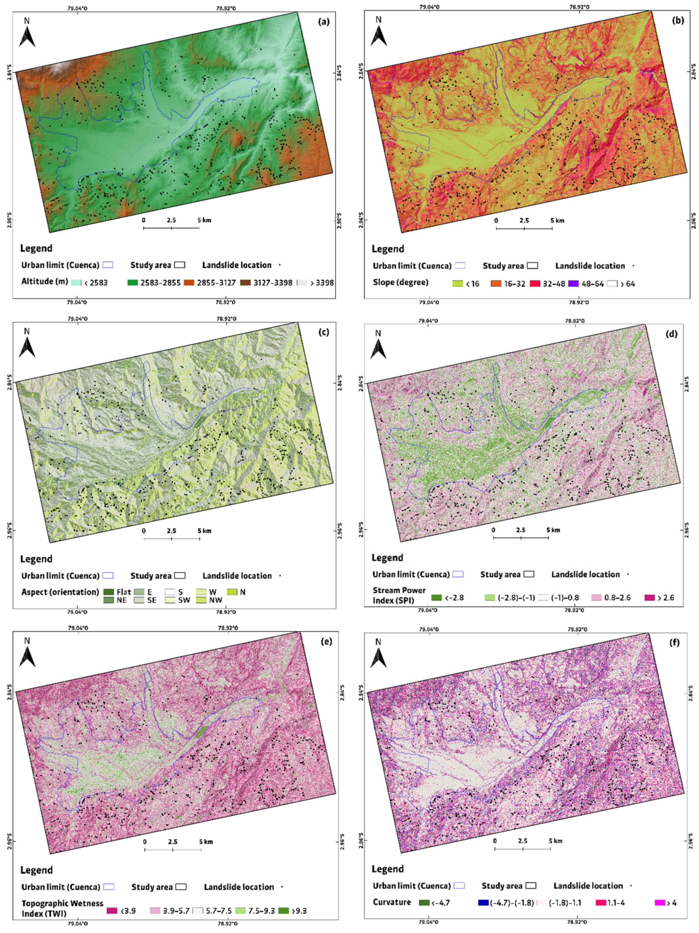
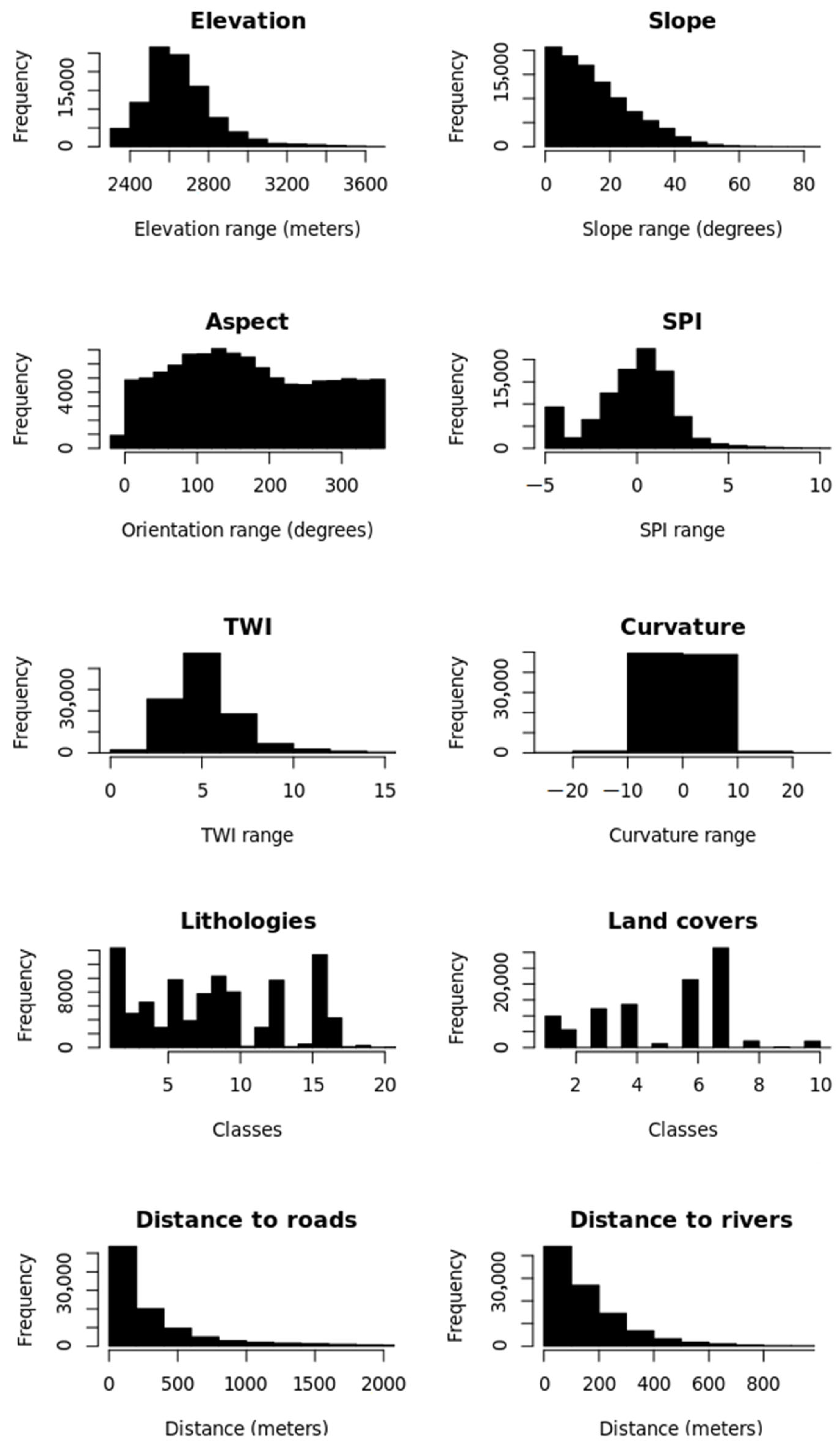
| Topographical | Elevation | (i) <2583, (ii) 2583–2855, (iii) 2855–3127, (iv) 3127–3398, (v) >3398 (m). |
| Slope | (i) <16, (ii) 16–32, (iii) 32–48, (iv) 48–64, (v) >64 (degree). | |
| Aspect | Flat zones −1°. 0°–22.5°(N); 22.5°–67.5° (NE); 67.5°–112.5° (E); 112.5°–157.5° (SE); 157.5°–202.5° (S); 202.5°–247.5° (SW); 247.5°–292.5° (W); 292.5°–337.5° (NW); 337.5°–360° (N). | |
| SPI | (i) <−2.8, (ii) −2.8–−1, (iii) −1–0.8, (iv) 0.8–2.6, (v) >2.6. | |
| TWI | (i) <3.9, (ii) 3.9–5.7, (iii) 5.7–7.5, (iv) 7.5–9.3, (v) >9.3. | |
| Curvature | (i) < −4.7, (ii) −4.7–−1.8, (iii) −1.8–1.1, (iv) 1.1–4 (v) >4. | |
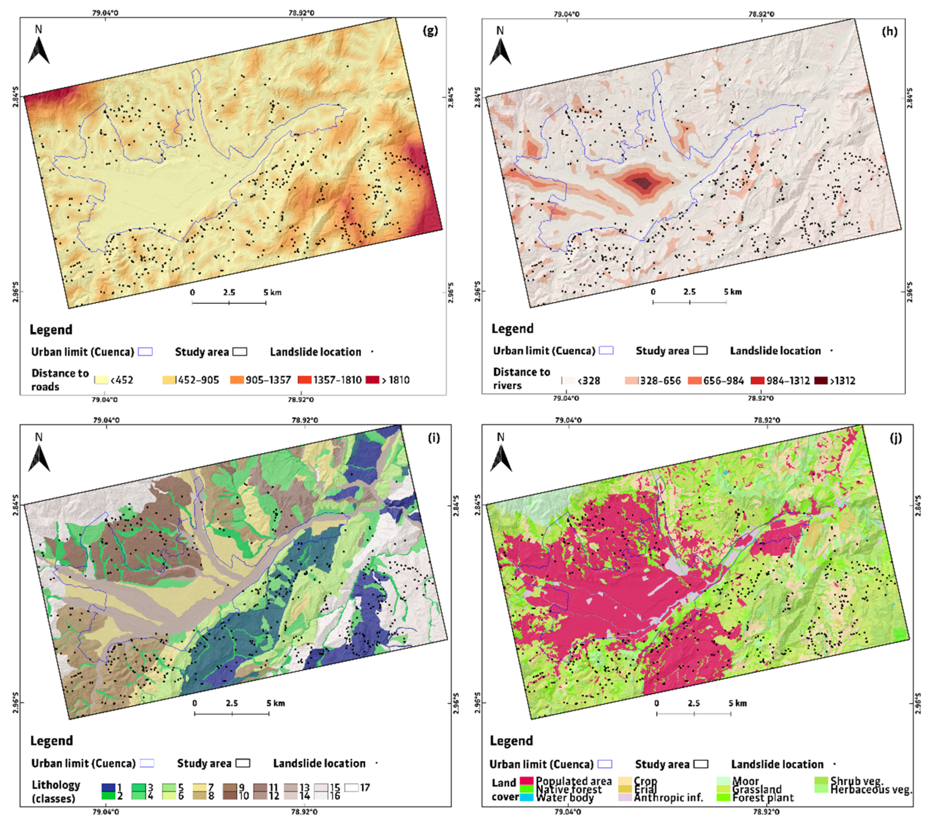
| Geological | Lithology | Principally 17: sandy clays; light laminated shales with gypsum; silts, clays, sands, gravels, and blocks; heterogeneous mixture of fine materials and fine angular fragments without stratification; heterogeneous mixture of fine materials and fine angular fragments (various sizes); medium to coarse-grained tobaceous sandstones; siltstones, shales and fine-grained sandstones; sandy silt, silty clay; coarse andesitic conglomerates; silts and clays; red clays with sandstones and conglomerates alternation; volcanic agglomerate; sands, silts, clays, and conglomerates; laminated mudstones, dark tobaceous sandstones; variable proportion of silts, clays, sands, gravels, and blocks; tuffs and agglomerates; massive siltstones. |
| Soil covers | Land cover | A total of 1903 coverages classified in 11 classes: forest plantation, grassland, populated area, shrub vegetation, herbaceous vegetation, crop, anthropic infrastructure, wasteland, water body, moorland, and native forest. |
| Distance to roads | (i) <452, (ii) 452–905, (iii) 905–1357, (iv) 1357–1810, (v) >1810 (m). | |
| Hydrological | Distance to rivers | (i) <328, (ii) 328–656, (iii) 656–984, (iv) 984–1312, (v) >1.312 (m). |
| Global Factor | Conditioning Factor | Relevance |
|---|---|---|
| Topographical | Elevation | The probability of landslide occurrence is larger in areas where the elevation is higher [71]. |
| Slope | Increasing slope decreases stability [55]. Its angle is considered as a controlling factor in landslide modeling [72]. | |
| Aspect | Indicates exposure to local climatic conditions [55] and atmospheric processes such as rainfall, wind, and solar radiation [73]. | |
| Curvature | Refers to a change in the slope gradient or aspect in a given direction [6]. Affects the control of water flow [33]. | |
| Stream power index (SPI) | Indicator of erosive processes caused by surface runoff. High SPI values indicate proximity to a stream. With low SPI values, a low susceptibility to landslide initiation is expected [55]. | |
| Topographic wetness index (TWI) | Indicator of saturated soil conditions during rainfall and sediment accumulation [55]. With a higher value of TWI, there is a greater tendency for the saturation of slope materials [73]. | |
| Geological | Lithology | Defines material where landslides occur [31] and influences geomechanical characteristics of terrain [72]. |
| Soil covers | Land cover | Each cover has characteristics and textures that influence landslide generation. It is also related to the degree of vegetation cover that influences the stability of slope materials [33]. |
| Distance to roads | Related to the process of road construction, which, when developed in mountainous areas, causes impacts on slope stability [25]. | |
| Hydrological | Distance to rivers | The closer this distance, the greater the probability of landslides [74]. It should be considered that a stream may be where landslides move to, which generates additional risk [75]. |
| Hyperparameter | Description | Setting Value |
|---|---|---|
| act.fct | Differentiable activation function [79] (no configuration was required in this research). | logistic (per default) |
| algorithm | Define algorithm to be implemented. | RPROP+, RPROP−, SLR, SAG, backprop |
| err.fct | Define the error function [92]. Used for the error calculation. | ce (cross entropy) |
| hidden | Define the number of hidden layers and neurons [79]. | 3 (one hidden layer with three neurons) |
| linear.output | If act.fct is not set, its default value is TRUE [79]. Change to FALSE for classification models. | FALSE |
| learningrate | Learning rate [79]. Applies only when algorithm = backprop. | 0.01 |
| stepmax | Define the maximum number of steps for ANN training [90]. | 1e + 8 |
| Aspect | Curvature | Elevation | Dist. Rivers | Dist. Roads | Land Cover | Lithology | Slope | SPI | TWI | |
|---|---|---|---|---|---|---|---|---|---|---|
| Aspect | 1 | |||||||||
| Curvature | 0.00 * | 1 | ||||||||
| Elevation | 0.02 | 0.03 | 1 | |||||||
| Dist. rivers | −0.02 | 0.04 | 0.17 | 1 | ||||||
| Dist. roads | 0.11 | 0.01 | 0.28 | −0.21 | 1 | |||||
| Land cover | −0.10 | −0.01 | −0.06 | 0.18 | −0.37 | 1 | ||||
| Lithology | −0.05 | 0.02 | 0.29 | 0.05 | 0.09 | 0.06 | 1 | |||
| Slope | 0.11 | 0.02 | 0.25 | −0.17 | 0.43 | −0.41 | 0.05 | 1 | ||
| SPI | 0.07 | −0.33 | 0.15 | −0.09 | 0.25 | −0.22 | 0.01 | 0.52 | 1 | |
| TWI | −0.09 | −0.34 | −0.15 | 0.10 | −0.22 | 0.24 | −0.02 | −0.56 | 0.33 | 1 |
| Algorithm | Runtime (Seconds) | Runtime (Minutes) |
|---|---|---|
| RPROP+ | 7.1 | ~0.12 |
| RPROP− | 6.9 | ~0.12 |
| SLR | 70.7 | ~1.18 |
| SAG | 9.8 | ~0.16 |
| Backprop | 560.7 | ~9.35 |
| Algorithm | AUC (Training) | AUC (Testing) |
|---|---|---|
| RPROP+ | 0.881 | 0.714 |
| RPROP− | 0.888 | 0.761 |
| SLR | 0.870 | 0.712 |
| SAG | 0.889 | 0.711 |
| Backprop | 0.867 | 0.707 |
| Algorithm | Training | |||
|---|---|---|---|---|
| Sens | Accuracy | PPV | F-Score | |
| RPROP+ | 0.887 | 0.837 | 0.900 | 0.894 |
| RPROP− | 0.873 | 0.850 | 0.940 | 0.905 |
| SLR | 0.812 | 0.820 | 0.996 | 0.894 |
| SAG | 0.853 | 0.844 | 0.961 | 0.904 |
| Backprop | 0.946 | 0.837 | 0.834 | 0.887 |
| Algorithm | Testing | |||
|---|---|---|---|---|
| Sens | Accuracy | PPV | F-Score | |
| RPROP+ | 0.832 | 0.748 | 0.839 | 0.836 |
| RPROP− | 0.815 | 0.764 | 0.894 | 0.853 |
| SLR | 0.789 | 0.775 | 0.964 | 0.868 |
| SAG | 0.800 | 0.754 | 0.905 | 0.849 |
| Backprop | 0.846 | 0.721 | 0.776 | 0.809 |
| LSM (RPROP+) | |||
|---|---|---|---|
| Susceptibility | Pixel Amount | Pixels (%) | Landslides (%) |
| Very low | 8,406,238 | 20.01 | 11.9 |
| Low | 8,294,697 | 19.74 | 14.6 |
| Medium | 8,468,934 | 20.16 | 17.4 |
| High | 8,396,090 | 19.98 | 28.5 |
| Very high | 8,449,935 | 20.11 | 26.8 |
| LSM (RPROP−) | |||
| Susceptibility | Pixel amount | Pixels (%) | Landslides (%) |
| Very low | 8,590,183 | 20.45 | 11.0 |
| Low | 8,217,572 | 19.56 | 23.4 |
| Medium | 8,374,349 | 19.93 | 19.3 |
| High | 8,410,428 | 20.02 | 18.7 |
| Very high | 8,423,362 | 20.05 | 26.8 |
| LSM (SLR) | |||
| Susceptibility | Pixel amount | Pixels (%) | Landslides (%) |
| Very low | 10,007,252 | 23.82 | 14.7 |
| Low | 1,383,762 | 3.29 | 4.0 |
| Medium | 18,820,629 | 44.79 | 45.7 |
| High | 3,968,797 | 9.45 | 9.8 |
| Very high | 7,835,454 | 18.65 | 25.0 |
| LSM (SAG) | |||
| Susceptibility | Pixel amount | Pixels (%) | Landslides (%) |
| Very low | 8,585,964 | 20.44 | 17.4 |
| Low | 8,360,306 | 19.90 | 18.7 |
| Medium | 9,881,636 | 23.52 | 15.7 |
| High | 6,792,878 | 16.17 | 21.2 |
| Very high | 8,395,110 | 19.98 | 26.3 |
| LSM (Backprop) | |||
| Susceptibility | Pixel amount | Pixels (%) | Landslides (%) |
| Very low | 11,818,586 | 28.13 | 23.4 |
| Low | 6,182,545 | 14.71 | 11.9 |
| Medium | 5,528,573 | 13.16 | 15.9 |
| High | 6,894,785 | 16.41 | 12.7 |
| Very high | 11,591,405 | 27.59 | 35.3 |
Publisher’s Note: MDPI stays neutral with regard to jurisdictional claims in published maps and institutional affiliations. |
© 2022 by the authors. Licensee MDPI, Basel, Switzerland. This article is an open access article distributed under the terms and conditions of the Creative Commons Attribution (CC BY) license (https://creativecommons.org/licenses/by/4.0/).
Share and Cite
Bravo-López, E.; Fernández Del Castillo, T.; Sellers, C.; Delgado-García, J. Landslide Susceptibility Mapping of Landslides with Artificial Neural Networks: Multi-Approach Analysis of Backpropagation Algorithm Applying the Neuralnet Package in Cuenca, Ecuador. Remote Sens. 2022, 14, 3495. https://doi.org/10.3390/rs14143495
Bravo-López E, Fernández Del Castillo T, Sellers C, Delgado-García J. Landslide Susceptibility Mapping of Landslides with Artificial Neural Networks: Multi-Approach Analysis of Backpropagation Algorithm Applying the Neuralnet Package in Cuenca, Ecuador. Remote Sensing. 2022; 14(14):3495. https://doi.org/10.3390/rs14143495
Chicago/Turabian StyleBravo-López, Esteban, Tomás Fernández Del Castillo, Chester Sellers, and Jorge Delgado-García. 2022. "Landslide Susceptibility Mapping of Landslides with Artificial Neural Networks: Multi-Approach Analysis of Backpropagation Algorithm Applying the Neuralnet Package in Cuenca, Ecuador" Remote Sensing 14, no. 14: 3495. https://doi.org/10.3390/rs14143495
APA StyleBravo-López, E., Fernández Del Castillo, T., Sellers, C., & Delgado-García, J. (2022). Landslide Susceptibility Mapping of Landslides with Artificial Neural Networks: Multi-Approach Analysis of Backpropagation Algorithm Applying the Neuralnet Package in Cuenca, Ecuador. Remote Sensing, 14(14), 3495. https://doi.org/10.3390/rs14143495