Estimation of Seaweed Biomass Based on Multispectral UAV in the Intertidal Zone of Gouqi Island

Abstract

UAV remote sensing inversion is an efficient and accurate method for obtaining information on vegetation coverage, biomass and other parameters. It is widely used on forest, grassland and other terrestrial vegetation. However, it is rarely used on aquatic vegetation, especially in intertidal zones and other complex environments. Additionally, it is mainly used for inversion of coverage, and there have been few studies thus far on biomass assessment. In this paper, we applied multispectral UAV aerial photography data to evaluate the biomass of seaweed in an intertidal zone. During the ebb tide, UAV aerial photography and in situ sampling data were collected in the study area. After optimizing the spectral index and performing a multiple linearity test, the spectral parameters were selected as the input of the evaluation model. Combined with two machine learning algorithms, namely random forest (RF) and gradient boosting decision tree (GBDT), the biomasses of three species of seaweed (Ulva pertusa, Sargassum thunbergii and Sargassum fusiforme) in the intertidal zone were assessed. In addition, the input parameters of the machine learning algorithms were optimized by one-way ANOVA and Pearson’s correlation analysis. We propose a method to assess the biomass of intertidal seaweed based on multispectral UAV data combined with statistics and machine learning. The results show that the two machine learning algorithms have different accuracies in terms of biomass evaluation using multispectral images; the gradient boosting decision tree can evaluate the biomass of seaweed in the intertidal zone more accurately.

1. Introduction

Seaweed, as a supporting organism of nearshore ecosystems, plays an important role in both the conservation of fishery resources and improving water quality [1]. Globally, seaweed widely inhabits 25% of the intertidal coastline [2], providing a steady stream of primary productivity to the coastal ecosystem. It is a fundamental component of nearshore habitat protection and marine blue carbon sinks [3]. In addition, seaweed can also be used as feed, in pharmaceuticals and as a fertilizer [4,5,6]. However, due to human activities and climate change, global warming and ocean acidification are increasing, and the degradation of seaweed in the intertidal zone is a serious issue [7]. Therefore, it is urgent to protect, repair and sensibly develop seaweed resources. The above ground biomass of seaweed is the basic parameter for the rational development and utilization of marine resources, the calculation of total nearshore carbon sinks and the evaluation of offshore ecosystem restoration effects [8]. At present, investigation and research on seaweed biomass are mainly carried out by quadrat sampling. The spatial scope of such investigations is very limited, so it is difficult to evaluate the status of seaweed resources on a large scale [9].

As efficient monitoring methods, satellite and UAV remote sensing technologies are continuously combined with water quality prediction and offshore ecological research, promoting large-scale offshore habitat research. They can also enable efficient, accurate and large-scale dynamic monitoring of a given study area [10,11,12,13]. At present, wild seaweed and cultured seaweed are often monitored. UAV is being increasingly used in vegetation ecology [14,15]. For the monitoring and research of cultured seaweed, due to its wide coverage and strong homogeneity, identification and analysis can be achieved by using satellite remote sensing technology [16]. In areas where the intertidal zone is wide, this technology can also monitor and study the distribution of seaweed [17,18,19]. However, for narrow intertidal zones, if we want to carry out more detailed research regarding the distribution range, species identification and biomass estimation, the monitoring accuracy of medium-resolution satellite remote sensing technology is not ideal. At present, the most common surveying method used for intertidal seaweed is an in situ quadrat sampling survey [9,20,21]. Therefore, it is very important to carry out high-precision seaweed surveys in typical narrow intertidal zones through UAV equipped with various sensors. This has broad application prospects. In addition, UAV remote sensing is more suitable for the high-precision quantitative monitoring of biological parameters, such as biomass [22,23,24]. Multispectral sensors carried by light multi-rotor UAV have attracted extensive attention in the field of agricultural quantitative remote sensing due to their low cost and multi-band nature (including the red edge band for vegetation monitoring) [25].

In this article, taking Gouqi Island, Shengsi County, Zhejiang Province, China, as an example, we analyze multiple spectral parameters of three species of seaweed in the intertidal zone by using the multi-spectral UAV survey method, and the spectral index is optimized using the near-infrared band. At the same time, in order to explore the optimal method and inversion accuracy of seaweed biomass calculated from UAV multispectral data, two machine learning methods, gradient boosting decision tree (GBDT) and random forest (RF), are compared. GBDT has been applied in many fields such as power engineering, transportation and control engineering [26,27,28,29], but there are no relevant reports on the prediction of seaweed biomass in an intertidal zone. As classical algorithms of regression and classification, SVM and RF are widely used in the quantitative inversion of grassland and forest biomass [30,31,32,33]. In recent years, they have also been applied in fishery remote sensing [34]. By comparing the regression and machine learning methods, we hope to provide an optimal solution for the accurate estimation of nearshore seaweed resources.

2. Materials and Methods

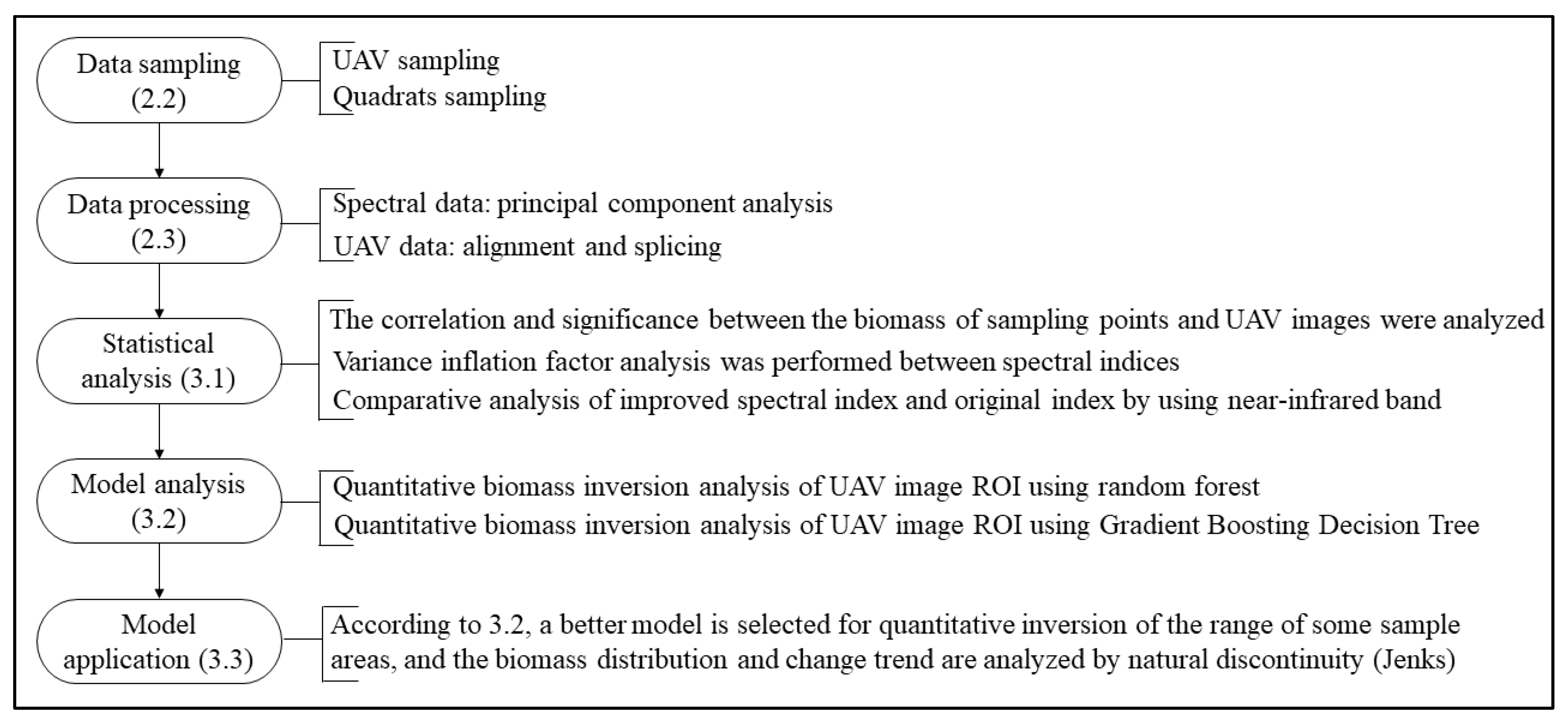
This work includes seven investigation phases (Figure 1): (i) multispectral UAV image acquisition; (ii) biomass, slope and GPS acquisition based on 0.25 × 0.25 m quadrats; (iii) multispectral image registration and stitching preprocessing; (iv) extraction of the region of interest (ROI) according to the quadrats’ size and position; (v) spectral analysis based on the ROI; (vi) seaweed biomass assessment based on a machine learning algorithm; and (vii) the application of an optimal model.

2.1. Study Area

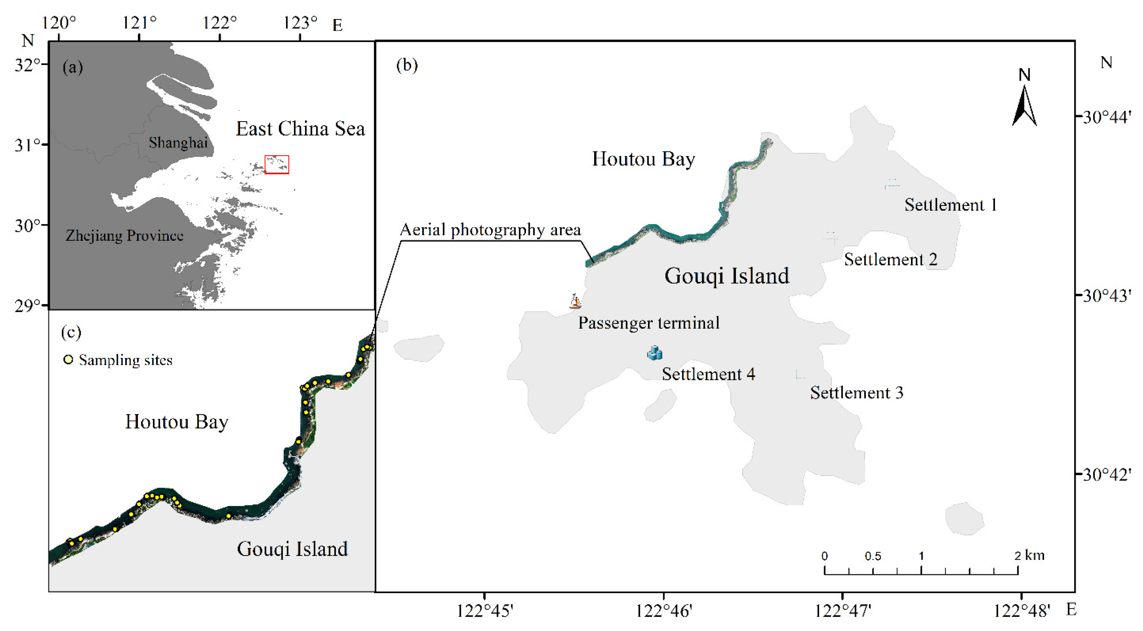
Gouqi Island (30°43′1.64″N, 122°46′3.25″E) is located in the south of the Ma’an islands in Shengsi County, Zhejiang Province, China. There are many islands and reefs in the nearby sea area, and rich biological resources. It has a unique natural landform of islands and reefs, and has biodiversity characteristics of an intertidal zone. The nearshore sediment is mainly composed of rocks and reefs, where many seaweeds grow, live and multiply, forming a complex nearshore marine ecosystem [35]. Seaweed in Gouqi island is the most prosperous in the summer and autumn. The investigation time of this study was 11:30–13:30 (UTC/GMT +08:00) on 17–24 June 2021. In order to highlight the actual growth and supply of seaweed in Gouqi Island, the nearshore of Houtou Bay, which is far from human influence and is representative of the survey site, was selected as the area for UAV aerial photography and field sample collection (Figure 2).

2.2. Sampling Method

On 25 June 2021, a DJI M300 RTK four-wing multicopter UAV (Dà-Jiāng Innovations Science and Technology Co., Ltd., Shenzhen, China) and MS600pro multispectral camera (Dà-Jiāng Innovations Science and Technology Co., Ltd., Shenzhen, China) (Figure 3) were used to collect multispectral images at 11:00–13:00 (UTC/GMT +08:00) on a clear and cloudless noon. At the time of sampling, the tide was the lowest of the flood season. Before each flight, the sensors were calibrated by a Ag-60 calibration gray plate (Figure 2), and six ground control points were set for each route. The flying height for UAV aerial photography was 80 m, the flight speed was 5 m/s, the lateral overlap rate was 70%, the heading overlap rate was 80%, the outward expansion distance of the shore and land was 10 m, and the outward expansion distance of the sea surface was 20 m.

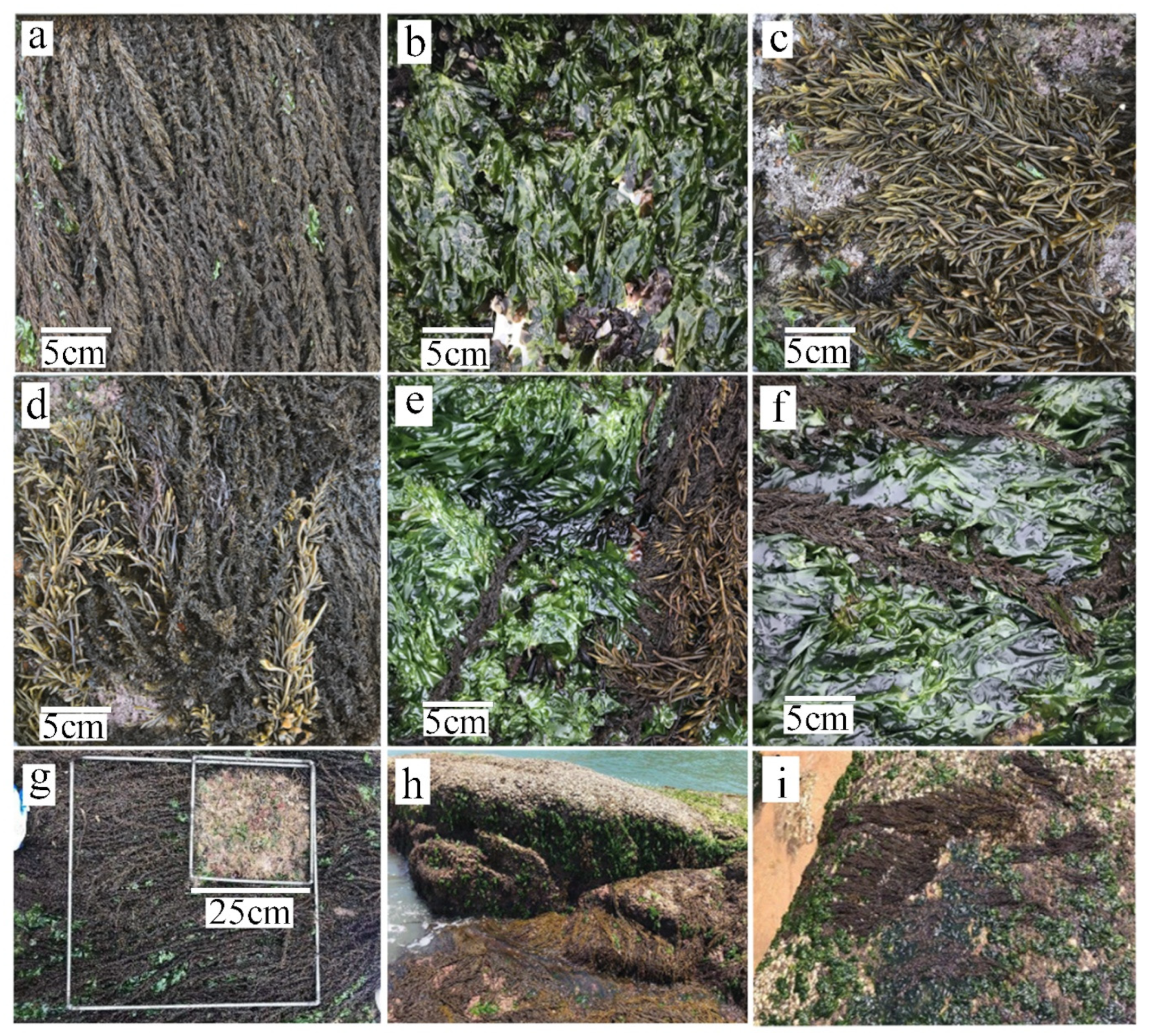
After UAV aerial photography, samples were collected immediately and the biomass values of the target species of seaweed were measured. Ulva pertusa, Sargassum thunbergii and Sargassum fusiforme were the target species used in this investigation (Figure 4).

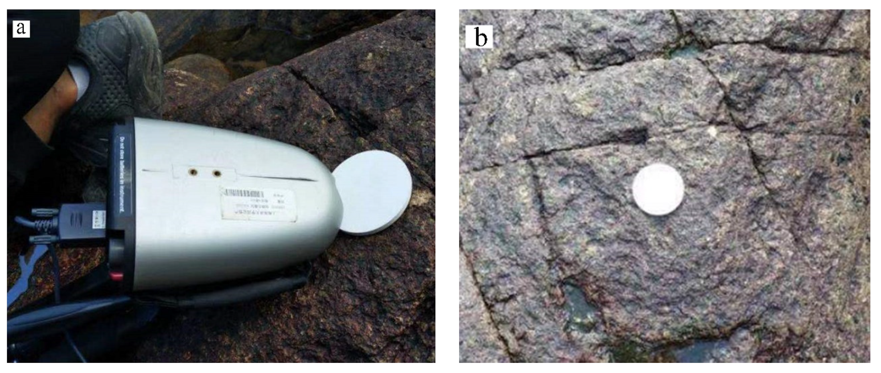
According to the marine survey specifications [36], 0.25 × 0.25 m (length area) quadrats were used for seaweed collection, and the longitude and latitude of the collection points were recorded. Due to the tide, a total of 57 quadrats were collected. In addition, seaweed in different seasons and different dry and wet states in the intertidal zone were measured by an ASD hyperspectral spectrometer (ASD Field Spec Handheld, Analytical Spectral Devices, Inc., Boulder, CO, USA) (Figure 5).

During hyperspectral measurement, it is important to monitor weather factors such as wind speed, humidity, sun direction and elevation. The test was conducted at noon (about 11:00–13:00), and the relevant personnel wore dark clothes. Before spectral measurement, the lens of the instrument needs to be aligned with a white board to correct the dark current and standard white board. When the spectral reflectance curve of the standard whiteboard is a straight line, the spectral measurement can be carried out. Spectrometer optimization was performed every 10–15 min, and dark currents were collected every 5 min [37]. After the hyperspectral determination of the three species of target seaweed, the spectral data were analyzed and the appropriate spectral combination was selected.

2.3. Analysis Method

For seaweed biomass data processing, after the collected seaweeds were placed in a dry area for 6 h, the fresh weight of each of the three seaweed species in every quadrat was measured by an electronic scale, and the biomass, longitude and latitude of Ulva pertusa, Sargassum thunbergii and Sargassum fusiforme collected at each sample point were recorded as a label set. For UAV data processing, before each take-off, we took measurements with the aircraft about 1.5 m above the correction plate to obtain the standard reflectance under the conditions at the time. Taking the orthoimagery of the study area as the reference, 30 reference points were selected at different positions of the image for the geometric fine correction of the multispectral image.

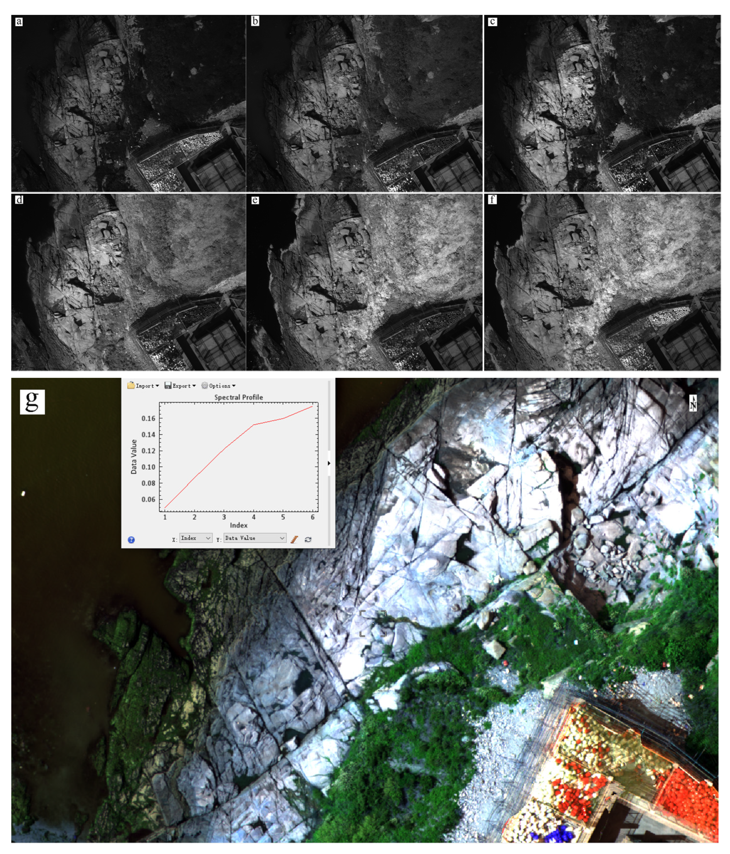
We then preprocessed the raw data (Figure 6) to generate a 6-band image file (Figure 6). Firstly, the registration parameters were generated according to the pixel size, focal length and flight altitude. Then, the generated registration parameters were used as camera parameters for band registration. The calibration gray board was used for radiometric calibration, and the standard reflectivity of the calibration gray board was used as the input (in this paper, bands 1–6 had values of 0.6, 0.62, 0.62, 0.62 and 0.6, respectively). After that, we performed geometric correction according to the ground control points. Finally, the image was spliced to generate an orthophoto image, which was then verified. After verification, the geometric correction error of the image was less than 0.5 pixels.

We selected the region of interest (ROI) according to the coordinates of the ground sampling points. Taking the average reflectance spectrum value of the ground objects within the ROI range as the seaweed reflectance spectrum of the sampling point, the reflectance spectrum data of various points were obtained. According to Equation (1), the spatial resolution (GSD) of the multispectral images in this survey was about 0.058 m, while the quadrat size used for field acquisition was 0.25 × 0.25 m, so a 4-pixel grid on the image was used as the extraction range of image spectral features corresponding to each sample point. In ArcGIS 10.2 (ESRI, Redlands, California, USA), the vector data of the sampling point distribution are established according to the longitude and latitude of the field sampling points. We loaded the sampling point distribution vector data and the spliced UAV remote sensing image data simultaneously into the ENVI5.1 software (Exelis VIS, USA) and established a grid with the sample point as the center, with a size of 4 × 4 and a total of 57 ROI. The average spectral features corresponding to the UAV images in the range of interest of all 57 sample points were extracted as the characteristic parameter set for the seaweed biomass inversion.

$$\frac{a}{GSD}=\frac{f}{h}$$

(1)

h: flight altitude; f: principal distance of lens; GSD: ground resolution; α: pixel size.

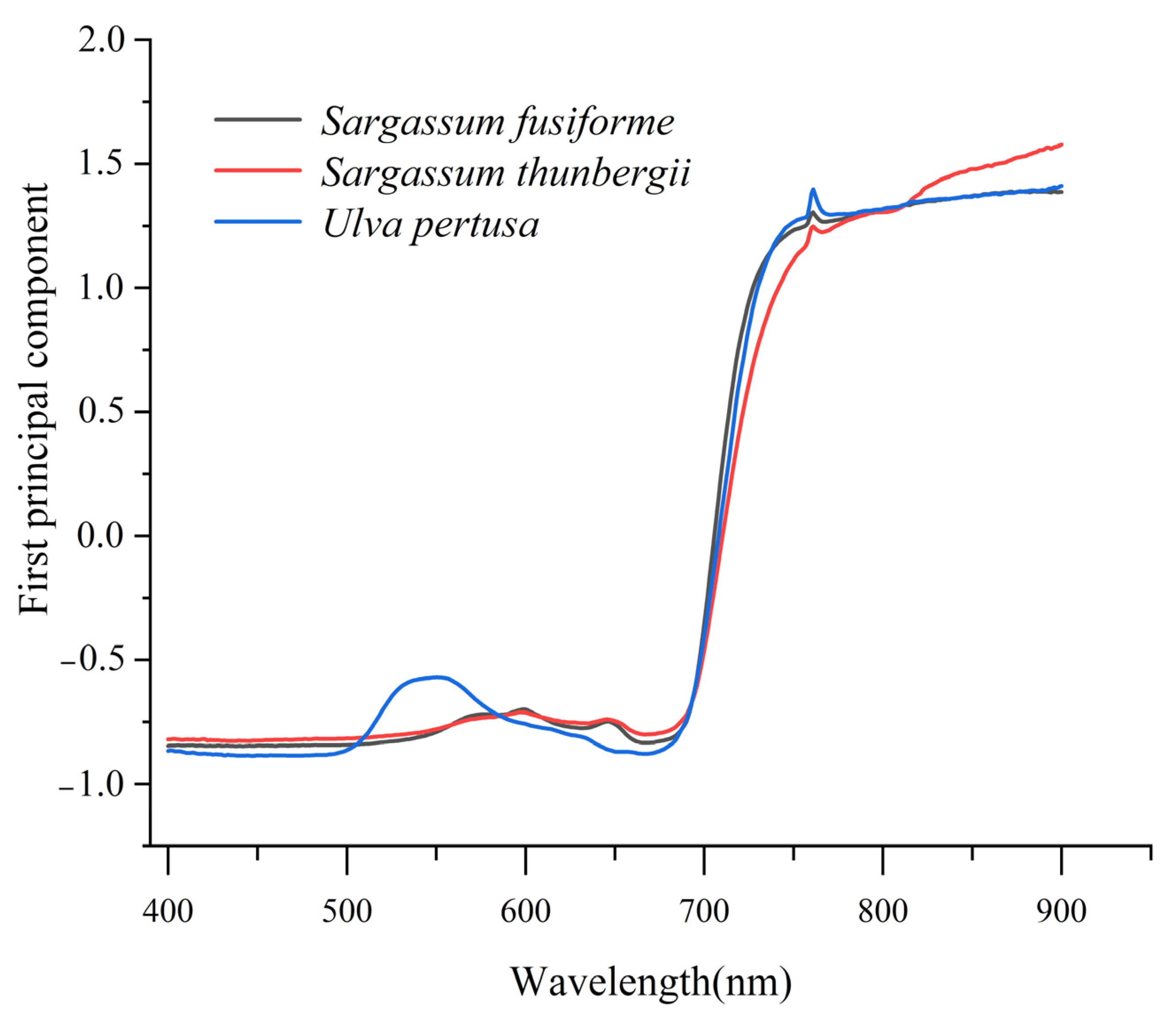
To concisely analyze the spectral data of Ulva pertusa, Sargassum thunbergii and Sargassum fusiforme in different growth states or dry and wet states, principal component analysis (PCA) was used to reduce their dimensions. Information extraction is carried out for multiple variables, and fewer variables are used to replace as much information as possible in the original data, which makes the original problem easier to deal with [38]. After performing the PCA of the spectral data of different states of each seaweed, the load of their principal components was analyzed, and the principal component parameters of high load were used to represent a certain seaweed. According to the research results of Chen [37], the PCA shows that the load of the first principal component of the three seaweeds is greater than 90%, that is, the first principal component can be used to represent more than 90% of the spectral information of a certain seaweed (Figure 7).

Ulva pertusa is similar to terrestrial vegetation. In the visible range, chlorophyll has two strong absorption peaks, a blue band and a red band, centered at 450 nm and 640–680 nm, respectively, and the absorption peak appears at 670 nm. A strong reflection peak appears in the green band of about 550 nm, at which time, the chlorophyll absorption coefficient is the smallest. Near 700 nm, it is also the corresponding valley band of chlorophyll absorption. Therefore, 550 nm and 700 nm accessories are often selected as the characteristic bands of anti-interference to weaken the photosynthetic effective radiation caused by non-photosynthetic substances. The 700–780 nm red-edge range is the climbing ridge of the high-reflection platform formed by the strong absorption of chlorophyll in the red-edge band and multiple scattering in the near-red band. This range is very sensitive to vegetation nutrition, growth and water [39].

As for the method of screening spectral band combinations, Juan et al. selected spectral bands through a genetic programming (GP) framework, which has a better effect in distinguishing and classifying tropical biological communities [40]. In addition, different spectral indices will affect each other [41]. Meanwhile, the 719 nm water vapor absorption band is considered as a potential solar-induced chlorophyll fluorescence (SIF) inversion band [42]. Joiner et al. successfully retrieved SIF spectra from GOME-2 through the 712–747 nm band [43]. Although the seaweeds were exposed to air during UAV aerial photography, their surfaces are still in contact with seawater. Therefore, we tried to optimize the vegetation index with the red-edge band. Further, 20 commonly used vegetation biomass inversion spectral parameters (Table 1) were selected to establish the inversion model and predict the biomass of seaweeds. Combined with the analysis results of the seaweed spectra, 20 spectral parameters were optimized. The specific optimization method is to replace the red band with the red-edge band to adapt to the vegetation index in the seaweed biomass assessment. Taking NDVI as an example, taking the step of a as 0.1 and the value as [0, 1], different vegetation indices are obtained. By observing the correlation coefficient between them and the biomass of each species of seaweed, the maximum value is taken. Through this analysis, it is concluded that the parameters are the best when evaluating seaweed biomass (Table 1).

$$\frac{NIR-\left[aR+\left(1-a\right)Edge\right]}{NIR+\left[aR+\left(1-a\right)Edge\right]},a\in \left[0,1\right]$$

(2)

NIR: near-infrared band; Edge: red-edge band; R: red band; a: optimization coefficient.

Table 1. Calculation formulae of spectral index.

Spectral Index	Pre-Implementation Formula	Improved Formula
NDVI	$\frac{NIR-R}{NIR+R}$	$\frac{NIR-Edge}{NIR+Edge}$
RVI	$\frac{NIR}{R}$	$\frac{NIR}{\left(0.2R+0.8Edge\right)}$
DVI	$NIR-R$	$NIR-\left(0.2R+0.8Edge\right)$
PVI	$\frac{NIR-10.489R-6.604}{\sqrt{\left(1+{10.489}^2\right)}}$	$\frac{NIR-10.489\left(0.6R+0.4Edge\right)-6.604}{\sqrt{\left(1+{10.489}^2\right)}}$
EVI	$2.5\times \frac{NIR-R}{\left(NIR+6R-7.5B+1\right)}$	$2.5\times \frac{NIR-R}{\left(NIR+6R-7.5B+1\right)}$
GNDVI	$\frac{NIR-G}{NIR+G}$	$\frac{NIR-G}{NIR+G}$
RDVI	$\frac{NIR-R}{\sqrt{\left(NIR+R\right)}}$	$\frac{NIR-Edge}{\sqrt{\left(NIR+Edge\right)}}$
SAVI	$\frac{\left(NIR-R\right)\left(1+L\right)}{NIR+R+L}$	$\frac{\left(NIR-Edge\right)\left(1+L\right)}{NIR+Edge+L}$
OSAVI	$\frac{NIR-R}{NIR+R+L}$	$\frac{NIR-Edge}{NIR+Edge+L}$
NLI	$\frac{NI{R}^2-R}{NI{R}^2+R}$	$\frac{NI{R}^2-Edge}{NI{R}^2+Edge}$
GRVI	$\frac{NIR}{G}$	$\frac{NIR}{G}$
GBNDVI	$\frac{NIR-\left(G+B\right)}{NIR+\left(G+B\right)}$	$\frac{NIR-\left(G+B\right)}{NIR+\left(G+B\right)}$
GRNDVI	$\frac{NIR-\left(G+R\right)}{NIR+\left(G+R\right)}$	$\frac{NIR-\left(G+Edge\right)}{NIR+\left(G+Edge\right)}$
BNDVI	$\frac{NIR-B}{NIR+B}$	$\frac{NIR-B}{NIR+B}$
MSAVI	$\frac{2NIR+1-\sqrt{{(2NIR+1)}^2-\left(8NIR-R\right)}}{2}$	$\frac{2NIR+1-\sqrt{{(2NIR+1)}^2-\left(8NIR-Edge\right)}}{2}$
RBNDVI	$\frac{NIR-\left(R+B\right)}{NIR+\left(R+B\right)}$	$\frac{NIR-\left(Edge+B\right)}{NIR+\left(Edge+B\right)}$
Pan NDVI	$\frac{NIR-\left(G+R+B\right)}{NIR+\left(G+R+B\right)}$	$\frac{NIR-\left(G+R+B\right)}{NIR+\left(G+R+B\right)}$
GCI	$\frac{NIR}{G}-1$	$\frac{NIR}{G}-1$
CI red edge	$\frac{NIR}{Red edge}-1$	$\frac{NIR}{Red edge}-1$
VARI	$\frac{G-R}{G+R-B}$	$\frac{G-Edge}{G+Edge-B}$

Table 1. Calculation formulae of spectral index.

Spectral Index	Pre-Implementation Formula	Improved Formula
NDVI	$\frac{NIR-R}{NIR+R}$	$\frac{NIR-Edge}{NIR+Edge}$
RVI	$\frac{NIR}{R}$	$\frac{NIR}{\left(0.2R+0.8Edge\right)}$
DVI	$NIR-R$	$NIR-\left(0.2R+0.8Edge\right)$
PVI	$\frac{NIR-10.489R-6.604}{\sqrt{\left(1+{10.489}^2\right)}}$	$\frac{NIR-10.489\left(0.6R+0.4Edge\right)-6.604}{\sqrt{\left(1+{10.489}^2\right)}}$
EVI	$2.5\times \frac{NIR-R}{\left(NIR+6R-7.5B+1\right)}$	$2.5\times \frac{NIR-R}{\left(NIR+6R-7.5B+1\right)}$
GNDVI	$\frac{NIR-G}{NIR+G}$	$\frac{NIR-G}{NIR+G}$
RDVI	$\frac{NIR-R}{\sqrt{\left(NIR+R\right)}}$	$\frac{NIR-Edge}{\sqrt{\left(NIR+Edge\right)}}$
SAVI	$\frac{\left(NIR-R\right)\left(1+L\right)}{NIR+R+L}$	$\frac{\left(NIR-Edge\right)\left(1+L\right)}{NIR+Edge+L}$
OSAVI	$\frac{NIR-R}{NIR+R+L}$	$\frac{NIR-Edge}{NIR+Edge+L}$
NLI	$\frac{NI{R}^2-R}{NI{R}^2+R}$	$\frac{NI{R}^2-Edge}{NI{R}^2+Edge}$
GRVI	$\frac{NIR}{G}$	$\frac{NIR}{G}$
GBNDVI	$\frac{NIR-\left(G+B\right)}{NIR+\left(G+B\right)}$	$\frac{NIR-\left(G+B\right)}{NIR+\left(G+B\right)}$
GRNDVI	$\frac{NIR-\left(G+R\right)}{NIR+\left(G+R\right)}$	$\frac{NIR-\left(G+Edge\right)}{NIR+\left(G+Edge\right)}$
BNDVI	$\frac{NIR-B}{NIR+B}$	$\frac{NIR-B}{NIR+B}$
MSAVI	$\frac{2NIR+1-\sqrt{{(2NIR+1)}^2-\left(8NIR-R\right)}}{2}$	$\frac{2NIR+1-\sqrt{{(2NIR+1)}^2-\left(8NIR-Edge\right)}}{2}$
RBNDVI	$\frac{NIR-\left(R+B\right)}{NIR+\left(R+B\right)}$	$\frac{NIR-\left(Edge+B\right)}{NIR+\left(Edge+B\right)}$
Pan NDVI	$\frac{NIR-\left(G+R+B\right)}{NIR+\left(G+R+B\right)}$	$\frac{NIR-\left(G+R+B\right)}{NIR+\left(G+R+B\right)}$
GCI	$\frac{NIR}{G}-1$	$\frac{NIR}{G}-1$
CI red edge	$\frac{NIR}{Red edge}-1$	$\frac{NIR}{Red edge}-1$
VARI	$\frac{G-R}{G+R-B}$	$\frac{G-Edge}{G+Edge-B}$

While many new vegetation indices have a good correlation with biomass, if the approximate linear relationship between vegetation indices is ignored, the model may become unstable. Some vegetation indices are significantly hidden from biomass images, and some regression coefficient symbols are inconsistent with the actual significance [44]. Therefore, it is necessary to calculate the variance inflation factor (VIF) of the vegetation index of the input model (Appendix A) to analyze the multicollinearity between variables.

$$V_{IF}=1/\left(1-R^2\right)$$

(3)

V_IF: V_IF between vegetation indices;

R: Correlation coefficient between vegetation indices.

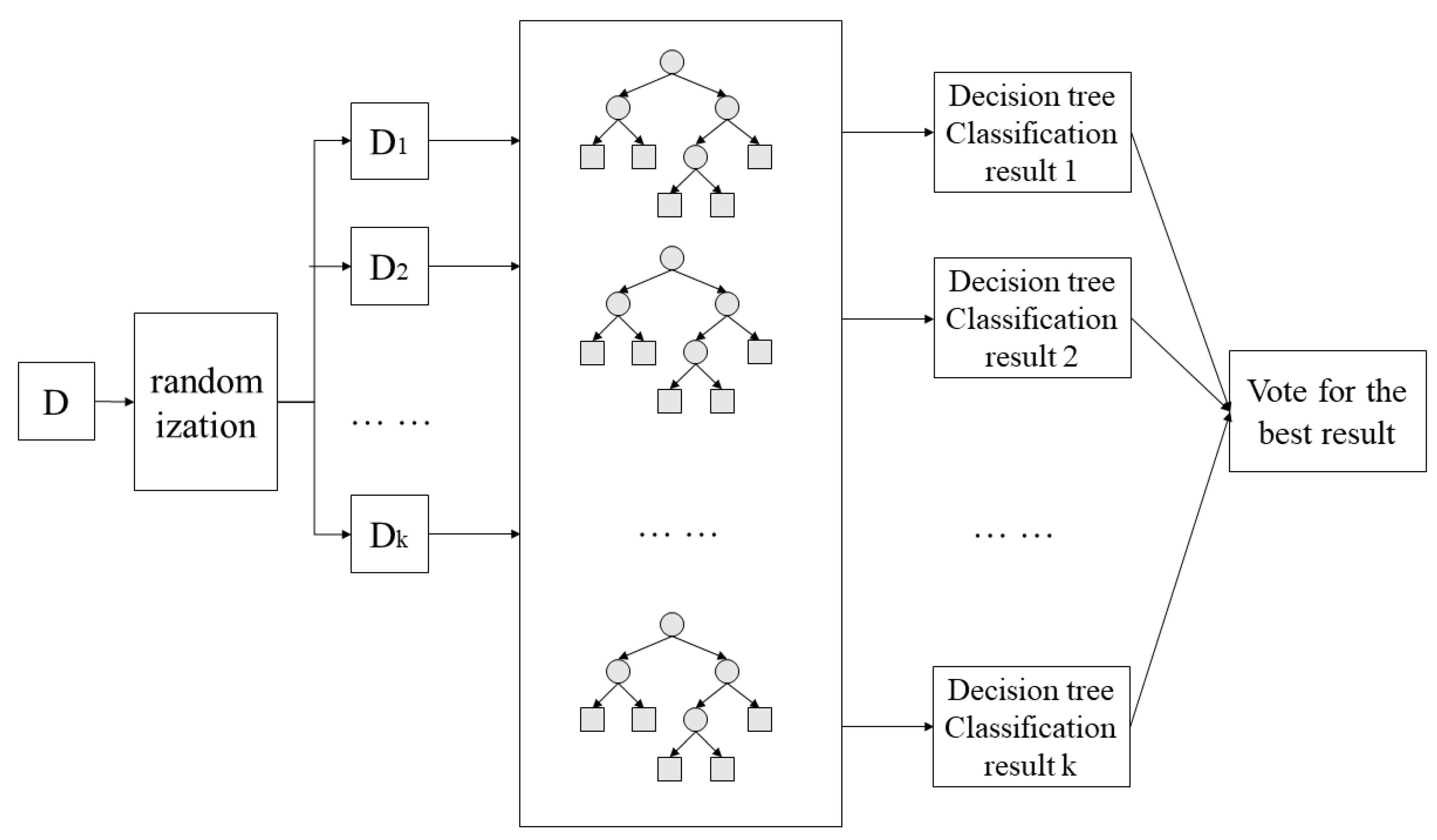
The 20 groups of UAV spectral characteristic data extracted through the ROI range are read and sorted into separate tables with the biomass data of the seaweeds to analyze the relationship between various parameters and biomass, and to carry out inversion evaluation and analysis of the biomass. The data processing and analysis stages were programmed based on PyCharm2020.1 x64 (JetBrains, Prague, Czech Republic). The significance (p value) between the biomass and 20 spectral parameters and three seaweeds was calculated by one-way ANOVA. The correlation coefficient between the biomass and the 20 spectral parameters was calculated by Pearson’s correlation analysis to analyze the response of each seaweed to different spectral parameters. At the same time, in order to compare the advantages of machine learning methods in the quantitative inversion of seaweed in the intertidal zone, two machine learning methods, namely, GBDT (Figure 8) and RF (Figure 9), were used to compare the biomass estimation results.

Additionally, the determination coefficient (R²), root mean square error (RMSE) and mean absolute error (MAE) were selected as the evaluation indices, and the prediction results of the model were evaluated, as shown in Equations (4)–(6). Finally, the results were evaluated in parallel by Lin’s Concordance Correlation Coefficient (LCCC).

$$R^2=\frac{{{\displaystyle \sum }}_{i=1}^n{\left(x_i-\overline{x}\right)}^2{\left(y_i-\overline{y}\right)}^2}{{{\displaystyle \sum }}_{i=1}^n{\left(x_i-\overline{x}\right)}^2{{\displaystyle \sum }}_{i=1}^n{\left(y_i-\overline{y}\right)}^2}$$

(4)

$$RMSE=\sqrt{\frac{{{\displaystyle \sum }}_{i=1}^n{\left(y_i-\widehat{y_i}\right)}^2}{n}}$$

(5)

$$MAE=\frac{{{\displaystyle \sum }}_{i=1}^n\left|y_i-\widehat{y_i}\right|}{n}$$

(6)

3. Result

3.1. Relationship between Biomass and Spectral Parameters

Pearson’ s correlation coefficients between the vegetation index and biomass before and after 20 improvements are listed in

Table 2. Pearson’s correlation coefficients between original vegetation index and biomass.

Spectral Parameters	Ulva pertusa	Sargassum thunbergii	Sargassum fusiforme
NDVI	0.17	0.24 *	0.31 *
RVI	0.14	0.25 *	0.28 *
DVI	0.15	0.27 *	0.35 **
PVI	0.24 *	0.22	0.43 **
EVI	0.20	0.25	0.36 **
GNDVI	0.11	0.35 **	0.14
RDVI	0.17	0.25 *	0.31 *
SAVI	0.17	0.27 *	0.36 **
OSAVI	0.18	0.26 *	0.35 **
NLI	0.19	0.26 *	0.38 **
GRVI	0.38 **	0.48 **	0.03
GBNDVI	0.06	0.35 **	0.20
GRNDVI	0.01	0.32 *	0.21
BNDVI	0.04	0.26	0.35
MSAVI	0.17	0.27 *	0.35 **
RBNDVI	0.09	0.27 *	0.25
Pan NDVI	0.01	0.33 **	0.22
GCI	0.38 **	0.48 **	0.03
CI red edge	0.15	0.40 **	0.20
VARI	0.74 **	0.38 **	0.39 **

* means p < 0.05, ** means p < 0.01.

and

Table 3. Pearson’s correlation coefficients between improved vegetation index and biomass.

Spectral Parameters	Ulva pertusa	Sargassum thunbergii	Sargassum fusiforme
NDVI	0.34 *	0.39 **	0.31 *
RVI	0.33 *	0.37 **	0.40 **
DVI	0.34 *	0.27	0.35 **
PVI	0.18	0.38 **	0.43 **
EVI	0.34 *	0.30 *	0.36 **
GNDVI	0.11	0.35 **	0.30
RDVI	0.34 *	0.39 **	0.31 *
SAVI	0.35 **	0.27	0.36 **
OSAVI	0.35 **	0.34 *	0.27
NLI	0.24	0.40 **	0.31 *
GRVI	0.38 **	0.48 **	0.49 **
GBNDVI	0.06	0.35 **	0.38 **
GRNDVI	0.14	0.32 *	0.32 *
BNDVI	0.04	0.26 *	0.21
MSAVI	0.34 *	0.27 *	0.29
RBNDVI	0.23	0.34 *	0.21
Pan NDVI	0.01	0.33 *	0.35 **
GCI	0.38 **	0.48 **	0.49 **
CI red edge	0.15	0.40 **	0.25
VARI	0.77 **	0.39 **	0.39 **

* means p < 0.05, ** means p < 0.01.

.

When the correlation is significant (Table 2), the absolute value of the correlation coefficient (Figure 4) is greater, indicating that there is no special case where the correlation coefficient is large but not significant due to the number of samples not meeting the requirements. There were few significant values between the biomass of Ulva pertusa and the 20 spectral parameters. Apart from being significantly (p < 0.05) or very significantly (p < 0.01) related to PVI, GRVI, CVI and VARI, it was not significantly related to any other spectral parameters. Its Pearson’s correlation coefficients were generally lower than the other three seaweeds, but VARI showed a significant and strong correlation. Except for PVI, EVI and BNDVI, the biomass of Sargassum thunbergii showed significant or extremely significant correlations with the spectral parameters, and the Pearson’s correlation coefficients showed a medium correlation. The biomass of Sargassum fusiforme showed significant correlation with NDVI, RVI and RDVI, and an extremely significant correlation with DVI, PVI, EVI, SAVI, OSAVI, NLI, MSAVI and VARI. Through comparative analysis of Table 2 and Table 3, the correlation coefficient is improved overall, with a maximum increase of 0.17. The results of one-way ANOVA between the partial recalculated vegetation index and biomass were significant (p < 0.05).

The VIF was calculated according to the 20 spectral indices with the highest correlation with biomass. The results of a multicollinearity analysis between two vegetation indices are shown in Appendix A. According to the analysis in the Appendix A, there was essentially no collinearity between the 20 variables. These analysis results can help to avoid the over-fitting phenomenon of the model.

3.2. Model Analysis

We consulted the GradientBoostingRegressor and RandomForestRegressor in the scikit-learn library to establish the GBDT and RF biomass regression models. We divided the sorted data into a training set and test set according to a 3:1 ratio. The evaluation index uses R², RMSE and MAE to calculate the training and test sets, respectively. In GBDT, n_estimators and learning rates must be considered, where n_estimators is the maximum number of iterations of weak learners (the maximum number of weak learners). If it is too small, it will easily lead to under-fitting of the model; otherwise, if it is too large, it will lead to over-fitting. The learning rate is the weight reduction coefficient of each weak learner, that is, the shrinkage step used in the update process.

Using the parameter search method (Grid Search) in the two-dimensional parameter matrix (in n_estimators and learning rate), all points in the grid are traversed in turn to be input as the model parameter. The R² and other evaluation parameters of the corresponding training set are obtained by the K-CV method. Finally, the best n_estimators and learning rate in the training set are used as the best parameters to calculate the test set. The global optimization can be obtained by using the Grid Search, and n_estimators and learning rates are made independent of each other for parallel optimization. In this paper, CV is set to 4, n_estimators range from 100 to 1000 in steps of 10, and the learning rate ranges from 0 to 1 in steps of 0.1. The best GBDT model of Ulva pertusa had n_estimators and a learning rate of 110 and 0.6, respectively. The best GBDT model of Sargassum thunbergii and Sargassum fusiforme had n_estimators and a learning rate of 100 and 0.5, respectively.

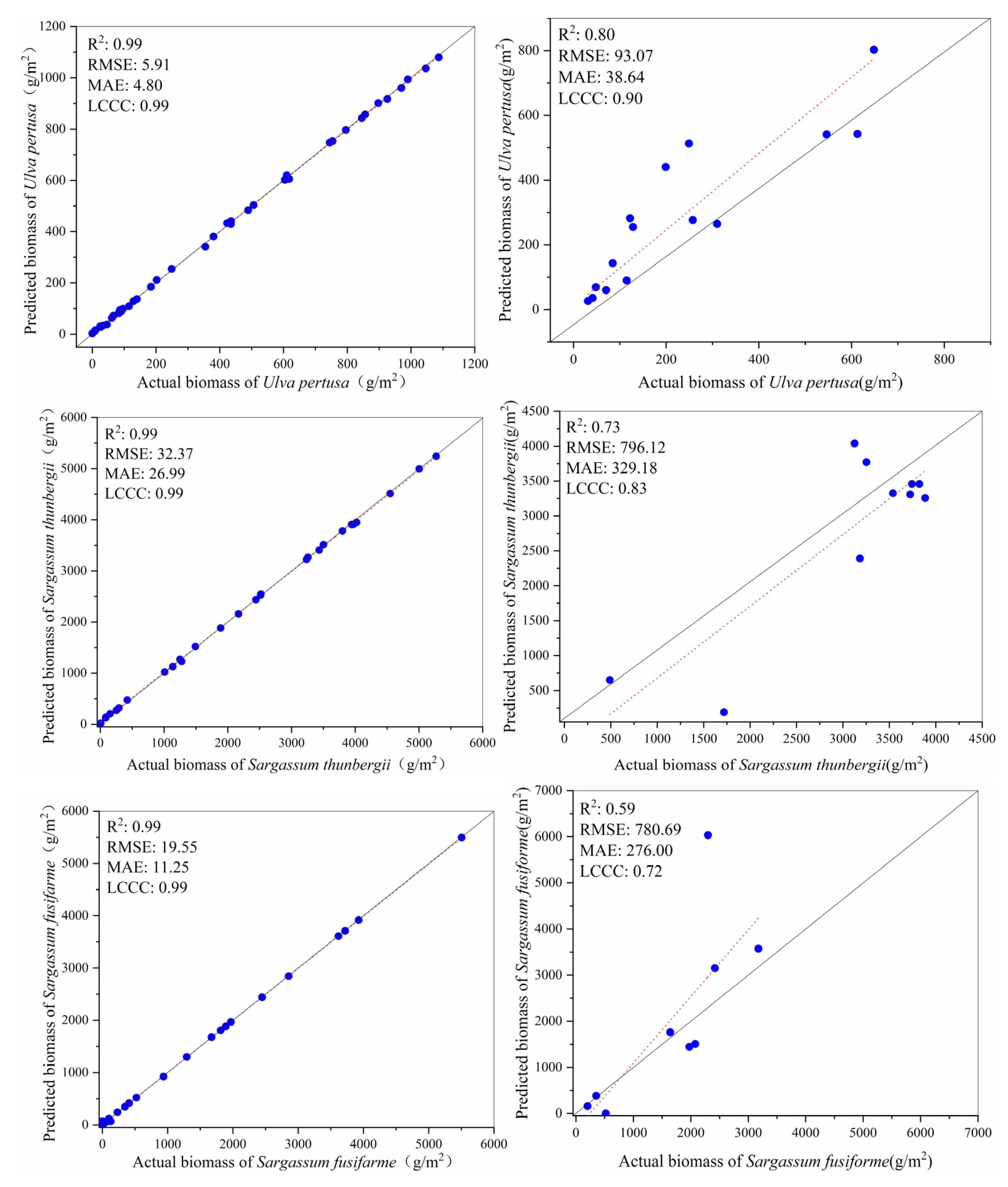
In the in situ quadrat survey, Ulva pertusa could be collected in each quadrat, but there were few Sargassum thunbergii and Sargassum fusiforme, and in some quadrats they were not collected. Therefore, in quadrats without Sargassum thunbergii and Sargassum fusiforme, the biomass of these two seaweeds was 0, so they were removed before model calculation. Numpy and R2_Score in PyCharm calculate R², RMSE and MAE of the training and test sets and outputs them (Figure 10). Similarly, the random forest model is used to obtain their evaluation indices.

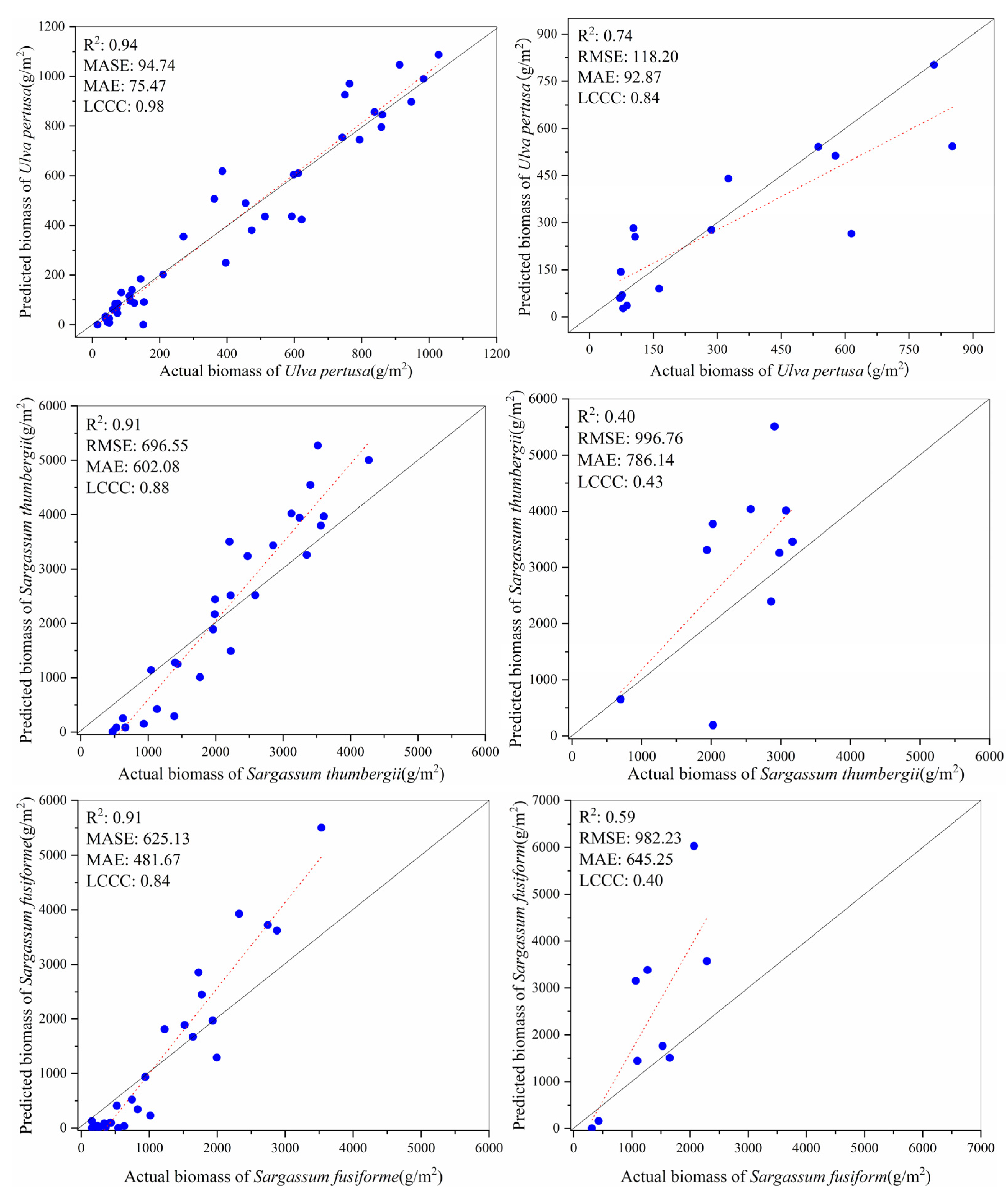
The RF model’s parameters are mainly n_estimators and max depth, which are also optimized by Grid Search. n_estimators represents the number of sub-datasets generated by replacement sampling of the original dataset, that is, the number of decision trees. If it is too small, it is easy to under-fit, while being too large will lead to over-fitting. Max depth represents the maximum depth of the decision tree and limits the depth of the subtree when the decision tree constructs the optimal model. These two parameters are optimized by the Grid Search method, and n_estimators ranges from 10 to 200 in steps of 1 and max depth ranges from 1 to 20 in steps of 1. According to the optimal parameters, the evaluation indices of different seaweed are obtained (Figure 11).

Comparing the three evaluation indices, among the two machine learning methods, the accuracy of the prediction indices of GBDT is the highest, which is 0.06, 0.33 higher than that of RF; RMSE decreased by 25.13 g/m², 200.64 g/m² and 201.54 g/m² and MAE decreased by 54.80 g/m², 456.96 g/m², 369.25 g/m². Thus, GBDT is superior to the RF inversion method when analyzing the biomass regression of seaweed in an intertidal zone.

3.3. Model Application

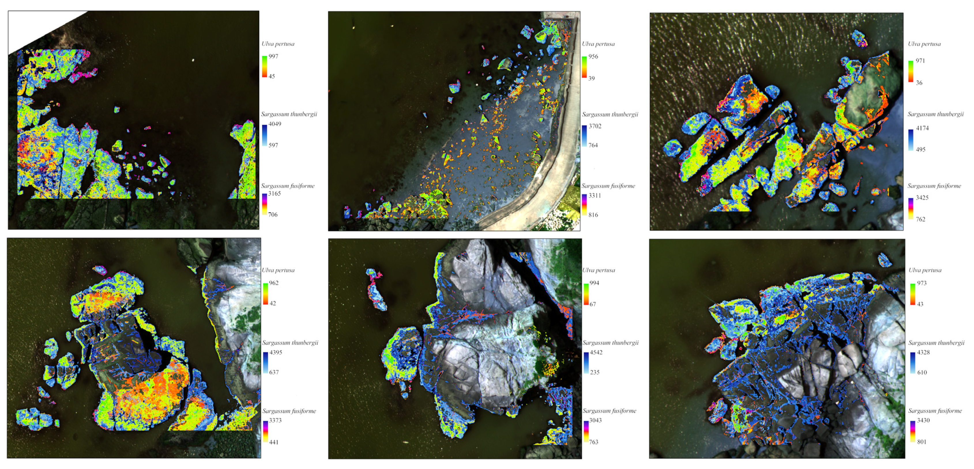
Through the above three machine learning models combined with the sampled biomass data, the biomass values of three species of intertidal seaweed were evaluated. It is concluded that the effect is best when the GBDT model is used for the quantitative inversion of biomass. Using Python’s GDAL Library (3.4.2) and the GBDT model, the quantitative inversion of the seaweed species was carried out on the UAV aerial photography data, and three representative quantitative inversion maps of the study area were obtained (Figure 12).

The biomass values of Ulva pertusa, Sargassum thunbergii and Sargassum fusiforme in the sample area were 36–971 g/m² (R² = 0.80, RMSE = 93.1 g/m²), 495–4174 g/m² (R² = 0.73, RMSE = 790.1 g/m²) and 762–3425 g/m² (R² = 0.59, RMSE = 780.7 g/m²), respectively. Ulva pertusa has the widest distribution range, and its biomass increases gradually along the offshore direction. However, in the area close to the sea surface, Sargassum thunbergii and Sargassum fusiforme are distributed most often. Because the plant height of Ulva pertusa is lower than Sargassum fusiforme and Sargassum thunbergii, Ulva pertusa is shielded by the two other seaweeds in the area close to the sea surface. Since the UAV shooting time was during the lowest of the spring tides, it can be seen from the figure that Sargassum thunbergii grows mainly in the middle tide area. Sargassum fusiforme is often distributed in the subtidal zone, so there are not many Sargassum fusiforme individuals in the figure, and the actual sample size is also small (in the same quadrat, Ulva pertusa and Sargassum thunbergii are more abundant).

The seaweed biomass values in the study area are Ulva pertusa: the average value is 692.74 g/m², and the standard deviation is 163.52 g/m²; Sargassum fusiforme: the average value is 1897.13 g/m², and the standard deviation is 404.58 g/m²; Sargassum thunbergii: the average value is 2027.95 g/m², and the standard deviation is 590.93 g/m², which are consistent with the statistical results. Based on the inherent natural grouping in the data, the natural discontinuity classification (Jenks) is used to group them. The grouping is set at the position with large difference in data values, the seaweed biomass in the sample area is divided into five levels, and the proportions of pixels in each level are counted (

Table 4. Biomass classification of Ulva pertusa in the sample area based on GBDT model inversion.

Biomass Grade	Biomass (g/m2)	Proportion/%
I	36–377	4.3
II	377–583	19.5
III	583–705	27.0
IV	705–816	19.5
V	816–971	29.7

,

Table 5. Biomass classification of Sargassum fusiforme in the sample area based on GBDT model inversion.

Biomass Grade	Biomass (g/m2)	Proportion/%
I	762–1484	21.7
II	1484–1862	10.6
III	1862–2105	35.7
IV	2105–2394	25.6
V	2394–3425	6.4

and

Table 6. Biomass classification of Sargassum thunbergii in the sample area based on GBDT model inversion.

Biomass Grade	Biomass (g/m2)	Proportion/%
I	495–1320	13.6
II	1320–1803	19.1
III	1803–2228	30.6
IV	2228–2760	26.2
V	2760–4174	10.5

).

The identification results show that Sargassum thunbergii and Sargassum fusiforme biomass in the sample area is mainly belonging to grade III and grade IV, and Ulva pertusa is mainly belonging to grade III and grade V. The areas with high biomass grade are distributed in the low-tide zone and middle-tide zone. The high-tidal zone is mainly grade I. The seaweed biomass in the sample area (high-tidal area, middle-tidal area and low-tidal area) is reflected. The change in Ulva pertusa, Sargassum thunbergii and Sargassum fusiforme biomass along the offshore direction is mainly because the closer to the sea surface, the greater the biomass.

4. Discussion

The GBDT model was applied to some representative areas in the UAV images to obtain the distribution characteristics of three typical seaweeds at Gouqi Island (Figure 12): Ulva pertusa is located in the high-, middle- and low-tide zones, and the closer it is to the low-tide zone, the greater its biomass [45]. Sargassum thunbergii is mainly distributed in the mid-tidal zone and low-tidal zone, and Sargassum fusiforme is mainly distributed in the low-tidal zone [46]. The main source of error in seaweed biomass inversion is the mutual masking between seaweeds. When the biomass is large, because most of the biomass is covered by other seaweeds, the inversion accuracy decreases significantly. R² of Ulva pertusa is 0.8, RMSE is 93.07 g/m², and MAE is 39.6493.07 g/m²; R² of Sargassum thunbergii is 0.73, RMSE is 796.1293.07 g/m², and MAE is 329.1893.07 g/m²; R² of Sargassum fusiforme is 0.59, RMSE is 780.6993.07 g/m², and MAE is 276.0093.07 g/m².

Using the slope data recorded at each sampling point, seaweeds were found to be distributed in the nearshore area within the range of 0–90°. Through statistical analysis, we found that the growth distribution of the three seaweeds had no correlation with the slope. However, the slope will affect the inversion results. Because the direction of UAV aerial photography is vertical to the ground, when the slope is near vertical, the predicted value will be underestimated. Quadrat data with too large a slope were eliminated (>25°), and the accuracy was improved by 0.14.

According to Figure 10 and Figure 11, the predicted value deviates from the 45° line of y = X. Being below the line indicates that the predicted value is smaller than the actual value, while being above the line indicates that the predicted value is larger than the actual value. In terms of this situation in combination with the actual site situation (Figure 12), firstly, the predicted value is too small. This could be caused by the slope. Subsequent research may need to introduce DEM data for point cloud computing to make the calculation results more accurate.

In addition, different sediment types, small red seaweeds, mussels and other attachments on the bedrock, epiphytic seaweeds, etc., will have a certain impact on the spectral values in the quadrat. The bedrock types of seaweed growth mainly include rocks and bedrock with mussels and red seaweeds attached, which almost have a relatively fixed form. Furthermore, due to the scouring of seawater, Sargassum fusiforme and Sargassum thunbergii are mostly distributed in parallel strips near the shore. Therefore, subsequent research could improve the spatial resolution of the data so as to introduce the Gray Level Co-occurrence Matrix to calculate the texture parameters as the input parameters, improving the evaluation accuracy [47].

5. Conclusions

At present, there are few studies on the application of remote sensing to the biomass assessment of seaweed. In this study, we used GBDT and RF algorithms, combined with hyperspectral data to improve the spectral index. We quantitatively retrieved the multispectral UAV image data on intertidal seaweed beds, and obtained the biomass and distribution values of three species of seaweed: Ulva pertusa, Sargassum thunbergii and Sargassum fusiforme (R² = 0.8, 0.73 and 0.59, respectively). This method can also be applied to assess the biomass of other seaweed beds and other seaweed species.

In the biomass assessment of benthic seaweed in intertidal zones, the red-edge band can improve the estimation accuracy of biomass inversion to a certain extent. By introducing the red-edge band to the traditional vegetation index calculation, the correlation coefficient between the vegetation index and seaweed biomass is increased by 0.02–0.17. The parameter with the best correlation with Ulva pertusa is VARI, Sargassum thunbergii is GCI, and Sargassum fusiforme is best correlated with GCI and NLI, which are the indices optimized by using red edge. We calculate the expansion coefficient between the spectral indices with the highest correlation to exclude multicollinearity between vegetation indices.

The method in this study can be used to improve the evaluation of biomass and blue carbon reserves of nearshore ecosystems, and provides a reference for the investigation of other types of seaweed beds in the intertidal zone. Furthermore, this study provides a theoretical basis and technical support for the quantitative inversion of seaweed biomass in intertidal zones.

References

1. Yamamoto, M.; Fukushima, M.; Liu, D. The effect of humic substances on iron elution in the method of restoration of seaweed beds using steelmaking slag. ISIJ Int. 2012, 52, 1909–1913. [Google Scholar] [CrossRef] [Green Version]
2. Fiblee, D.K.; Feehan, C. Large-scale degradation of a kelp ecosystem in an ocean warming hotspot. Mar. Ecol. Prog. Ser. 2016, 543, 141–152. [Google Scholar]
3. Raven, J. Blue carbon: Past, present and future, with emphasis on macroalgae. Biol. Lett. 2018, 14, 20180336. [Google Scholar] [CrossRef] [PubMed] [Green Version]
4. Schepers, M.; Martens, N.; Tiane, A.; Vanbrabant, K.; Liu, H.B.; Lütjohann, D.; Mulder, M.; Vanmierlo, T. Corrigendum: Edible seaweed-derived constituents: An undisclosed source of neuroprotective compounds. Neural Regen. Res. 2021, 16, 790–795. [Google Scholar]
5. Guastaferro, M.; Reverchon, E.; Baldino, L. Agarose, Alginate and Chitosan Nanostructured Aerogels for Pharmaceutical Applications: A Short Review. Front. Bioeng. Biotechnol. 2021, 9, 688477. [Google Scholar] [CrossRef]
6. Pasae, R.; Maming; Soekendarsi, E. Making of KCl liquid fertilizer from liquid waste manufacture of seaweed and galvanized industry. IOP Conf. Ser. Earth Environ. Sci. 2020, 473, 12076. [Google Scholar] [CrossRef]
7. Wernberg, T.; Filbee-Dexter, K. Missing the marine forest for the trees. Mar. Ecol. Prog. Ser. 2019, 612, 209–215. [Google Scholar] [CrossRef] [Green Version]
8. Niklas, K. Modelling Below- and Above-ground Biomass for Non-woody and Woody Plants. Ann. Bot. 2005, 95, 315–321. [Google Scholar] [CrossRef] [Green Version]
9. Zhang, C.; Zhou, W.; Sun, S.; Song, Z. Seasonal succession of macroalgae community in Naozhou Island. J. Trop. Oceanogr. 2020, 39, 74–84. [Google Scholar]
10. Abualtayef, M.; Rabou, M.A.; Afifi, S.; Rabou, A.F.A.; Seif, A.K.; Masria, A. Change detection of Gaza coastal zone using GIS and remote sensing techniques. J. Coast. Conserv. 2021, 25, 36. [Google Scholar] [CrossRef]
11. Sarhadi, A.; Burn, D.; Johnson, F.; Mehrotra, R.; Sharma, A. Water resources climate change projections using supervised nonlinear and multivariate soft computing techniques. J Hydrol. 2016, 536, 119–132. [Google Scholar] [CrossRef] [Green Version]
12. Pham, Q.; Mohammadpour, R.; Linh, N.; Mohajane, M.; Pourjasem, A.; Sammen, S.; Anh, D.; Nam, V. Application of soft computing to predict water quality in wetland. Environ. Pollut. 2021, 28, 185–200. [Google Scholar] [CrossRef]
13. Lama, G.; Sadeghifar, T.; Azad, M.; Sihag, P.; Kisi, O. On the Indirect Estimation of Wind Wave Heights over the Southern Coasts of Caspian Sea: A Comparative Analysis. Water 2022, 4, 843. [Google Scholar] [CrossRef]
14. Lama, G.F.C.; Crimaldi, M.; Pasquino, V.; Padulano, R.; Chirico, G.B. Bulk Drag Predictions of Riparian Arundo donax Stands through UAV-acquired Multispectral Images. Water 2021, 13, 1333. [Google Scholar] [CrossRef]
15. Fukano, Y.; Guo, W.; Aoki, N.; Ootsuka, S.; Noshita, K.; Uchida, K.; Kato, Y.; Sasaki, K.; Kamikawa, S.; Kubota, H. GIS-Based Analysis for UAV-Supported Field Experiments Reveals Soybean Traits Associated with Rotational Benefit. Front. Plant Sci. 2021, 12, 1003. [Google Scholar] [CrossRef]
16. Zheng, Y.; Wu, J.; Wang, A.; Chen, J. Object- and pixel-based classifications of macroalgae farming area with high spatial resolution imagery. Geocarto Int. 2018, 33, 1–25. [Google Scholar] [CrossRef]
17. Bell, T.; Cavanaugh, K.; Siegel, D. Remote monitoring of giant kelp biomass and physiological condition: An evaluation of the potential for the Hyperspectral Infrared Imager (HyspIRI) mission. Remote Sens. Environ. 2015, 167, 218–228. [Google Scholar] [CrossRef]
18. Cavanaugh, K.C.; Siegel, D.A.; Kinlan, B.P. Scaling giant kelp field measurements to regional scales using satellite observations. Mar. Ecol. Prog. Ser. 2010, 403, 13–27. [Google Scholar] [CrossRef] [Green Version]
19. Ishiguro, E.; Yoshimoto, S.I.; Ishikawa, D. Monitoring of the Environment around Kagoshima Bay Using Remote Sensing Data-Development of Identifying Method for Seaweeds Growing Region. J. Agric. Meteorol. 2005, 60, 409–414. [Google Scholar] [CrossRef] [Green Version]
20. Blakeway, D.; Byers, M.; Stoddart, J.; Rossendell, J. Coral colonisation of an artificial reef in a turbid nearshore environment, Dampier Harbour, western Australia. PLoS ONE 2013, 8, e75281. [Google Scholar] [CrossRef] [Green Version]
21. Rosa, M.; Isabel, S.P.; Sara, C.A.; Isabel, C.; Debora, Borges. Temporal and spatial variation of seaweed biomass and assemblages in Northwest Portugal. J Sea Res. 2021, 174, 102079. [Google Scholar]
22. Thomas, Ē.M. Bell Quantifying Intertidal Macroalgae Abundance Using Aerial Photography on the Isle of Wight. Master’s Thesis, Imperial College London, London, UK, 2015. [Google Scholar]
23. Sindde-Gonzalez, I. Biomass estimation of pasture plots with multitemporal UAV-based photogrammetric surveys. Int. J. Appl. Earth Obs. Geoinf. 2021, 101, 102355. [Google Scholar] [CrossRef]
24. Liu, Y.; Liu, S.; Li, J. Estimating biomass of winter oilseed rape using vegetation indices and texture metrics derived from UAV multispectral images. Comput. Electron. Agr. 2019, 166, 105026. [Google Scholar] [CrossRef]
25. David, A.J.S.; Steven, E.; Hernán, C.; Benítez-Restrepo, D. Novel Feature-Extraction Methods for the Estimation of Above-Ground Biomass in Rice Crops. Sensors 2021, 21, 4369. [Google Scholar]
26. RAO, H.; Shi, X.; Rodrigue, A.K. Feature selection based on artificial bee colony and gradient boosting decision tree. Appl. Soft Comput. 2018, 74, 634–642. [Google Scholar] [CrossRef]
27. Cheng, J.; Li, G.; Chen, X. Research on Travel Time Prediction Model of Freeway based on Gradient Boosting Decision Tree. IEEE Access 2018, 1, 7466–7480. [Google Scholar] [CrossRef]
28. Wujun, D.; Huiying, J.; Yuhong, Z. Detecting temporal changes in the temperature sensitivity of spring phenology with global warming: Application of machine learning in phenological model. Agric. For. Meteorol. 2019, 279, 107702. [Google Scholar]
29. Arabameri, A.; Blaschke, T.; Pradhan, B.; Pourghasemi, H.R.; Tiefenbacher, J.P.; Bui, D.T. Evaluation of Recent Advanced Soft Computing Techniques for Gully Erosion Susceptibility Mapping: A Comparative Study. Sensors 2020, 20, 335. [Google Scholar] [CrossRef] [PubMed] [Green Version]
30. Liu, Y.; Huang, Y.; Sun, Q.; Feng, H.; Yang, G.; Yang, F. Estimation of plant height and above ground biomass of potato based on UAV digital image. Natl. Remote Sens. Bull. 2021, 25, 2004–2014. [Google Scholar]
31. Jiang, F.; Kutia, M.; Ma, K.; Chen, S.; Long, J.; Sun, H. Estimating the aboveground biomass of coniferous forest in Northeast China using spectral variables, land surface temperature and soil moisture. Sci. Total Environ. 2021, 785, 147335. [Google Scholar] [CrossRef] [PubMed]
32. Yang, H.; Li, F.; Wang, W.; Yu, K. Estimating Above-Ground Biomass of Potato Using Random Forest and Optimized Hyperspectral Indices. Remote Sens. 2021, 13, 2339. [Google Scholar] [CrossRef]
33. Clevers, J.G.P.W.; van der Heijden, G.W.A.M.; Verzakov, S.; Schaepman, M.E. Estimating Grassland Biomass Using SVM Band Shaving of Hyperspectral Data. Photogramm. Eng. Rem. S 2007, 73, 1141. [Google Scholar] [CrossRef] [Green Version]
34. Fan, J.; Huang, G.; Chi, M.; Shi, Y.; Jiang, J.; Feng, C.; Yan, Z.; Xu, Z. Prediction of chemical reproductive toxicity to aquatic species using a machine learning model: An application in an ecological risk assessment of the Yangtze River, China. Sci. Total Environ. 2021, 796, 148901. [Google Scholar] [CrossRef]
35. Wu, Z.; Zhang, S. Effect of Typhoon on the Distribution of Macroalgae in the Seaweed Beds of Gouqi Island, Zhejiang Province. J. Agric. Sci. Technol. 2019, 21, 159–168. [Google Scholar]
36. Johnson, M. Estimating intertidal seaweed biomass at larger scales from quadrat surveys. Mar. Environ. Res. 2020, 156, 104906. [Google Scholar] [CrossRef]
37. Chen, J.; Li, X.; Wang, K.; Zhang, S.; Li, J.; Sun, M. Assessment of intertidal seaweed biomass based on RGB imagery. PLoS ONE 2022, 17, 0263416. [Google Scholar] [CrossRef]
38. Li, C.; Dai, Y.; Zhao, J.; Yin, J.X. Remote Sensing Monitoring of Volcanic Ash Clouds Based on PCA Method. Acta Geophys. 2015, 63, 432–450. [Google Scholar] [CrossRef] [Green Version]
39. Gutman, G.; Skakun, S.; Gitelson, A. Revisiting the use of red and near-infrared reflectances in vegetation studies and numerical climate models. Sci. Remote Sens. 2021, 4, 100025. [Google Scholar] [CrossRef]
40. Albarracín, J.; Oliveira, R.; Hirota, M.; dos Santos, J.; Torres, R. A Soft Computing Approach for Selecting and Combining Spectral Bands. Remote Sens. 2020, 12, 2267. [Google Scholar] [CrossRef]
41. Fu, Y.; Yang, G.; Wang, J.; Feng, H. A comparative analysis of spectral vegetation indices to estimate crop leaf area index. Intell. Autom. Soft 2013, 19, 315–326. [Google Scholar] [CrossRef]
42. Guanter, L.; Zhang, Y.; Jung, M. Global and Time-Resolved Monitoring of Crop Photosynthesis with Chlorophyll Fluorescence. Proc. Natl. Acad. Sci. USA 2014, 111, 1327–1333. [Google Scholar] [CrossRef] [Green Version]
43. Joiner, J.; Yoshida, Y.; Guanter, L. New Methods for Retrieval of Chlorophyll Red Fluorescence from Hyper-Spectral Satellite Instruments: Simulations and Application to GOME-2 and SCIAMCHY. Agu Fall Meeting. Copericus Publ. 2016, 9, 3939–3967. [Google Scholar]
44. Xiao, W.; Chen, J.; Xuan, H.; Ren, H.; Zhang, J.; Zhang, L. Inversion and Analysis of Maize Biomass in Coal Mining Subsidence Area Based on UAV Images. Trans. Chin. Soc. Agric. Mach. 2018, 49, 1000–1298. [Google Scholar]
45. Gouraguine, A.; Moore, P.; Burrows, M.; Velasco, E.; Ariz, L.; Luis, F.; Rodrigo, M.; Ltalo, F.; Smale, D.; Alejandro, P. The intensity of kelp harvesting shapes the population structure of the foundation species Lessonia trabeculata along the Chilean coastline. Mar. Biol. 2021, 168, 66. [Google Scholar] [CrossRef]
46. Zollmann, M.; Rubinsky, B.; Liberzon, A.; Golberg, A. Multi-scale modeling of intensive macroalgae cultivation and marine nitrogen sequestration. Commun. Biol. 2021, 4, 848. [Google Scholar] [CrossRef] [PubMed]
47. Jin, W.; Yan, G.; Xiao, W.; Lei, F. Forest Classification Based on Forest texture in Northwest Yunnan Province. IOP Conf. Ser. Earth 2014, 17, 012071. [Google Scholar]
Figure 1. Methodological scheme. The figures in () are the corresponding chapters in this paper.
Remotesensing 14 02143 g001
Figure 2. Study area. (a) is the approximate location of the study area, (b) is the location of aerial photography area in specific research area, (c) is the distribution of sampling stations.
Remotesensing 14 02143 g002
Figure 3. UAV with camera and calibration gray board. (a) is UAV with camera, (b) is calibration gray board.
Remotesensing 14 02143 g003
Figure 4. Seaweed photos. (ac) are Sargassum thunbergii, Ulva pertusa, and Hizikia fusifarme, respectively; (af) are photographs used for analysis (clipping of quadrat), (g) is after sampling, (h,i) are field photographs.
Remotesensing 14 02143 g004
Figure 5. ASD spectrometer and calibration whiteboard. (a) is ASD spectrometer, (b) is calibration whiteboard.
Remotesensing 14 02143 g005
Figure 6. Raw data (6 bands) and preprocessed image (RGB display). (af) are the imaging results six bands of MS600Pro multispectral camera (bands 1–6 respectively), (g) is preprocessing result image displayed through RGB channels.
Remotesensing 14 02143 g006
Figure 7. Spectral reflectance of the first principal component.
Remotesensing 14 02143 g007
Figure 8. The schematic diagram of GBDT.
Remotesensing 14 02143 g008
Figure 9. The schematic diagram of RF.
Remotesensing 14 02143 g009
Figure 10. Prediction indices calculated by GBDT.
Remotesensing 14 02143 g010
Figure 11. Prediction indices calculated by RF.
Remotesensing 14 02143 g011
Figure 12. Biomass inversion map of three kinds of seaweed in three regions based on GBDT.
Remotesensing 14 02143 g012