Abstract
The accurate estimation of spatially explicit forest aboveground biomass (AGB) provides an essential basis for sustainable forest management and carbon sequestration accounting, especially in Myanmar, where there is a lack of data for forest conservation due to operational limitations. This study mapped the forest AGB using Sentinel-2 (S-2) images and Shuttle Radar Topographic Mission (SRTM) based on random forest (RF), stochastic gradient boosting (SGB) and Kriging algorithms in two forest reserves (Namhton and Yinmar) in Myanmar, and compared their performance against AGB measured by the traditional methods. Specifically, a suite of forest sample plots were deployed in the two forest reserves, and forest attributes were measured to calculate the plot-level AGB based on allometric equations. The spectral bands, vegetation indices (VIs) and textures derived from processed S-2 data and topographic parameters from SRTM were utilized to statistically link with field-based AGB by implementing random forest (RF) and stochastic gradient boosting (SGB) algorithms. Followed by an evaluation of the algorithmic performances, RF-based Kriging (RFK) models were employed to determine the spatial distribution of AGB as an improvement of accuracy against RF models. The study’s results showed that textural measures produced from wavelet analysis (WA) and vegetation indices (VIs) from Sentinel-2 were the strongest predictors for evergreen forest reserve (Namhton) AGB prediction and spectral bands and vegetation indices (VIs) showed the highest sensitivity to the deciduous forest reserve (Yinmar) AGB prediction. The fitted models were RF-based ordinary Kriging (RFOK) for Namhton forest reserve and RF-based co-Kriging (RFCK) for Yinmar forest reserve because their respective R2, whilst the RMSE values were validated as 0.47 and 24.91 AGB t/ha and 0.52 and 34.72 AGB t/ha, respectively. The proposed random forest Kriging framework provides robust AGB maps, which are essential to estimate the carbon sequestration potential in the context of REDD+. From this particular study, we suggest that the protection/disturbance status of forests affects AGB values directly in the study area; thus, community-participated or engaged forest utilization and conservation initiatives are recommended to promote sustainable forest management.
1. Introduction
Global climate change, which has become a major environmental problem for all nations, mainly results from anthropogenic fossil fuel combustion and land-use changes [1]. As the biggest carbon pool of terrestrial ecosystems, forests play a major role in the global carbon sequestration process, which contributes to climate change mitigation [2]. Overall, forests store approximately 45% of terrestrial carbon globally [1], most of which is stored in trees in the major form of aboveground biomass (AGB) that accounts for 44% of the total biomass through the process of photosynthesis [3]. Understanding the spatial and temporal dynamics of AGB is the most critical step in quantifying carbon stocks and fluxes from forests [4]. Hence, it is necessary to develop robust methods to estimate AGB for calculating carbon stocks, which is an essential indicator of the ‘reducing emission from deforestation and forest degradation’ (REDD)+ initiative as well as sustainable forest management [5,6].
AGB estimation with direct field surveys or that uses of species-specific allometric equations based on destructive sampling is accurate and widely used. However, these methods are difficult, expensive, time-consuming and not viable for wide regions due to limited samples and incomplete spatial coverage [7]. Remote sensing images have become efficient data sources for AGB predictions in diverse-scale landscapes by providing different spatial, spectral and temporal resolutions of images. Recent studies have used various remote sensing data types to map the biomasses of different forests [8,9,10,11,12,13,14,15,16]. Currently, the prevailing high-resolution light detection and ranging (LiDAR) systems can capture the three-dimensional information of vertical forest structures and are well suited for forest biomass estimation since they reduce the spectral saturation problem [17,18] against those optical remote sensing images. However, LiDAR data have an operational limitation for large area estimation due to their increased imaging cost, data processing cost and spatial limitation [19]. Additionally, LiDAR systems do not provide infrared signals which undermine their capability to analyze the vegetation status. On the other hand, low-resolution satellite images (e.g., AVHRR, MODIS and SPOT Vegetation) have an advantage for AGB prediction in large areas since only one scene covers a wide area of interest. However, their accuracy is the lowest compared to moderate or high spatial data due to their plot-pixel matching differences [20,21]. Therefore, the medium resolution satellite images (e.g., Sentinel and Landsat) were increasingly applied for forest AGB estimation at different spatial scales for their free accessibility and high suitability to landscape scale analysis [22,23].
The European Space Agency (ESA) launched the Sentinel-2A (S-2) multispectral satellite in 2015 following the SPOT and Landsat missions to monitor terrestrial surface [24]. The S-2 has a wide swath at 290 km with 13 multispectral bands including four bands at 10 m, six bands at 20 m, and three bands at 60 m, respectively. Therefore, it provides data on land surface reflectance for many different wavelengths, such as Landsat 8. Some bands of S-2 have better resolution over Landsat 8 (10 m overrides 30 m of Landsat 8). Additionally, the level-1 TOA radiance or reflectance product from the S-2 satellite (S-2 L1C) can be improved to a level-2 product as the BOA reflectance (S-2 L2A) using free atmospheric correction tools in the Sentinel Application Platform (SNAP) software [25]. Particularly, for the presence of longer wavelength red-edge bands in S-2 data, it is extremely useful in vegetation monitoring [26]. Although many studies have explored the application of S-2 optical satellite imagery in biomass mapping, there is still a present saturation problem since it lacks the capability to vertically penetrate dense forests [27]. For example, an optimal combination of reflectance, VIs and textural variables of S-2 has been employed in existing AGB mapping in an attempt to reduce this saturation effect [28].
S-2 derived VIs can minimize atmospheric saturation to some extent and better distinguish vegetation characteristics (e.g., moisture content) and forest AGB, especially in the relatively simply structured forests. Two studies by Adamu et al. [29] and Nuthammachot et al. [30] proved that VIs from S-2 were best correlated with forest AGB. However, the sensitivity of VIs to AGB varies among forest types and structures [31]. In a canopy complex forest where spectral features cannot identify the vegetation structure (e.g., canopy depth), texture features may improve the prediction accuracy of AGB thanks to their sensitivity to the horizontal arrangement patterns of canopies and their shadows. For example, Li et al. explored the performances of S-2 textures in AGB estimation for the mature broadleaved forest with complex canopy layers [32]. Pandit et al. found that if proper processing techniques were used, texture features could mitigate the saturation problem of S-2 spectral data to some extent in the mature forest AGB prediction [33]. Different texture processing techniques including the principal component analysis (PCA), gray level co-occurrence matrix (GLCM) and wavelet analysis (WA) were applied in existing scientific works. PCA has been proven to be a method of reducing the dimensionality and increasing the interpretability of satellite datasets [34] and can hold over 80% of all representative original information [22]; thus, these generated principal components may have a stronger relationship with biomass than individual original spectral bands, which are somehow independent of different biophysical conditions. Recent studies have claimed that textural measures derived from the GLCM and WA of satellite images could improve forest cover differentiation and forest AGB estimation [35,36]. Additionally, topographic features such as elevation, slope, and aspect are significantly related with the growth and distribution pattern of forests, and thus are of great significance in AGB estimations. Recent research findings have proven that variables derived from SRTM data at 30 m resolution are helpful for estimating forest biomass and have great influence over the spatial distribution of AGB [37]. Elevation is especially well correlated with forest AGB since it provides information about the forest distribution and site attributes [38]. As proven by numerous studies for different forest types with varying terrains, the topography may depend on the reflectivity of the specific forest site and affect the AGB estimation [39].
Empirical regression techniques were widely used in the early studies of remote sensing-based AGB estimation, considering the normality of the modeling datasets [40,41]. Therefore, simple linear or multiple linear regression models for practical AGB estimation are limited because of the complex non-linear relationships between forest AGB and remote sensing variables. Non-parametric models, also called machine-learning algorithms, do not require a strictly linear assumption between the response and covariates due to the independence of their data distribution. Machine learning models such as artificial neural network (ANN), support vector machine (SVM), random forest (RF), and stochastic gradient boosting (SGB) are popular non-parametric methods for identifying complex relationships between the predictors and forest AGB [42,43]. Among these, RF and SGB are efficient machine learning methods proposed by Breiman [44] and Friedman [45] and have been successfully used in forest AGB estimations. Although these models estimating AGB well, the major drawback of these models lies in their ignorance of the spatial autocorrelation of sample plots [35]. Kriging interpolation provides the linear unbiased prediction of variables based on the variogram model and is best applied to minimize the spatial variation error between samples in AGB estimation [46].
Although these existing studies have had varying degrees of success in estimating forest AGB in different forest ecosystems with varying structural complexities, they regard AGB as an independent spatial biophysical variable when creating AGB prediction models, whereas as one of the more important variables in biogeochemical cycles, forest AGB not only has its own randomness in distribution, but also has structurized characteristics in space. Thus, the modeling techniques of the classic statistics applied in the vast majority of existing works that do not consider the auto-correlation information of forest AGB cannot adequately capture spatial variations in AGB, which necessitates an improvement upon existing modeling means by introducing geostatistical analytical methods, such as Kriging interpolation.
In recent decades, radical demographic, economic and social changes in Myanmar have placed considerable pressure on its forest resources [47]. According to the Food and Agricultural Organization (FAO), in 2015, the forest area in Myanmar was 42.92% of the total country, which had decreased from 45.04% in 2010 [48,49]. To cover this loss, the forestry sector in Myanmar has been implementing the Myanmar reforestation and rehabilitation plan (MRRP) under the REDD+ scheme starting from 2017 to 2026 in the areas of forest degradation. As a REDD+ scheme, Myanmar predicts its forest reference emission level (FREL) based on preliminary information from the reference year 2005 to 2017, which needs to be periodically updated by integrating carbon improvement from reforestation programs based on new knowledge, methods and trends in the future [50]. Hence, the reliable method and data sources for mapping AGB by forest types are essential for Myanmar’s future FREL calculation of REDD+ since local AGB maps are also the basis for the extension of estimates to larger areas using remote sensing approaches. To date, however, no systematic research has been conducted to predict the spatial distribution of AGB by forest types, especially in inaccessible areas of northern and eastern Myanmar because of operational limitations and the consequent lack of data, technology and appropriately qualified individuals [47]. In this context, the optimal integration of remote sensing data and modeling algorithms may fill this gap.
The overall goal of this study was to evaluate the performance improvement of overlaying geostatistical interpolation onto machine learning modeling based on S-2 and SRTM in mapping the AGB of two forest reserves in Myanmar. Additionally, the robust AGB maps generated from this work were also expected to support the strategic development of carbon sequestration-aimed forestry management efforts in Myanmar.
2. Materials and Methods
2.1. Study Area
Two forest reserves in Myanmar, namely Namhton (NH) and Yinmar (YM), were selected as case studies (Figure 1). They are located in the northern and central-eastern parts of the country and have been formally protected by the Forest Department and by the 1992 Forest Law since 1995 and 2003, respectively.
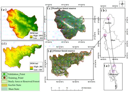
Figure 1.
Location of the study area: (a) country boundary; (b) location of the two forest reserves; (c) the Sentinel-2 true color image (collected in 26 January 2017) attached with field sample plots in NH; (d) the Sentinel-2 true color image (collected in 5 February 2017) attached with field sample plots in YM; (e) the DEM of NH; and (f) the DEM of YM.
The NH forest reserve area is approximately 19,418 hectares and the dense evergreen forest type dominates this region, geographically spanning from 97°13′00″E, 27°23′30″N to 97°24′30″E, 27°13′00″N. It is situated in the Putao Township, Myitkyina District, of northern Kachin State. The terrain in the region is mountainous, with an altitude ranging from 416 m to 1951 m. The annual average temperature of the area is 22.13 °C, with its average annual precipitation ranging from 1218 mm to 2800 mm; snowfall used to be heavy in the northern part, at higher altitudes of the mountainous regions. Evergreen tree species such as Quercus glauca, Macaranga denticulata, Michelia champaca, Shorea assamica, and Ficus cuspidata, are typical tree species of NH. A village called “Namhton Ku” is located in the center of this reserved forest as an encroachment, where forest-related field data collection was not performed.
The YM is a deciduous forest reserve-dominated region with an area of 20,163 hectares which is located between latitude 23°7′30″N–23°17′00″N and longitude 96°18′30″E–96°33′30″E, in Moemaik Township, Kyaukme District of Shan State. The mean annual temperature of this region is approximately 27 °C with an average annual rainfall ranging from 1000 mm to 1500 mm. The terrain is relatively flat, ranging from 128 m to 261 m according to the analysis of the SRTM DEM data. The vegetation in the YM region is predominantly Dipterocapaceae species such as Dipterocarpus alatus, Hopea odorata, Dipterocarpus tuberculatus, and Shorea obtuse. The vegetation in this area is mainly deciduous, losing its leaves during the dry season. Additionally, bush fires, which frequently occur during the dry season, further reduce the available foliage. Biomass or carbon stocks during the dry season months can therefore dramatically differ from those during the rainy season for the same area.
2.2. Data Collection and Processing Methods
2.2.1. Sentinel-2 Images Pre-Processing and Indices Extraction
The study site is located in two eco-regions (northern and central eastern) of Myanmar. Frequent rains and cloud contamination exist in the study sites, which highly restrict the availability of images collected in the peak season of vegetation growth (i.e., June–September). Therefore, two S-2 L1C MSI satellite images, with tile numbers of T47RLL and T46QHL acquired on 26 January 2017 and 5 February 2017, respectively, were downloaded from the European Space Agency. Available online: https://www.scihub.copernicus.eu (accessed 21 March 2022). These images are composed of 100 km2 tiles with UTM/WGS84 projection. The descriptive information of the images is summarized in Table 1. The atmospheric correction of the two S-2 L1C scenes was performed with the Sen2Cor plugin in SNAP software to reduce the atmospheric, adjacency, and slope effects [51]. In the process, TOA reflectance images were converted into surface reflectance images with aerosol-free and noise reduction. Then, all 20 m spectral bands were resampled to 10 m using the nearest neighbor strategy. Bands 1, 9, and 10 were not suitable for AGB estimation and excluded from the analysis [52]. The images and spectral response curves for a test vegetation pixel before and after atmospheric correction are shown in Figure 2.

Table 1.
Descriptive information of the images used in the analysis.
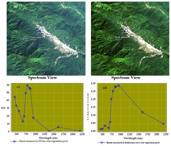
Figure 2.
The original Sentinel-2 L1C image (a) and atmospherically corrected image L2A (b), and the original (c) and corrected (d) spectral curves for a test vegetation pixel.
The individual application of spectral values in a predictive model could not give a reliable estimation compared to when using combined VIs. In addition to the spectral bands, VIs were calculated based on the original reflectance bands in the raster calculator tool. The plot-level vegetation index mean values were extracted using the zonal statistics tool of ArcGIS, and using the plot size (0.08 ha) to match the AGB calculations. In this study, the normalized difference vegetation index (NDVI) [53], red-edge normalized difference vegetation index (RENDVI) [54], weighted difference vegetation index (WDVI) [55], enhanced vegetation index (EVI) [56], red-edge enhanced vegetation index (REEVI) [57], soil-adjusted vegetation index (SAVI) [58], green-normalized vegetation index (GNDVI) [59], normalized difference water index (NDWI) [60], simple ratio (SR) [61], normalized difference vegetation index with bands 4 and 5 (NDI45) [62] and meris terrestrial chlorophyll index (MTCI) [63] were calculated. The detailed formulas for VIs calculation are described in Table 2.
Table 2.
List of Sentinel-2-derived variables and topographic factors used in AGB modeling.
2.2.2. SRTM Data Pre-Processing and Variables Extraction
SRTM topographic data were downloaded from the USGS EROS Data Center. Available online: https://www.earthexplorer.usgs.gov/ (accessed 23 March 2022). These elevation data offer worldwide coverage of void-filled data at a resolution of one arc-second (approximately 30 m) and a high-resolution global dataset. These topographic data were first reprojected into UTM/WGS84 since the projection system of these data are GCS/WGS84. To match with S-2 spectral bands, they were also resampled to 10 m spatial resolution using the nearest neighbor method in the ArcGIS package. Then, from this resampled dataset, two forest reserves boundaries were clipped and the elevation, slope and aspect were similarly extracted using the zonal statistics tool in ArcGIS (Table 2).
2.2.3. Texture Features Extraction
Principal component analysis (PCA) can be used to remove correlated or redundant information in the satellite images and simultaneously reduce their dimensionality [34]. The first three principal components were produced as the potential image variable for modeling AGB. The first principal component (PC1) was used for texture extraction as it contained over 80% of the original spectral information. When extracting textural features, the gray level co-occurrence matrix (GLCM) method and wavelet decomposition method were applied. Among these, the GLCM textures including the mean, variance, homogeneity, contrast, dissimilarity, entropy, second moment, and correlation were extracted with different window sizes (3 × 3, 5 × 5, 7 × 7) from the PC1 image in the ENVI5.3 package (Table 3). In this study, the GLCM-based textures derived from a 7 × 7 window size were selected as predictive variables for AGB estimation after the correlations of different window sizes’ textures with the measured AGB were tested.
Table 3.
Gray level co-occurrence matrix-based textural measures extracted in the current work.
Additionally, the wavelet analysis was also considered to be an effective means of extracting textures. Wavelet transformation is a multi-resolution analysis tool for image signal processing, which has two distinct abilities: subtle variation in spectral features in the original data can be detected at different scales and the useful information can be represented by fewer wavelet features by compressing data [51]. The wavelet analysis produces four basic components including the approximation image, horizontal detail, vertical detail and diagonal detail images of which the latter three are usually regarded as helpful textural measures. In this study, the Coiflect discrete wavelet function was chosen after repeated tests with different mother wavelets (the Haar wavelet, Daubechies (dbN) and Symlets (symN)) in the Matlab package because it had the highest correlation with AGB. Thus, based on the first principal component (PC1), a three-level decomposition strategy was implemented through programming in the Matlab environment to generate 9 detailed images as independent textural variables for AGB modeling. Finally, two types of textures derived from GLCM-based and wavelet analysis were included in the AGB modeling in this study. The Coiflet wavelet-based decomposition procedure is summarized in Figure 3.
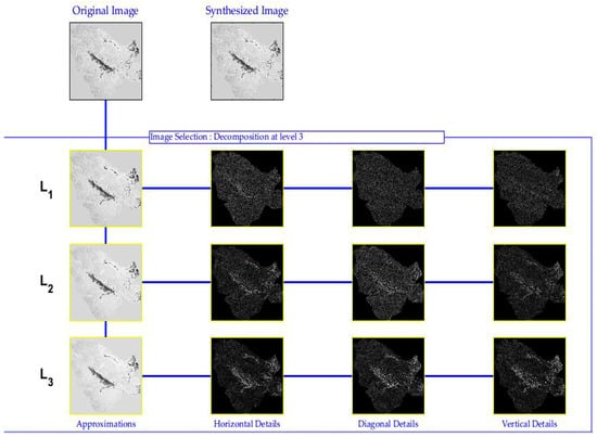
Figure 3.
Process of the Coiflect discrete wavelet decomposition for the PC1 of the original Sentinel-2 satellite images. L1–L3 is the decomposition level, and the first column shows the approximation images; the second column shows the images of horizontal details; the third column shows the images of diagonal details and the fourth column shows the images of vertical details.
2.2.4. Field Forest Inventory Data
Myanmar’s Forest Department conducted the national forest inventory (NFI) data collection in February and March of 2017 with the financial support of the Finnish government and according to the guidelines of the FAO technical team. These secondary forest inventoried data were used to estimate and infer the plot-level AGB of the study area. The sampling design of Myanmar’s NFI is shown in Figure 4. The systematic sampling method was constructed according to the eco-regions of Myanmar in order to cover all forest types. However, due to inaccessibility, no sample plots were collected for some areas in the NM (Figure 1c). Each sampling cluster comprises four 0.08-hectare circular subplots (Elbow, East, North and Northeast) in which the distance between adjacent subplots is 50 m. Within these circular subplots, all trees above 10 cm diameter at breast height (DBH) were measured to record data, including the DBH, tree height (H), and crown width. The diameter tape and Leica laser finder were used to measure the DBH and H of trees. Other forest parameters such as shrub cover, sapling cover, bamboo coverage, humus depth, litter coverage, and tree bark thickness were also collected in all sample plots. Ultimately, data collection was performed in 88 subplots in NH (evergreen forest) and 170 subplots in YM (deciduous forest).
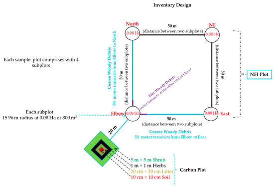
Figure 4.
Field forest inventory sampling design in Myanmar. Source: Planning and Statistics Division, Forest Department of Myanmar.
2.2.5. Allometric Equation and Calculated AGB
Since the species-specific allometric equations are not available for the study region, we had to use the unpublished national-level coarse allometric equations for evergreen forest and broad-leaved forest to calculate the plot-level AGB. The AGB formulas were as follows:
where, AGB is in kg per tree, DBH is in cm, ρ1 and ρ2 are the basic wood density parameters for evergreen forest and deciduous broad-leaved forest, respectively.
Using the national level biomass expansion factors Equations (1) and (2), AGB was computed for each tree and summed up by each plot to obtain plot-level AGB. Finally, the plot-level field AGB values were converted from kg/plot into ton/ha. Therefore, the AGB unit in this study was t/ha. Table 4 shows the descriptive statistics of the field-observed AGB.
Table 4.
Descriptive statistics of the field-measured AGB (t/ha) for the two forest reserves.
2.3. Aboveground Biomass Detection Methods
2.3.1. Prediction Model Establishment
In this study, Random Forest (RF) and stochastic gradient boosting (SGB) models were first performed for AGB prediction. Then, based on the better one (RF or SGB), the predicted residuals (the difference between the observed AGB and the model-predicted AGB) were further analyzed and compared using ordinary Kriging (OK) and the co-Kriging (CK) to separate the structured components hidden in the residuals, followed by adding the better structured components onto the better model predictions to obtain the final AGB predictions. The detailed modeling approaches are summarized as follows:
Random Forest and Stochastic Gradient Boosting Models
Parametric and non-parametric models have been utilized either alone or combined with environmental variables for remote sensing-based AGB mapping. Nevertheless, choosing the suitable variables set and modeling algorithm is critical for the improving the accuracy of prediction model.
The RF model is a bagging algorithm which enhances accuracy and reduces overfitting and bias [65]. SGB is a boosting ensemble method with low sensitivity to outliers, with the ability to deal with unbalanced training datasets [44]. Both models are non-parametric modeling approaches which have a performance superior to those of other machine learning techniques such as the K-nearest neighbor (KNN), support vector machine (SVM), and the multivariate adaptive regression splines (MARS) [66,67], which is increasingly being applied to satellite-based biomass mapping [9].
In view of these advantages, in the current study, the RF and SGB models were performed as the first attempt to predict the AGB of the two forest reserves (NH and YM). The RF model was implemented in the “randomForest” package [68] within R Studio. This package supports the chart that illustrates the GI-index and OOB error rate to determine the most important modeling variables. From this comprehensive chart, preference variables can be selected for a prediction model to reduce the complexity and load of computation. In the RF regression analysis, the variables’ importance ranking was determined by out-of-bag (OOB) error and node-purity percent (IncNodePurity). The first variable importance analysis was calculated by randomly permuting each predictor variable and computing the associated reduction in predictive performance using the out-of-bag (OOB) error. The second most important variable was estimated by determining the decrease in node impurities attributable to each predictor variable. Larger InNodePurity and %InMSE indicate higher model accuracy in terms of ranking variable importance. Parameters such as the number of trees (ntree), the number of variables used to split the tree at each node (mtry), and node size are adjustable for the RF model. For RF-prediction models in this study, after multiple tests, the ntree, mtry and nodesize were specified to be 600, 4, and 5 for the evergreen forest (NH) and 1400, 2, and 5 for the deciduous forest (YM), respectively.
The SGB algorithm is based on the combination of the regression tree and boosted algorithms to predict the response variable. This algorithm also reduces the chance of overfitting by introducing an element of stochasticity due to its flexibility and high predictive performance. Unlike RF, a tree is constructed from a different random sub-sample of the dataset in the SGB model, producing an incremental improvement in the model. In this study, all steps of the SGB analysis were implemented in the “gbm” package in the R-studio [69]. The “vip” function in the “gbm” package was also used for the selection of important variables for the SGB model. The SGB model adjustment includes the distribution, interaction depth, bagging fraction, shrinkage rate, and training fraction. The out-of-bag method was used for determining the optimal number of boosting iterations. The maximum iteration tree was stopped at 420 in the evergreen forest AGB (NH) SGB-prediction model and 600 at the deciduous forest AGB (YM) SGB-prediction model, as more iteration tree numbers could no longer improve models’ accuracy. The interaction depth, also known as the maximum number of possible interactions, was set to 3 and 4 nodes for the NH and YM SGB-models, respectively. The bagging fraction controlling the fraction of the training data, the shrinkage rate controlling the learning speed of the algorithm, and the training fraction randomly selected for calculating each tree were set to 10, 0.03, and 10 for both SGB models (NH and YM).
Once the RF and SGB models were created for the two forest reserves, their predictive performances in AGB estimation were compared to determine the better model; then, based on this model, all the residuals resulting from the model were further analyzed by implementing OK and CK autocorrelation algorithms to separate the structurized component or trend item hidden in the residuals.
Random Forest-Based Kriging Model
In this study, RF performed better than SGB in both the NH and YM AGB prediction models in terms of accuracy evaluations; thus, to improve the accuracy of RF models or finding the spatial correlation of AGB samples, RF-based OK and CK analyses (RFOK and RFCK) were also performed as subsequent steps. Since the RF model does not consider spatial autocorrelation among the AGB sample plots, AGB is actually a typical item with relatively high spatial autocorrelation; thus, a combination of RF and Kriging (RFK) was potentially an effective and more reliable means of determining the spatial distribution of AGB in this study. Specifically, a regression-Kriging technique was used to extract the structured components of the residuals obtained from the RF regression [70]. As the procedure of Kriging interpolation, the modeling semivariogram is important to determine the accuracy and reliability of the estimates. Kriging includes ordinary Kriging (OK) and co-Kriging (CK) in which OK is a suitable interpolation method for the uneven distribution of terrain and climatic variation events, while CK is the best method for improving the accuracy of target prediction [22]. OK is a linear estimation method suitable for inherently stationary random fields which satisfies the isotropic hypothesis [71] and fully considers spatial parametric non-stationarity as well as the effects of environmental variables derived from the benefits of RF. It is a widely used geostatistical technique that generates an optimal unbiased estimated surface employing a semivariogram based on regionalized variables. The interpolation formula of OK is as follows:
where ZOK * (x0) is the residual value of the AGB to be estimated at location 0, n is the number of sample points used for interpolation, Z) is the AGB residual of site , and is the weighting coefficient at point .
CK is an improvement over the OK method and deals with multivariate problems [22]. Since the study areas include two reserved forests with different terrains, AGB is definitely affected by elevation. Thus, the elevation factor was used as a co-variable for interpolation. This was expressed as follows:
where is the residual values of AGB to be estimated is the AGB residual of the site i, is the weighting coefficient of site i, is the elevation of site j, and is the weighting coefficient of site j.
Variograms are an effective tool for analyzing the spatial variation and structure of target predictors for the reliable estimation of AGB. The performance of the semivariogram was assessed by the coefficient of determination (R2) and the root mean square error (RMSE). The larger the R2, the smaller the RMSE and nugget effect, and the better the fitting performance was.
In RF-Kriging modeling, the estimated residual value of each sample point was calculated by subtracting the RF-derived predicted AGB value from the field-observed AGB value. It can be calculated as follows:
Final AGB prediction by RFOK or RFCK method was acquired by the following equation:
where is the predicted AGB at site i using RFOK or RFCK, where is the AGB residual value of site i, is the observed AGB of site i, is the RF-based predicted AGB at site i.
Finally, the maximum livelihood classifier in ENVI Classic 5.3 was applied to classify the forest and non-forest areas of the study area. The resulting classified forest area was used as a mask to obtain the forest AGB maps of the study area.
2.4. Accuracy Assessment
The training and validation sets were determined as 80 and 20% of the sampled data using stratified sampling for all statistical analyses. Model performances were assessed based on the coefficient of determination-R2, the mean absolute error (MAE), the root mean square error (RMSE), the RMSE%, bias, and bias%, based on the validation set (20% of samples). In addition, the relative improvement (RI) index for assessing RFOK and RFCK over RF models was also performed (7):
where, RMSERF is the root mean square error from RF predicted model, is the root mean square error from RFOK and RFCK models, respectively.
3. Results
3.1. Variable Importance and Selections
In the RF variable importance analysis, the %IncMSE by OOB error and %InNodePurity by Gini index are indicators of the importance ranking. The topmost important variables picked up by the evergreen NH and deciduous YM RF models are shown in Figure 5a,b. For the generalizing the model and reducing the computation load, only the top 10 variables were selected as the final RF model inputs. S-2 derived the reflectance, Vis and textures from the wavelet decomposition, and the topographic variables were included in the list. In the RF model, topographic variables and textures from WA were major contributors to the evergreen NH forest AGB estimation, while VIs showed better sensitivity to deciduous AGB.
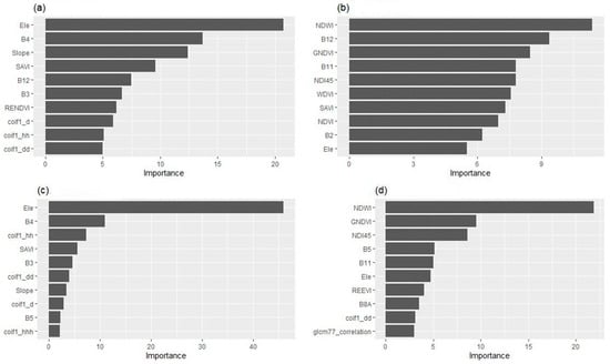
Figure 5.
The importance ranking of the top 10 variables identified by (a) evergreen RF model; (b) deciduous RF model; (c) evergreen SGB model; and (d) deciduous SGB model.
In the variables analysis for the SGB model, the lowest RMSE could be found for an interaction depth of 3, a shrinkage ratio of 0.03, and 420 iterations in the evergreen forest reserve. For the deciduous forest reserve, an interaction depth of 4, shrinkage ratio of 0.03, and 600 trees were the best parameters for model fitting. Figure 5c,d show the most important variables of SGB models for evergreen NH and deciduous YM AGB estimation. In SGB models, topographic variables and textures from WA were identified as major contributors to the NH evergreen AGB estimation, while VIs had better sensitivity for the deciduous AGB prediction. According to the variable importance analyses in the RF and SGB models, the variables did not differ a great deal in terms of their sensitivity to AGB in same forest types.
3.2. Validation Metrics for RF and SGB Models
Among the sample plots, 80% were used for training the models (RF and SGB). For the RF evergreen model training, the optimum model accuracy was obtained from the following parameters, ntree = 600, mtry = 4 with nodesize = 5, considering the important predictors. The adjusted parameters values of ntree = 1400, mtry = 2 and nodesize = 5 were selected for the RF deciduous model. The RMSEs values of 11.17, 17.36 t/ha and corresponding RMSE%s 23.06 and 17.45 were obtained while the R2 values were 0.95 and 0.97 for evergreen and deciduous training models. It was also observed that the bias and bias% of the evergreen training models were −0.59 and −1.20%, while the deciduous model obtained −0.011 and −0.11%, respectively. The smallest RMSE value was observed in the evergreen forest since the AGB values of the training plots in this type were smaller than those of the deciduous forest (Table 4).
Depending on the shrinkage ratio, the interaction depth, and the number of regression trees, the two SGB model performances were evaluated. The SGB evergreen model resulted in an R2 value of 0.98 and an RMSE of 4.62 t/ha with the corresponding RMSE%, bias and bias% of 9.45, −1.24 and −2.54, respectively. In the trained model of SGB for the deciduous forest, the R2, RMSE, RMSE%, bias and bias% were 0.97, 8.83, 8.88, −3.02 and −3.04.
In addition to model training, 20% of the sample plots were used for model validation. Figure 6 and Table 5 show the validation metrics for RF and SGB models. The R2 values of the NH evergreen RF model and NH SGB model were 0.47 and 0.35, respectively, while RMSEs values of those models were 25.45 and 32.02 t/ha, respectively. Meanwhile, the R2 and RMSE values of the YM deciduous RF model and YM SGB model were estimated to be 0.38, 0.35 and 40.23, 41.85 t/ha. In the scatter plots of Figure 6, the points along the fitted lines showing the correlation of predicted and observed AGB are scattered in both NH and YM, which showed large AGB values which were underestimated and small AGB values which were overestimated. Nevertheless, by considering the validation models’ metrics, the RF models had higher R2, lower RMSE, and bias values than SGB models in the biomass estimation at each growth stage, indicating that the RF models can provide more accurate biomass estimations than SGB; thus, the residuals from the RF model were further analyzed to attempt to extract the structured components from the residuals to possibly improve the ultimate prediction accuracy of AGB.
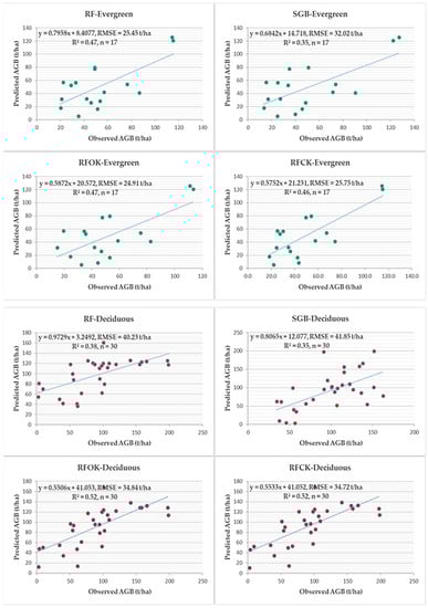
Figure 6.
The scatter plots for validation metrics of RF, SGB, RFOK, and RFCK models.
Table 5.
Validation metrics of RF, SGB, RFOK, and RFCK models based on 20% of the sampled data.
3.3. Semivariogram Analysis Results of RF-Derived Residuals
Residuals of the RF-predicted AGB were derived by subtracting the RF-predicted AGB from the field-measured AGB. Table 6 shows the statistics of the residuals. The mean residual values for the evergreen and deciduous AGB were −0.91 and −1.60 t/ha, respectively. In addition, the residual value range of the deciduous forest (82.43 t/ha) was much higher than that of the evergreen forest (34.52 t/ha). The standard deviation of the evergreen residuals (15.38 t/ha) was smaller than that of the deciduous (23.12 t/ha). The residual values were shown in different colors and sizes based on their distribution in Figure 7. As shown in the histogram distribution in Figure 7, the residual values of the evergreen forest were not close to normal distribution while deciduous residuals were approximately normally distributed. Nevertheless, the procedure of the semivariogram analyses for both forest reserves was performed for testing the accuracy of the models.
Table 6.
Residual’s statistics derived from the RF model prediction.
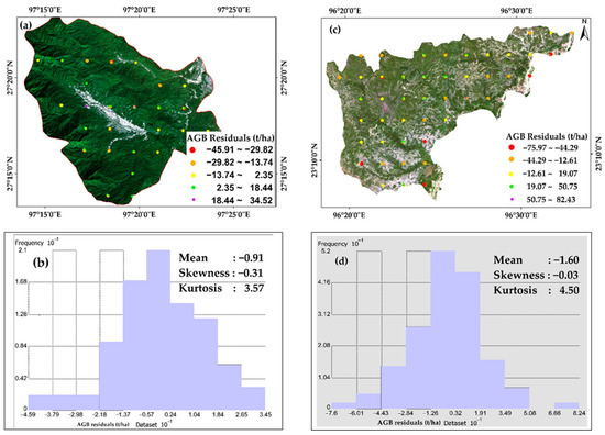
Figure 7.
Spatial distributions of the residuals and corresponding frequency histograms; (a,c) are RF-based AGB-residuals for NH evergreen and YM deciduous, respectively; (b,d) are frequency histograms of AGB-residuals for NH evergreen and YM deciduous, respectively.
After the normality of the residuals was verified in SPSS, these residual values could be used for semivariogram analysis based on the ordinary Kriging (OK) and the co-Kriging (CK) in the semivariance analysis. The model with the largest R2 and smallest RMSE was determined as the optimal analytical function of the semivariogram. As a result, Gaussian function was picked up (Table 7). Furthermore, elevation was used as a co-variable in the CK model for the better estimation of AGB. Table 7 and Figure 8 show the modeled semivariogram and semivariance models using OK and CK analyses. Evergreen forest models were poorly fitted; the R2 values were much lower than those of deciduous models (0.19-OK and 0.15-CK versus 0.58-OK and 0.62-CK). The nugget value in the OK model of the evergreen AGB residuals was slightly smaller than that of the corresponding CK model, indicating stronger spatial homogeneity. In the CK model of deciduous residuals, the nugget value was also smaller than that of the OK model. Moreover, the ratio of nugget and sill (nugget/sill) determined the variation of spatial autocorrelation between the AGB sample plots. From the OK models, the smaller nugget/sill ratio (0.95) exhibited stronger spatial homogeneity than the CK model with nugget/sill (0.99) for evergreen residuals. In the deciduous residuals, CK gave a smaller nugget/sill (0.74), indicating a stronger spatial correlation by considering elevation as a co-variable. This meant that deciduous forest AGB varied closely in space with the terrain variations. The improvement was not obvious in the evergreen OK and CK models compared to the evergreen RF model since the residuals were not normally distributed because of the existence of a spatial gap between the evergreen sample plots that restrict the principle of spatial correlation (Figure 7a). Thus, the OK model could not serve to fit the spatial patterns of the residuals in the evergreen forest AGB, while the CK model performed better in terms of fitting the spatial patterns of the residuals in the deciduous forest AGB in the study area when considering their R2 and RMSE values. Nevertheless, these residuals were used to interpolate their structured components in the evergreen and deciduous forests, respectively.
Table 7.
Parameter estimations for the semivariogram analysis based on Gaussian function.
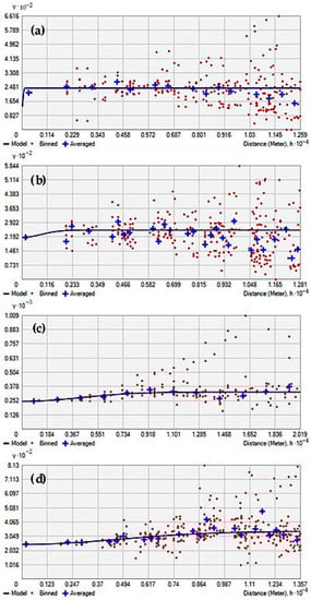
Figure 8.
Empirical semivariograms and covariance models for the two forest reserves’ RF-derived residuals; (a,c) are the semivariogram models for NH evergreen and YM deciduous using OK analysis; (b,d) are the semivariogram models for NH evergreen and YM deciduous using CK analysis with a covariable of elevation. The vertical axis is the ½ variance (γ) and covariance (C) of the two positions as the distance increases.
3.4. Forest AGB Mapping Results Based on RFOK and RFCK Models
The predicted AGB of the two forest reserves were obtained from the RFOK for the evergreen and RFCK for the deciduous forests, and the validation performances with 20% sample data based on Equation (6) were correspondingly derived. Table 5 shows the validation accuracy improvements of RFOK and RFCK in relation to the initial RF model.
Although the R2 value (0.47) of the RFOK model for evergreen did not increase compared to the original RF model, its RMSE, RMSE% and MAE all decreased with different magnitudes, and its RI value was 0.02, indicating a slight improvement in AGB prediction. However, the RFOK had the worst predictive performance in the evergreen forest. For the deciduous forest, the RFCK model outperformed other two RFOK and RF models, particularly in relation to the RF, as the RFCK’s R square value increased from 0.38 to 0.52 and its RMSE decreased from 40.23 t/ha to 34.72 t/ha, with an RI value of 13.7%. However, compared to RFOK, RFCK only took on a very tiny improvement in the prediction accuracy.
In addition to the model evaluation, the generalization ability of the model was also considered. The AGB value range of the predicted map could reflect the model’s robustness to some extent. The range of AGB values predicted for the evergreen using the RF model was 88.75–129 t/ha. The AGB prediction value range from RFOK was 94.3–139.83 t/ha and the RFCK had a value range of 94.06–139.62 t/ha, respectively. The AGB prediction value range in the deciduous was 40–176 t/ha, 30.41–187.84 t/ha, and 32.88–185.65 t/ha for RF, RFOK, and RFCK. These variations in the value range clearly indicated an improved generalization ability of RFOK and RFCK, with higher robustness. The largest evergreen AGB values were found in the northern and western boundaries of NH while the AGB in the central and eastern parts were sparsely distributed. In this area, the low AGB values were found close to a village and flat area. Deciduous AGB was covered with large values in some parts of northern YM, and they were evenly distributed in the reserved area, except in the southeastern boundary which is close to a village. The AGB maps derived from all performed models are shown in Figure 9 and Figure 10.
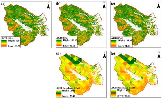
Figure 9.
The estimated AGB of evergreen forests in the NM from (a) RF, (b) RFOK, and (c) RFCK models, and the calculated residuals for (d) RFOK and (e) RFCK models.
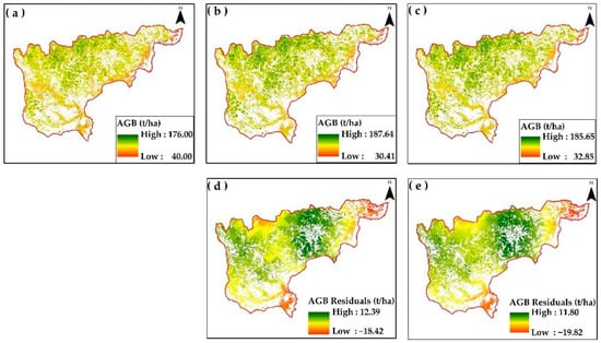
Figure 10.
The estimated AGB of deciduous forests in the YM from (a) RF, (b) RFOK, and (c) RFCK models, and the calculated residuals for (d) RFOK and (e) RFCK models.
4. Discussions
To the best of our knowledge, this is the first study evaluating the capability of S-2 satellite data for AGB mapping in evergreen and deciduous forest reserves in Myanmar. AGB mapping in these forest reserves is very fundamental for carbon strategies, especially for Myanmar REDD+ mechanisms which need to report the carbon improvement of forests from reforestation programs for future FREL submission. Moreover, the prediction methods proposed in this study are noticeably relevant for future forest management practices in Myanmar, which previously exhibited a lack of robust AGB estimation methods for forest types. We proved that THE combined use of S-2, its derivatives, and topographic parameters, in tandem with proper modeling techniques, could improve AGB estimation.
4.1. Sensitivity of Sentinel-2 Derivatives to AGB
The correct selection of variables contributing to a model is critical for AGB estimation. In most AGB mapping studies with S-2 derivatives, four novel wavebands in the red-edge region and near-infrared region (NIR) (B5, B6, B7 and B8A) showed good performance [16,72]. These reflectance regions offer unprecedented spectral signatures which are highly sensitive to the biophysical and biochemical responses of vegetation that are critical for measuring vegetation characteristics such as biomass [72]. However, in this study, the classical and short-wave infrared bands (B2, B3, B4, B11, and B12) outperformed these aforementioned spectral bands. The excellent performance of these bands is that carbon and nitrogen-containing metabolites reach their reflectance peak in wavebands between 440 nm and 570 nm due to the nature of the forests in the study area (B2 and B3) and concurred with the previous study [73]. Forest canopy in the evergreen forest can uptake maximum chlorophyll absorption due to non-deciduous phenomena. B3 and B4 in the S-2 have strong sensitivity to chlorophyll in evergreen vegetation, while B2 can effectively distinguish vegetation and soil background in the deciduous forest where the reflectivity of soil is apparent because of the simple canopy structure. Even though vegetation can reflect the maximum energy at NIR despite the fact that it is unable to provide any information on the soil under the vegetation, SWIR bands in S-2 can distinguish the vegetation and soil to some extent. A recent finding by Chen et al. verified that SWIR spectral bands (B11) could efficiently detect the moisture content of vegetation [37]. Moreover, Dang et al. proved that the broad bands (B11, B12) of S-2 were the best response variables of AGB prediction with an R2 of 0.81 and an RMSE of 36.67 Mg t/ha [6]. Hence, the high sensitivity of SWIR bands to biomass observed in this study seems plausible, which is in agreement with the existing studies.
The VIs used in this study (NDVI, GNDVI, SAVI, SR, RENDVI, NDI45, and NDWI) were primary contributors to the AGB estimation of forests since they have the ability to maximize the sensitivity of vegetation characteristics and minimize soil background reflectance and atmospheric effects. Balidoy et al. proved that the SR and NDVI of S-2 data were the most effective biomass predictors, providing the highest accuracy (R2 = 0.89; RMSE = 5.69 Mg/ha) [74]. Ghosh et al. found that the effectiveness of NDVI, GNDVI, SAVI indices of S-2 for dense tropical AGB mapping had an R2 value of 0.6 and an RMSE value of 79.45 t/ha for the teak forest [35]. The findings of Pandit et al. were entirely consistent with those of this study. The set of 24 variables including NDVI, GNDVI, RENDVI, SAVI, and SR produced overall plausible and strongly explained variable values, with R2 = 0.81 and RMSE = 1.07 kg/m [72]. Although VIs produced from traditional broad bands can reduce the saturation problem in simple canopy forest, they are less sensitive to complex forest stands with high biomass values [75]. In this regard, the red-edge bands derived indices are highly sensitive to such kind of dense vegetation structures and relatively less prone to spectral saturation. For example, the standard NDVI from B4 and B8 is less effective than RENDVI from red-edge bands (B5, B8) in AGB estimation [76] and hence red-edge-derived indices can be effectively applied in dense vegetation cover (e.g., RENDVI is sensitive to the NH evergreen forest AGB in the current work). SWIR bands are related with nitrogen, lignin, and cellulose, capable of retrieving canopy structural attributes and biomass. Canopy water content index from SWIR bands (e.g., NDWI in this work) is highly sensitive to deciduous forest AGB but not to evergreen AGB because canopy structure in deciduous forest is relatively simple, which is in agreement with the previous findings of Ewald [77]. They pointed out that in the very dense canopy plantation, SWIR indices could not effectively improve AGB estimation compared to other indices. This study claims that red-edge indices are suitable for complex canopy AGB retrievals while SWIR indices are useful for simple canopy forest AGB estimation.
The textural variables are strongest candidates of evergreen forest AGB, especially the textures (coif1-d, coif1-dd, and coif1-hh) extracted from Coiflect wavelet analysis of the PC1 image. They could obviously improve the AGB estimation as the horizontal structures of the evergreen forest can be effectively characterized by them. Previous research had shown that texture measures have the potential to improve AGB estimation, especially for complex vegetation structures where canopies’ reflectance values tend to be saturated but the horizontal structures represented by textural indices still have differences. If proper processing techniques are used, textural measures could improve the prediction accuracy of AGB models. According to Eckert et al., textures were much better to capture the various forest canopy structures of the forest strata than the spectral reflectance or band ratios, due to their sensitivity to the spatial aspects of the canopy shadow [78]. Su et al. proved the excellent performance of textures from the PC1 image for AGB prediction of sub-tropical forest where saturation problem occurred [22]. Moreover, Cutler et al. argued that the textures extracted from GLCM method and the WA of satellite images yielded better results in the AGB estimation and forest type classification [79]. Our results concur with aforementioned studies. However, in this study, GLCM-based textures were not highly correlated with AGB. The reason might be that the window size (7 × 7) could not reduce the border effects of pixels to attain original spectral values and thus, texture window size determination should be considered in accordance with the types of satellite data in future studies. We conclude that the wavelet decomposition analysis of satellite images might improve evergreen forest AGB estimation because it produces more suitable textures to effectively depict evergreen forest horizontal structures to reduce the saturation problem of spectral signals.
4.2. Sensitivity of Topographic Variables to AGB
Topographic features (elevation and slope) were also strong predictors of AGB in this study. The vital role of topography is also an important factor influencing AGB because water and sunlight storage change in function of topography [80]. Chen et al. proved that elevation was the strongest factor for complex AGB estimation in China [37]. Slope inclination was also a strong factor affecting AGB in the evergreen forest, since the terrain in this area is mountainous with different sunlight and water detention levels by its varying geomorphological characteristics while deciduous forest is not affected by slope by growing its trees over sandy soil flat surface. This finding is consistent with the proof of Hamere et al., which claimed that AGB carbon, BGB carbon, and the total carbon density trend showed a decrease as the slope increased due to the little vegetation cover in very steep slope areas [81]. In addition, in the accessible flat area of nearby settlements and stream banks, the anthropogenic effects might decrease AGB values. Therefore, topographic factors ultimately affect the AGB observed in this study.
4.3. Comparison between Models
This study evaluated the two modeling techniques (RF and SGB) for AGB mapping in two forest reserves and indicated a saturation problem of S-2 d satellite data, thus causing the presence of bias in the AGB prediction models. The NH evergreen RF model estimated the smaller AGB value of 129 t/ha than the observed AGB value of 151.64 t/ha. Similarly, the estimation of the YM deciduous forest AGB value (176 t/ha) was smaller than the field-observed AGB value (215.24 t/ha). The scatterplots in the validation metrics of this study indicated the limitation of the classical wavelength bands in the S-2 MSI sensor when dealing with saturation in high biomass stands. From the important variables ranking, the candidates of the classical wavelength region and topography such as B3, B4, Ele, Slope, and one vegetation index SAVI in the evergreen forest, and B11, B12, NDWI, and GNDVI in the deciduous forest were high ranked while no red-edge reflectance was correlated with AGB. This ranking affects the performance of models since the improvement in red-edge bands features was relatively larger than that in classical bands and topographic variables. This assumption was proven by previous studies of Forkuor et al. [76] and Nuthammachot et al. [30]. Additionally, Chen et al. suggested that the broadleaved forests with AGB values above 160 t/ha could be underestimated because of the saturation problem in S-2 satellite data [82]. The observed AGB value in the YM deciduous forest was 215.24 t/ha and thus should agree with the finding of Chen. An almost similar ranking in variables was observed in the two SGB models but the two models could not improve the estimation when considering their performances in prediction. Thus, these SGB models occurred and similar saturation problem was found in the RF models.
In order to optimize the estimation, the Kriging interpolation analysis of the residuals from RF models (RFK) was further employed since the RF showed better performance than SGB in this study. Our study claimed that the ordinary Kriging of RF’s residuals (RFOK) performed better than other tested models in NH evergreen, while co-Kriging of RF’s residuals (RFCK) with covariance elevation (Ele) provides a better result than other models in YM deciduous AGB prediction. The limited contribution of the accuracy of the RFOK model for the NH evergreen forest reserve was due to the poor spatial autocorrelation between AGB samples which occurred due to the spatial gaps between the sample plots. In the YM deciduous forest, RFCK achieved good prediction results, however, the spatial correlations of the current AGB were also weaker than previous studies of Su et al. and Chen et al. on forest AGB mapping based on the integration of multi-sensor and Advanced Land Observing Satellite (ALOS) data [22,37]. It was denoted that AGB residuals from the integration of the MSI and SRTM data model in this study obtained a lower spatial correlation than that built by the integration of MSI and ALOS indices. This also proves that AGB estimation from the combined MSI and SRTM data was only suitable for the simple structure forest stand (e.g., deciduous forest in this study).
Overall, we conclude that the accuracies of AGB prediction could be improved to a certain extent by Kriging methods by reducing the spatial heterogeneity between AGB samples. In the future, the accuracy of evergreen forest AGB estimation in this study might be improved with LiDAR data since it can penetrate the forest canopy to a certain depth, so that its variables are suitable for extracting vertical vegetation structures with their sensitivity to the biomass of vegetation and the roughness of land cover surfaces. The determinant of the spatial setting and a sufficient number of sample plots should be considered in future AGB studies to maintain the Kriging accuracy. Additionally, the study area is located in the regions where frequent rains and clouds exists, highly restricting the availability of images collected in the vegetation growth peak season (e.g., June–September). Therefore, we had to use cloud-free images acquired in January or February, which falls outside the ideal time window for characterizing vegetation attributes. This limitation may affect the accuracy of forest AGB prediction model.
In addition, an allometric equation for in situ AGB calculation may be another factor undermining accuracy. This study used a national-level coarse allometric equation which was based on an existing inventory dataset and pantropical equation (Chave et al., 2005, Chen et al., 2013, and IPCC, 2003) for AGB calculation since there have been no species-specific equations developed for this study area. In the near future, developing species-specific allometric equations through limited destructive sampling should prioritize the carbon accounting and climate change response studies in Myanmar because these create more accurate in situ plot-level AGB measurements, laying a solid foundation for the remote sensing-based regional estimation of AGB. In general, AGB estimated from the RF model could yield acceptable results of validated R2 = 0.47, RMSE = 25.45 t/ha for evergreen and R2 = 0.38, RMSE= 40.23 t/ha for deciduous from S-2 derivatives, topographic variables and ancillary information.
4.4. Effects of Forest Management on AGB in the Study Sites
Population growth has led to a high demand for forest products, unsustainable forest management practices, and high deforestation rates, thus causing forest cover loss. The extent of the forest cover loss depends on the forest protection status with different rules applying to public and reserved areas [83]. Forest protection typically reduces the conversion of natural land cover types to alternative uses and often results in positive outcomes (including reduced deforestation rates and the maintenance of forest cover) compared to unprotected sites. In Myanmar, intact forests are gradually decreasing to only 38% of the country’s forests due to the rapid political and economic changes. The study site comprises two protected forests under Myanmar forest law. However, the expansion of the human population and the need for more agricultural lands tend to encroach into these areas, especially in the evergreen forest presently under study. Encroachment in protected forests for agricultural lands, food, and fuels is directly correlated with loss in AGB values. On the other hand, deciduous forests’ AGB values might be following a decreasing trend because the demands for commercial timber species are increasing and AGB sources are gradually decreasing. In this context, the spatial agreement of AGB was observed in the estimated AGB maps derived from the RFOK evergreen and RFCK deciduous models. For example, the small AGB values were estimated in the forest area closest to the villages and cultivated lands while large AGB values were distributed in the high-elevation forest of the NH evergreen forest reserve. A similar finding was observed in the YM deciduous forest. To sustain the forest AGB in these areas, community-based forest management is suggested to reduce these pressures as this would meet the needs of forestry products for forest dwellers.
4.5. Attainment for SDG and REDD+
The UN SDGs set out the commitment of the international community to rid the world of poverty and hunger and achieve sustainable development in its three dimensions—the economic, social and environmental facets. In addition to using standardized national official data sources as the basis for monitoring and reporting on these goals and targets, geospatial information and global/regional datasets have been identified as viable replacement and complementary data sources for achieving these SDGs [84]. As the indicator of SDG 15, the accurate estimation and monitoring of aboveground biomass stocks need to be achieved. In this regard, the results of this study are applicable and useful for the attainment of SDG 15, especially for Myanmar where freely available optical data are preferred to map biomass stocks, and will greatly assist in the deriving, monitoring, and reporting of carbon stock changes in a timely and accurate manner.
Myanmar has been implementing the REDD+ project to achieve SDG goals and targets through sustainable forest management practices since 2013. The REDD+ objective is to find an accurate method of biomass estimation that is also cost-effective. Based on the results obtained in this study, S-2-derived derivatives (spectra, VIs, textures) and the topographic features of SRTM (elevation, slope) have potential in the forest biomass estimation of two forest reserves. In addition, the methods used in this study are viable and compatible software has been developed (e.g., SNAP), in such a way that REDD+ can apply it at a larger scale, including the national and regional levels. The outcomes of this study can surely assist the evaluation of carbon stock changes via reforestation programs that will be included in the upcoming FREL calculation under the REDD+ agenda of Myanmar.
5. Conclusions
This study investigates the performance of S-2 MSI derivatives and SRTM DEM topographic data with field ancillary information based on two machine learning models (RF and SGB) in mapping the forest AGB of two forest reserves (namely the NH evergreen and YM deciduous forests) in Myanmar. In addition, the RF-based Kriging (RFK) was employed for improving the prediction accuracy to find a spatial correction between the AGB samples. Based on these findings, it is concluded that:
- (1)
- S-2-derived reflectance, VIs, and textures are effective in predicting the AGB of the two forests if the proper processing techniques are applied;
- (2)
- The RFOK model in the evergreen forest and RFCK model in the deciduous forest provided a more realistic spatial distribution of AGB by considering the spatial correlation than the RF and SGB models with R2 = 0.47, RMSE = 24.91 t/ha and R2 = 0.52, RMSE = 34.72 t/ha due to their spatial correlation between AGB sample plots;
- (3)
- The extraction of textures from wavelet analysis (WA) is suggested to improve estimation for the forests with a complex structure and saturation problems;
- (4)
- In future studies, the accuracy may be improved by combining both the active and passive remotely sensed data to characterize complex forest structures to better estimate the forest AGB and understand their spatial distributions.
Author Contributions
Conceptualization, M.L.; methodology, P.W. and H.S.; software, P.W. and H.S.; validation, P.W. and H.S.; formal analysis, P.W.; investigation, P.W.; resources, M.L. and P.W.; data curation, P.W. and H.S.; writing—original draft preparation, P.W.; writing—review and editing, M.L.; visualization, P.W.; supervision, M.L.; project administration, M.L.; funding acquisition, M.L. All authors have read and agreed to the published version of the manuscript.
Funding
This research was jointly funded by the Natural Science Foundation of China, grant number 31971577, the Priority Academic Program Development of Jiangsu Higher Education Institutions (PAPD).
Data Availability Statement
Not applicable.
Acknowledgments
Special thanks need to go to the European Space Agency for the provision of the remotely sensed images used in the work and the Forest Department of Myanmar for providing the forest inventory data.
Conflicts of Interest
The authors declare no conflict of interest.
References
- Bonan, G.B. Forests and Climate Change: Forcings, Feedbacks, and the Climate Benefits of Forests. Science 2008, 320, 1444–1449. [Google Scholar] [CrossRef] [PubMed] [Green Version]
- Wolosin, M.; Harris, N. Tropical Forests and Climate Change: The Latest Science; World Resources Institute: Washington, DC, USA, 2018. [Google Scholar]
- Rodríguez-Veiga, P.; Wheeler, J.; Louis, V.; Tansey, K.; Balzter, H. Quantifying Forest Biomass Carbon Stocks from Space. Curr. For. Rep. 2017, 3, 1–18. [Google Scholar] [CrossRef] [Green Version]
- Gibbs, H.K.; Brown, S.; Niles, J.O.; Foley, J.A. Monitoring and Estimating Tropical Forest Carbon Stocks: Making REDD a Reality. Environ. Res. Lett. 2007, 2, 045023. [Google Scholar] [CrossRef]
- Basuki, T.M.; van Laake, P.E.; Skidmore, A.K.; Hussin, Y.A. Allometric Equations for Estimating the Above-Ground Biomass in Tropical Lowland Dipterocarp Forests. For. Ecol. Manag. 2009, 257, 1684–1694. [Google Scholar] [CrossRef]
- Dang, A.T.N.; Nandy, S.; Srinet, R.; Luong, N.V.; Ghosh, S.; Senthil Kumar, A. Forest Aboveground Biomass Estimation Using Machine Learning Regression Algorithm in Yok Don National Park, Vietnam. Ecol. Inform. 2019, 50, 24–32. [Google Scholar] [CrossRef]
- Lu, D.; Chen, Q.; Wang, G.; Liu, L.; Li, G.; Moran, E. A Survey of Remote Sensing-Based Aboveground Biomass Estimation Methods in Forest Ecosystems. Int. J. Digit. Earth 2016, 9, 63–105. [Google Scholar] [CrossRef]
- Li, Y.; Li, M.; Li, C.; Liu, Z. Forest Aboveground Biomass Estimation Using Landsat 8 and Sentinel-1A Data with Machine Learning Algorithms. Sci. Rep. 2020, 10, 9952. [Google Scholar] [CrossRef] [PubMed]
- Shen, W.; Li, M.; Huang, C.; Tao, X.; Wei, A. Annual Forest Aboveground Biomass Changes Mapped Using ICESat/GLAS Measurements, Historical Inventory Data, and Time-Series Optical and Radar Imagery for Guangdong Province, China. Agric. For. Meteorol. 2018, 259, 23–38. [Google Scholar] [CrossRef] [Green Version]
- Mon, M.S.; Myint, A.A. Estimating above Ground Biomass of Tropical Mixed Deciduous Forests Using Landsat ETM+ Imagery for Two Reserved Forests in Bago Yoma Region, Myanmar. In Proceedings of the Multi-Scale Forest Biomass Assessment and Monitoring in the Hindu Kush Himalayan Region: A Geospatial Perspective; Murthy, M.S.R., Wesselman, S., Gilani, H., Eds.; International Centre for Integrated Mountain Development: Patan, Nepal, 2015; pp. 165–177. [Google Scholar]
- Madugundu, R.; Nizalapur, V.; Jha, C.S. Estimation of LAI and Above-Ground Biomass in Deciduous Forests: Western Ghats of Karnataka, India. Int. J. Appl. Earth Obs. Geoinf. 2008, 10, 211–219. [Google Scholar] [CrossRef]
- Naveenkumar, J.; Arunkumar, K.S.; Sundarapandian, S. Biomass and Carbon Stocks of a Tropical Dry Forest of the Javadi Hills, Eastern Ghats, India. Carbon Manag. 2017, 8, 351–361. [Google Scholar] [CrossRef]
- Gasparri, N.I.; Parmuchi, M.G.; Bono, J.; Karszenbaum, H.; Montenegro, C.L. Assessing Multi-Temporal Landsat 7 ETM+ Images for Estimating above-Ground Biomass in Subtropical Dry Forests of Argentina. J. Arid Environ. 2010, 74, 1262–1270. [Google Scholar] [CrossRef]
- Li, M.; Tan, Y.; Pan, J.; Peng, S. Modeling Forest Aboveground Biomass by Combining Spectrum, Textures and Topographic Features. Front. For. China 2008, 3, 10–15. [Google Scholar] [CrossRef]
- Shen, W.; Li, M.; Huang, C.; Wei, A. Quantifying Live Aboveground Biomass and Forest Disturbance of Mountainous Natural and Plantation Forests in Northern Guangdong, China, Based on Multi-Temporal Landsat, PALSAR and Field Plot Data. Remote Sens. 2016, 8, 595. [Google Scholar] [CrossRef] [Green Version]
- Castillo, J.A.A.; Apan, A.A.; Maraseni, T.N.; Salmo, S.G. Estimation and Mapping of Above-Ground Biomass of Mangrove Forests and Their Replacement Land Uses in the Philippines Using Sentinel Imagery. ISPRS J. Photogramm. Remote Sens. 2017, 134, 70–85. [Google Scholar] [CrossRef]
- Xue, B. Lidar and Machine Learning Estimation of Hardwood Forest Biomass in Mountainous and Bottomland Environments. Master’s Thesis, University of Arkansas, Fayetteville, AR, USA, 2015. [Google Scholar]
- Pham, T.D.; Yokoya, N.; Bui, D.T.; Yoshino, K.; Friess, D.A. Remote Sensing Approaches for Monitoring Mangrove Species, Structure, and Biomass: Opportunities and Challenges. Remote Sens. 2019, 11, 230. [Google Scholar] [CrossRef] [Green Version]
- Laurin, G.V.; Chen, Q.; Lindsell, J.A.; Coomes, D.A.; Del Frate, F.; Guerriero, L.; Pirotti, F.; Valentini, R. Above Ground Biomass Estimation in an African Tropical Forest with Lidar and Hyperspectral Data. ISPRS J. Photogramm. Remote Sens. 2014, 89, 49–58. [Google Scholar] [CrossRef]
- Yuan, X.; Li, L.; Tian, X.; Luo, G.; Chen, X. Estimation of Above-Ground Biomass Using MODIS Satellite Imagery of Multiple Land-Cover Types in China. Remote Sens. Lett. 2016, 7, 1141–1149. [Google Scholar] [CrossRef]
- Blackard, J.A.; Finco, M.V.; Helmer, E.H.; Holden, G.R.; Hoppus, M.L.; Jacobs, D.M. Mapping US Forest Biomass Using Nationwide Forest Inventory Data and Moderate Resolution Information. Remote Sens. Environ. 2008, 112, 1658–1677. [Google Scholar] [CrossRef]
- Su, H.; Shen, W.; Wang, J.; Ali, A.; Li, M. Machine Learning and Geostatistical Approaches for Estimating Aboveground Biomass in Chinese Subtropical Forests. For. Ecosyst. 2020, 7, 64. [Google Scholar] [CrossRef]
- López-Serrano, P.M.; Cárdenas Domínguez, J.L.; Corral-Rivas, J.J.; Jiménez, E.; López-Sánchez, C.A.; Vega-Nieva, D.J. Modeling of Aboveground Biomass with Landsat 8 OLI and Machine Learning in Temperate Forests. Forests 2019, 11, 11. [Google Scholar] [CrossRef] [Green Version]
- Addabbo, P.; Focareta, M.; Marcuccio, S.; Votto, C.; Ullo, S.L. Contribution of Sentinel-2 Data for Applications in Vegetation Monitoring. Acta IMEKO 2016, 5, 44–54. [Google Scholar] [CrossRef]
- Gascon, F.; Ramoino, F.; Deanos, Y. Sentinel-2 Data Exploitation with ESA’s Sentinel-2 Toolbox. EGU Gen. Assem. 2017, 19, 19548. [Google Scholar]
- Imran, A.B.; Khan, K.; Ali, N.; Ahmad, N.; Ali, A.; Shah, K. Narrow Band Based and Broadband Derived Vegetation Indices Using Sentinel-2 Imagery to Estimate Vegetation Biomass. Glob. J. Environ. Sci. Manag. 2020, 6, 97–108. [Google Scholar] [CrossRef]
- Li, H.; Kato, T.; Hayashi, M.; Wu, L. Estimation of Forest Aboveground Biomass of Two Major Conifers in Ibaraki Prefecture, Japan, from PALSAR-2 and Sentinel-2 Data. Remote Sens. 2022, 14, 468. [Google Scholar] [CrossRef]
- Safari, A.; Sohrabi, H. Integration of Synthetic Aperture Radar and Multispectral Data for Aboveground Biomass Retrieval in Zagros Oak Forests, Iran: An Attempt on Sentinel Imagery. Int. J. Remote Sens. 2020, 41, 8069–8095. [Google Scholar] [CrossRef]
- Adamu, B.; Ibrahim, S.; Rasul, A.; Whanda, S.J.; Headboy, P.; Muhammed, I.; Maiha, I.A. Evaluating the Accuracy of Spectral Indices from Sentinel-2 Data for Estimating Forest Biomass in Urban Areas of the Tropical Savanna. Remote Sens. Appl. Soc. Environ. 2021, 22, 100484. [Google Scholar] [CrossRef]
- Nuthammachot, N.; Askar, A.; Stratoulias, D.; Wicaksono, P. Combined Use of Sentinel-1 and Sentinel-2 Data for Improving above-Ground Biomass Estimation. Geocarto Int. 2022, 37, 366–376. [Google Scholar] [CrossRef]
- Taddese, H.; Asrat, Z.; Burud, I.; Gobakken, T.; Ørka, H.O.; Dick, Ø.B.; Næsset, E. Use of Remotely Sensed Data to Enhance Estimation of Aboveground Biomass for the Dry Afromontane Forest in South-Central Ethiopia. Remote Sens. 2020, 12, 3335. [Google Scholar] [CrossRef]
- Li, L.; Zhou, X.; Chen, L.L.; Chen, L.L.; Zhang, Y.; Liu, Y. Estimating Urban Vegetation Biomass from Sentinel-2A Image Data. Forests 2020, 11, 125. [Google Scholar] [CrossRef] [Green Version]
- Pandit, S.; Tsuyuki, S.; Dube, T. Exploring the Inclusion of Sentinel-2 MSI Texture Metrics in above-Ground Biomass Estimation in the Community Forest of Nepal. Geocarto Int. 2019, 35, 1832–1849. [Google Scholar] [CrossRef]
- Jolliffe, I.T.; Cadima, J.; Cadima, J. Principal Component Analysis: A Review and Recent Developments. Philos. Trans. R. Soc. A Math. Phys. Eng. Sci. 2016, 374, 20150202. [Google Scholar] [CrossRef] [PubMed]
- Ghosh, S.M.; Behera, M.D. Aboveground Biomass Estimation Using Multi-Sensor Data Synergy and Machine Learning Algorithms in a Dense Tropical Forest. Appl. Geogr. 2018, 96, 29–40. [Google Scholar] [CrossRef]
- Ouma, Y.O.; Tetuko, J.; Tateishi, R. Analysis of Co-occurrence and Discrete Wavelet Transform Textures for Differentiation of Forest and Non-forest Vegetation in Very-high-resolution Optical-sensor Imagery. Int. J. Remote Sens. 2008, 29, 3417–3456. [Google Scholar] [CrossRef]
- Chen, L.; Wang, Y.; Ren, C.; Zhang, B.; Wang, Z. Optimal Combination of Predictors and Algorithms for Forest Above-Ground Biomass Mapping from Sentinel and SRTM Data. Remote Sens. 2019, 11, 414. [Google Scholar] [CrossRef] [Green Version]
- Wang, Y.; Zhang, X.; Guo, Z. Estimation of Tree Height and Aboveground Biomass of Coniferous Forests in North China Using Stereo ZY-3, Multispectral Sentinel-2, and DEM Data. Ecol. Indic. 2021, 126, 107645. [Google Scholar] [CrossRef]
- Simard, M.; Zhang, K.; Rivera-Monroy, V.H.; Ross, M.S.; Ruiz, P.L.; Castañeda-Moya, E.; Twilley, R.R.; Rodriguez, E. Mapping Height and Biomass of Mangrove Forests in Everglades National Park with SRTM Elevation Data. Photogramm. Eng. Remote Sens. 2006, 72, 299–311. [Google Scholar] [CrossRef]
- Ahmad, A.; Gilani, H.; Ahmad, S.R. Forest Aboveground Biomass Estimation and Mapping through High-Resolution Optical Satellite Imagery—A Literature Review. Forests 2021, 12, 914. [Google Scholar] [CrossRef]
- Zhang, J.; Lu, C.; Xu, H.; Wang, G. Estimating Aboveground Biomass of Pinus Densata-Dominated Forests Using Landsat Time Series and Permanent Sample Plot Data. J. For. Res. 2019, 30, 1689–1706. [Google Scholar] [CrossRef]
- Ye, Q.; Yu, S.; Liu, J.; Zhao, Q.; Zhao, Z. Aboveground Biomass Estimation of Black Locust Planted Forests with Aspect Variable Using Machine Learning Regression Algorithms. Ecol. Indic. 2021, 129, 107948. [Google Scholar] [CrossRef]
- Torres, C.; Almeida, D.; Soares, L.; Eduardo, L.; Cruz, D.O.; Pierre, J.; Balbaud, H.; Daniele, A.; Rocha, F.; Pereira, D.S.; et al. Combining LiDAR and Hyperspectral Data for Aboveground Biomass Modeling in the Brazilian Amazon Using Di Ff Erent Regression Algorithms. Remote Sens. Environ. 2019, 232, 111323. [Google Scholar] [CrossRef]
- Breiman, L. Random Forests. Mach. Learn. 2001, 45, 5–32. [Google Scholar] [CrossRef] [Green Version]
- Friedman, J.H. Stochastic Gradient Boosting. Comput. Stat. Data Anal. 2002, 38, 367–378. [Google Scholar] [CrossRef]
- Chen, L.; Wang, Y.; Ren, C.; Zhang, B.; Wang, Z. Assessment of Multi-Wavelength SAR and Multispectral Instrument Data for Forest Aboveground Biomass Mapping Using Random Forest Kriging. For. Ecol. Manag. 2019, 447, 12–25. [Google Scholar] [CrossRef]
- Wang, C.; Myint, S.W. Environmental Concerns of Deforestation in Myanmar 2001–2010. Remote Sens. 2016, 8, 728. [Google Scholar] [CrossRef] [Green Version]
- Ministry of Natural Resources and Environmental Conservation; Forest Department. Forestry in Myanmar; Winn, U.O., Ed.; Ministry of Natural Resources and Environmental Conservation: Naypyitaw, Myanmar, 2020; Volume 53, ISBN 9788578110796.
- FAO; Forest Department, Myanmar. Country Report: Forest Resource Assessment 2015, Myanmar; FAO: Rome, Italy, 2014.
- Forest Department, Myanmar, UN-REDD program. Forest Reference Level (FRL) of Myanmar; Ministry of Natural Resources and Environmental Conservation: Naypyitaw, Myanmar, 2018.
- Banskota, A.; Wynne, R.H.; Kayastha, N. Improving Within-Genus Tree Species Discrimination Using the Discrete Wavelet Transform Applied to Airborne Hyperspectral Data. Int. J. Remote Sens. 2011, 32, 3551–3563. [Google Scholar] [CrossRef] [Green Version]
- Maung, W.S. Assessing the Natural Recovery of Mangroves after Human Disturbance Using Neural Network Classification and Sentinel-2 Imagery in Wunbaik Mangrove Forest, Myanmar. Remote Sens. 2021, 13, 52. [Google Scholar] [CrossRef]
- Rouse, J.W., Jr.; Haas, R.H.; Schell, J.A.; Deering, D.W. Monitoring Vegetation Systems in the Great Plains with Erts. In Third ERTS Symposium; NASA SP-351; NASA: Washington, DC, USA, 1974; Volume 351. [Google Scholar]
- Karlson, M.; Ostwald, M.; Reese, H.; Sanou, J.; Tankoano, B.; Mattsson, E. Mapping Tree Canopy Cover and Aboveground Biomass in Sudano-Sahelian Woodlands Using Landsat 8 and Random Forest. Remote Sens. 2015, 7, 10017–10041. [Google Scholar] [CrossRef] [Green Version]
- Richardson, A.J.; Wiegand, C.L. Distinguishing Vegetation from Soil Background Information. Photogramm. Eng. Remote Sens. 1977, 43, 1541–1552. [Google Scholar]
- Sims, D.A.; Gamon, J.A. Relationships between Leaf Pigment Content and Spectral Reflectance across a Wide Range of Species, Leaf Structures and Developmental Stages. Remote Sens. Environ. 2002, 4257, 337–354. [Google Scholar] [CrossRef]
- Jiang, Z.; Huete, A.R.; Didan, K.; Miura, T. Development of a Two-Band Enhanced Vegetation Index without a Blue Band. Remote Sens. Environ. 2008, 112, 3833–3845. [Google Scholar] [CrossRef]
- Alam, M.J.; Rahman, K.M.; Asna, S.M.; Muazzam, N.; Ahmed, I.; Chowdhury, M.Z. Comparative Studies on IFAT, ELISA & DAT for Serodiagnosis of Visceral Leishmaniasis in Bangladesh. Bangladesh Med. Res. Counc. Bull. 1996, 22, 27–32. [Google Scholar] [PubMed]
- Gitelson, A.A.; Merzlyak, M.N. Signature Analysis of Leaf Reflectance Spectra: Algorithm Development for Remote Sensing of Chlorophyll. J. Plant Physiol. 1996, 148, 494–500. [Google Scholar] [CrossRef]
- Gao, B.C. NDWI—A Normalized Difference Water Index for Remote Sensing of Vegetation Liquid Water from Space. Remote Sens. Environ. 1996, 58, 257–266. [Google Scholar] [CrossRef]
- Birth, G.S.; Mcvey, G.R. Measuring the Color of Growing Turf with a Reflectance Spectrophotometer Is Grown Primarily. Agron. J. 1968, 60, 2–5. [Google Scholar] [CrossRef]
- Delegido, J.; Verrelst, J.; Alonso, L.; Moreno, J. Evaluation of Sentinel-2 Red-Edge Bands for Empirical Estimation of Green LAI and Chlorophyll Content. Sensors 2011, 11, 7063–7081. [Google Scholar] [CrossRef] [PubMed] [Green Version]
- Taylor, P.; Dash, J.; Curran, P.J. International Journal of Remote The MERIS Terrestrial Chlorophyll Index. Int. J. Remote Sens. 2014, 25, 5403–5413. [Google Scholar] [CrossRef]
- Haralick, R.M.; Shanmugam, K.; Dinstein, I. Textural Features for Image Classification. IEEE Trans. Syst. Man Cybern. 1973, SMC-3, 610–621. [Google Scholar] [CrossRef] [Green Version]
- Liu, Y.; Gong, W.; Hu, X.; Gong, J. Forest Type Identification with Random Forest Using Sentinel-1A, Sentinel-2A, Multi-Temporal Landsat-8 and DEM Data. Remote Sens. 2018, 10, 946. [Google Scholar] [CrossRef] [Green Version]
- Wu, C.; Shen, H.; Shen, A.; Deng, J.; Gan, M.; Zhu, J.; Xu, H.; Wang, K. Comparison of Machine-Learning Methods for above-Ground Biomass Estimation Based on Landsat Imagery. J. Appl. Remote Sens. 2016, 10, 035010. [Google Scholar] [CrossRef]
- Zhang, Y.; Ma, J.; Liang, S.; Li, X.; Li, M. An Evaluation of Eight Machine Learning Regression Algorithms for Forest Aboveground Biomass Estimation from Multiple Satellite Data Products. Remote Sens. 2020, 12, 4015. [Google Scholar] [CrossRef]
- Liaw, A.; Wiener, M. Classification and Regression by RandomForest. R News 2002, 2, 18–22. [Google Scholar]
- Elith, J.; Leathwick, J.R.; Hastie, T. A Working Guide to Boosted Regression Trees. J. Anim. Ecol. 2008, 77, 802–813. [Google Scholar] [CrossRef] [PubMed]
- Hengl, T.; Heuvelink, G.B.M.; Rossiter, D.G. About Regression-Kriging: From Equations to Case Studies. Comput. Geosci. 2007, 33, 1301–1315. [Google Scholar] [CrossRef]
- Cressie, N. The Origins of Kriging 1. Math. Geol. 1990, 22, 239–252. [Google Scholar] [CrossRef]
- Pandit, S.; Tsuyuki, S.; Dube, T. Estimating Above-Ground Biomass in Sub-Tropical Buffer Zone Community Forests, Nepal, Using Sentinel 2 Data. Remote Sens. 2018, 10, 601. [Google Scholar] [CrossRef] [Green Version]
- Ferwerda, J.G.; Skidmore, A.K.; Mutanga, O. Nitrogen Detection with Hyperspectral Normalized Ratio Indices across Multiple Plant Species. Int. J. Remote Sens. 2005, 26, 4083–4095. [Google Scholar] [CrossRef]
- Baloloy, A.B.; Blanco, A.C.; Candido, C.G.; Argamosa, R.J.L.; Dumalag, J.B.L.C.; Dimapilis, L.L.C.; Paringit, E.C. Estimation of mangrove forest aboveground biomass using multispectral bands, vegetation indices and biophysical variables derived from optical satellite imageries: Rapideye, planetscope and sentinel-2. ISPRS Ann. Photogramm. Remote Sens. Spat. Inf. Sci. 2018, 4, 29–36. [Google Scholar] [CrossRef] [Green Version]
- Mngadi, M.; Odindi, J.; Mutanga, O. The Utility of Sentinel-2 Spectral Data in Quantifying above-Ground Carbon Stock in an Urban Reforested Landscape. Remote Sens. 2021, 13, 4281. [Google Scholar] [CrossRef]
- Forkuor, G.; Zoungrana, J.B.B.; Dimobe, K.; Ouattara, B.; Vadrevu, K.P.; Tondoh, J.E. Above-Ground Biomass Mapping in West African Dryland Forest Using Sentinel-1 and 2 Datasets—A Case Study. Remote Sens. Environ. 2020, 236, 111496. [Google Scholar] [CrossRef]
- Ewald, F.; Poblete-Olivares, J.; Rivero, L.; Lopatin, J.; Galleguillos, M. Using Sentinel-2 and Canopy Height Models to Derive a Landscape-Level Biomass Map Covering Multiple Vegetation Types. Int. J. Appl. Earth Obs. Geoinf. 2021, 94, 102236. [Google Scholar] [CrossRef]
- Eckert, S. Improved Forest Biomass and Carbon Estimations Using Texture Measures from WorldView-2 Satellite Data. Remote Sens. 2012, 4, 810–829. [Google Scholar] [CrossRef] [Green Version]
- Cutler, M.E.J.; Boyd, D.S.; Foody, G.M.; Vetrivel, A. Estimating Tropical Forest Biomass with a Combination of SAR Image Texture and Landsat TM Data: An Assessment of Predictions between Regions. ISPRS J. Photogramm. Remote Sens. 2012, 70, 66–77. [Google Scholar] [CrossRef] [Green Version]
- Su, Y.; Guo, Q.; Xue, B.; Hu, T.; Alvarez, O.; Tao, S.; Fang, J. Spatial Distribution of Forest Aboveground Biomass in China: Estimation through Combination of Spaceborne Lidar, Optical Imagery, and Forest Inventory Data. Remote Sens. Environ. 2016, 173, 187–199. [Google Scholar] [CrossRef] [Green Version]
- Yohannes, H.; Soromessa, T. Carbon Stock Analysis along Slope and Slope Aspect Gradient in Gedo Forest: Implications for Climate Change Mitigation. J. Earth Sci. Clim. Chang. 2015, 6, 6–11. [Google Scholar] [CrossRef] [Green Version]
- Chen, L.; Ren, C.; Zhang, B.; Wang, Z.; Xi, Y. Estimation of Forest Above-Ground Biomass by Geographically Weighted Regression and Machine Learning with Sentinel Imagery. Forests 2018, 9, 582. [Google Scholar] [CrossRef] [Green Version]
- Tun, K.; Stefano, J.; Volkova, L. Forest Management Influences Aboveground Carbon and Tree Species Diversity in Myanmar’s Mixed Deciduous Forests. Forests 2016, 7, 217. [Google Scholar] [CrossRef] [Green Version]
- Petersen, K.; Varela, J.B. INDC ANALYSIS: An Overview of the Forestry Sector. In INDC ANALYSIS: An Overview of the Forestry Sector; World Wide Fund for Nature: Gland, Switzerland, 2015; pp. 1–9. [Google Scholar]
Publisher’s Note: MDPI stays neutral with regard to jurisdictional claims in published maps and institutional affiliations. |
© 2022 by the authors. Licensee MDPI, Basel, Switzerland. This article is an open access article distributed under the terms and conditions of the Creative Commons Attribution (CC BY) license (https://creativecommons.org/licenses/by/4.0/).