Assessing Changes in Mountain Treeline Ecotones over 30 Years Using CNNs and Historical Aerial Images

Abstract

Historical black-and-white (B&W) aerial images have been recognized as an important source of information for assessing vegetation dynamics. However, the use of these images is limited by the lack of multispectral information, as well as by their varying quality. It is therefore important to study and develop methods that are capable of automatic and accurate classification of these B&W images while reducing the need for tedious manual work. The goal of this study was to assess changes over 30 years in woody vegetation cover along alpine treeline ecotones using B&W aerial images from two time points. A convolutional neural networks model was firstly set up based on three structure classes calculated from Airborne Laser Scanning data using the B&W aerial images from 2010. Then, the model was improved by active addition of training samples of those that were wrongly predicted from historical B&W aerial images from 1980. A comparison with visual image interpretation revealed generally high agreement for the class “dense forest” and lower agreement for the class “group of trees”. The study illustrates that vegetation changes at the treeline ecotone can be detected in order to assess areawide long-term vegetation dynamics at a fine spatial resolution.

1. Introduction

Assessing vegetation dynamics is indispensable in the context of climate change [1,2]. Further, alpine vegetation is considered especially vulnerable to warmer conditions [3,4,5]. Thus, vegetation changes at high elevations, e.g., treeline upward shifts and altered canopy cover densities, play a key role in understanding carbon and energy budgets, plant species richness, and habitat suitability [6]. As the occurrence of the natural treeline is predominantly driven by climate, its exact position is a response to natural or anthropogenic changes to the environment [7,8] and its spatial patterns contain information about the processes that control treeline dynamics [9]. So far, dendro-ecological techniques [10] have primarily been used to assess vegetation dynamics in treeline ecotones over time. Field plot surveys and re-surveys [11] and the interpretation of aerial and historical aerial images [12] are also approaches that have been applied occasionally.

Despite an overall increasing trend of using highly automated remote sensing techniques in forest research [13], ecological modeling [14], and forest change detection [15], their use in studies of treeline ecotones has been relatively limited. As reported by Morley et al. [8], the assessment of changes in treeline ecotones has generally been based on either aerial images or multispectral satellite images, and only recently on Airborne Laser Scanning (ALS). For example, Resler et al. [16] used digital aerial images and texture analysis to map alpine ecotones in Montana, USA. Hill et al. [17] used SPOT 5 images in Austria to map five intermediate vegetation classes. Morley et al. [8] used structural information obtained from images of multispectral satellites to estimate changes in treeline across the Central Mountain Range, Taiwan. Næsset and Nelson [18] used ALS data to assess tree migration in the boreal–alpine transition zone. Finally, Bolton et al. [6] used a combination of Landsat time series and ALS data to locate and characterize alpine treeline ecotones in the Yukon Territory of Canada in order to determine which vegetation structural classes experienced the greatest greening trends over a 30 year period from 1985 to 2015. The overall aim of these studies was to assess the current state of treeline ecotones or their change using a rather low-resolution satellite image.

Long-term dynamics of up to 30 years at coarse spatial resolution have been assessed using satellite time series data, in particular the Normalized Difference Vegetation Index (NDVI). For example, long-term greening or browning trends of vegetation in a temperate alpine ecotone in the French Alps have been modeled using MODIS and Landsat data [19], and vegetation dynamics and phenology have been assessed in the Himalayas using NOAA-AVHRR and Landsat [20] and in the Tibetan Plateau using Landsat time series and auxiliary data [21].

Plant ecologists have long recognized the importance of aerial images as a data source for studies of vegetation dynamics [22]. In particular historical black-and-white (B&W) aerial images provide important records of past landscapes and have been successfully used in land cover change applications, e.g., in studies of urban areas [23], the cryosphere [24,25], wetland ecosystems [12], and pine and grassland ecotones [26]. Although aerial images have been used in many studies (e.g., those listed), their use is still considered relatively limited.

The reasons for the limited use of historical aerial images in the analysis of past vegetation dynamics are manifold and are related to the following: (1) the time-intensive image processing (scanning and enhancing); (2) their varying geometric (i.e., distortion, tilting, orientation) and radiometric (i.e., noise, artefacts, shadows) quality; and (3) missing multispectral information, in particular the Near-infrared (NIR). Since the extraction of objects of interest has mainly been based on visual image interpretation rather than image analysis techniques, these limitations have a direct impact on past vegetation analysis. Moreover, visually interpreted vegetation characteristics might not be objective [22], and digitized shapes are less complex and more generalized than remotely sensed features [27].

Recent progress in computer vision and technology, i.e., Artificial Intelligence (AI), and the improved availability of large data sets, such as large historical image archives, have opened up new research possibilities. In the last decade, machine learning techniques have become increasingly important in data-intensive science. In particular, Deep Learning (DL) is the fastest-growing trend in big data analysis. With this approach, features can be represented through learning exclusively based on data, using neural networks (NNs), instead of features being handcrafted based mainly on domain-specific knowledge. DL in general has been widely used in forestry applications, e.g., in tree cover mapping [28] and forest structure mapping, i.e., regarding tree species composition [29,30] and tree microhabitats [31]. Specifically, Convolutional Neural Networks (CNNs) enable the extraction of mid- and high-level abstract features from raw images by interleaving convolutional and pooling layers, representing a state-of-the-art approach to image classification and segmentation [32,33]. CNNs have also been frequently used in vegetation remote sensing [34].

In Switzerland, historical aerial images are available from as early as 1926, but with varying scale, quality and area coverage. In the context of the Swiss land-use and land-cover statistics, the Federal Office of Topography (swisstopo) has scanned and oriented the analogue B&W stereo aerial photographs of the nationwide flights from 1979–1984 and 1993–1997. The true-color RGB image data from the period 1998–2007 was scanned for the production of the orthoimage ‘swissimage’ by swisstopo. Since 2008, repeat countrywide digital aerial RGBI stereo images have been acquired by swisstopo on a three-year cycle. Thus, a comparison of these recent images with historical B&W images enables a continuous assessment of vegetation cover change over an increasing time span. Additionally, ALS data since 2001 with varying point density (0.5 to 60 points per m²) is available for the whole country. ALS data in particular has the potential to capture a range of vegetation structural metrics, e.g., vertical structure and height. A continuous assessment of vegetation cover change at a high spatial and temporal resolution might become feasible by combining repeat aerial images and ALS data.

The aim of this study was to detect changes in woody vegetation along alpine treeline ecotones over 30 years from 1980 to 2010 using the three vegetation structure classes “dense forest”, “group of trees”, and “other” in two study areas in the Swiss Alps. Specifically, we considered the following questions: (1) How did the vegetation patterns change along the treeline ecotones over 30 years? (2) Can woody vegetation structural classes be well characterized by using historical B&W aerial images? (3) Did ALS data from recent years meet the requirements for selecting appropriate training data? (4) What is the performance of using DL approaches for historical aerial image classification with remarkable radiometric differences?

We applied a DL approach that uses historical B&W aerial images (from 1980) and B&W images from RGB aerial images from two recent time points (2009, 2010) to distinguish between the three vegetation structure classes. The proposed method involves a CNN model that is based on active training using the recent and historical aerial images. The comparison of the vegetation classifications in recent and historical time points makes it possible to assess changes in vegetation cover over time for the two study areas. This information is essential for assessing dynamics of treeline ecotones and structural shifts.

2. Materials and Methods

2.1. Study Areas

Switzerland is located in central Europe covering and its area belongs two third to the alpine Arc. The climate depends on the altitude (range between 193 m and 4634 m a.s.l.) but overall is moderate with no excessive heat, cold, or humidity. Based on floristic, faunistic, and geographic patterns, six biogeographic regions can be defined: (1) Jura; (2) Central Plateau; (3) Northern Alps; (4) Western Central Alps; (5) Eastern Central Alps; (6) Southern Alps.

In the present study, two study areas (red boxes in Figure 1) of the Swiss Alps were selected. Study area 1 is located in the subalpine and alpine zones of the Bernese Oberland (7°23′43”E, 46°29′20”N) and belongs to the biogeographic region of the Northern Alps. It has an elevation ranging from roughly 935 to 2500 m a.s.l., and covers an area of approx. 28 km². Precipitation is frequent and there can be a closed snow cover, depending on the elevation and exposition, during the winter half of the year. The forest ecosystem is characterized by mixed dense broadleaved trees in the valleys and coniferous trees at higher elevations. The upper treeline ecotones consist of areas with dense and partly open coniferous forest and a treeline at approx. 1800 m a.s.l. Between this treeline and the alpine grasslands, shrubs, mostly dwarf mountain pine (Pinus mugo Turra) and green alder (Alnus viridis (CHAIX) DC.), and a few individual trees grow up to an elevation of 2200 m a.s.l. The study area has been partly managed and the tree species composition mainly includes European beech (Fagus sylvatica L.), European ash (Fraxinus excelsior L.), European white fir (Abies alba Mill.), and Norway spruce (Picea abies (L.) H. Karst), with typical broadleaved and softwood species growing along rivers and streams.

Study area 2 is located in the southern part of the Swiss Alps in the canton of Ticino (9°4′11”E, 46°23′21”N) and belongs to the biogeographic region of the Southern Alps. It has an elevation ranging from roughly 820 to 2900 m a.s.l., and covers an area of approx. 20 km². Precipitation and snow cover are similar to in study area 1. Forests are less managed, and the upper treeline is less distinct than in study area 1, with a high diversity of tree and shrub species. The upper treeline ecotones consist of dense and partly open coniferous forest and a treeline at approx. 2100 m a.s.l. Shrubs, again, mostly dwarf mountain pine and green alder, grow up to an elevation of 2400 m a.s.l., between the treeline and the alpine grasslands. The main tree species are European larch (Larix decidua Mill.) and Norway spruce, with dwarf mountain pine and broadleaved dominant species along the rivers in the valleys.

2.2. Data Sets

2.2.1. Aerial Images

In the present study, aerial images from two different time points were used for both study areas. For the first time point (Img_T1), historical analogue B&W aerial stereo images from the aerial camera RC10 (Wild Heerbrugg, today Leica Geosystems, St. Gallen, Switzerland) were scanned with a Leica DSW700 scanner. The initial purpose of the image acquisition was to update the topographic maps obtained from swisstopo. These images were acquired in 1980, have an average scale of ~1:30,000, and were scanned at a resolution of 14 µm (this corresponds to approx. 0.35 m spatial resolution). The aerial images were absolute oriented and the digital terrain model SwissAlti3D from swisstopo was used for the orthorectification. For the second time point (Img_T2), grayscale images were produced from digital RGBI aerial images acquired by swisstopo using a Leica ADS40 sensor with spatial resolution of 0.25 m. For study area 1, the images were taken on 9 August 2010, while the date was 6 September 2009 for study area 2. All orthoimages for the following analyses were resampled and had a resolution of 0.25 m. Figure 2a,b shows the corresponding B&W images of the two time points for the two study areas.

2.2.2. ALS Data and VHM

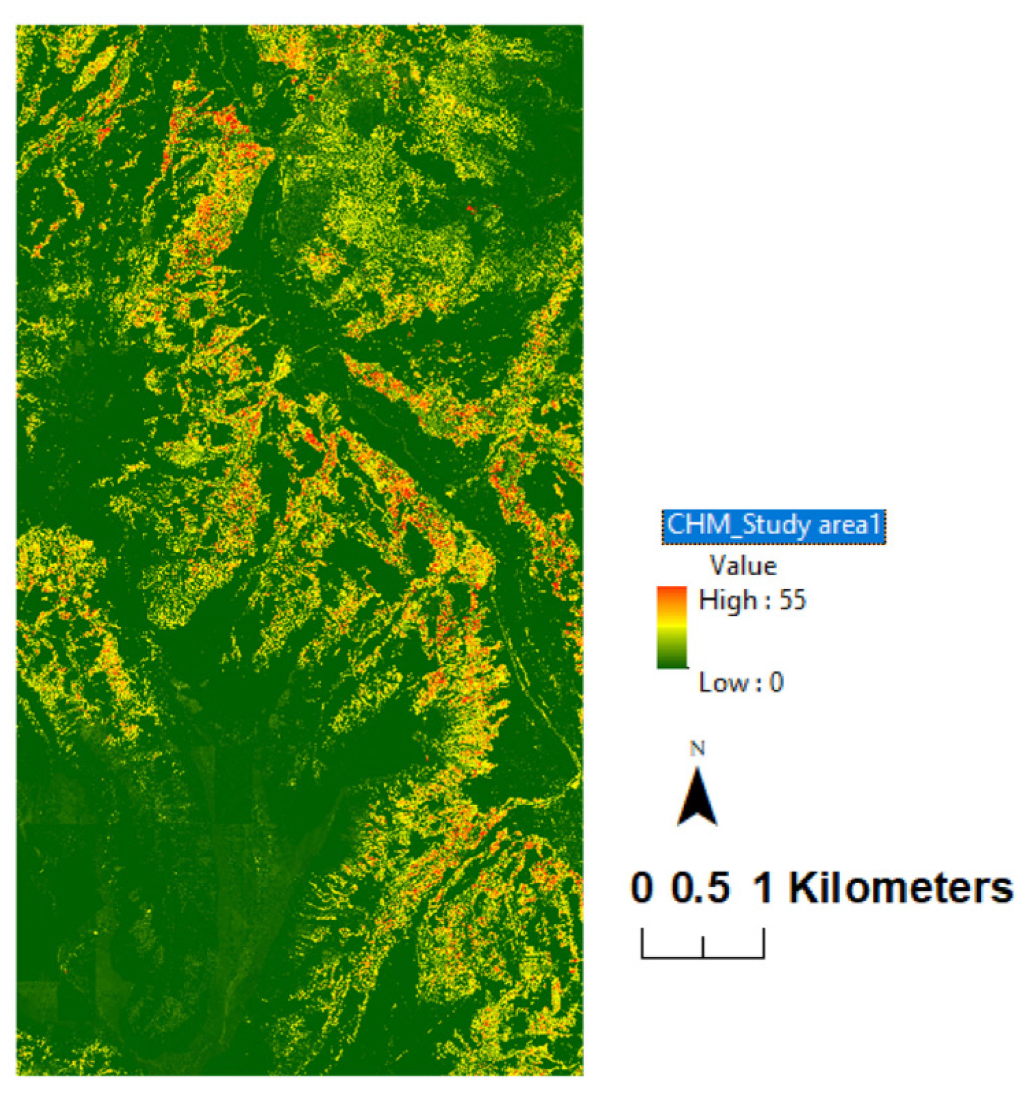
Airborne Laser Scanning (ALS) data, acquired in 16 June 2013, were used for study area 1 since it was closest to the acquisition of the aerial images. The ALS data were collected partly leaf-on/leaf-off with a point density of 20 points per m². From this data set, a normalized Digital Surface Model (nDSM) was generated. Buildings were removed using the building footprints Topographic Landscape Model (TLM) from swisstopo. This made it possible to generate a Canopy Height Model (CHM) (Figure 3).

2.3. Data Processing

2.3.1. Image Patches

Prior to setting up the CNN models, a regular grid of 50 m mesh size was generated for both study areas (Figure 4). From these grids, patches of 200 × 200 pixels were extracted from the B&W aerial images (spatial resolution of 0.25 m) from both time points. This was considered beneficial because the image patches were then equally sized, and no resizing operation was needed for the CNN model input. These patches did not overlap and could be considered spatially independent images that included all in-class and between-class variability of the three target classes “dense forest”, “group of trees”, and “other”. Moreover, the distinction between these three classes per image patch was facilitated by calculation of the vegetation cover proportional ratio (more detail can be found in Section 2.3.2) using the Vegetation Height Model (VHM) generated from ALS point cloud data.

2.3.2. Forest Structure Classes

Forest structure classes were determined based on ALS data. The three structure classes “dense forest”, “group of trees”, and “other” were defined based on percentage of Canopy Cover (CC) values and two different height classes. For this step, two classes of height and several classes of percentage of CC were calculated per grid cell (see

Table 1. Definitions of the three vegetation structure classes “dense forest”, “group of trees”, and “other” based on Canopy Cover (CC) percentage and height, as extracted per 50 × 50 m image patch.

Structure Class	Description
Dense forest	>20% CC height value of pixels >5 m
Group of trees	2–20% CC height value of pixels >5 m and <5% CC height value of pixels 3–5 m
Other	(1) <2% CC height value of pixels >5 m and >5% CC height value of pixels 3–5 m (2) <1% CC height value of pixels 3–5 m

).

The selection of the two height classes was based on the focus on changes in treeline ecotones. Vegetation smaller than 3 m in height was excluded. The first class includes CC percentages for all pixels greater than 5 m height and the second class includes the CC percentage for all pixels in the height range of 3–5 m. Figure 5a–c shows the two height classes of percentages of CC for study area 1.

2.3.3. Data Labelling

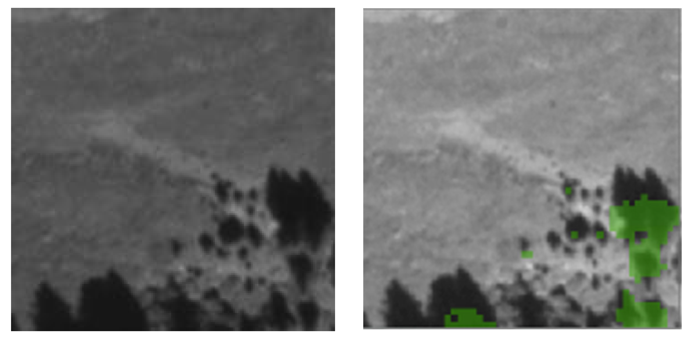
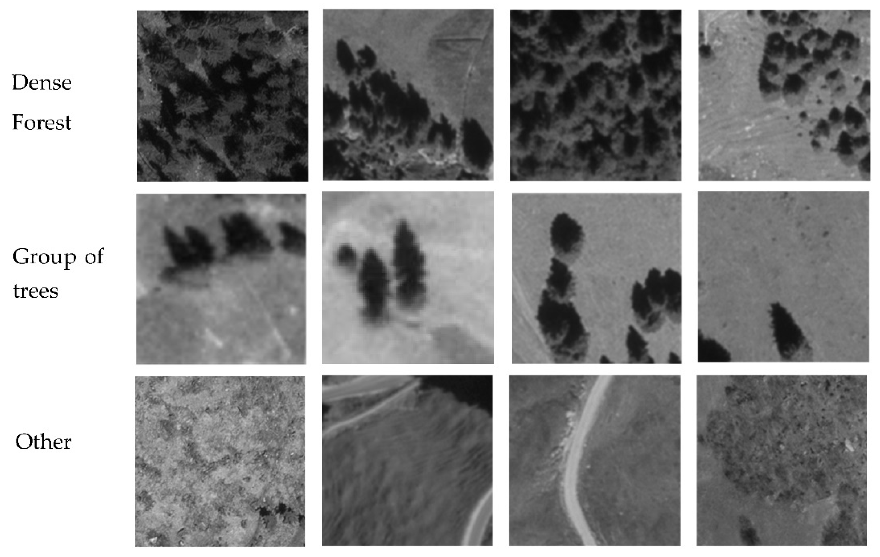
Based on the definitions described in Table 1, the 50 × 50 m image patches from Img_T2 for both study areas were extracted separately and labeled with the corresponding class. These labeled image patches were then taken as the first candidate sets for each class. Then, an active interaction was manually added to remove irrelevant data. Figure 6 shows an example of how cleaning was applied to the training data set of the first candidates, where the green color indicates the pixels with h > 5 m. This was a candidate for the class “dense forest” based on the definition in Table 1, but it can be predicted by CNNs model as the “group of trees” class. Figure 7 shows examples of image patches of the three classes that were used as training data.

2.4. Training and Validation Data

2.4.1. Training Data

In contrast to time point 2 (images from 2009 and 2010), no corresponding CHMs were available for time point 1 (images from 1980) in the present study. Thus, the initial idea was to use the images from time point 2 that were labeled using CHMs for model training to predict images from Img_T1 (1980). Usually, more precise predictions are achieved if the training data are representative of the underlying distributions. However, there were large differences between Img_T1 and Img_T2 for both study areas because of different image acquisition conditions and techniques. In order to improve the adaption of the CNN model for the historical aerial images, an interactive approach was set up to generate the training data. Image patches (Img_T1) with incorrect predictions from the initial trained model were actively added and extracted into the training data set and the model was re-run. This procedure consisted of four main steps:

• Generation of the first training (80%) and validation (20%) data set using Img_T2 from study area 1. The data labeling was conducted based on the CHM obtained from ALS data and the CC percentage of each image patch;
• Model training and prediction based on the first available data set for Img_T1 of study area 1 and for Img_T1 and Img_T2 of study area 2;
• Interactive addition of all image patches (80% for training, 20% for validation) that were wrongly predicted into the model to increase the model’s generalization;
• Re-running of the model training. At the end, for the first-level training data set (CNN1), there were 11,932 image patches from Img_T2 in study area 1, 227 image patches from Img_T1 in study area 1, 330 image patches from Img_T1 in study area 2, and 60 image patches from Img_T2 in study area 2. Since sufficient training data for the class “group of trees” were not available, we added augmented image patches, e.g., the mirrored images with vertical and horizontal flips, to this class. After these steps, we used 6892 image patches for the class “dense forest”, 2519 image patches for “group of trees”, and 6509 image patches for “other”.

2.4.2. Independent Validation Data

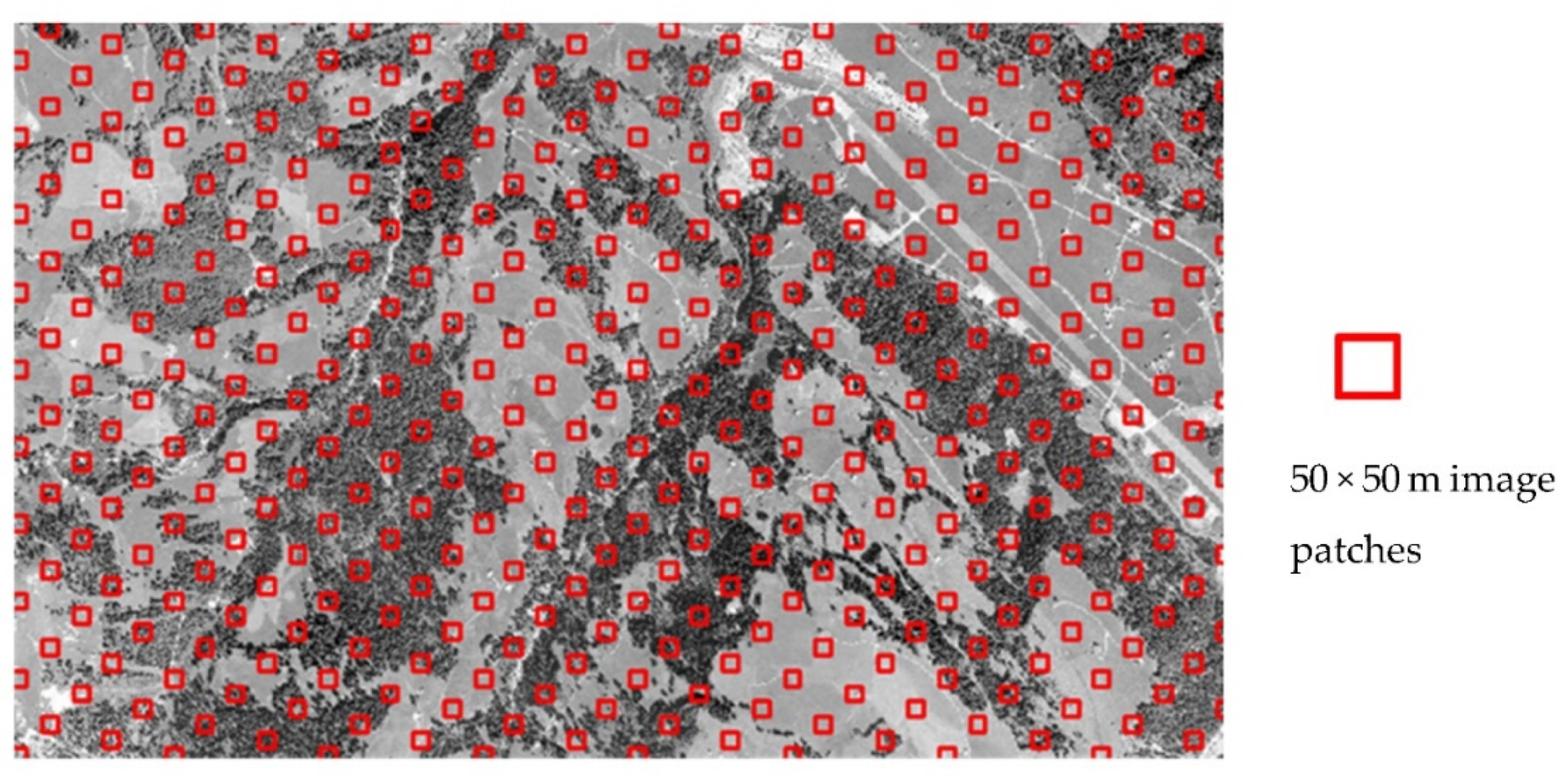
The predictions from the CNN models were evaluated using visual image interpretation of patches from both time points. For this, the interpretation of the image patches was carried out on an equal interval sampling grid (Figure 8) for the three classes “dense forest”, “group of trees”, and “other”. In total, 3845 image patches (10%) of study area 1 and 1581 image patches (20%) of study area 2 were interpreted in order to avoid exceeding heavy manual workload.

2.5. Methods

2.5.1. Overview of the Classification Approach

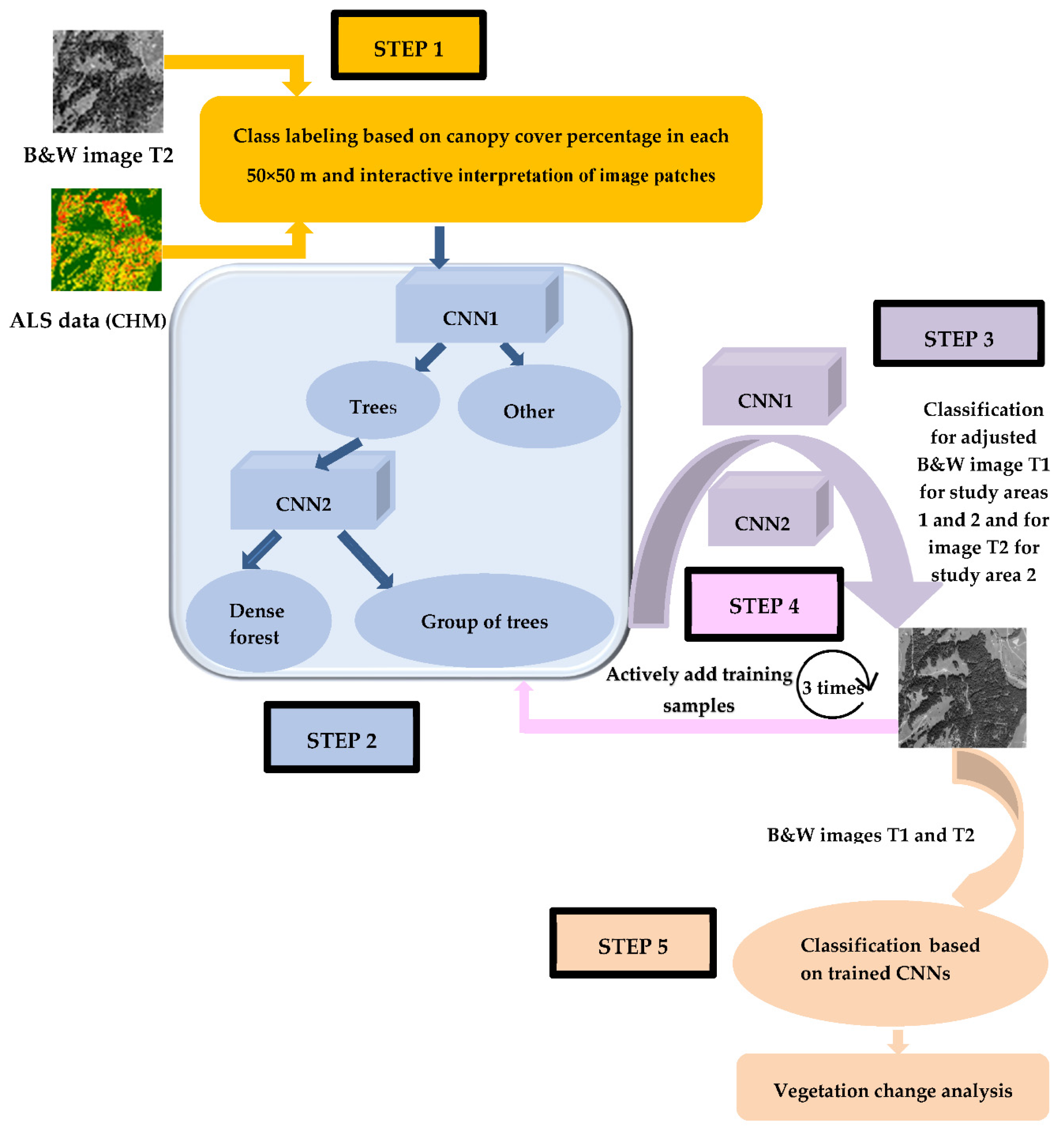
The workflow of the classification approach is given in Figure 9 and consisted of five main steps:

• Calculation of Canopy Cover (CC) percentage from CHMs obtained from the ALS point data from 2010 (Img_T1) in study area 1 and active interaction and labeling of each potential image patch (50 × 50 m);
• Training using a hierarchical Convolutional Neural Network (CNN) using the information on the labeled image patches;
• Classification of images from 1980 (Img_T1) from study area 1 and from 1980 (Img_T1) & 2009 (Img_T2) from study area 2 based on trained CNNs;
• Active addition of training samples from wrongly predicted image patches, e.g., predicted as class “other” instead of “group of trees”.
• Evaluation of the change in forest cover between the two time points.

2.5.2. AlexNet

In the present study, two CNNs were trained based on a pre-trained AlexNet CNN. The AlexNet is capable of solving the problem of general image classification for realistic objects over a large data set [35]. The network consists of eight layers: five convolutional layers (some of them are followed by max-pooling layers), two fully connected layers, and one fully connected output layer (Figure 10). Moreover, it involves a dropout technique with a dropout rate of 0.2 to prevent overfitting after each fully connected layer. An averaged stochastic gradient descent (ASGD) optimizer was selected because of its superb performance [36]. Each CNN was trained over 30 epochs using a batch size of 64 that was maintained across all networks. We used a learning rate of 0.01 in the optimization process, and we used Rectified Linear Unit (ReLU) as the activation function. Moreover, the cross-entropy cost function was applied as a loss function.

2.5.3. Hierarchical Classification Strategy

In this study, to distinguish between the three classes “dense forest”, “group of trees”, and “other”, two binary classification models were trained. First, a CNN (CNN1, see Figure 9) was trained to distinguish “vegetation” from other land cover, where “vegetation” was an aggregated class including “dense forest” and “group of trees”. Then, another CNN (CNN2, see Figure 9) was trained to separate the classes “dense forest” and “group of trees”. The final classification results were based on these two CNNs. The idea behind this hierarchical classification approach was that most of the traditional CNN-based classifications are so-called “flat classifiers” with an underlying assumption that all classes are equally difficult to distinguish [37]. Traditionally, the CNN network learns to extract relevant features and to classify such images. This trained model was then used to classify unlabeled image patches. In these training steps, all the training data are represented in the network during the same training process. However, visual separability between different object categories is highly uneven in the real world, which means that we rarely have all the information at once. Important information may become lost if the natural hierarchy of the data is ignored. Since we had to deal with shared characteristics among the classes, we first merged them based on these characteristics and exploited their relationships (step 2 in Figure 9).

2.5.4. Adjusting Historical Images

In the present study, greyscale images from 2010 were used to train the models and then the prediction was implemented to the historical B&W images from 1980. Differences between the images from two time points include image resolution, contrast, illumination, and texture. These differences may result in the wrong prediction because of the unlike distribution of training and test data. In order to minimize the bias affected by the different conditions between the training and testing stages, intensity values for the historical B&W images were first adjusted (see Equation (1)). If I is the image and f(x,y) indicates the gray value of I at position (x,y), then the adjusted gray value can be calculated as follows:

$$f{\left(x,y\right)}_{adjust}=(f\left(x,y-\min \left(I\right)\right)/\left(\max \left(I\right)-\min \left(I\right)\right)$$

(1)

2.5.5. Disagreement Analysis

As the occurrence of trees depends on several factors, e.g., directly by soil, topography, and climate and indirectly by elevation, a disagreement analysis was carried out that was based on elevation classes. Prior to this, a normalization using 200 m steps (e.g., elevation category 800–1000 m a.s.l.) was applied over the elevation range of 800–3000 m a.s.l.

For the ith elevation category, we let N_t,i be the total number of image patches, N_{CNN-denseforest,i} the number of the image patches predicted as the class “dense forest” by the CNN, and N_{CNN-interpretation-denseforest,i} the number of image patches confirmed as the class “dense forest” by the CNN and visual image interpretation. We used the following definitions:

$$R_{CNN-denseforest,i}=N_{CNN-denseforest,i}/N_{t,i}$$

(2)

$$R_{CNN-interpretation-denseforest,i}=N_{CNN-interpretation-denseforest,i}/N_{t,i}$$

(3)

Then, with $\mathsf{\Psi }={\displaystyle \sum }_i{R}_{CNN-denseforest,i}$, the normalized ratio can be calculated as follows:

$${\rho }_{CNN-denseforest,i}=R_{CNN-denseforest,i}/\mathsf{\Psi }$$

(4)

$${\rho }_{CNN-interpretation-denseforest,i}=R_{CNN-interpretation-denseforest,i}/\mathsf{\Psi }$$

(5)

Therefore, the disagreement between the CNNs and visual image interpretation can be calculated as follows:

$$D_{CNN-denseforest-users,i}={\rho }_{CNN-denseforest,i}-{\rho }_{CNN-interpretation-denseforest,i}$$

(6)

$D_{CNN-denseforest-users,i}$ reflects the agreed difference between the number predicted by the CNN and the agreed number from both the CNNs and visual image interpretation based on the size of the elevation category. This measured difference is $D_{CNN-denseforest-users,i}$ and is similar to the user’s accuracy. By the same procedure, $D_{interpretation-denseforest-producers,i}$ reflects the agreed difference between visual image interpretation and the agreed number of the CNN and visual interpretation. This measured difference is $D_{interpretation-denseforest-producers,i}$ and is similar to the producer’s accuracy.

3. Results

3.1. Classifications

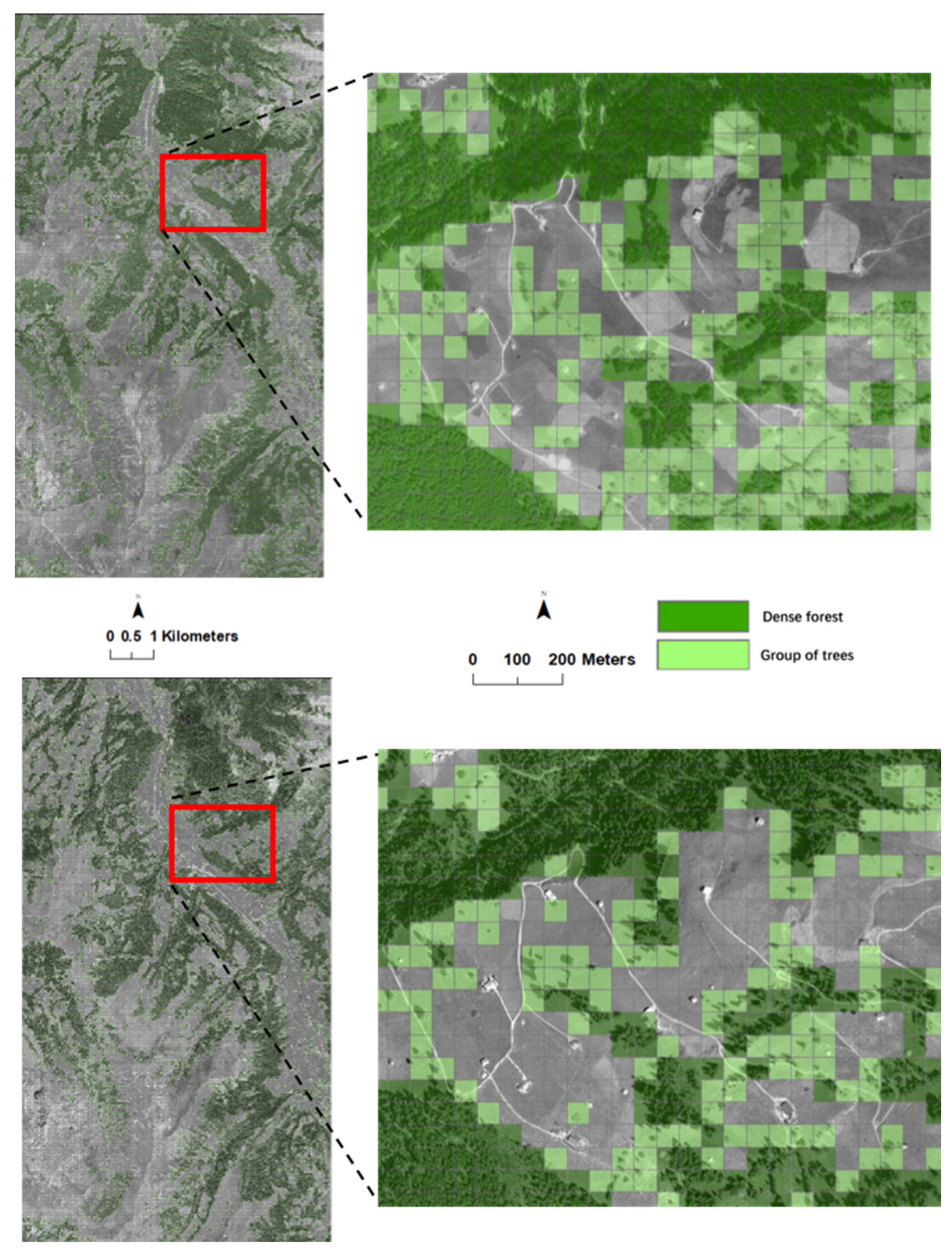
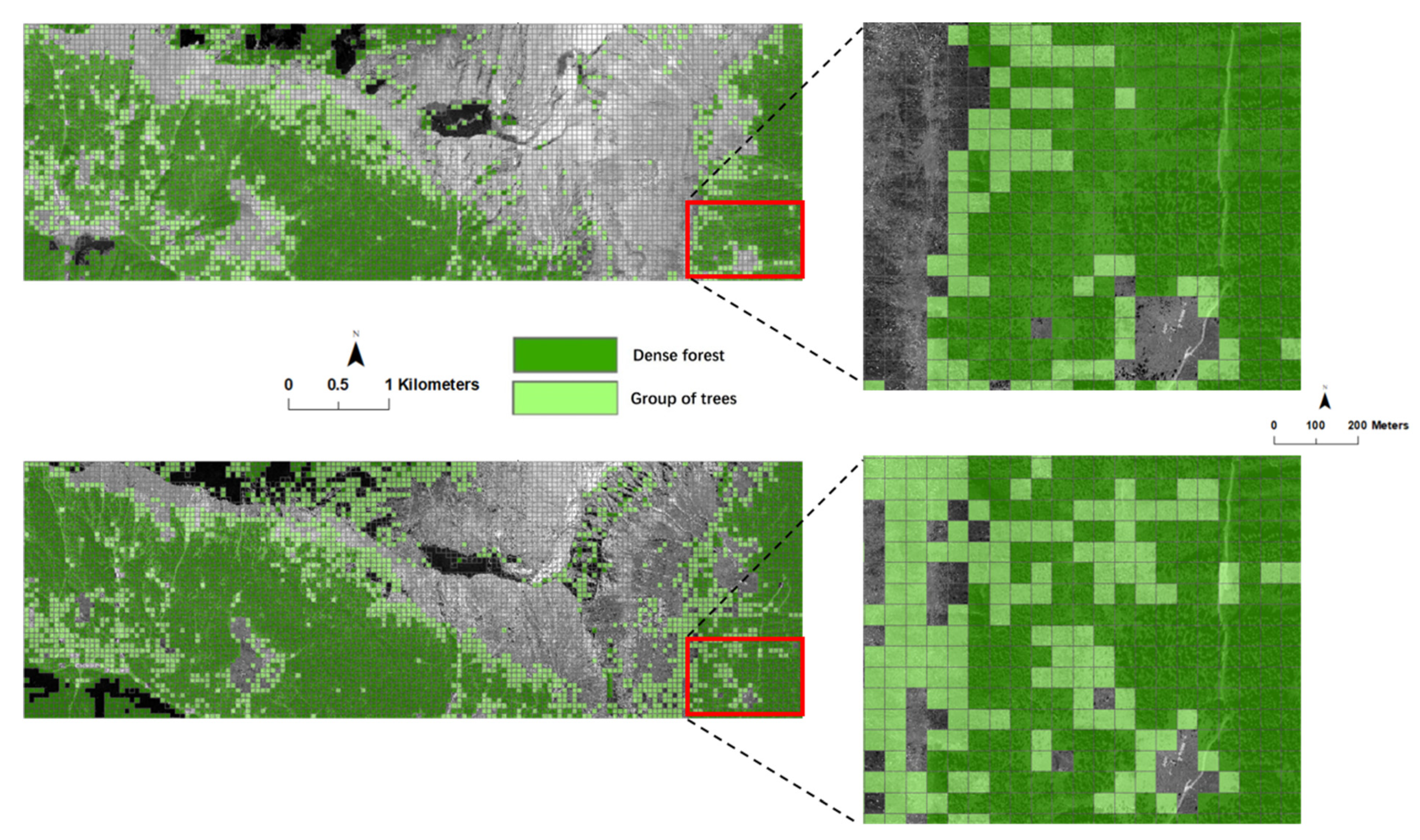
The maps of the three classes “dense forest”, “groups of trees”, and “other” for both study areas are shown in Figure 11 (study area 1) and Figure 12 (study area 2).

Figure 11 clearly shows that in study area 1 the class “dense forest” has increased overall, although selective forest management has been carried out within the 30 years. In contrast, the class “groups of trees” has decreased, in particular along the upper treeline. This decrease in shrub and trees is most probably due to an increase in the cultivation of pastures and meadows.

Figure 12 illustrates that the class “dense forest” has increased in some parts of study area 2. Moreover, the class “groups of trees” has increased in some parts, in particular along the upper treeline. This is typical for regions in the Southern Alps, in which only very selective forest management is carried out, which, together with less cultivated pastures, enables shrub encroachment.

Table 2. Agreement between classification and visual image interpretation for the three classes “dense forest”, “group of trees”, and “other”. Note that in study area 1 image patches from 2009 were used as training data and were therefore excluded from the agreement analysis.

Class	Agreement	Study Area 1	Study Area 2
		Img_T1 (1980)	Img_T1 (1980)	Img_T2 (2009)
Dense forest	User’s agreement	0.94	0.83	0.97
	Producer’s agreement	0.89	0.95	0.88
Group of trees	User’s agreement	0.67	0.47	0.51
	Producer’s agreement	0.60	0.27	0.30
Other	User’s agreement	0.83	0.83	0.76
	Producer’s agreement	0.94	0.84	0.95
	Overall agreement	0.85	0.80	0.84

shows the agreement for the three classes “dense forest”, “group of trees”, and “other” between the model predictions and visual image interpretations for the two study areas. For the agreement, all the training image patches were excluded. For study area 1, most of the training patches were taken from Img_T2 (2010), and so no agreement assessment was carried out. The lowest overall agreement (0.80) was achieved when image patches from 1980 were used for study area 2. A similar overall agreement was obtained in study area 1, with 0.85 for image patches from 1980, and in study area 2, with 0.84 for image patches from 2009.

The highest agreement (0.97) (user’s agreement) was obtained for the class “dense forest” in study area 2 using image patches from 2009. In contrast, the lowest (producer’s) agreement (0.27) was obtained for the class “group of trees” in study area 2 using image patches from 1980. In general, higher agreement was obtained for the classes “dense forest” and “other” than for “group of trees”.

Table 3. Overall user’s and producer’s agreement between classifications either with or without hierarchy and visual image interpretation for the three classes “dense forest”, “group of trees”, and “other”. Note that in study area 1 image patches from 2009 were used as training data and were therefore excluded from the agreement analysis.

Class	Agreement	Study Area 1 Img_T1 (1980)
		Hierarchical CNN	Non-Hierarchical CNN
Dense forest	User’s agreement	0.94	0.83
	Producer’s agreement	0.89	0.88
Group of trees	User’s agreement	0.67	0.67
	Producer’s agreement	0.60	0.53
Other	User’s agreement	0.83	0.78
	Producer’s agreement	0.94	0.83
	Overall agreement	0.85	0.79

shows the agreement in study area 1 based on image patches from 1980 when only a single CNN model was used (non-hierarchical) and when both CNN1 and CNN2 (hierarchical) were used. Both were directly trained with the three classes and using the same training data for each class. The comparison indicates that higher agreement can be achieved when the hierarchical classification is used.

3.2. Disagreement Analysis

Figure 13 shows the disagreement graphs for the class “dense forest” for each elevation category. The results are clustered based on the two time points, i.e., 1980 and 2009, for study area 2. The normalized variable D (measured differences) and variable $\mathsf{\rho }$ are stacked into one bar. Based on the definition of disagreement (see Section 2.5.5), the smaller the height of variable D compared with the normalized variable $\mathsf{\rho } \left(\mathrm{normalized} \mathrm{ratio}\right)$, the higher the agreement between predictions based solely on CNNs and visual image interpretation.

In Figure 13, a shorter length for variables D_{CNN-denseforest-users} and D_{interpretation-denseforest-producer} shows a better match between the classification and visual image interpretation for the elevation ranges between 1200 and 2000 m a.s.l. It also shows that some image patches were not classified as “dense forest” (indicated with the circle) compared with visual image interpretation, especially for Img_T1 (1980) in the elevation ranges between 800 and 1200 m a.s.l. The relatively longer length of variable D in both time points indicates a generally higher disagreement for higher elevation categories. The reason for this might be the relatively small number of image patches of the class “dense forest” that were visually interpreted.

3.3. Vegetation Change Depending on Elevation

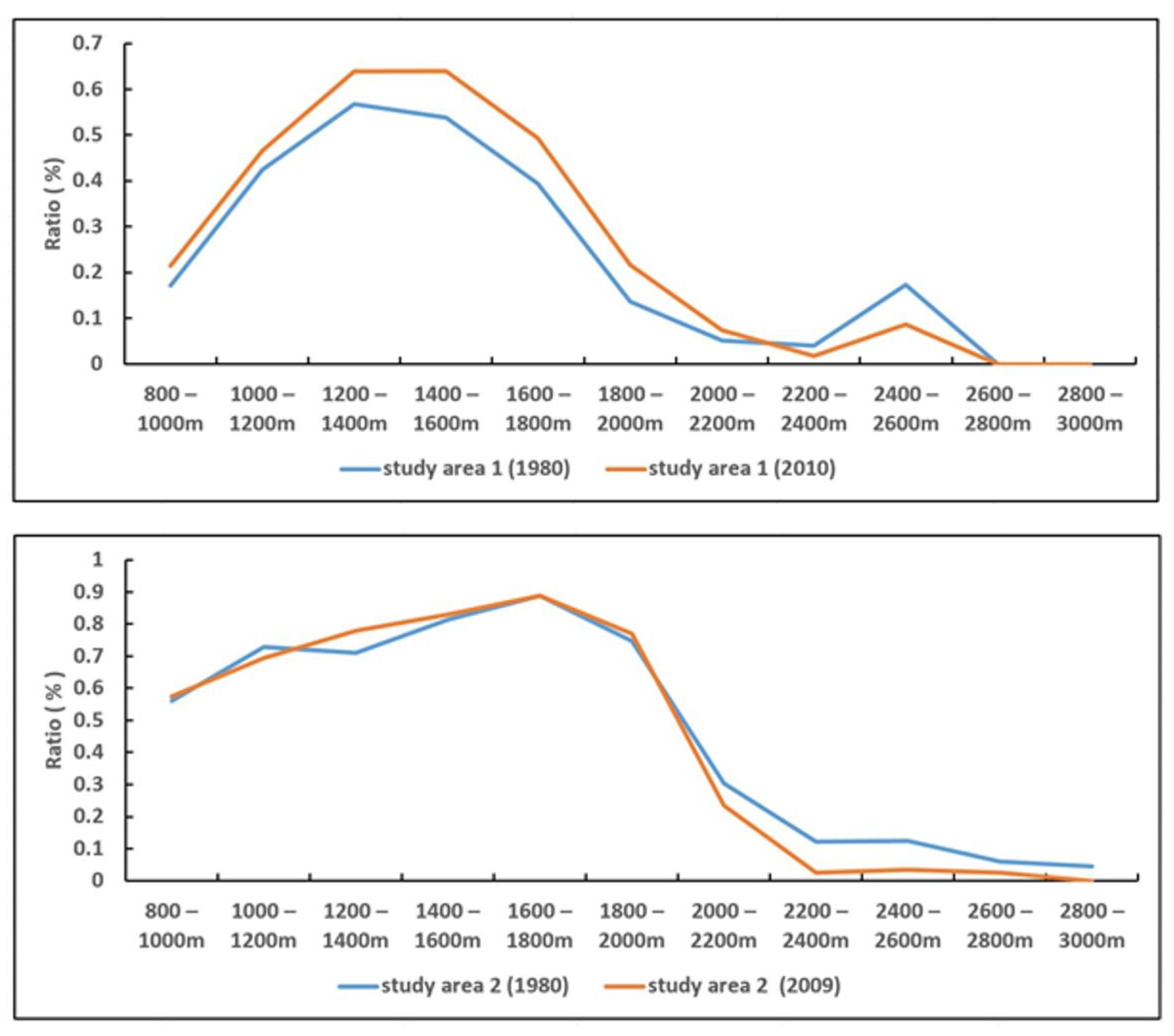
Figure 14 illustrates the distribution of the predicted image patches of the class “dense forest” along the normalized elevation categories for the two time points in the two study areas. The different changes suggest different pattern changes in the class “dense forest” between study areas 1 and 2. While for study area 1 there was a general increase in the “dense forest” class in most elevation categories, for study area 2, a decrease in the “dense forest” class was found in higher elevation categories. The distributions are relatively similar for the two time points for elevations lower than 2000 m a.s.l.

4. Discussion

4.1. General Aspects of the Proposed Method

The present study confirms the suitability of CNNs in combination with B&W aerial images for assessing changes over 30 years in alpine upper treeline ecotones using the three vegetation structure classes “dense forest”, “group of trees”, and “other”. A comparison with visual image interpretation revealed general high agreement for the class “dense forest” and lower agreement for the class “group of trees”.

The use of CHMs based on ALS data substantially reduced the workload for the selection of appropriate training data. In particular, interactive addition of wrongly predicted image patches from time point T1 (1980) resulted in overall improvements to the models, and the adapted models were beneficial for images of time point T1. The use of radiometrically adjusted images as the input for model prediction substantially minimized data shift problems between the two time points.

The two main advantages of the interactive steps are: (1) little manual work was needed for the selection of training data since the focus was placed on incorrectly predicted image patches only; (2) adding image patches from time point 1 (1980) increased the correct classification rates of the models.

A reliable interpretation of the classification comparison was possible by analyzing per class disagreement between the classification models and visual image interpretation of 5426 image patches. Nevertheless, the lowest agreement was obtained for the class “group of trees”, and the use of this class is only partly satisfactory. In comparison to other commonly used CNN approaches for land cover classifications on recent remote sensing data, our approach using historical aerial images was less effective. The key task of CNNs, to obtain representative features from image objects during training, was limited to a certain degree since historical images only provided a single band.

The use of single-band B&W images was challenging for images from all dates (1980 and 2009, 2010) and occurred during model training and prediction. The main reason was the heterogeneity of the image patches (between Img_T1 and Img_T2) regarding image quality and properties, i.e., spectral distortion, brightness, and contrast.

4.2. Performance Differences between “Dense Forest” and “Group of Trees”

In this section, the disagreement between the CNNs and visual image interpretation is discussed. A potential source of disagreement is related to the image distortion of historical B&W images (Img_T1).

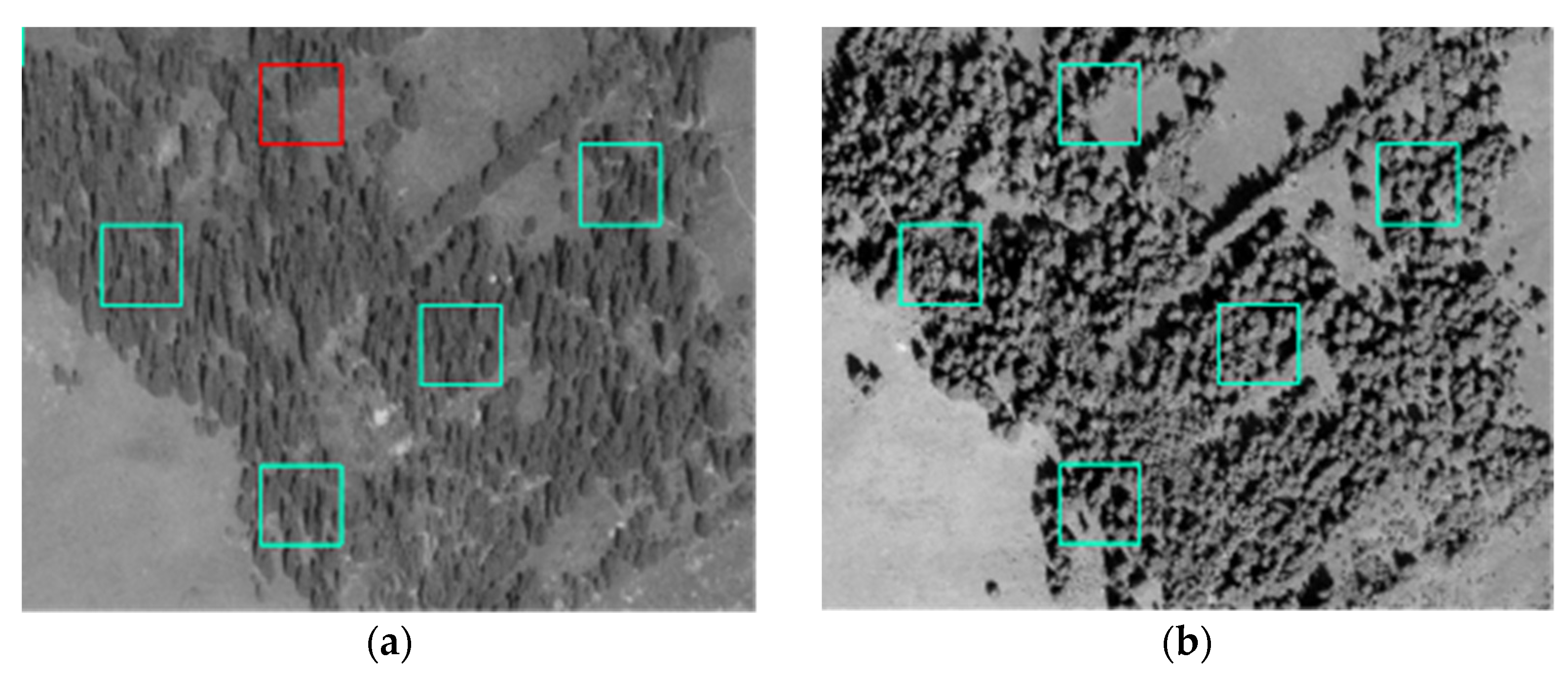
Figure 15a illustrates this disagreement and shows the different qualities of the B&W images. The blue-green boxes show image patches that were both correctly classified as “dense forest” and confirmed by visual image interpretation. In contrast, the red box shows an image patch from 1980 (Img_T1) with disagreement for the two classes “dense forest” (obtained by visual image interpretation) and “group of trees” (obtained by the CNN models). Figure 15b illustrates agreement for the class “dense forest” obtained by the CNN classification and visual image interpretation when using images from 2009 (Img_T2). Figure 15 indicates that although CNNs have a certain degree of generalization ability, they are not able to achieve satisfactory classification results on different source images in the case of large differences in acquisition conditions.

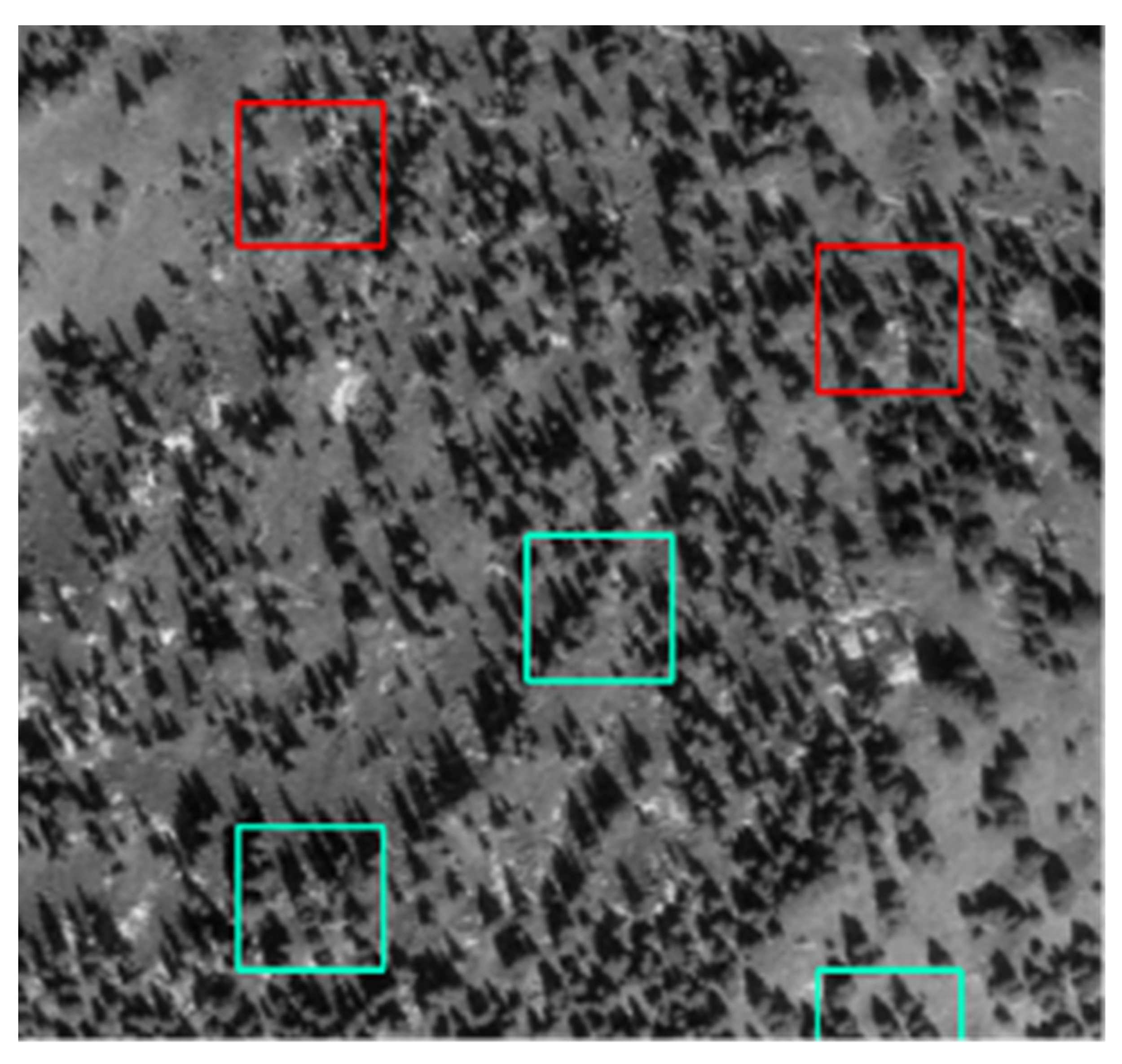
Another potential source of disagreement is related to the unclear boundary for the semantic concept definition of the three classes. Class definition might be used differently in CNNs and in visual image interpretation. Figure 16 shows an image patch (from Img_T1) with disagreement between the two classes “group of trees” (obtained by CNNs) and “dense forest” (obtained by visual image interpretation).

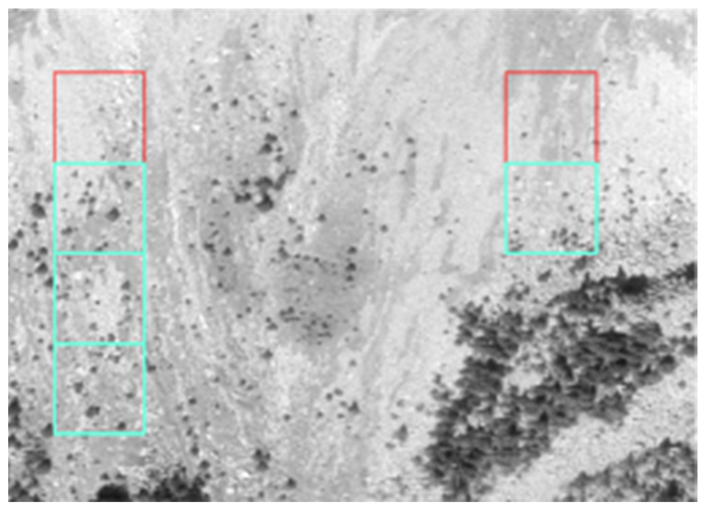
Moreover, disagreement between CNN and visual image interpretation also occurred for image patches that contained very small trees where the same tree was not always recognized by the CNNs. Figure 17 illustrates that CNNs classified some image patches as “other”, while they were assigned to “group of trees” by visual image interpretation.

The present study reveals that, overall, disagreement between CNNs and visual image interpretation was more pronounced for study area 2 than for study area 1. This might also be related to the fact that study area 1 is in the southern Swiss Alps and is characterized by a higher variability of forest structure and very little forest management. As a direct consequence of the disagreement, relatively poor user’s agreement was obtained as well, e.g., 32% user’s agreement for images acquired in 2009. In our study, we assume that visual image interpretation was more robust due to the extensive experience of the interpreters. Thus, the smaller the difference between classes, the more pronounced the divergence between human and CNN classification.

A couple of studies [38,39] have indicated that CNN models tend to exhibit lower performance when the object in the scene is far away. Therefore, we emphasize that the difference between our classification models and visual image interpretation is a disagreement rather than an absolute classification error.

4.3. Impacts on Classification

Factors that impacted classification can be summarized as follows:

The first factor is related to image quality, such as lighting, distortion, scale, and blur, which had a direct impact on the classification and was partly solved by adjusting images accordingly. The second factor is related to the differences between the three classes “dense forest”, “group of trees”, and “other”, which were relatively large and were the reason for a higher user’s and producer’s agreement for the class “other”. The third factor is related to the problem of the initial fine-grained classifications and the differences between visual image interpretation and classification algorithms. Thus, a class might be differently interpreted and defined by humans than by CNNs, which use abstract definitions based on functions. This makes it more difficult for classification models to understand the classified objects.

In the present study, definitions of the three classes were formed using the structure information from the ALS point cloud data with several predefined thresholds. To a certain degree, this might be the reason for blurred class differences and disagreements (Figure 16). As [40] pointed out, human visual object recognition is typically and largely independent of the viewpoint and object orientation. They concluded that marked differences in the way humans and current CNNs perform visual object recognition may still remain.

4.4. Forest Cover Change Per Elevation Category

While in study area 1, the changes between 1980 and 2010 mainly occurred in parts within large forest areas, always below the upper treeline, in study area 2, the changes additionally occurred near the treeline ecotones. The class “dense forest” generally increased in most elevation categories in study area 1. In contrast, the same was only found in higher elevation categories in study area 2. Moreover, the forest structure in the treeline ecotones of study area 2 seems to have become more diverse, in particular in the transition zones between shrubs, single trees, and dense forest.

There are several possible reasons for these differences. First, they might be related to the different biogeographical regions (Figure 1) of the two study areas, with different climatic conditions and vegetation composition having a direct impact on forest structure. Tree species composition of the two study areas also differs. While in both study areas the proportion of coniferous tree species increases with increasing elevation, broadleaved tree species are more dominant in study area 1, which has generally lower elevations. Together with active forest management in study area 1 and little forest management in study area 2, this might be the main driver for the establishment of different conditions in these treeline ecotones. Thus, different patterns of forest change can be observed for the two study areas, depending on the elevation category (Figure 14).

4.5. Future Work

Historical B&W aerial images serve as a valuable source of information for studying past land cover and land use and their change to a certain degree. However, as their quality is limited and the information is provided in a single band, their use in classifying natural objects such as trees and forests remains challenging. Thus, future research should also include texture information [41,42]. Texture information from images is an important characteristic, as it is a function of spatial variation in pixel intensity [43]. Additional information about the structural arrangement of objects and their relationship with respect to their local neighborhoods will be beneficial and increase the inter-class distance between “dense forest” and “group of trees”.

It is well recognized that a large data set of high-quality training data is needed for machine learning and DL approaches. In our study, we experienced a probable conceptual gap between the interpreter and the classification models. Human visual perception is much more robust than that of CNN models because human visual perception is not simply function mapping but has evolved over a long period and incorporates various factors, such as target detection, background filtering, association, decision making, and reasoning, intertwined in a very fine intelligent system [44]. Thus, migrating cognitive power to CNNs remains challenging. Therefore, a promising approach would be to include findings from Deng et al. [45] on integrating the model with human knowledge. For example, [46] successfully implemented a human cognitive model to reduce the gap between human beings and machines in this type of inference by utilizing cognitive biases. The proposed method is promising and will be applied to larger areas. Thus, changes in treeline ecotones could be assessed for entire countries and help to reconstruct and better understand forest changes over the last decades at a high spatial resolution.

5. Conclusions

Historical B&W aerial images are a valuable source of information to unveil landscapes in the past and reconstruct changes up to the present. In this paper, we demonstrate that changes over 30 years in woody vegetation cover along Alpine treeline ecotones can be assessed for two different biogeographic study areas with different managements in the Swiss mountains. A CNN-based classification approach was set up for the three categories “dense forest”, “group of trees”, and “others”, using recent ALS data for the selection of appropriate training data. The study shows the benefits of actively trained CNNs using hierarchical strategies. While generally encouraging results were obtained, visual image interpretation revealed high agreement for “dense forest” and lower agreement for “group of trees”. Sources of disagreements were related to image distortion and problems with short trees. With the proposed method, the assessment of high-resolution, long-term vegetation dynamics at tree line ecotones became feasible and is very promising for area-wide applications. The additional use of texture information in future studies might further increase the inter-class distance between “dense forest” and “group of trees”.

References

1. Song, X.-P.; Hansen, M.C.; Stehman, S.V.; Potapov, P.V.; Tyukavina, A.; Vermote, E.F.; Townshend, J.R. Global land change from 1982 to 2016. Nature 2018, 560, 639–643. [Google Scholar] [CrossRef] [PubMed]
2. Chapin, F.S., III; Mcguire, A.D.; Randerson, J.; Pielke, R.; Baldocchi, D.; Hobbie, S.E.; Roulet, N.; Eugster, W.; Kasischke, E.; Rastetter, E.B.; et al. Arctic and boreal ecosystems of western North America as components of the climate system. Glob. Change Biol. 2000, 6, 211–223. [Google Scholar] [CrossRef] [PubMed] [Green Version]
3. Körner, C.; Paris, C.; Banzet, P. Alpine Plant Life: Functional Plant Ecology of High Mountain Ecosystems; With 47 Tables; Springer: Berlin/Heidelberg, Germany, 2003. [Google Scholar]
4. Colwell, R.K.; Brehm, G.; Cardelús, C.L.; Gilman, A.C.; Longino, J.T. Global warming, elevational range shifts, and lowland biotic attrition in the wet tropics. Science 2008, 322, 258–261. [Google Scholar] [CrossRef] [PubMed] [Green Version]
5. Løkken, J.O.; Evju, M.; Söderström, L.; Hofgaard, A. Vegetation response to climate warming across the forest tundra ecotone: Species dependent upward movement. J. Veg. Sci. 2020, 31, 854–866. [Google Scholar] [CrossRef]
6. Bolton, D.K.; Coops, N.C.; Hermosilla, T.; Wulder, M.A.; White, J.C. Evidence of vegetation greening at alpine treeline ecotones: Three decades of Landsat spectral trends informed by lidar-derived vertical structure. Environ. Res. Lett. 2018, 13, 10. [Google Scholar] [CrossRef]
7. Dirnbäck, T.; Essl, F.; Rabitsch, W. Disproportional risk for habitat loss of high-altitude endemic species under climate change. Glob. Change Biol. 2011, 17, 990–996. [Google Scholar] [CrossRef]
8. Morley, P.J.; Donoghue, D.N.M.; Chen, J.-C.; Jump, A.S. Quantifying structural diversity to better estimate change at mountain forest margins. Remote Sens. Environ. 2019, 223, 291–306. [Google Scholar] [CrossRef]
9. Bader, M.Y.; Llambí, L.D.; Case, B.S.; Buckley, H.L.; Toivonen, J.M.; Camarero, J.J.; Cairns, D.M.; Brown, C.D.; Wiegand, T.; Resler, L.M. A global framework for linking alpine-treeline ecotone patterns to underlying processes. Ecography 2021, 44, 265–292. [Google Scholar] [CrossRef]
10. Manzanedo, R.D.; Pederson, N. Towards a more ecological dendroecology. Tree-Ring Res. 2019, 75, 152–159, 158. [Google Scholar] [CrossRef]
11. Virtanen, R.; Luoto, M.; Rämä, T.; Mikkola, K.; Hjort, J.; Grytnes, J.-A.; Birks, H.J.B. Recent vegetation changes at the high-latitude tree line ecotone are controlled by geomorphological disturbance, productivity and diversity. Glob. Ecol. Biogeogr. 2010, 19, 810–821. [Google Scholar] [CrossRef]
12. Cserhalmi, D.; Nagy, J.; Kristóf, D.; Neidert, D. Changes in a wetland ecosystem: A vegetation reconstruction study based on historical panchromatic aerial photographs and succession patterns. Folia Geobot. 2011, 46, 351–371. [Google Scholar] [CrossRef]
13. Waser, L.T.; Boesch, R.; Wang, Z.; Ginzler, C. Towards Automated Forest Mapping; Springer: New York, NY, USA, 2017. [Google Scholar]
14. Pasetto, D.; Arenas-Castro, S.; Bustamante, J.; Casagrandi, R.; Chrysoulakis, N.; Cord, A.F.; Dittrich, A.; Domingo-Marimon, C.; El Serafy, G.; Karnieli, A.; et al. Integration of satellite remote sensing data in ecosystem modelling at local scales: Practices and trends. Methods Ecol. Evol. 2018, 9, 1810–1821. [Google Scholar] [CrossRef] [Green Version]
15. Afaq, Y.; Manocha, A. Analysis on change detection techniques for remote sensing applications: A review. Ecol. Inform. 2021, 63, 101310. [Google Scholar] [CrossRef]
16. Resler, L.M.; Fonstad, M.A.; Butler, D.R. Mapping the alpine Tteeline ecotone with digital aerial photography and textural analysis. Geocarto Int. 2004, 19, 37–44. [Google Scholar] [CrossRef]
17. Hill, R.A.; Granica, K.; Smith, G.M.; Schardt, M. Representation of an alpine treeline ecotone in SPOT 5 HRG data. Remote Sens. Environ. 2007, 110, 458–467. [Google Scholar] [CrossRef]
18. Næsset, E.; Nelson, R.F. Using airborne laser scanning to monitor tree migration in the boreal-alpine transition zone. Remote Sens. Environ. 2007, 110, 357–369. [Google Scholar] [CrossRef]
19. Carlson, B.Z.; Corona, M.C.; Dentant, C.; Bonet, R.; Thuiller, W.; Choler, P. Observed long-term greening of alpine vegetation—A case study in the French Alps. Environ. Res. Lett. 2017, 12, 114006. [Google Scholar] [CrossRef]
20. Mohapatra, J.; Singh, C.P.; Tripathi, O.P.; Pandya, H.A. Remote sensing of alpine treeline ecotone dynamics and phenology in Arunachal Pradesh Himalaya. Int. J. Remote Sens. 2019, 40, 7986–8009. [Google Scholar] [CrossRef]
21. He, W.; Ye, C.; Sun, J.; Xiong, J.; Wang, J.; Zhou, T. Dynamics and drivers of the alpine timberline on Gongga mountain of Tibetan Plateau-adopted from the Otsu method on google earth engine. Remote Sens. 2020, 12, 2651. [Google Scholar] [CrossRef]
22. Kadmon, R.; Harari-Kremer, R. Studying long-term vegetation dynamics using digital processing of historical aerial photographs. Remote Sens. Environ. 1999, 68, 164–176. [Google Scholar] [CrossRef]
23. Altuntas, C. Urban area change dection using time series aerial images. Int. Arch. Photogramm. Remote Sens. Spat. Inf. Sci. 2018, XLII-2, 29–34. [Google Scholar] [CrossRef] [Green Version]
24. Fox, A.J.; Cooper, A.P.R. Climate-change indicators from archival aerial photography of the Antarctic Peninsula. Ann. Glaciol. 1998, 27, 636–642. [Google Scholar] [CrossRef] [Green Version]
25. Vargo, L.J.; Anderson, B.M.; Horgan, H.J.; Mackintosh, A.N.; Lorrey, A.M.; Thornton, M. Using structure from motion photogrammetry to measure past glacier changes from historic aerial photographs. J. Glaciol. 2017, 63, 1105–1118. [Google Scholar] [CrossRef] [Green Version]
26. Mast, J.N.; Veblen, T.T.; Hodgson, M.E. Tree invasion within a pine/grassland ecotone: An approach with historic aerial photography and GIS modeling. For. Ecol. Manag. 1997, 93, 181–194. [Google Scholar] [CrossRef]
27. Cunningham, M.A. Accuracy assessment of digitized and classified land cover data for wildlife habitat. Landsc. Urban Plan. 2006, 78, 217–228. [Google Scholar] [CrossRef]
28. Sylvain, J.-D.; Drolet, G.; Brown, N. Mapping dead forest cover using a deep convolutional neural network and digital aerial photography. ISPRS J. Photogramm. Remote Sens. 2019, 156, 14–26. [Google Scholar] [CrossRef]
29. Xi, Y.; Ren, C.; Wang, Z.; Wei, S.; Bai, J.; Zhang, B.; Xiang, H.; Chen, L. Mapping tree species composition using OHS-1 hyperspectral data and deep learning algorithms in Changbai mountains, Northeast China. Forests 2019, 10, 818. [Google Scholar] [CrossRef] [Green Version]
30. Fricker, G.A.; Ventura, J.D.; Wolf, J.A.; North, M.P.; Davis, F.W.; Franklin, J. A convolutional neural network classifier identifies tree species in mixed-conifer forest from hyperspectral imagery. Remote Sens. 2019, 11, 2326. [Google Scholar] [CrossRef] [Green Version]
31. Rehush, N.; Abegg, M.; Waser, L.T.; Brändli, U.-B. Identifying tree-related microhabitats in TLS point clouds using machine learning. Remote Sens. 2018, 10, 1735. [Google Scholar] [CrossRef] [Green Version]
32. Ball, J.E.; Anderson, D.T.; Chan, C.S. Comprehensive survey of deep learning in remote sensing: Theories, tools, and challenges for the community. J. Appl. Remote Sens. 2017, 11, 042609. [Google Scholar] [CrossRef] [Green Version]
33. Alam, M.; Wang, J.-F.; Guangpei, C.; Yunrong, L.V.; Chen, Y. Convolutional neural network for the semantic segmentation of remote sensing images. Mob. Netw. Appl. 2021, 26, 200–215. [Google Scholar] [CrossRef]
34. Kattenborn, T.; Leitloff, J.; Schiefer, F.; Hinz, S. Review on Convolutional Neural Networks (CNN) in vegetation remote sensing. ISPRS J. Photogramm. Remote Sens. 2021, 173, 24–49. [Google Scholar] [CrossRef]
35. Krizhevsky, A.; Sutskever, I.; Hinton, G.E. ImageNet classification with deep convolutional neural networks. Commun. ACM 2017, 60, 84–90. [Google Scholar] [CrossRef]
36. Sun, X.; Kashima, H.; Matsuzaki, T.; Ueda, N. Averaged stochastic gradient descent with feedback: An accurate, robust, and fast training method. In Proceedings of the 2010 IEEE International Conference on Data Mining, Sydney, Australia, 13–17 December 2010; pp. 1067–1072. [Google Scholar]
37. Fu, R.; Li, B.; Gao, Y.; Wang, P. CNN with coarse-to-fine layer for hierarchical classification. IET Comput. Vis. 2018, 12, 892–899. [Google Scholar] [CrossRef]
38. Miao, Z.; Gaynor, K.M.; Wang, J.; Liu, Z.; Muellerklein, O.; Norouzzadeh, M.S.; McInturff, A.; Bowie, R.C.K.; Nathan, R.; Yu, S.X.; et al. Insights and approaches using deep learning to classify wildlife. Sci. Rep. 2019, 9, 8137. [Google Scholar] [CrossRef]
39. Alganci, U.; Soydas, M.; Sertel, E. Comparative research on deep learning approaches for Airplane detection from very high-resolution satellite images. Remote Sens. 2020, 12, 458. [Google Scholar] [CrossRef] [Green Version]
40. Geirhos, R.; Janssen, D.H.; Schütt, H.H.; Rauber, J.; Bethge, M.; Wichmann, F.A. Comparing deep neural networks against humans: Object recognition when the signal gets weaker. arXiv 2017, arXiv:1706.06969. [Google Scholar]
41. Ji, M.; Liu, L.; Du, R.; Buchroithner, M.F. A Comparative study of texture and convolutional neural network features for detecting collapsed buildings after earthquakes using pre- and post-event satellite imagery. Remote Sens. 2019, 11, 1202. [Google Scholar] [CrossRef] [Green Version]
42. Davies, E.R. CHAPTER 26—Texture. In Machine Vision, 3rd ed.; Davies, E.R., Ed.; Morgan Kaufmann: Burlington, MA, USA, 2005; pp. 757–779. [Google Scholar] [CrossRef]
43. Haralick, R.M.; Shanmugam, K.; Dinstein, I. Textural Features for Image Classification. IEEE Trans. Syst. Man Cybern. 1973, SMC-3, 610–621. [Google Scholar] [CrossRef] [Green Version]
44. Cortese, A.; De Martino, B.; Kawato, M. The neural and cognitive architecture for learning from a small sample. Curr. Opin. Neurobiol. 2019, 55, 133–141. [Google Scholar] [CrossRef]
45. Deng, C.; Ji, X.; Rainey, C.; Zhang, J.; Lu, W. Integrating Machine Learning with Human Knowledge. iScience 2020, 23, 101656. [Google Scholar] [CrossRef] [PubMed]
46. Taniguchi, H.; Sato, H.; Shirakawa, T. A machine learning model with human cognitive biases capable of learning from small and biased datasets. Sci. Rep. 2018, 8, 7397. [Google Scholar] [CrossRef] [PubMed]
Figure 1. Shaded relief of Switzerland with the locations of the two study areas (red boxes) in the Bernese Oberland (study area 1) and Ticino (study area 2). The number represents biogeographical regions of Switzerland: (1) Jura; (2) Central Plateau; (3) Northern Alps; (4) Western Central Alps; (5) Eastern Central Alps; (6) Southern Alps.
Remotesensing 14 02135 g001
Figure 2. (a) B&W aerial images (left: Img_T1 from 1980, right: Img_T2 from 2010) of study area 1 in the Bernese Oberland (center coordinates 7°23′43”E, 46°29′20”N). (b) B&W aerial images (top panel: Img_T1 from 1980, bottom panel: Img_T2 from 2009) of study area 2 in the Southern Alps (center coordinates 9°4′11”E, 46°23′21”N). The red circles show an example of the change in the treeline ecotone between the two time points © swisstopo.
Remotesensing 14 02135 g002
Figure 3. Canopy Height Model (CHM) of study area 1 derived from Airborne Laser Scanning (ALS) based point clouds.
Remotesensing 14 02135 g003
Figure 4. Subset of the aerial image of study area 1 with a regular 50 m grid (red squares); grid cells were used as image patches for all processing steps.
Remotesensing 14 02135 g004
Figure 5. (a) B&W aerial image of the study area 1 (Img_T2 from 2010), (b) layer of percentage of Canopy Cover (CC) for pixels greater than 5 m, (c) percentage of CC for pixels in the height range of 3–5 m.
Remotesensing 14 02135 g005
Figure 6. Example (study area 1) of image patch (50 × 50 m) of the “dense forest” class that was removed from the first candidates for training the models. The green pixels have height values >5 m.
Remotesensing 14 02135 g006
Figure 7. Examples of image patches (50 × 50 m) from time point T1 (1980) of the three different structure classes “dense forest”, “group of trees”, and “other” for parts of study area 1.
Remotesensing 14 02135 g007
Figure 8. Example of the visual image interpretation in study area 1. The three classes “dense forest”, “group of trees”, and “other” were interpreted on the 50 × 50 m image patches (red boxes).
Remotesensing 14 02135 g008
Figure 9. Overview of the workflow with the five steps.
Remotesensing 14 02135 g009
Figure 10. Architecture of AlexNet with convolutional layers (orange), max pooling layers (pink), and fully connected layers (blue).
Remotesensing 14 02135 g010
Figure 11. Classification result for study area 1 for time point T1 (images from 1980) (top) and time point T2 (images from 2010) (bottom). The class “other” belongs to the background areas and is not colored. The colored classification results are overlaid on the B&W aerial images for T1 and T2.
Remotesensing 14 02135 g011
Figure 12. Classification result for study area 2 for time point T1 (images from 1980) (top) and time point T2 (images from 2009) (bottom). The class “other” belongs to the background areas and is not colored. The colored classification results are overlaid on the B&W aerial images for T1 and T2.
Remotesensing 14 02135 g012
Figure 13. (a) User’s disagreement for the class “dense forest” (b) Producer’s disagreement for the class “dense forest”. Disagreement values ( ρ CNN, DCNN, ρ interpretation, Dinterpretation) are from both dates (1980, 2009) for each elevation category in study area 2. The circle shows that some image patches were not classified as “dense forest” compared with visual image interpretation.
Remotesensing 14 02135 g013
Figure 14. Distribution of the class “dense forest” between images from 1980 (study areas 1 and 2) and from 2009 (study area 2) and 2010 (study area 1) based on normalized elevations. (Top panel): study area 1, (bottom panel): study area 2.
Remotesensing 14 02135 g014
Figure 15. (a): Img_T1 (1980) and (b): Img_T2 (2009). Disagreement of the class “dense forest” between the CNN and visual image interpretation due to image distortion in study area 1. While blue-green image patches correspond to agreement of the class “dense forest”, red image patches correspond to disagreement.
Remotesensing 14 02135 g015
Figure 16. Disagreement of the class “dense forest” obtained by CNNs and visual image interpretation due to an unclear boundary of the semantic concept definition. Blue-green image patches correspond to agreement for the class “dense forest” and red image patches correspond to disagreement.
Remotesensing 14 02135 g016
Figure 17. Disagreement between the CNNs and visual image interpretation. Blue-green image patches correspond to agreement for the class “group of trees”. Red image patches correspond to disagreement, i.e., classification as “other” and interpretation as “group of trees”.
Remotesensing 14 02135 g017