
Characterising the Land Surface Phenology of Middle Eastern Countries Using Moderate Resolution Landsat Data

 , ,
, , 
Abstract
:1. Introduction
2. Data and Methods
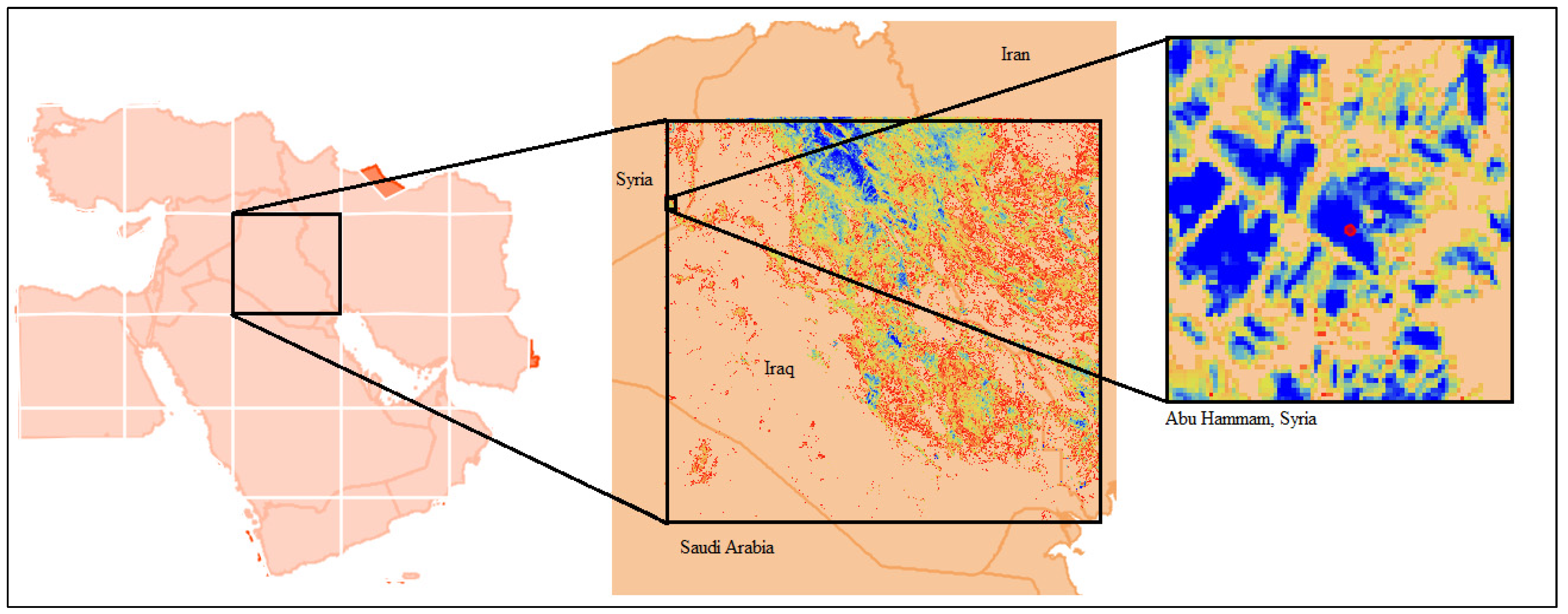
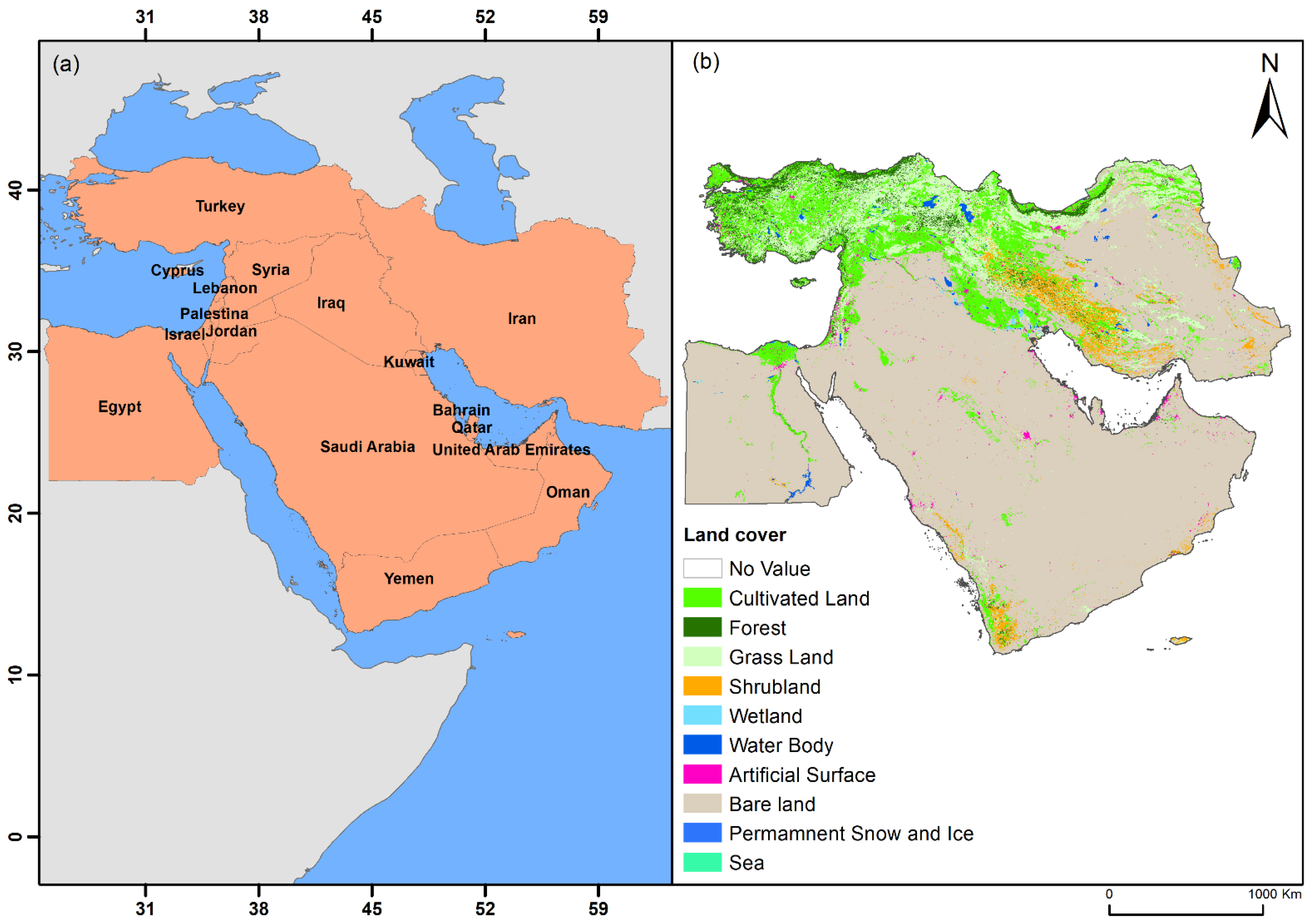
2.1. Study Area
2.2. Dataset
2.2.1. GlobeLand30
2.2.2. Landsat Land Surface Reflectance Data
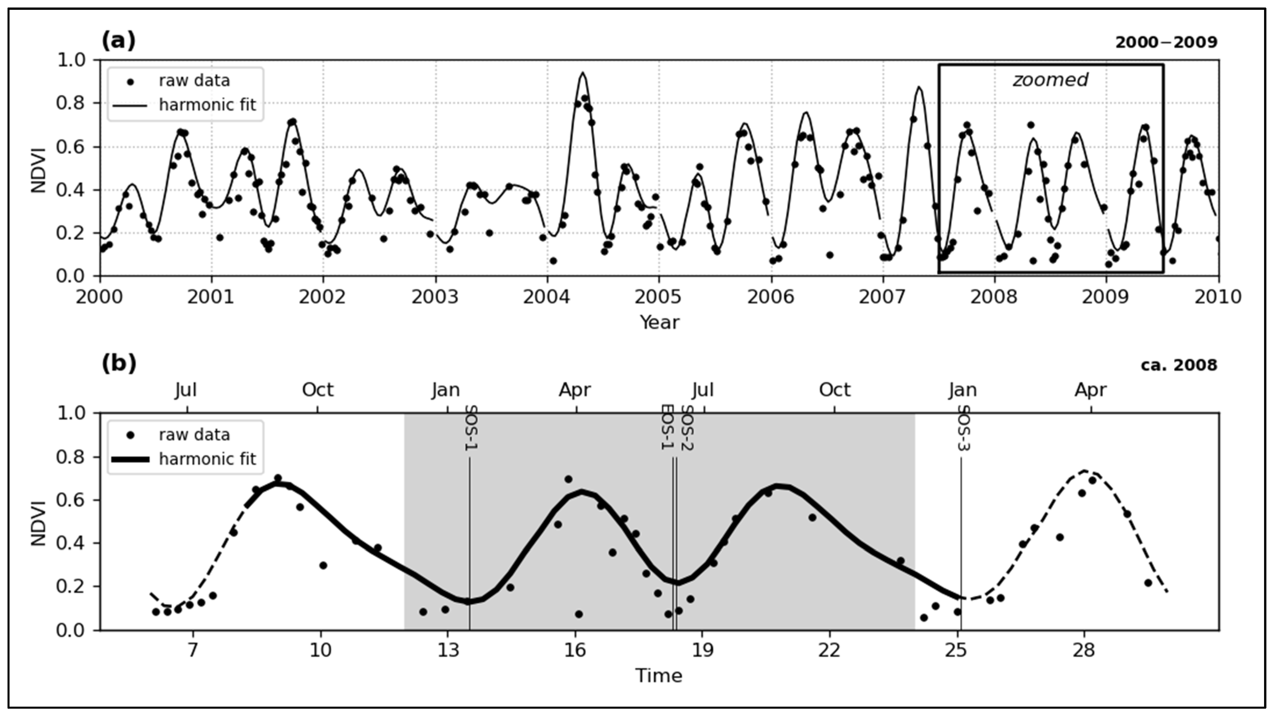
2.2.3. Phenology Extraction
2.2.4. Statistical Analysis
3. Results
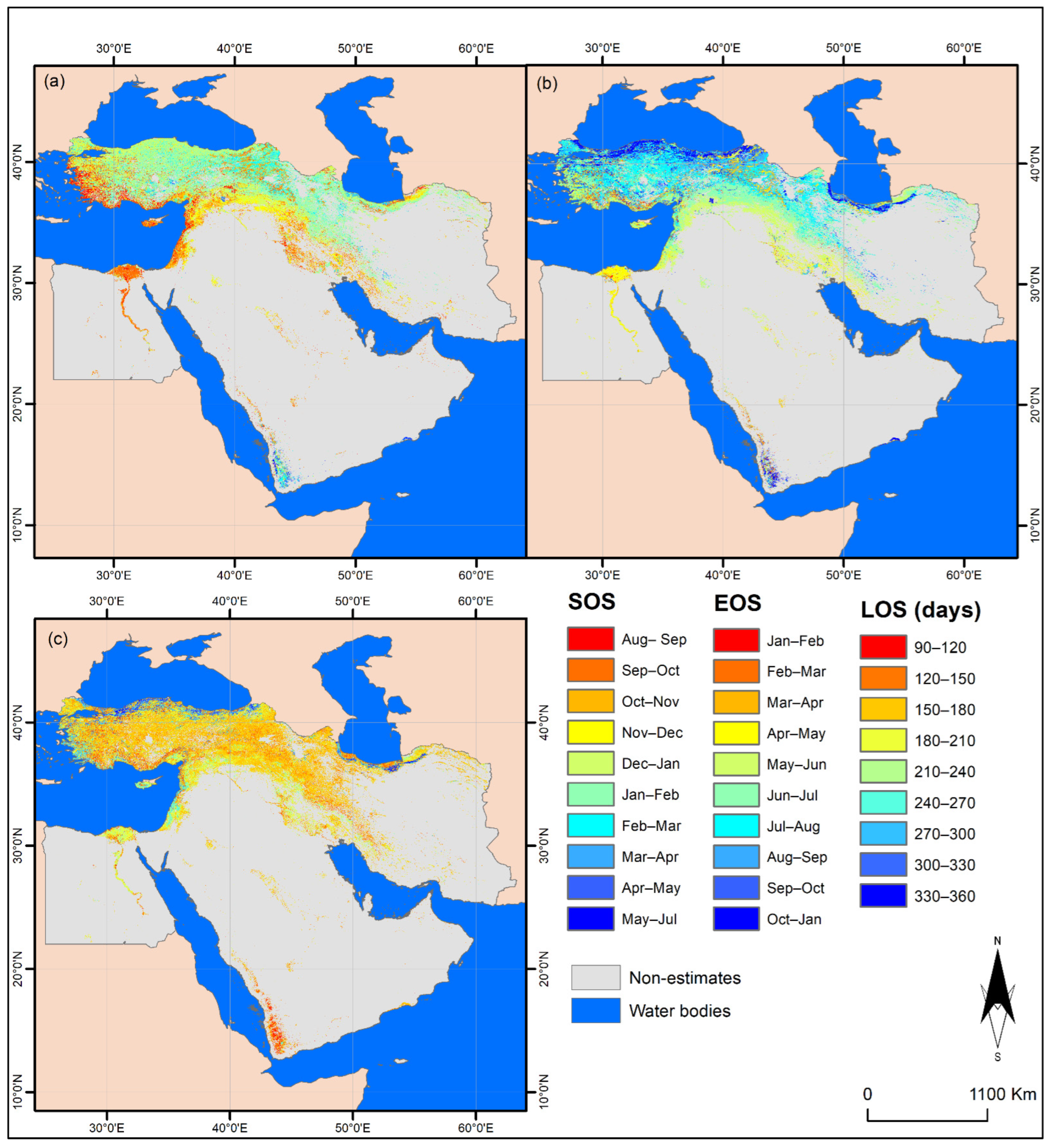
3.1. Spatiotemporal Variation in Phenological Parameters
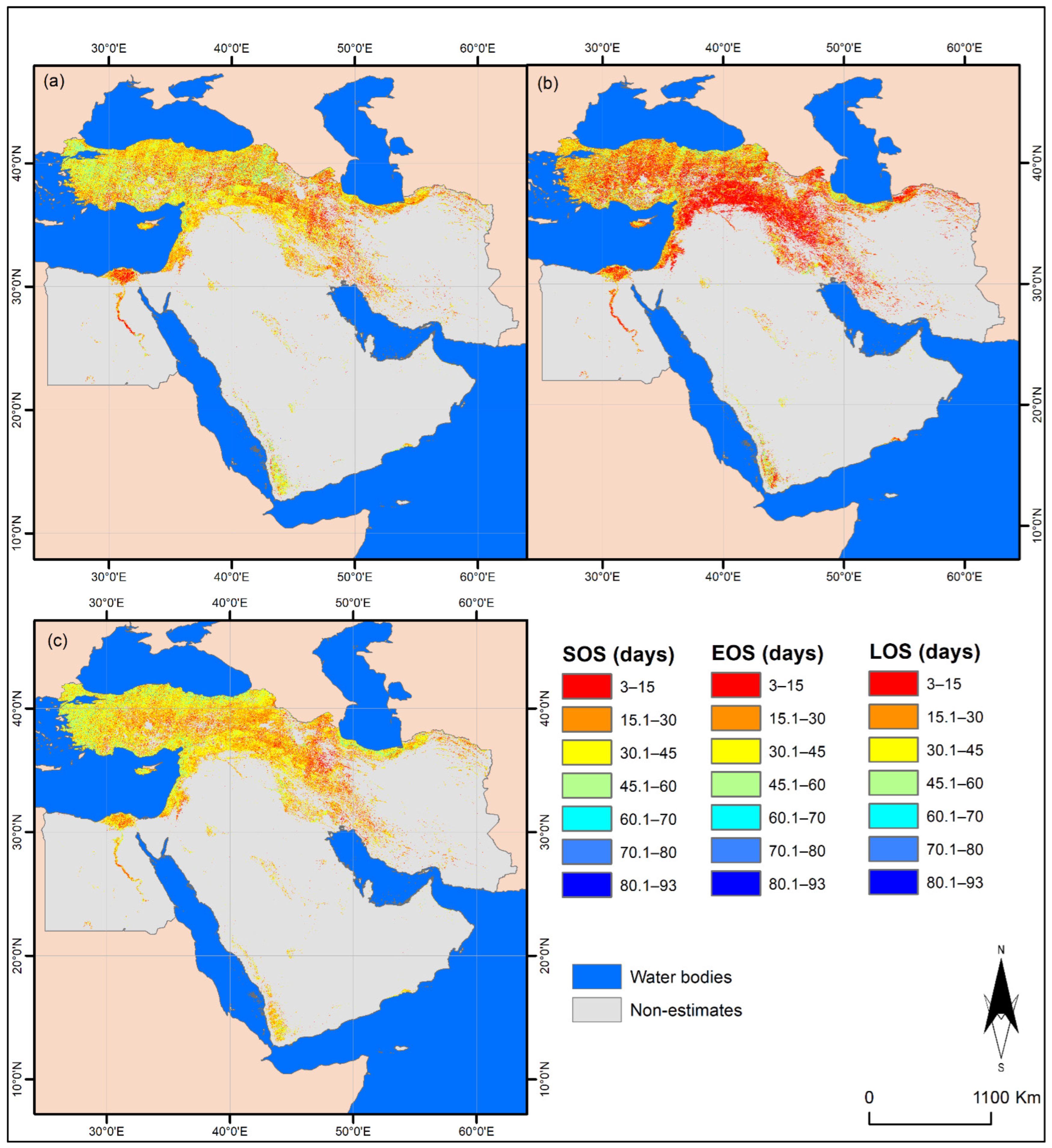
3.2. Variability in LSP Parameters
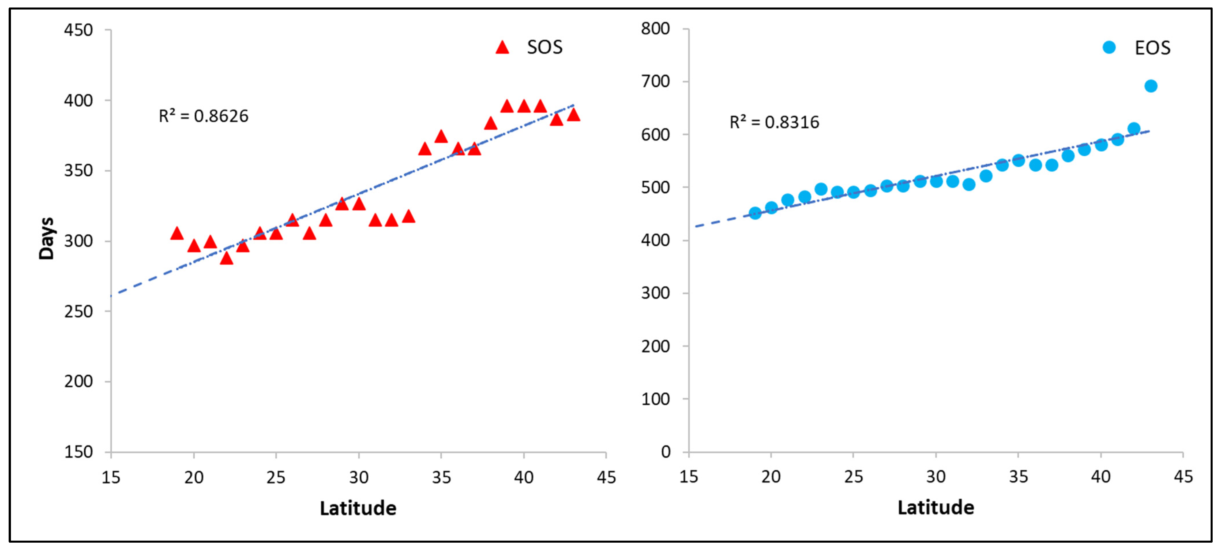
3.3. Latitudinal Variation of LSP Parameters
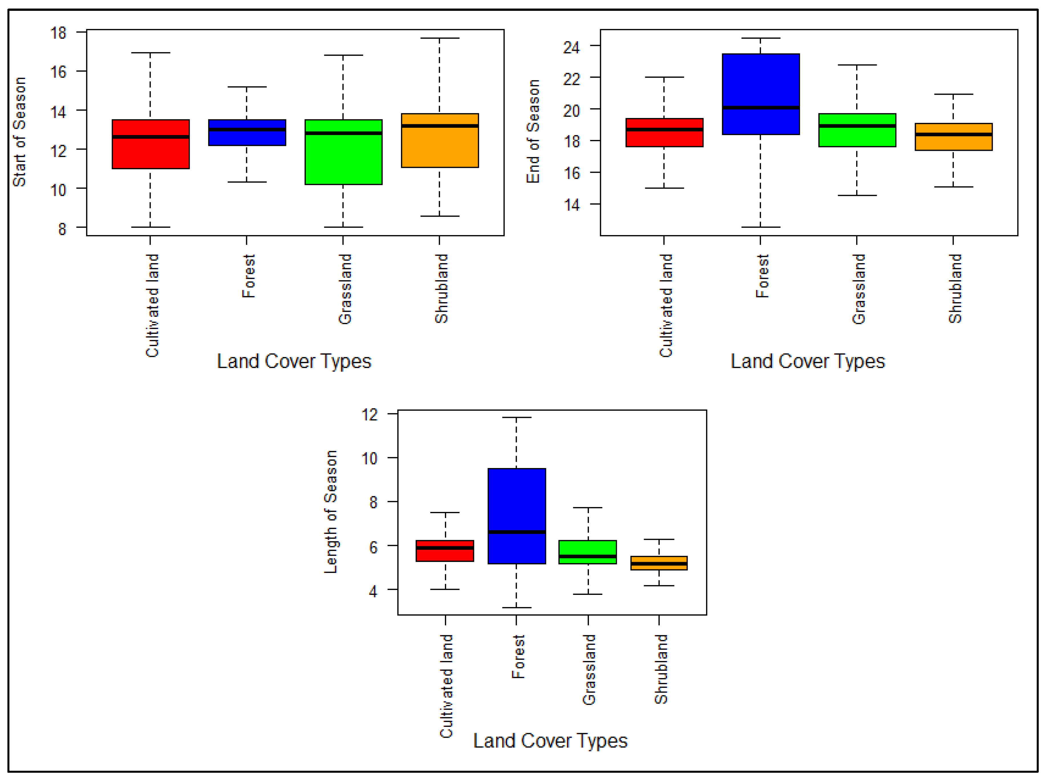
3.4. Characterising of the LSP of Major Land Cover Types in ME
4. Discussion
5. Conclusions
Author Contributions
Funding
Data Availability Statement
Conflicts of Interest
References
- Lieth, H. Phenology in productivity studies. In Analysis of Temperate Forest Ecosystems; Springer: Berlin/Heidelberg, Germany, 1973; pp. 29–46. [Google Scholar]
- Caparros-Santiago, J.A.; Rodriguez-Galiano, V.; Dash, J. Land surface phenology as indicator of global terrestrial ecosystem dynamics: A systematic review. ISPRS J. Photogramm. Remote Sens. 2021, 171, 330–347. [Google Scholar] [CrossRef]
- Menzel, A.; Sparks, T.H.; Estrella, N.; Koch, E.; Aasa, A.; Ahas, R.; Alm-Kübler, K.; Bissolli, P.; Braslavská, O.G.; Briede, A.; et al. European phenological response to climate change matches the warming pattern. Glob. Chang. Biol. 2006, 12, 1969–1976. [Google Scholar] [CrossRef]
- Parmesan, C.; Yohe, G. A globally coherent fingerprint of climate change impacts across natural systems. Nature 2003, 421, 37–42. [Google Scholar] [CrossRef] [PubMed]
- Qiu, T.; Song, C.; Zhang, Y.; Liu, H.; Vose, J.M. Urbanization and climate change jointly shift land surface phenology in the northern mid-latitude large cities. Remote Sens. Environ. 2020, 236, 111477. [Google Scholar] [CrossRef]
- Wolkovich, E.M.; Cook, B.I.; Allen, J.M.; Crimmins, T.M.; Betancourt, J.L.; Travers, S.E.; Pau, S.; Regetz, J.; Davies, T.J.; Kraft, N.J.; et al. Warming experiments underpredict plant phenological responses to climate change. Nature 2012, 485, 494–497. [Google Scholar] [CrossRef]
- Badeck, F.W.; Bondeau, A.; Böttcher, K.; Doktor, D.; Lucht, W.; Schaber, J.; Sitch, S. Responses of spring phenology to climate change. New Phytol. 2004, 162, 295–309. [Google Scholar] [CrossRef]
- Junttila, O.; Nilsen, J. Growth and development of northern forest trees as affected by temperature and light. In Forest Development in Cold Climates; Springer: Berlin/Heidelberg, Germany, 1993; pp. 43–57. [Google Scholar]
- Sobrino, J.A.; Julien, Y.; Morales, L. Changes in vegetation spring dates in the second half of the twentieth century. Int. J. Remote Sens. 2011, 32, 5247–5265. [Google Scholar] [CrossRef]
- Khwarahm, N.R. Mapping current and potential future distributions of the oak tree (Quercus aegilops) in the Kurdistan Region, Iraq. Ecol. Process. 2020, 9, 56. [Google Scholar] [CrossRef]
- Friedl, M.A.; Gray, J.M.; Melaas, E.K.; Richardson, A.D.; Hufkens, K.; Keenan, T.F.; Bailey, A.; O’Keefe, J. A tale of two springs: Using recent climate anomalies to characterize the sensitivity of temperate forest phenology to climate change. Environ. Res. Lett. 2014, 9, 054006. [Google Scholar] [CrossRef]
- Gao, X.; Gray, J.; Cohrs, C.W.; Cook, R.; Albaugh, T.J. Longer greenup periods associated with greater wood volume growth in managed pine stands. Agric. For. Meteorol. 2021, 297, 108237. [Google Scholar] [CrossRef]
- Piao, S.; Liu, Q.; Chen, A.; Janssens, I.A.; Fu, Y.; Dai, J.; Liu, L.; Lian, X.U.; Shen, M.; Zhu, X. Plant phenology and global climate change: Current progresses and challenges. Glob. Change Biol. 2019, 25, 1922–1940. [Google Scholar] [CrossRef] [PubMed]
- Richardson, A.D.; Keenan, T.F.; Migliavacca, M.; Ryu, Y.; Sonnentag, O.; Toomey, M. Climate change, phenology, and phenological control of vegetation feedbacks to the climate system. Agric. For. Meteorol. 2013, 169, 156–173. [Google Scholar] [CrossRef]
- Taylor, R.V.; Holthuijzen, W.; Humphrey, A.; Posthumus, E. Using phenology data to improve control of invasive plant species: A case study on Midway Atoll NWR. Ecol. Solut. Evid. 2020, 1, e12007. [Google Scholar] [CrossRef]
- Schwartz, M.D.; Betancourt, J.L.; Weltzin, J.F. From Caprio’s lilacs to the USA National Phenology Network. Front. Ecol. Environ. 2012, 10, 324–327. [Google Scholar] [CrossRef]
- Watson, C.J.; Restrepo-Coupe, N.; Huete, A.R. Multi-scale phenology of temperate grasslands: Improving monitoring and management with near-surface phenocams. Front. Environ. Sci. 2019, 7, 14. [Google Scholar] [CrossRef]
- Alberton, B.; Torres, R.D.; Cancian, L.F.; Borges, B.D.; Almeida, J.; Mariano, G.C.; dos Santos, J.; Morellato, L.P. Introducing digital cameras to monitor plant phenology in the tropics: Applications for conservation. Perspect. Ecol. Conserv. 2017, 15, 82–90. [Google Scholar] [CrossRef]
- Berra, E.F.; Gaulton, R.; Barr, S. Use of a digital camera onboard a UAV to monitor spring phenology at individual tree level. In Proceedings of the 2016 IEEE International Geoscience and Remote Sensing Symposium (IGARSS), Beijing, China, 10–15 July 2016; pp. 3496–3499. [Google Scholar]
- Assmann, J.J.; Myers-Smith, I.H.; Kerby, J.T.; Cunliffe, A.M.; Daskalova, G.N. Drone data reveal heterogeneity in tundra greenness and phenology not captured by satellites. Environ. Res. Lett. 2020, 15, 125002. [Google Scholar] [CrossRef]
- Qader, S.H.; Dash, J.; Alegana, V.A.; Khwarahm, N.R.; Tatem, A.J.; Atkinson, P.M. The Role of Earth Observation in Achieving Sustainable Agricultural Production in Arid and Semi-Arid Regions of the World. Remote Sens. 2021, 13, 3382. [Google Scholar] [CrossRef]
- Schwartz, M.D.; Reed, B.C. Surface phenology and satellite sensor-derived onset of greenness: An initial comparison. Int. J. Remote Sens. 1999, 20, 3451–3457. [Google Scholar] [CrossRef]
- Helman, D. Land surface phenology: What do we really ‘see’from space? Sci. Total Environ. 2018, 618, 665–673. [Google Scholar] [CrossRef]
- Zeng, L.; Wardlow, B.D.; Xiang, D.; Hu, S.; Li, D. A review of vegetation phenological metrics extraction using time-series, multispectral satellite data. Remote Sens. Environ. 2020, 237, 111511. [Google Scholar] [CrossRef]
- Davis, C.; Hoffman, M.; Roberts, W. Long-term trends in vegetation phenology and productivity over Namaqualand using the GIMMS AVHRR NDVI3g data from 1982 to 2011. South Afr. J. Bot. 2017, 111, 76–85. [Google Scholar] [CrossRef]
- Tong, X.; Tian, F.; Brandt, M.; Liu, Y.; Zhang, W.; Fensholt, R. Trends of land surface phenology derived from passive microwave and optical remote sensing systems and associated drivers across the dry tropics 1992–2012. Remote Sens. Environ. 2019, 232, 111307. [Google Scholar] [CrossRef]
- Nguyen, L.H.; Joshi, D.R.; Clay, D.E.; Henebry, G.M. Characterizing land cover/land use from multiple years of Landsat and MODIS time series: A novel approach using land surface phenology modeling and random forest classifier. Remote Sens. Environ. 2020, 238, 111017. [Google Scholar] [CrossRef]
- Tomaszewska, M.A.; Nguyen, L.H.; Henebry, G.M. Land surface phenology in the highland pastures of montane Central Asia: Interactions with snow cover seasonality and terrain characteristics. Remote Sens. Environ. 2020, 240, 111675. [Google Scholar] [CrossRef]
- Fontana, F.; Rixen, C.; Jonas, T.; Aberegg, G.; Wunderle, S. Alpine grassland phenology as seen in AVHRR, VEGETATION, and MODIS NDVI time series-a comparison with in situ measurements. Sensors 2008, 8, 2833–2853. [Google Scholar] [CrossRef] [Green Version]
- Weiss, E.; Marsh, S.; Pfirman, E. Application of NOAA-AVHRR NDVI time-series data to assess changes in Saudi Arabia’s rangelands. Int. J. Remote Sens. 2001, 22, 1005–1027. [Google Scholar] [CrossRef]
- Qader, S.H.; Atkinson, P.M.; Dash, J. Spatiotemporal variation in the terrestrial vegetation phenology of Iraq and its relation with elevation. Int. J. Appl. Earth Obs. Geoinf. 2015, 41, 107–117. [Google Scholar] [CrossRef]
- Gong, Z.; Kawamura, K.; Ishikawa, N.; Goto, M.; Wulan, T.; Alateng, D.; Yin, T.; Ito, Y. MODIS normalized difference vegetation index (NDVI) and vegetation phenology dynamics in the Inner Mongolia grassland. Solid Earth 2015, 6, 1185–1194. [Google Scholar] [CrossRef] [Green Version]
- Vrieling, A.; Meroni, M.; Darvishzadeh, R.; Skidmore, A.K.; Wang, T.; Zurita-Milla, R.; Oosterbeek, K.; O’Connor, B.; Paganini, M. Vegetation phenology from Sentinel-2 and field cameras for a Dutch barrier island. Remote Sens. Environ. 2018, 215, 517–529. [Google Scholar] [CrossRef]
- Tian, F.; Cai, Z.; Jin, H.; Hufkens, K.; Scheifinger, H.; Tagesson, T.; Eklundh, L. Calibrating vegetation phenology from Sentinel-2 using eddy covariance, PhenoCam, and PEP725 networks across Europe. Remote Sens. Environ. 2021, 260, 112456. [Google Scholar] [CrossRef]
- Dash, J.; Jeganathan, C.; Atkinson, P. The use of MERIS Terrestrial Chlorophyll Index to study spatio-temporal variation in vegetation phenology over India. Remote Sens. Environ. 2010, 114, 1388–1402. [Google Scholar] [CrossRef]
- Jeganathan, C.; Dash, J.; Atkinson, P.M. Characterising the spatial pattern of phenology for the tropical vegetation of India using multi-temporal MERIS chlorophyll data. Landsc. Ecol. 2010, 25, 1125–1141. [Google Scholar] [CrossRef]
- Rodriguez-Galiano, V.F.; Dash, J.; Atkinson, P.M. Characterising the land surface phenology of Europe using decadal MERIS data. Remote Sens. 2015, 7, 9390–9409. [Google Scholar] [CrossRef] [Green Version]
- Bornez, K.; Descals, A.; Verger, A.; Peñuelas, J. Land surface phenology from VEGETATION and PROBA-V data. Assessment over deciduous forests. Int. J. Appl. Earth Obs. Geoinf. 2020, 84, 101974. [Google Scholar] [CrossRef]
- Delbart, N.; Picard, G.; Le Toan, T.; Kergoat, L.; Quegan, S.; Woodward, I.A.; Dye, D.; Fedotova, V. Spring phenology in boreal Eurasia over a nearly century time scale. Glob. Change Biol. 2008, 14, 603–614. [Google Scholar] [CrossRef]
- Han, Q.; Luo, G.; Li, C. Remote sensing-based quantification of spatial variation in canopy phenology of four dominant tree species in Europe. J. Appl. Remote Sens. 2013, 7, 073485. [Google Scholar] [CrossRef] [Green Version]
- Shen, M.; Piao, S.; Dorji, T.; Liu, Q.; Cong, N.; Chen, X.; An, S.; Wang, S.; Wang, T.; Zhang, G. Plant phenological responses to climate change on the Tibetan Plateau: Research status and challenges. Natl. Sci. Rev. 2015, 2, 454–467. [Google Scholar] [CrossRef] [Green Version]
- Reed, B.C.; Brown, J.F.; VanderZee, D.; Loveland, T.R.; Merchant, J.W.; Ohlen, D.O. Measuring phenological variability from satellite imagery. J. Veg. Sci. 1994, 5, 703–714. [Google Scholar] [CrossRef]
- Viña, A.; Gitelson, A.A.; Nguy-Robertson, A.L.; Peng, Y. Comparison of different vegetation indices for the remote assessment of green leaf area index of crops. Remote Sens. Environ. 2011, 115, 3468–3478. [Google Scholar] [CrossRef]
- Wu, C.; Peng, D.; Soudani, K.; Siebicke, L.; Gough, C.M.; Arain, M.A.; Bohrer, G.; Lafleur, P.M.; Peichl, M.; Gonsamo, A.; et al. Land surface phenology derived from normalized difference vegetation index (NDVI) at global FLUXNET sites. Agric. For. Meteorol. 2017, 233, 171–182. [Google Scholar] [CrossRef]
- Huete, A.; Didan, K.; Miura, T.; Rodriguez, E.P.; Gao, X.; Ferreira, L.G. Overview of the radiometric and biophysical performance of the MODIS vegetation indices. Remote Sens. Environ. 2002, 83, 195–213. [Google Scholar] [CrossRef]
- Maignan, F.; Bréon, F.-M.; Bacour, C.; Demarty, J.; Poirson, A. Interannual vegetation phenology estimates from global AVHRR measurements: Comparison with in situ data and applications. Remote Sens. Environ. 2008, 112, 496–505. [Google Scholar] [CrossRef]
- Khwarahm, N.R.; Dash, J.; Skjøth, C.A.; Newnham, R.M.; Adams-Groom, B.; Head, K.; Caulton, E.; Atkinson, P.M. Mapping the birch and grass pollen seasons in the UK using satellite sensor time-series. Sci. Total Environ. 2017, 578, 586–600. [Google Scholar] [CrossRef] [Green Version]
- Wang, C.; Chen, J.; Wu, J.; Tang, Y.; Shi, P.; Black, T.A.; Zhu, K. A snow-free vegetation index for improved monitoring of vegetation spring green-up date in deciduous ecosystems. Remote Sens. Environ. 2017, 196, 1–12. [Google Scholar] [CrossRef]
- Abbas, N.; Wasimi, S.A.; Al-Ansari, N.; Nasrin Baby, S. Recent trends and long-range forecasts of water resources of northeast Iraq and climate change adaptation measures. Water 2018, 10, 1562. [Google Scholar] [CrossRef] [Green Version]
- Ahmadalipour, A.; Moradkhani, H. Escalating heat-stress mortality risk due to global warming in the Middle East and North Africa (MENA). Environ. Int. 2018, 117, 215–225. [Google Scholar] [CrossRef]
- Hameed, M.; Ahmadalipour, A.; Moradkhani, H. Apprehensive drought characteristics over Iraq: Results of a multidecadal spatiotemporal assessment. Geosciences 2018, 8, 58. [Google Scholar] [CrossRef] [Green Version]
- Tolba, M.K.S.; Najib, W. Arab Environment: Climate Change: Impact of Climate Change on Arab Countries; Arab Forum for Environment and Development (AFED): Beirut, Lebanon, 2009. [Google Scholar]
- Hameed, M.; Ahmadalipour, A.; Moradkhani, H. Drought and food security in the middle east: An analytical framework. Agric. For. Meteorol. 2020, 281, 107816. [Google Scholar] [CrossRef]
- Lelieveld, J.; Hadjinicolaou, P.; Kostopoulou, E.; Chenoweth, J.; El Maayar, M.; Giannakopoulos, C.; Hannides, C.; Lange, M.A.; Tanarhte, M.; Tyrlis, E.; et al. Climate change and impacts in the Eastern Mediterranean and the Middle East. Clim. Change 2012, 114, 667–687. [Google Scholar] [CrossRef] [Green Version]
- Evans, J.; Geerken, R. Discrimination between climate and human-induced dryland degradation. J. Arid Environ. 2004, 57, 535–554. [Google Scholar] [CrossRef]
- Qader, S.H.; Dash, J.; Atkinson, P.M. Forecasting wheat and barley crop production in arid and semi-arid regions using remotely sensed primary productivity and crop phenology: A case study in Iraq. Sci. Total Environ. 2018, 613, 250–262. [Google Scholar] [CrossRef] [Green Version]
- Daham, A.; Han, D.; Matt Jolly, W.; Rico-Ramirez, M.; Marsh, A. Predicting vegetation phenology in response to climate change using bioclimatic indices in Iraq. J. Water Clim. Chang. 2019, 10, 835–851. [Google Scholar] [CrossRef]
- Qader, S.H.; Dash, J.; Atkinson, P.M.; Rodriguez-Galiano, V. Classification of vegetation type in Iraq using satellite-based phenological parameters. IEEE J. Sel. Top. Appl. Earth Obs. Remote Sens. 2016, 9, 414–424. [Google Scholar] [CrossRef]
- Eklund, L.; Persson, A.; Tang, J.; Selander, M.; Borg, M. Using Crop Phenology to Assess Changes in Cultivated Land after the Anfal Genocide in Iraqi Kurdistan. 2014. Available online: https://agile-online.org/conference_paper/cds/agile_2014/agile2014_113.pdf (accessed on 25 February 2022).
- Araghi, A.; Martinez, C.J.; Adamowski, J.; Olesen, J.E. Associations between large-scale climate oscillations and land surface phenology in Iran. Agric. For. Meteorol. 2019, 278, 107682. [Google Scholar] [CrossRef]
- Kiapasha, K.; Darvishsefat, A.A.; Julien, Y.; Sobrino, J.A.; Zargham, N.; Attarod, P.; Schaepman, M.E. Trends in Phenological Parameters and Relationship Between Land Surface Phenology and Climate Data in the Hyrcanian Forests of Iran. IEEE J. Sel. Top. Appl. Earth Obs. Remote Sens. 2017, 10, 4961–4970. [Google Scholar] [CrossRef]
- Padhee, S.K.; Dutta, S. Spatio-temporal reconstruction of MODIS NDVI by regional land surface phenology and harmonic analysis of time-series. GIScience Remote Sens. 2019, 56, 1261–1288. [Google Scholar] [CrossRef]
- Evrendilek, F.; Gulbeyaz, O. Deriving vegetation dynamics of natural terrestrial ecosystems from MODIS NDVI/EVI data over Turkey. Sensors 2008, 8, 5270–5302. [Google Scholar] [CrossRef] [Green Version]
- Mermer, A.; Yıldız, H.; Ünal, E.; Aydoğdu, M.; Özaydın, A.; Dedeoğlu, F.; Urla, O.; Aydoğmuş, O.; Torunlar, H.; Tuğaç, M.; et al. Monitoring rangeland vegetation through time series satellite images (NDVI) in Central Anatolia Region. In Proceedings of the 2015 Fourth International Conference on Agro-Geoinformatics (Agro-Geoinformatics), Istanbul, Turkey, 20–24 July 2015; pp. 213–216. [Google Scholar]
- Soudani, K.; Hmimina, G.; Delpierre, N.; Pontailler, J.Y.; Aubinet, M.; Bonal, D.; Caquet, B.; De Grandcourt, A.; Burban, B.; Flechard, C.; et al. Ground-based Network of NDVI measurements for tracking temporal dynamics of canopy structure and vegetation phenology in different biomes. Remote Sens. Environ. 2012, 123, 234–245. [Google Scholar] [CrossRef]
- Yıldırım, T.; Aşık, Ş. Index-based assessment of agricultural drought using remote sensing in the semi-arid region of Western Turkey. J. Agric. Sci. 2018, 24, 510–516. [Google Scholar]
- Farg, E.; Ramadan, M.N.; Arafat, S.M. Classification of some strategic crops in Egypt using multi remotely sensing sensors and time series analysis. Egypt. J. Remote Sens. Space Sci. 2019, 22, 263–270. [Google Scholar] [CrossRef]
- Xu, Y.; Yu, L.; Zhao, Y.; Feng, D.; Cheng, Y.; Cai, X.; Gong, P. Monitoring cropland changes along the Nile River in Egypt over past three decades (1984–2015) using remote sensing. Int. J. Remote Sens. 2017, 38, 4459–4480. [Google Scholar] [CrossRef]
- Makhamreh, Z. Derivation of vegetation density and land-use type pattern in mountain regions of Jordan using multi-seasonal SPOT images. Environ. Earth Sci. 2018, 77, 384. [Google Scholar] [CrossRef]
- Saba, M.; Al-Naber, G.; Mohawesh, Y. Analysis of Jordan vegetation cover dynamics using MODIS/NDVI from 2000 to 2009. In Food Security and Climate Change in Dry Areas, Proceedings of the an International Conference, Amman, Jordan, 1–4 February 2010; International Center for Agricultural Research in the Dry Areas: Aleppo, Syria, 2011; p. 79. [Google Scholar]
- Argaman, E.; Barth, R.; Moshe, Y.; Ben-Hur, M. Long-term effects of climatic and hydrological variation on natural vegetation production and characteristics in a semiarid watershed: The northern Negev, Israel. Sci. Total Environ. 2020, 747, 141146. [Google Scholar] [CrossRef]
- Schmidt, H.; Gitelson, A. Temporal and spatial vegetation cover changes in Israeli transition zone: AVHRR-based assessment of rainfall impact. Int. J. Remote Sens. 2000, 21, 997–1010. [Google Scholar] [CrossRef]
- Abd El-Ghani, M.M. Phenology of ten common plant species in western Saudi Arabia. J. Arid. Environ. 1997, 35, 673–683. [Google Scholar] [CrossRef]
- Bunker, B.E.; Tullis, J.A.; Cothren, J.D.; Casana, J.; Aly, M.H. Object-based dimensionality reduction in land surface phenology classification AIMS. Geosciences 2016, 2, 302–328. [Google Scholar]
- World Atlas. How Many Countries Are There In the Middle East? 2022. Available online: https://www.worldatlas.com/articles/which-are-the-middle-eastern-countries.html#:~:text=Middle%20East%20includes%2018%20countries,United%20Arab%20Emirates%20and%20Yemen (accessed on 7 February 2022).
- Zaitchik, B.F.; Evans, J.P.; Geerken, R.A.; Smith, R.B. Climate and vegetation in the Middle East: Interannual variability and drought feedbacks. J. Clim. 2007, 20, 3924–3941. [Google Scholar] [CrossRef]
- GlobeLand30. Global Land Cover Mapping at 30 m Resolution (2020). 2022. Available online: http://www.globallandcover.com/ (accessed on 11 January 2022).
- DIVA-GIS. Free Spatial Data by Country. 2022. Available online: https://www.diva-gis.org/gdata (accessed on 12 December 2021).
- Jun, C.; Ban, Y.; Li, S. Open access to Earth land-cover map. Nature 2014, 514, 434. [Google Scholar] [CrossRef] [Green Version]
- Gorelick, N.; Hancher, M.; Dixon, M.; Ilyushchenko, S.; Thau, D.; Moore, R. Google Earth Engine: Planetary-scale geospatial analysis for everyone. Remote Sens. Environ. 2017, 202, 18–27. [Google Scholar] [CrossRef]
- Kovalsky, V.; Roy, D.P. The global availability of Landsat 5 TM and Landsat 7 ETM + land surface observations and implications for global 30 m Landsat data product generation. Remote Sens. Environ. 2013, 130, 280–293. [Google Scholar] [CrossRef] [Green Version]
- Markham, B.L.; Storey, J.C.; Williams, D.L.; Irons, J.R. Landsat sensor performance: History and current status. IEEE Trans. Geosci. Remote Sens. 2004, 42, 2691–2694. [Google Scholar] [CrossRef]
- Teillet, P.M.; Barker, J.L.; Markham, B.L.; Irish, R.R.; Fedosejevs, G.; Storey, J.C. Radiometric cross-calibration of the Landsat-7 ETM+ and Landsat-5 TM sensors based on tandem data sets. Remote Sens. Environ. 2001, 78, 39–54. [Google Scholar] [CrossRef] [Green Version]
- Ardvison, T.; Goward, S.; Gasch, J.; Williams, D. Landsat-7 long-term acquisition plan: Development and validation. Photogramm. Eng. Remote Sens. 2006, 72, 1137–1146. [Google Scholar]
- Chen, J.; Zhu, X.; Vogelmann, J.E.; Gao, F.; Jin, S. A simple and effective method for filling gaps in Landsat ETM + SLC-off images. Remote Sens. Environ. 2011, 115, 1053–1064. [Google Scholar] [CrossRef]
- Rouse, J.W.; Haas, R.H.; Schell, J.A.; Deering, W.D. Monitoring vegetation systems in the Great Plains with ERTS. In Proceedings of the Third ERTS Symposium, NASA SP–351, Washington, DC, USA, 10–14 December 1973; pp. 309–317. [Google Scholar]
- Schmidt, G.; Jenkerson, C.B.; Masek, J.; Vermote, E.; Gao, F. Landsat Ecosystem Disturbance Adaptive Processing System (LEDAPS) Algorithm Description; Technical Report; U.S. Geological Survey: Sioux Falls, SD, USA, 2013. [Google Scholar]
- Foga, S.; Scaramuzza, P.L.; Guo, S.; Zhu, Z.; Dilley, R.D.; Beckmann, T.; Schmidt, G.L.; Dwyer, J.L.; Hughes, M.J.; Laue, B. Cloud detection algorithm comparison and validation for operational Landsat data products. Remote Sens. Environ. 2017, 194, 379–390. [Google Scholar] [CrossRef] [Green Version]
- Jakubauskas, M.E.; Legates, D.R.; Kastens, J.H. Harmonic analysis of time-series AVHRR NDVI data. Photogramm. Eng. Remote Sens. 2001, 67, 461–470. [Google Scholar]
- Wagenseil, H.; Samimi, C. Assessing spatio–temporal variations in plant phenology using Fourier analysis on NDVI time series: Results from a dry savannah environment in Namibia. Int. J. Remote Sens. 2006, 27, 3455–3471. [Google Scholar] [CrossRef]
- Tedla, B.; Dang, Q.-L.; Inoue, S. CO2 Elevation and Photoperiods North of Seed Origin Change Autumn and Spring Phenology as Well as Cold Hardiness in Boreal White Birch. Front. Plant Sci. 2020, 11, 506. [Google Scholar] [CrossRef]
- Wang, X.; Wu, C.; Zhang, X.; Li, Z.; Liu, Z.; Gonsamo, A.; Ge, Q. Satellite-observed decrease in the sensitivity of spring phenology to climate change under high nitrogen deposition. Environ. Res. Lett. 2020, 15, 094055. [Google Scholar] [CrossRef]
- Roy, D.P.; Kovalskyy, V.; Zhang, H.K.; Vermote, E.F.; Yan, L.; Kumar, S.S.; Egorov, A. Characterization of Landsat-7 to Landsat-8 reflective wavelength and normalized difference vegetation index continuity. Remote Sens. Environ. 2016, 185, 57–70. [Google Scholar] [CrossRef] [PubMed] [Green Version]
- Mancino, G.; Ferrara, A.; Padula, A.; Nolè, A. Cross-Comparison between Landsat 8 (OLI) and Landsat 7 (ETM+) Derived Vegetation Indices in a Mediterranean Environment. Remote Sens. 2020, 12, 291. [Google Scholar] [CrossRef] [Green Version]
- Friedl, M.; Gray, J.; Sulla-Menashe, D. MCD12Q2 MODIS/Terra+Aqua Land Cover Dynamics Yearly L3 Global 500 m SIN Grid V006 [Data Set]; NASA EOSDIS Land Processes DAAC. 2019. Available online: https://doi.org/10.5067/MODIS/MCD12Q2.006(accessed on 25 February 2022).
- Cleverly, J.; Eamus, D.; Restrepo Coupe, N.; Chen, C.; Maes, W.; Li, L.; Huete, A. Soil moisture controls on phenology and productivity in a semi-arid critical zone. Sci. Total Environ. 2016, 568, 1227–1237. [Google Scholar] [CrossRef] [PubMed]
- Wang, C.; Beringer, J.; Hutley, L.B.; Cleverly, J.; Li, J.; Liu, Q.; Sun, Y. Phenology Dynamics of Dryland Ecosystems along North Australian Tropical Transect Revealed by Satellite Solar-Induced Chlorophyll Fluorescence. Geophys. Res. Lett. 2019, 46, 5294–5302. [Google Scholar] [CrossRef]
- Cui, L.; Shi, J. Evaluation and comparison of growing season metrics in arid and semi-arid areas of northern China under climate change. Ecol. Indic. 2021, 121, 107055. [Google Scholar] [CrossRef]
- Xie, Q.; Cleverly, J.; Moore, C.E.; Ding, Y.; Hall, C.C.; Ma, X.; Huete, A. Land surface phenology retrievals for arid and semi-arid ecosystems. ISPRS J. Photogramm. Remote Sens. 2022, 185, 129–145. [Google Scholar] [CrossRef]
- Xie, Y.; Sha, Z.; Yu, M. Remote sensing imagery in vegetation mapping: A review. J. Plant Ecol. 2008, 1, 9–23. [Google Scholar] [CrossRef]
- Curran, M.F.; Hodza, P.; Cox, S.E.; Lanning, S.G.; Robertson, B.L.; Robinson, T.J.; Stahl, P.D. Ground-level Unmanned Aerial System Imagery Coupled with Spatially Balanced Sampling and Route Optimization to Monitor Rangeland Vegetation. J. Vis. Exp. 2020, 160, e61052. [Google Scholar] [CrossRef] [PubMed]
- Reed, B.C.; White, M.; Brown, J.F. Remote Sensing Phenology. In Phenology: An Integrative Environmental Science. Tasks for Vegetation Science; Schwartz, M.D., Ed.; Springer: Dordrecht, The Netherlands, 2003; Volume 39. [Google Scholar] [CrossRef]
- Matongera, T.N.; Mutanga, O.; Sibanda, M.; Odindi, J. Estimating and Monitoring Land Surface Phenology in Rangelands: A Review of Progress and Challenges. Remote Sens. 2021, 13, 2060. [Google Scholar] [CrossRef]
- Jokar Arsanjani, J.; Tayyebi, A.; Vaz, E. GlobeLand30 as an alternative fine-scale global land cover map: Challenges, possibilities, and implications for developing countries. Habitat Int. 2016, 55, 25–31. [Google Scholar] [CrossRef]
- Sun, B.; Chen, X.; Zhou, Q. Uncertainty assessment of GlobeLand30 land cover data set over central Asia. Int. Arch. Photogramm. Remote Sens. Spat. Inf. Sci. 2016, 41, 1313–1317. [Google Scholar] [CrossRef] [Green Version]
- Günşen, H.B.; Atmiş, E. Analysis of forest change and deforestation in Turkey. Int. For. Rev. 2019, 21, 182–194. [Google Scholar] [CrossRef]
- Coşgun, U.; González-Cabán, A. Factors explaining forest fires in the Serik and Taşağıl forest provinces (SW Anatolia-Turkey). In Proceedings of the Fifth International Symposium on Fire Economics, Planning, and Policy: Ecosystem Services and Wildfires; General Technical Report PNW-GTR-261; USDA Department of Agriculture, Forest Service, Pacific Southwest Research Station: Albany, CA, USA, 2019; pp. 145–165. [Google Scholar]
- Peng, D.; Wang, Y.; Xian, G.; Huete, A.R.; Huang, W.; Shen, M.; Zhang, X. Investigation of land surface phenology detections in shrublands using multiple scale satellite data. Remote Sens. Environ. 2021, 252, 112133. [Google Scholar] [CrossRef]
- Schnepf, R. Iraq Agriculture and Food Supply: Background and Issues, Congressional Research Service; The Library of Congress: Washington, DC, USA, 2004; pp. 9–10. [Google Scholar]
- Gibson, G.R.; Campbell, J.B.; Wynne, R.H. Three decades of war and food insecurity in Iraq. Photogramm. Eng. Remote Sens. 2012, 78, 885–895. [Google Scholar] [CrossRef]
- Adole, T.; Dash, J.; Atkinson, P.M. Characterising the land surface phenology of Africa using 500 m MODIS EVI. Appl. Geogr. 2018, 90, 187–199. [Google Scholar] [CrossRef] [Green Version]


| Parameter | Description |
|---|---|
| Start of season (SOS) | Valid valley before the peak of season |
| Peak of season (tmax) | Time at which NDVI reaches maximum in a single year |
| End of season (EOS) | Valid valley after the peak of season |
| Length of season (LOS) | Time difference between EOS and SOS |
| Maximum NDVI | Maximum value of NDVI between SOS and EOS |
| LSP Parameters | R2 | Slop | y-Intercept | p (Sig.) |
|---|---|---|---|---|
| SOS | 0.86 | 4.83 | 188.6 | <0.0001 |
| EOS | 0.83 | 6.54 | 325.89 | <0.0001 |
Publisher’s Note: MDPI stays neutral with regard to jurisdictional claims in published maps and institutional affiliations. |
© 2022 by the authors. Licensee MDPI, Basel, Switzerland. This article is an open access article distributed under the terms and conditions of the Creative Commons Attribution (CC BY) license (https://creativecommons.org/licenses/by/4.0/).
Share and Cite
Qader, S.H.; Priyatikanto, R.; Khwarahm, N.R.; Tatem, A.J.; Dash, J. Characterising the Land Surface Phenology of Middle Eastern Countries Using Moderate Resolution Landsat Data. Remote Sens. 2022, 14, 2136. https://doi.org/10.3390/rs14092136
Qader SH, Priyatikanto R, Khwarahm NR, Tatem AJ, Dash J. Characterising the Land Surface Phenology of Middle Eastern Countries Using Moderate Resolution Landsat Data. Remote Sensing. 2022; 14(9):2136. https://doi.org/10.3390/rs14092136
Chicago/Turabian StyleQader, Sarchil Hama, Rhorom Priyatikanto, Nabaz R. Khwarahm, Andrew J. Tatem, and Jadunandan Dash. 2022. "Characterising the Land Surface Phenology of Middle Eastern Countries Using Moderate Resolution Landsat Data" Remote Sensing 14, no. 9: 2136. https://doi.org/10.3390/rs14092136
APA StyleQader, S. H., Priyatikanto, R., Khwarahm, N. R., Tatem, A. J., & Dash, J. (2022). Characterising the Land Surface Phenology of Middle Eastern Countries Using Moderate Resolution Landsat Data. Remote Sensing, 14(9), 2136. https://doi.org/10.3390/rs14092136