Decadal Changes in Greenland Ice Sheet Firn Aquifers from Radar Scatterometer

Abstract

Surface meltwater runoff is believed to be the main cause of the alarming mass loss in the Greenland Ice Sheet (GrIS); however, recent research has shown that a large amount of meltwater is not directly drained or refrozen but stored in the form of firn aquifers (FAs) in the interior of the GrIS. Monitoring the changes in FAs over the GrIS is of great importance to evaluate the stability and mass balance of the ice sheet. This is challenging because FAs are not visible on the surface and the direct measurements are lacking. A new method is proposed to map FAs during the 2010–2020 period by using the C-band Advanced Scatterometer (ASCAT) data based on the Random Forests classification algorithm with the aid of measurements from the NASA Operation IceBridge (OIB) program. Melt days (MD), melt intensity (MI), and winter mean backscatter (WM) parameters derived from the ASCAT data are used as the input vectors for the Random Forests classification algorithm. The accuracy of the classification model is assessed by ten-fold cross-validation, and the overall accuracy and Kappa coefficient are 97.49% and 0.72 respectively. The results show that FAs reached the maximum in 2015, and the accumulative area of FAs from 2010 to 2020 is 56,477 km², which is 3.3% of the GrIS area. This study provides a way to investigate the long-term dynamics in FAs which have great significance for understanding the state of subsurface firn and subglacial hydrological systems.

1. Introduction

The disintegration of the overflow glaciers and the melting of the ice sheet surface are the two main causes of mass loss of the Greenland Ice Sheet (GrIS) [1,2,3,4]. Due to the melt-albedo feedback, surface meltwater formed by the warming of ice and snow layers heats up fast and accelerates the melting of surrounding ice and snow. When surface meltwater travels through the supraglacial, englacial, and subglacial hydrologic system to the bottom of the ice sheet, it lubricates the ice body and accelerates ice flow velocity, which may contribute to the calving of the overflowing glaciers [1,5,6]. Surface meltwater and its influence on the mass balance and sea-level rise have become the focus of GrIS research in recent years [7,8,9]. Recent research shows that the surface meltwater runoff contributed to 50.3% of the GrIS mass loss from 1992 to 2018 [10]. In addition, many studies have shown that meltwater may drain via a hydrofracture or refreeze in near-surface firn in the percolation zone, while some meltwater may remain in liquid form in the firn through the winter [11,12,13].

Firn aquifers (FAs) were first discovered in 2011 by analyzing the firn cores collected in Helheim Glacier of the southeast GrIS during the Arctic Circle Traverse expedition [14]. FAs form when summer meltwater percolates into the pores of the firn and liquid water persists throughout the following winter [14]. FAs occur in areas with strong surface melting and high snow accumulation which can insulate the cold air and prevent liquid water from refreezing [15,16,17,18]. Recent studies have found FAs in the southeast, south, and northwest of the GrIS and Wilkins Ice Shelf of the Antarctic Peninsula [15,16].

FAs can affect the thermal state of the underlying ice beneath aquifers, the hydrofracturing of ice shelves, and may indirectly affect the sea-level rise. When liquid water contained in FAs freezes, the released heat warms the surrounding firn and ice and further delays the subsequent freezing [14,19]. The meltwater stored in FAs may flow into cracks, crevasses, or rifts through the subglacial hydrologic system, increasing fracture depth, flowing to the bed of the ice sheet, and leading to ice shelf destabilization, which provides a potential mechanism for aquifer drainage and impacts ice dynamics [20,21]. The FAs system may serve as a temporary buffer against sea-level rise assuming the volume of FAs is stable [22]. However, if the FAs adjust their volume storage in response to the change with surface force, then the periodic release of the stored water from the aquifers to the ocean can potentially contribute to sea-level rise [21,23].

A variety of field measurements, including density, temperature, and hydraulic conductivity, were used to study FAs based on the core-drilling method [15,18,22,24,25]. The seismic refraction and ground-penetrating radar (GPR) experiments were implemented to identify the water table depth and aquifers’ thickness [15,26,27,28]. By using airborne radar and satellite measurements, the FAs extent was estimated [29,30,31,32,33]. Meanwhile, the firn models and regional climate models were used to explain the formation mechanism and predict the distribution of FAs [16,17,34]. Results from field measurements and firn models also supported the presence of FAs on the Wilkins Ice Shelf, which has comparable amounts of summer surface melt and snow accumulation with the GrIS [15,16].

Space-borne remote sensing datasets and methods have recently been applied to map FAs, considering the limitations of detection extent and time in field measurements and airborne radar observations, the uncertainties of physical process description, and the low-quality of input parameters in the model simulation. According to a distinctive pattern in the radar backscatter time series caused by the delay in the freezing of meltwater within the firn above the water table, Brangers et al. [31] used Sentinel-1 radar backscatter to map the FAs across the GrIS at 1 km resolution from 2014 to 2019. However, the Sentinel-1 firn aquifers detection relies on multiyear average September and April measurements and the empirical threshold method [31]. It assumes that FAs locations are stable in time which is unable to monitor the temporal changes in aquifer presence and extent [31]. Based on the exponential decrease of FAs in the L-band brightness temperature signatures of the Soil Moisture Active Passive (SMAP) satellite data, Miller et al. [33] mapped the FAs extent by fitting these signatures to a set of sigmoidal curves during 2015–2019. However, the SMAP-derived parameters are not exactly coincident with airborne ice-penetrating radar detections in time and the distinct temporal L-band signature lacks delineation of the boundary between firn aquifers areas, ice slabs areas, and adjacent percolation facies areas [33].

In this study, with the aid of measurements from the NASA Operation IceBridge (OIB) program, the active microwave enhanced-resolution Advanced Scatterometer (ASCAT) data from 2007 to 2020 is utilized to investigate the dynamic in FAs over the GrIS. Section 2.1 introduces the scatterometer data and the FAs dataset detected from the OIB program. Section 2.2 describes the detection method using the Random Forests (RF) classification algorithm. In Section 3 and Section 4, we show the results and the discussions respectively.

2. Materials and Methods

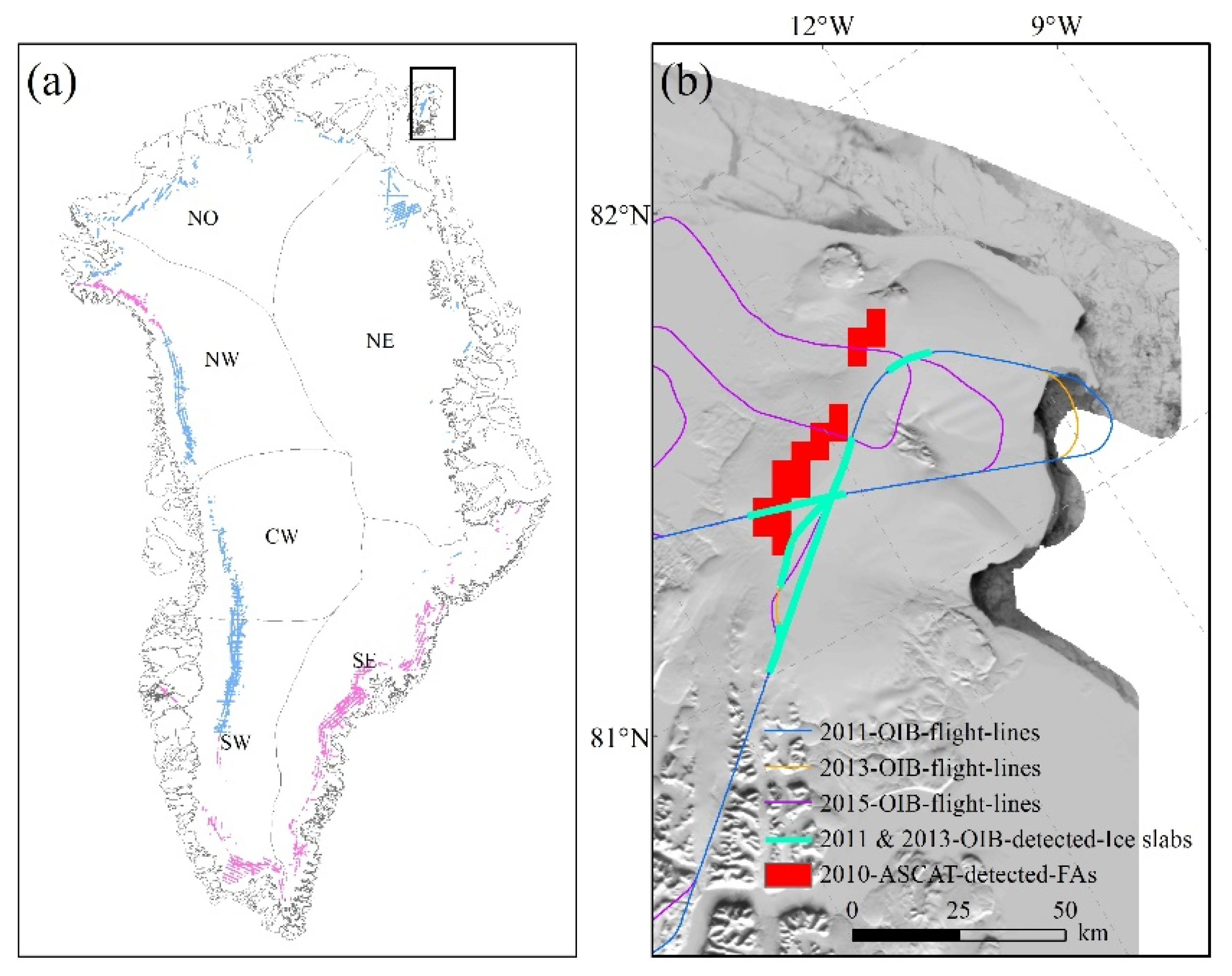
2.1. Data

2.1.1. Enhanced-Resolution Radar Scatterometer Data

The ASCAT instruments carried on the EUMETSAT Metop-A, Metop-B, and Metop-C satellites were launched in October 2006, September 2012, and November 2018 respectively, and are the following for Earth remote sensing satellite (ERS-1 and ERS-2) scatterometers [35,36]. The fan-beam ASCAT scatterometer measures radar backscatter in vertical polarization and has a diversity of incidence angles ranging from 25° to 65° at a frequency of 5.255 GHz (C-band). It has a wide swath and frequent overflights, permitting to generate radar backscatter images in the polar area rapidly.

We use the enhanced-resolution radar Scatterometer Image Reconstruction (SIR) product of ASCAT (2007–2020) from the NASA Scatterometer Climate Record Pathfinder (SCP) Project (http://www.scp.byu.edu, accessed on 11 June 2021). The SIR product is created from ASCAT L1B SZF files using the multi-variate SIR algorithm with filtering (SIRF) [37]. The SIR algorithm is a method for reconstructing images from raw scatterometer or radiometer data, based on a multivariate form of block multiplicative algebraic reconstruction [38]. It generates enhanced resolution gridded images from the irregularly spaced measurements based on a variable aperture function [39]. We use the ‘A’ image in the ASCAT SIR product, which is sigma-0 in dB normalized to 40 deg incidence angle (Figure 1). The product in Greenland compromises temporal and spatial resolutions and typically spans a 24-hr period, with a 2-day temporal resolution. The nominal image pixel resolution is 4.45 km, and the effective image resolution varies depending on region and sampling condition but is estimated to be 15 to 20 km [37].

2.1.2. OIB Airborne Radar Observation

To fill the gap of measurements between the ICESat-1 and ICESat-2 missions, NASA implemented the OIB Program to acquire airborne remote sensing observations in the areas undergoing rapid changes. The multifrequency radar instrumentation package, including Multichannel Coherent Radar Depth Sounder/Imager (MCoRDS/I), Accumulation Radar, Ku-Band Radar, and Snow Radar, designed and operated by the Center for Remote Sensing of Ice Sheets (CReSIS), has been aboard NASA airborne platforms since 2009 as a part of the OIB program and measures ice surface topography, near-surface internal layers, bedrock topography and snow thickness over sea ice [42,43]. The locations of FAs over the GrIS are derived from the Accumulation Radar data and MCoRDS/I data of the OIB program [29,31]. The Accumulation Radar is a wideband ultrahigh-frequency radar with a central wavelength of 750 MHz and bandwidth of 320 MHz (2010–2014,2017). It measures the internal layering and shallow ice thickness with a vertical resolution of 65 cm in snow or firn [42]. The central wavelength and the bandwidth of the MCoRDS/I are 195 MHz and 30 MHz (2010–2014,2017), 315 MHz and 270 MHz (2015), 300 MHz and 300 MHz (2016) [33]. The MCoRDS/I can measure the deep internal layering of the ice sheet and the ice-bedrock interface [42].

The liquid water contained in firn may increase the dielectric constant of the medium and slow electromagnetic wave propagation. High-reflectivity and high-amplitude return signals appear in the Accumulation Radar data if liquid water exists in internal snow layers due to the significant difference in dielectric constant value between the saturated firn and dry firn. For the MCoRDS/I data, the englacial liquid water may absorb radar signals, resulting in missing ice-bedrock interface echoes [42]. The different performances of the same identified FAs between the Accumulation Radar and the MCoRDS/I are shown in Figure 2 [44,45]. Miège et al. [29] and Brangers et al. [31] obtained the FAs locations in the GrIS by picking the bright reflection horizons in the radar echo strength profiles from the Accumulation Radar data (2010–2014, 2017) [31]. Due to the absence of Accumulation Radar data in 2015–2016, they obtained the FAs locations by identifying the missing bed echoes in the MCoRDS/I data [31].

The dataset used in this study includes 500,565 FAs points of coordinates identified from the OIB airborne radar flight lines, as shown in Figure 1 [40]. These FAs are distributed in 3308 ASCAT grids of the GrIS (

Table 1. Sample numbers of FAs and NFAs along the OIB flight lines.

	Number of Grids
Year	FAs	NFAs	Total
2010	252	4765	5017
2011	412	10,687	11,099
2012	491	12,309	12,800
2013	188	8698	8886
2014	291	8756	9047
2015	785	10,494	11,279
2016	463	5011	5474
2017	426	12,656	13,082
Total	3308	73,376	76,684

). NFAs represent the ASCAT grids with airborne radar flight lines passed but no FAs detection. We obtained the distribution of NFAs from annual airborne radar flight lines, with a total of 73,376 grids. According to the assumptions of Miller et al. [33], the effective grid cell size of the Accumulation Radar and MCoRDS/I points are 15 m × 20 m and 14 m × 40 m under the smooth surface. The uncertainty caused by the differences in the airborne radar detection area and ASCAT grid will be discussed in Section 4.1. The OIB-detected dataset also contains the FAs polygons interpolated by the OIB airborne radar flight lines according to the rules in Miège et al. [29]. The total combined FAs polygons extent in this dataset from 2010 to 2017 is 29,268 km², around the southeast, south, and northwest of the GrIS.

2.2. Methods

In this study, we first derive the melt days (MD), melt intensity (MI), and winter mean backscatter (WM) values of the grids along the OIB flight lines from the ASCAT data. According to the OIB-detected FAs dataset [40], we label these grids as FAs and NFAs grids (Table 1). Then the ASCAT-derived MD, MI, and WM values of these grids are input into the RF classification algorithm as the input vectors to train the model. Finally, we apply this model to classify all grids in the GrIS from 2010 to 2020. In Section 2.2.1 and Section 2.2.2, we introduce the ASCAT-derived parameters and the RF classification method.

2.2.1. Selection of Input Vectors

During the melting season, meltwater fills the firn pores above a certain depth of firn, below which the ice temperature would freeze liquid water [18]. As the snow accumulates, the snow layer insulates the aquifers from refreezing and the FAs may still exist as liquid form throughout winter. Therefore, the formation and recharge of FAs are related to the amount of surface snowmelt produced during the melt season and the snow accumulation during the autumn to next early spring [14,31]. Based on the previous studies, we obtained three parameters from ASCAT data to represent surface snowmelt and snow accumulation of the GrIS.

Liquid water presented in snow or firn is a result of surface snowmelt, resulting in a higher dielectric constant and an increase in microwave absorption and leading to a large decrease in backscattering coefficient (${\sigma }^0$) compared with dry snow [46,47,48]. Radar scatterometers are widely utilized in the detection of surface snowmelt in Greenland and the Antarctic [49,50,51,52,53,54]. MD is always used to describe the surface melt conditions [46,47,48,49,51]. Zheng et al. [51] found that liquid water intensity (LWI), also named melt intensity (MI) [55], and melting decibel-days (MDD) [47] generated by satellites have high correlations with the RACMO2 liquid water volume. Therefore, we choose the MD and MI parameters to evaluate surface melt conditions which may influence the formation of the FAs. Through testing experiments, MD and MI parameters can be used simultaneously to achieve higher classification accuracy.

Surface snowmelt (M) is determined when the ${\sigma }^0$ falls below a constant threshold for the WM (Equation (1)) [46,47,48,51]. MD is commonly used for surface snowmelt detection in Greenland and Antarctica [55,56,57] and is calculated by summing up the days when surface snowmelt is present throughout the year with a constant threshold algorithm (CTA) in Equation (2). MI is calculated by summing the difference between the WM and ${\sigma }_i^0$ on melt days throughout the whole year for each pixel as per Equation (3).

$$M\left(i\right)=\{\begin{array}{c} 0,if {\sigma }_i^0>{\sigma }_{\mathrm{wm}}^0-b \\ 1,if {\sigma }_i^0\le {\sigma }_{\mathrm{wm}}^0-b\end{array}$$

(1)

$$\mathrm{MD}={{\displaystyle \sum }}_{i=June 1,year}^{i=May 31,year+1}M\left(i\right)$$

(2)

$$\mathrm{MI}={{\displaystyle \sum }}_{i=June 1,year}^{i=May 31,year+1}M\left(i\right)({\sigma }_{\mathrm{wm}}^0-{\sigma }_i^0)$$

(3)

where ${\sigma }_i^0$ is the pixel daily backscatter in dB normalized to 40 deg incidence angle, and ${\sigma }_{wm}^0$ is the pixel WM (December to February). For the ASCAT scatterometer instruments, according to Ashcraft and Long [46], the constant threshold b is set to 2.7 dB, which does not vary spatially and temporally. It is assumed that the formation of FAs is associated with the meltwater in melt season (June to August). Therefore, we designed the calculation of MD and MI starting from 1 June to 31 May in the following year to capture the melting season (June to August) and freezing season (December to February).

Several microwave measurements have been used to estimate snow accumulation in the percolation zone and dry-snow zone of the GrIS [58,59,60,61]. According to Wismann et al. [58], the dry-snow accumulation on the firn of the percolation zone may decrease the backscatter of ERS-1 and ERS-2 scatterometers. They derived the thickness of dry snow overlying the percolation zone and snow accumulation rate by a two-layer radar backscatter model. Nghiem et al. [61] also found that the linear decrease in backscatter measurements of the QuikSCAT scatterometer during the freezing season is related to the amount of snow accumulation over the ice layer formation region in the percolation zone. Because of the two-way attenuation in the dry snow, the backscatter contribution of large scatterers in the firn layer created by melt metamorphosis becomes weaker. Based on the above research, we speculate that the difference in backscatter value in different years can reflect the change of accumulation rate and the winter mean backscatter (WM) value can reflect the accumulation conditions during the freezing season.

Through the above method, we obtain the ASCAT-derived MD, MI, and WM results from 2007 to 2020 for each pixel (Figure 3). The time-line interpolation method is used to interpolate the missing ASCAT observation data [51].

2.2.2. Random Forests Classification Algorithm

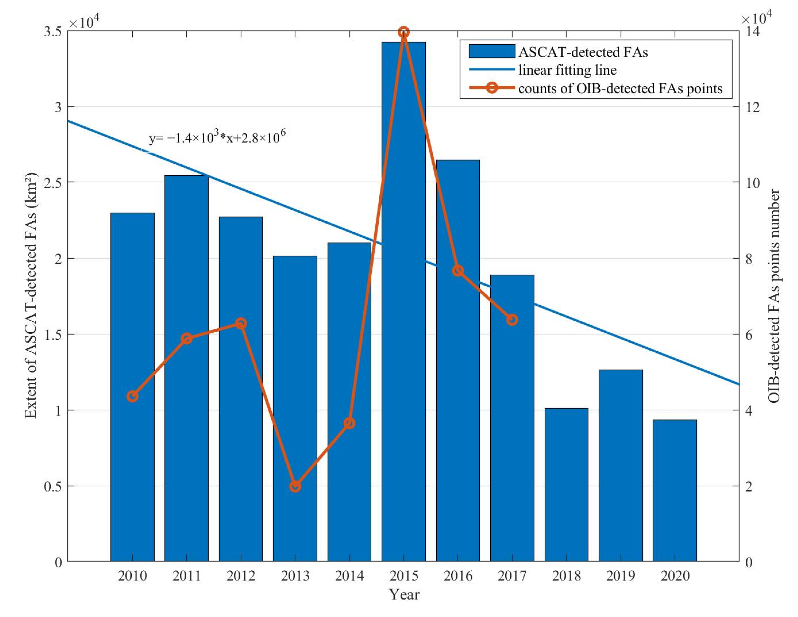
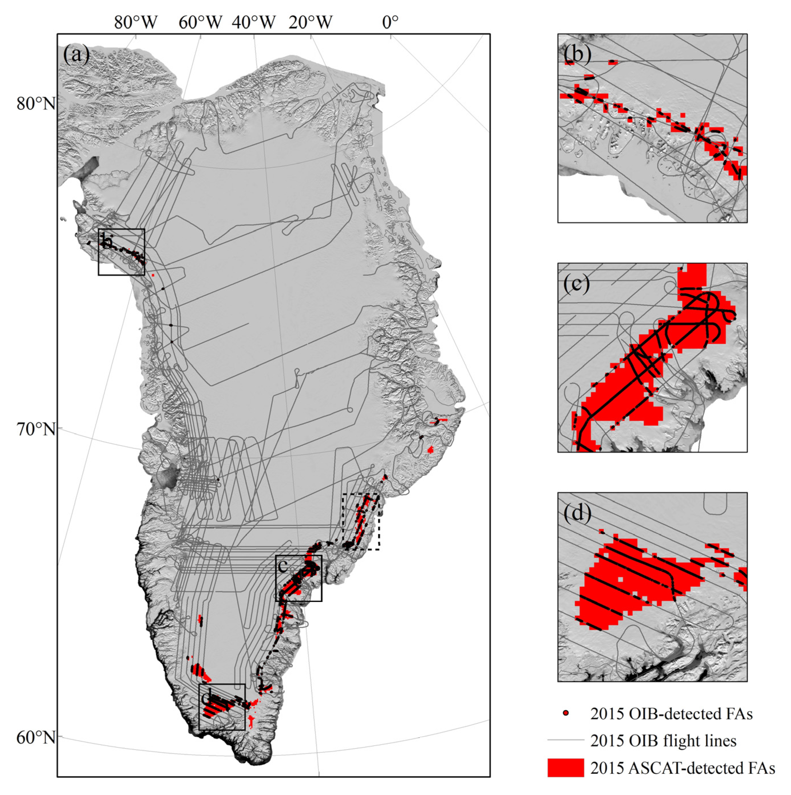
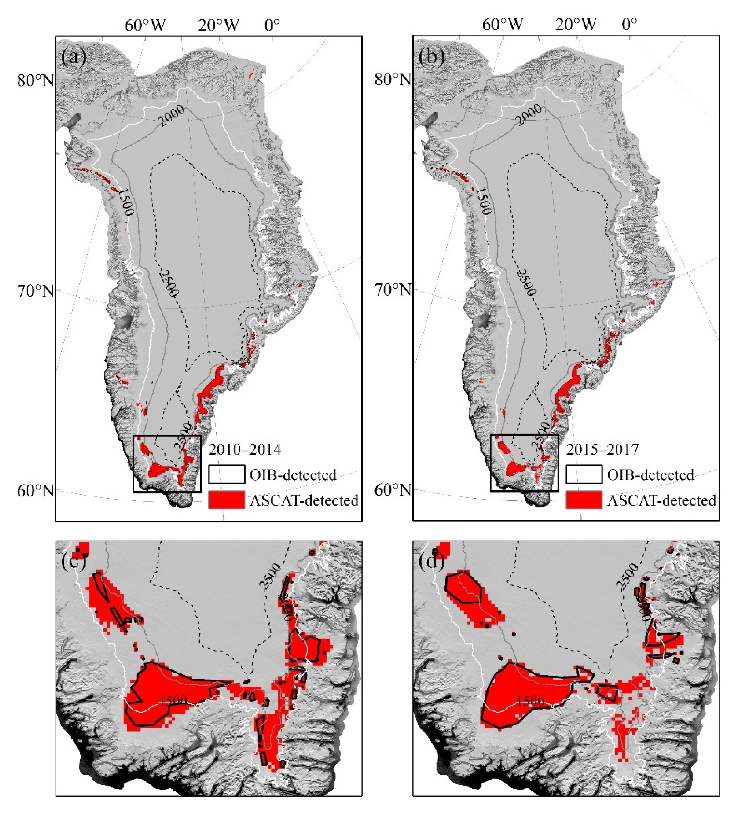
Considering the complexity of snow accumulation and melting conditions in the GrIS, we choose the machine learning algorithm to distinguish FAs and NFAs grids instead of the simple threshold algorithm. Compared with other machine learning algorithms, the Random Forests (RF) algorithm needs fewer parameter adjustments and has the advantages of having a fast training speed, short processing time, strong generalization ability, and great performance on many remote sensing data sets [63,64]. After being developed by Breiman [65], the RF algorithm has been widely used in remote sensing applications, such as vegetation cover classification, geological mapping, etc. [64,66,67,68,69,70]. The RF, a simple and efficient machine learning algorithm, uses multiple decision trees to train, classify and predict the samples. Each decision tree votes the result depending on the value of an independently sampled random vector. The RF algorithm assumes that there are N samples in the training set, each sample has D features, and the forest containing T trees needs to be trained. Each decision tree in the RF algorithm follows the next operation. Firstly, a sub-training set of size N is obtained from the training set by sampling with placement. Then, M features (M ≤ D) which represent the number of random variables available at each node are randomly selected from D features. Finally, each tree gets its own classification rules by training sub-training sets. The final category for the classification is determined according to the voting results in the forest. In the sampling with replacement, some samples may appear multiple times in the same sub-training set, and some samples may be ignored. In each sample, the probability of each one being picked is $\frac{1}{N}$, so the probability of not being picked is $1-\frac{1}{N}$, and the probability of not being drawn in N samples is ${\left(1-\frac{1}{N}\right)}^N$ going to converge to $\frac{1}{e}$, which is about 0.37. Therefore, if the dataset is large enough, about 37% of the training data will not participate in the training, which is called out of bag (OOB) data. Through assessing the classification accuracy of OOB data, we can obtain the inner cross-validation result of RF, which is called out-of-bag error (OOBE).

According to the model simulation and airborne radar measurements, the FAs in some areas can last for many years [16,29]. We assume the existence of FAs is also closely related to the surface snowmelt and snow accumulation in previous years. Therefore, we also put the MD, MI, and WM parameters in previous melt cycles of the FAs and NFAs grids into the RF classification algorithm. For example, the ‘1-year’ model in

Table 2. Accuracy of models with different input vectors.

Model	Kappa	OA(%)	TN	TP	FN	FP
1-year	0.56	96.20	3638	103	94	54
2-year	0.68	97.15	3652	126	71	40
3-year	0.72	97.49	3657	134	63	35
4-year	0.72	97.57	3659	135	62	33
5-year	0.73	97.60	3659	136	60	33
6-year	0.74	97.63	3659	137	59	33
7-year *	0.74	97.47	3659	138	59	33

* The ‘7-year’ model indicates that the MD, MI, and WM parameters within seven melt cycles of each trained grid are included as input vectors integrated into the model.

indicates that the MD, MI, and WM parameters within one year of the grids in which airborne radar flight lines pass are put into the algorithm. We compare the classification results with different models and assessed the classification accuracy of different models by using the ten-fold cross-validation method for the training data from 2014 to 2017 (Table 2). In this test, the number of decision trees (T) was 200, and the default value was set to the random variables (M). The overall accuracy (OA), Kappa coefficient, and confusion matrix (TN, TP, FN, FP) were used as classifier performance metrics to measure the performance of different models in Equations (4)–(6). From the OA and Kappa coefficient presented in Table 2, we found that the more input vectors integrated into the model, the higher the classification accuracy. After the model was integrated with the ‘3-year’ of input vectors, the improvement of classification accuracy become slow. As ASCAT data started from 2007 and OIB-detected FAs started from 2010, when the model was more than ‘3-years’, the number of grids available for training is gradually decreasing. To obtain training grids and classification results of more years, we finally chose the ‘3-year’ model for training and classification.

$$OA=\frac{TP+TN}{TP+TN+FP+FN}$$

(4)

$$P_e=\frac{\left(TP+FN\right)\times \left(TP+FP\right)+\left(FN+TN\right)\times \left(TN+FP\right)}{N^2}$$

(5)

$$Kappa=\frac{OA-P_e}{1-P_e}$$

(6)

The RF algorithm is easy to optimize because it has only T and M two parameters to adjust. By calculating the OOBE with different T for the training data from 2010 to 2017 under the ‘3-year’ model, we found that the OOBE decreased with the increase of T, and remained stable when the T was above a certain value. Figure 4a shows that when the T is under 50, OOBE decreases rapidly; when the T is within 50–200, OOBE shows very little change; when the T is greater than 200, OOBE is considered to be stable. Therefore, T is set to 200 as a tradeoff between maintaining high accuracy and reducing calculation costs. Previous experiments show that the number of M set on each node has little effect on the classification accuracy [70]. The MD, MI, and WM parameters in three melt cycles were taken as input vectors under the ‘3-year’ model, with a total of nine variables. We tested M from 1 to 9 to determine the number of predictor variables based on the method presented by Breiman [65]. In Figure 4b, we find that the M variable has little effect on the OOBE results. Finally, we used 200 trees and default M to train the data from 2010 to 2017 under the ‘3-year’ model. The RF classification discussed above is implemented under the Matlab environment (R2019a).

3. Results

Based on the ‘3-year’ model RF classifier described in Section 2.2.2, we obtain the FAs locations of each year from 2010 to 2020 (Figure 5). The accumulative FAs area from 2010 to 2020 (which means the repeated FAs grids between 2010 and 2020 are counted only once) is 56,477 km², which is 3.3% of the GrIS area. Approximately 88.4% of FAs are distributed at altitudes less than 2000 m, while 11.6% are located between 2000 m to 2500 m. From the result of 2010 to 2020 (Figure 6), 90% of FAs are distributed in the SW and SE basins of the GrIS and only 8% in the NW basins [41]. FAs are also found on three ice caps in the northeast and southwest, but largely absent in the NO, CW, and NE basins of the GrIS. FAs are relatively stable in the south and southeast, while FAs are scattered and unstable in the central west and central east.

Inter-annual analysis suggests the annual ASCAT-detected FAs area is relatively stable between 2010 and 2014, reaching the maximum area of 34,219 km² in 2015 (Figure 7 and

Table 3. Statistical results of FAs area in different periods.

Year	OIB-Detected	ASCAT-Detected
	Area/km2	Area/km2
2010	-	22,971
2011	-	25,446
2012	-	22,713
2013	-	20,139
2014	-	20,991
2015	-	34,219
2016	-	26,476
2017	-	18,872
2018	-	10,079
2019	-	12,634
2020	-	9347
2010–2020	-	56,477
2010–2014	22,947	45,526
2015–2017	22,858	42,179

). The areas of FAs show a gradual decline from 2015 to 2020, reaching the minimum area of 9347 km² in 2020. Similar inter-annual variations are found within the FAs points detected by OIB airborne radar over the flight lines (Figure 7). According to the linear fitting result of the extent of the ASCAT-detected and year, the area of FAs tends to decrease.

According to the enlarged Figures of the results in 2015 (Figure 8b–d), the detection of FAs in the northwest, southeast, and south of the GrIS is in good agreement with the FAs detected by OIB. The distance between the two parallel OIB flight lines in Figure 8c,d is about 20 km, which is bigger than the grid size of ASCAT SIR products.

Miege et al. [29] and Brangers et al. [31] interpolated the extent of aquifers between OIB flight lines from 2010 to 2014 and 2015 to 2017. We compare the results of the two methods during 2010–2014 and 2015–2017 and find that ASCAT-detected FAs cover the polygons extracted from the airborne radar data (Figure 9 and Table 3). The ASCAT-detected accumulative FAs areas during 2010–2014 and 2015–2017 are 98% and 85% higher than that from the OIB polygons. We analyze the evolution of FAs in the southern GrIS region from 2010 to 2020 and find that the temporal and spatial changes of FAs are significant during this period (Figure 10).

4. Discussion

4.1. Comparisons and Uncertainties

Satellite observations provide a way to continuously monitor FAs over the GrIS. In Figure 9 and Table 3, we compare our ASCAT-detected results with the OIB-detected FAs polygons interpolated by the OIB flight lines over the same period. The ASCAT-detected accumulative FAs areas are 98% and 85% higher than the OIB-detected FAs polygons [29,31]. This is because the OIB-detected results only cover areas crossed by OIB airborne radar flight lines, excluding areas that may contain FAs but are not crossed by flight lines. The extent of OIB-detected FAs may be underestimated due to the limitations in spatial and temporal resolution. The FAs monitored by satellite remote sensing have the advantage of a wider detection range. The FAs extent detected by Sentinel-1 of Brangers et al. [31] was 54,800 km² in 2014–2019, similar to the accumulative ASCAT-detected FAs area of 56,477 km² from 2010 to 2020 in our study. The difference between the two ways may result from two aspects: on the one hand, the FAs mosaic obtained by Sentinel-1 may include the areas where liquid water exists in September but freezes in winter; on the other hand, the ice lens above the aquifer and surface melt production in September may also affect the detection of FAs in the Sentinel-1 algorithm [31]. In this study, the uncertainties of our results are from the following aspects.

The FAs and NFAs grids trained in the RF classification algorithm are labeled by the OIB-detected FAs dataset [40]. The uncertainties in the OIB-detected FAs dataset may affect the accuracy of ASCAT-detected FAs. According to the research of Miege et al. [29], the uncertainties of the OIB-detected FAs dataset reflect in three aspects [29]. Firstly, the quality of OIB radar data heavily relies on the flight status of aircraft such as turbulence and turning geometry. Secondly, the Accumulation Radar cannot detect the FAs with a depth of more than 40 m because of the weak returns from internal layers which are masked by the surface clutter. Lastly, a combination of semi-automatic and manual identification methods in the detection of the FAs over the OIB flight lines may result in some artificial biases, especially at the edge of the aquifers where the radar signal is weak.

The effective resolution of airborne radar detection data may also affect the FAs detections. As per the research of Miller et al. [33], the effective grid cell size of the Accumulation Radar (15 m × 20 m) and MCoRDS/I (14 m × 40 m) points are much smaller than the effective resolution of the ASCAT data. In our study, grids with airborne radar flight lines but no OIB-detected FAs are labeled as NFAs, but this does not mean that firn aquifers are not present at other locations of these ASCAT grids. For this reason, our results may be smaller than the true conditions.

When the volume fraction of liquid water in the snow and firn layers is high, the penetration depth of ASCAT may be only tens of centimeters in wet snow [54,72]. Since the penetration depth of the ASCAT signal cannot reach the depth of FAs, we did not use the backscatter information of ASCAT to directly indicate the existence of FAs. Instead, the MD, MI, and WM parameters derived from the backscatter value were used to characterize the surface snowmelt and the snow accumulation in our study. To obtain the snowmelt of the GrIS, we utilized the CTA algorithm, with the constant threshold b set as 2.7 dB as described in Section 2.2.1. However, the study showed that the snow properties, such as snow depth, density, and grain size, may influence the response of radar backscatter to snowmelt, leading to temporal variations in ${\sigma }^0$ time-series [73]. Therefore, using a single threshold to identify snowmelt may produce misclassification errors. At the same time, the ASCAT instrument can penetrate tens of meters in dry snow, so the melting signal detected may not only be surface snowmelt but could also include subsurface melt or liquid water remaining after surface refreeze [46].

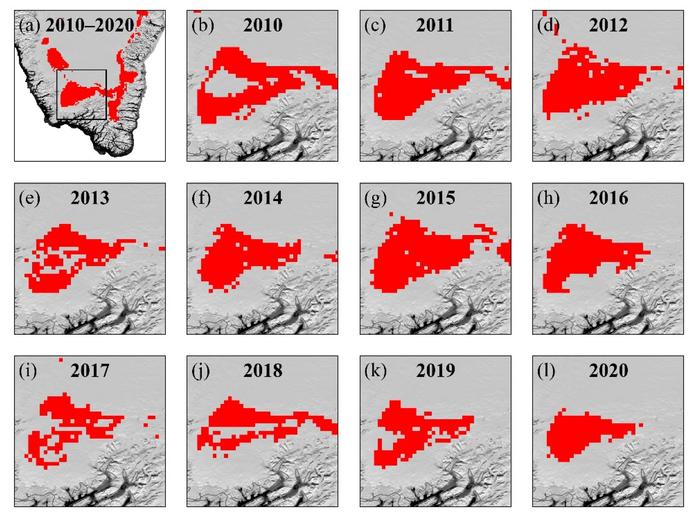
4.2. FAs in the Flade Isblink Ice Cap

FAs are found in the Flade Isblink ice cap of the northeast GrIS according to our ASCAT-detected results in 2010 but have not been reported in previous studies. We found that no OIB airborne radars flight lines covered this area in 2010. In 2011, 2013, and 2015, the OIB aircraft flew over the adjacent area, FAs were not detected from the Accumulation Radar data (2011, 2013) and the MCoRDS/I data (2015). But in 2011 and 2013, the ice slabs were detected from Accumulation Radar (Figure 11) [74]. FAs and ice slabs are the two main components of the percolation zone in the GrIS [33]. We speculate that the formation of ice slabs in 2011 is related to the FAs in 2010. No FAs are detected in this region in our study from 2011 to 2020, maybe because of the formation of low-permeability ice slabs. According to Figure 11a, the FAs and ice slabs do not overlap each other and are located in different regions of the GrIS.

4.3. FAs Anomalies in the Eastern of the GrIS

By comparing the differences between each year, we find that FAs are more widespread in 2015 in the eastern GrIS (the black dashed box in Figure 8). According to the ASCAT-detected result, the King Christian IX Land experienced widespread FAs in 2015, which was not common in other years. By analyzing the MD, MI, and WM parameters of the ASCAT-detected FAs in this region, we found that WM is significantly different from the multi-year average. In this study, we derived the WM from the ASCAT data to represent the snow accumulation. To calculate the annual snow accumulation at the ASCAT-detected FAs in this region from 2009 to 2020, we downloaded the snowfall and snow evaporation variables from the ERA5 monthly averaged dataset of the extent in the black dashed box in Figure 8 [75]. The annual snow accumulation is calculated by summing up the monthly snow accumulation which is the difference between snowfall and evaporation/sublimation [76]. The results show that the snow accumulation from 1 June 2014 to 31 May 2015 was 2080 mmWE (mm of water equivalent), which was 382 mmWE higher than the average of 1698 mmWE from 2009 to 2020 and 619 mmWE higher than the average of 1461 mmWE from 2009 to 2014. We hypothesize that the widespread FAs detected in King Christian IX Land in 2015 are related to snow accumulation anomalies.

The ASCAT-detected FAs locations are consistent with some previous snow/firn models studies, in which liquid water content is reported to be mainly distributed in the northwestern, southern, and southeastern regions of the GrIS [17,77]. According to the RACMO2 simulations, these areas have high accumulation (>800 mm yr⁻¹) and large liquid water production (snowmelt plus rain > 650 mm yr⁻¹), which are the necessary conditions for FAs formation [14]. In the future, we will study the relations of the parameters which play a key role in the formation of FAs between remote sensing data and regional climate models.

5. Conclusions

In this study, the inter-annual variations of FAs over the GrIS are investigated based on the enhanced-resolution ASCAT observations by the RF classification algorithm with the aid of the OIB-detected FAs locations. The ASCAT-derived MD, MI, and WM are the input vectors of the FAs retrieval model. We obtained the extent of the FAs in each year from 2010 to 2020. The accumulative FAs area from 2010 to 2020 is 56,477 km², which is 3.3% of the GrIS area. The locations of FAs extracted by the RF algorithm agreed well with the detection results of airborne radar. ASCAT-detected accumulative FAs areas are 98% and 85% higher than the OIB polygons during the periods of 2010–2014 and 2015–2017, respectively. The ASCAT data has a wider space coverage and better time continuity than the OIB airborne radar data, enabling us to detect the whole GrIS and analyze the dynamic change in FAs.

Through continuous FAs monitoring for a decade, we found that the FAs change dynamically depending on the surface melt and accumulation conditions. As global temperatures continue to rise, the percolation zone of the GrIS may gradually expand inland, and the cover of the FAs may gradually expand to a higher elevation which was proved in Helheim Glacier [18]. Long-term time series scatterometer data records enable us to better understand the distribution and formation mechanism of FAs which help us to predict the future changes in the GrIS and their impact on global sea-level rise.

References

1. Zwally, H.J.; Abdalati, W.; Herring, T.; Larson, K.; Saba, J.; Steffen, K. Surface Melt-Induced Acceleration of Greenland Ice-Sheet Flow. Science 2002, 297, 218–222. [Google Scholar] [CrossRef] [PubMed]
2. Dowdeswell, J.A. The Greenland Ice Sheet and Global Sea-Level Rise. Science 2006, 311, 963–964. [Google Scholar] [CrossRef] [PubMed]
3. Hanna, E.; Navarro, F.J.; Pattyn, F.; Domingues, C.M.; Fettweis, X.; Ivins, E.R.; Nicholls, R.J.; Ritz, C.; Smith, B.; Tulaczyk, S.; et al. Ice-sheet mass balance and climate change. Nature 2013, 498, 51–59. [Google Scholar] [CrossRef]
4. Van den Broeke, M.; Bamber, J.; Ettema, J.; Rignot, E.; Schrama, E.; van de Berg, W.J.; van Meijgaard, E.; Velicogna, I.; Wouters, B. Partitioning Recent Greenland Mass Loss. Science 2009, 326, 984–986. [Google Scholar] [CrossRef] [PubMed] [Green Version]
5. van de Wal, R.S.W.; Boot, W.; van de Broeke, M.R.; Smeets, C.J.P.P.; Reijmer, C.H.; Donker, J.J.A.; Oerlemans, J. Large and Rapid Melt-Induced Velocity Changes in the Ablation Zone of the Greenland Ice Sheet. Science 2008, 321, 111–113. [Google Scholar] [CrossRef] [PubMed]
6. Shannon, S.R.; Payne, A.J.; Bartholomew, I.D.; van de Broeke, M.R.; Edwards, T.L.; Fettweis, X.; Gagliardini, O.; Gillet-Chaulet, F.; Goelzer, H.; Hoffman, M.J.; et al. Enhanced basal lubrication and the contribution of the Greenland ice sheet to future sea-level rise. Proc. Natl. Acad. Sci. USA 2013, 110, 14156–14161. [Google Scholar] [CrossRef] [Green Version]
7. Schoof, C. Ice-sheet acceleration driven by melt supply variability. Nature 2010, 468, 803–806. [Google Scholar] [CrossRef]
8. Sundal, A.V.; Shepherd, A.; Nienow, P.; Hanna, E.; Palmer, S.; Huybrechts, P. Melt-induced speed-up of Greenland ice sheet offset by efficient subglacial drainage. Nature 2011, 469, 521–524. [Google Scholar] [CrossRef]
9. van de Broeke, M.R.; Enderlin, E.M.; Howat, I.M.; Munneke, P.K.; Noël, B.P.Y.; van de Berg, W.J.; van Meijgaard, E.; Wouters, B. On the recent contribution of the Greenland ice sheet to sea level change. Cryosphere 2016, 10, 1933–1946. [Google Scholar] [CrossRef] [Green Version]
10. Andrew, S.; Erik, I.; Eric, R.; Ben, S.; van den Broeke, M.; Isabella, V.; Pippa, W.; Kate, B.; Ian, J.; Gerhard, K.; et al. Mass balance of the Greenland Ice Sheet from 1992 to 2018. Nature 2020, 579, 233–239. [Google Scholar] [CrossRef]
11. Dunmire, D.; Banwell, A.F.; Wever, N.; Lenaerts, J.T.M.; Datta, R.T. Contrasting regional variability of buried meltwater extent over 2 years across the Greenland Ice Sheet. Cryosphere 2021, 15, 2983–3005. [Google Scholar] [CrossRef]
12. Houtz, D.; Mätzler, C.; Naderpour, R.; Schwank, M.; Steffen, K. Quantifying Surface Melt and Liquid Water on the Greenland Ice Sheet using L-band Radiometry. Remote Sens. Environ. 2021, 256, 112341. [Google Scholar] [CrossRef]
13. Pitcher, L.H.; Smith, L.C.; Gleason, C.J.; Miège, C.; Ryan, J.C.; Hagedorn, B.; van As, D.; Chu, W.; Forster, R.R. Direct Observation of Winter Meltwater Drainage from the Greenland Ice Sheet. Geophys. Res. Lett. 2020, 47, e2019GL086521. [Google Scholar] [CrossRef] [Green Version]
14. Forster, R.R.; Box, J.E.; Van Den Broeke, M.R.; Miège, C.; Burgess, E.W.; Van Angelen, J.H.; Lenaerts, J.T.M.; Koenig, L.S.; Paden, J.; Lewis, C.; et al. Extensive liquid meltwater storage in firn within the Greenland ice sheet. Nat. Geosci. 2014, 7, 95–98. [Google Scholar] [CrossRef]
15. Montgomery, L.; Miège, C.; Miller, J.; Scambos, T.A.; Wallin, B.; Miller, O.; Solomon, D.K.; Forster, R.; Koenig, L. Hydrologic Properties of a Highly Permeable Firn Aquifer in the Wilkins Ice Shelf, Antarctica. Geophys. Res. Lett. 2020, 47, e2020GL089552. [Google Scholar] [CrossRef]
16. van Wessem, J.M.; Steger, C.R.; Wever, N.; Van Den Broeke, M.R. An exploratory modelling study of perennial firn aquifers in the Antarctic Peninsula for the period 1979–2016. Cryosphere 2021, 15, 695–714. [Google Scholar] [CrossRef]
17. Munneke, P.K.; Ligtenberg, S.R.M.; Van Den Broeke, M.R.; van Angelen, J.H.; Forster, R.R. Explaining the presence of perennial liquid water bodies in the firn of the Greenland Ice Sheet. Geophys. Res. Lett. 2014, 41, 476–483. [Google Scholar] [CrossRef] [Green Version]
18. Miller, O.; Solomon, D.K.; Miège, C.; Koenig, L.; Forster, R.; Schmerr, N.; Ligtenberg, S.R.M.; Legchenko, A.; Voss, C.I.; Montgomery, L.; et al. Hydrology of a Perennial Firn Aquifer in Southeast Greenland: An Overview Driven by Field Data. Water Resour. Res. 2020, 56, e2019WR026348. [Google Scholar] [CrossRef]
19. Harper, J.; Humphrey, N.; Pfeffer, W.T.; Brown, J.; Fettweis, X. Greenland ice-sheet contribution to sea-level rise buffered by meltwater storage in firn. Nature 2012, 491, 240–243. [Google Scholar] [CrossRef]
20. Nienow, P.W.; Sole, A.J.; Slater, D.A.; Cowton, T.R. Recent Advances in Our Understanding of the Role of Meltwater in the Greenland Ice Sheet System. Curr. Clim. Chang. Rep. 2017, 3, 330–344. [Google Scholar] [CrossRef] [Green Version]
21. Poinar, K.; Joughin, I.; Lilien, D.; Brucker, L.; Kehrl, L.; Nowicki, S. Drainage of Southeast Greenland Firn Aquifer Water through Crevasses to the Bed. Front. Earth Sci. 2017, 5, 5. [Google Scholar] [CrossRef] [Green Version]
22. Koenig, L.S.; Miège, C.; Forster, R.R.; Brucker, L. Initial in situ measurements of perennial meltwater storage in the Greenland firn aquifer. Geophys. Res. Lett. 2014, 41, 81–85. [Google Scholar] [CrossRef] [Green Version]
23. Christianson, K.; Kohler, J.; Alley, R.B.; Nuth, C.; van Pelt, W.J.J. Dynamic perennial firn aquifer on an Arctic glacier. Geophys. Res. Lett. 2015, 42, 1418–1426. [Google Scholar] [CrossRef]
24. Machguth, H.; MacFerrin, M.; van As, D.; Box, J.E.; Charalampidis, C.; Colgan, W.; Fausto, R.S.; Meijer, H.A.J.; Mosley-Thompson, E.; Van De Wal, R.S.W. Greenland meltwater storage in firn limited by near-surface ice formation. Nat. Clim. Chang. 2016, 6, 390–393. [Google Scholar] [CrossRef] [Green Version]
25. Miller, O.; Solomon, D.K.; Miège, C.; Koenig, L.; Forster, R.; Schmerr, N.; Ligtenberg, S.R.M.; Montgomery, L. Direct Evidence of Meltwater Flow within a Firn Aquifer in Southeast Greenland. Geophys. Res. Lett. 2018, 45, 207–215. [Google Scholar] [CrossRef] [Green Version]
26. Killingbeck, S.F.; Schmerr, N.C.; Montgomery, L.N.; Booth, A.D.; Livermore, P.W.; Guandique, J.; Miller, O.L.; Burdick, S.; Forster, R.R.; Koenig, L.S.; et al. Integrated Borehole, Radar, and Seismic Velocity Analysis Reveals Dynamic Spatial Variations within a Firn Aquifer in Southeast Greenland. Geophys. Res. Lett. 2020, 47, e2020GL089335. [Google Scholar] [CrossRef]
27. Montgomery, L.N.; Schmerr, N.; Burdick, S.; Forster, R.R.; Koenig, L.; Legchenko, A.; Ligtenberg, S.; Miège, C.; Miller, O.L.; Solomon, D.K. Investigation of Firn Aquifer Structure in Southeastern Greenland Using Active Source Seismology. Front. Earth Sci. 2017, 5, 10. [Google Scholar] [CrossRef] [Green Version]
28. Killingbeck, S.; Schmerr, N.; Montgomery, L.; Booth, A.; Livermore, P.; Guandique, J.; Miller, O.; Burdick, S.; Forster, R.; Koenig, L.; et al. Deriving water content from multiple geophysical properties of a firn aquifer in southeast Greenland. In Proceedings of the EGU General Assembly 2020, Online, 4–8 May 2020. [Google Scholar] [CrossRef]
29. Miège, C.; Forster, R.R.; Brucker, L.; Koenig, L.S.; Solomon, D.K.; Paden, J.D.; Box, J.E.; Burgess, E.W.; Miller, J.Z.; McNerney, L.; et al. Spatial extent and temporal variability of Greenland firn aquifers detected by ground and airborne radars. J. Geophys. Res. Earth Surf. 2016, 121, 2381–2398. [Google Scholar] [CrossRef]
30. Chu, W.; Schroeder, D.M.; Siegfried, M.R. Retrieval of Englacial Firn Aquifer Thickness from Ice-Penetrating Radar Sounding in Southeastern Greenland. Geophys. Res. Lett. 2018, 45, 11,770–11,778. [Google Scholar] [CrossRef]
31. Brangers, I.; Lievens, H.; Miège, C.; Demuzere, M.; Brucker, L.; De Lannoy, G.J.M. Sentinel-1 Detects Firn Aquifers in the Greenland Ice Sheet. Geophys. Res. Lett. 2020, 47, e2019GL085192. [Google Scholar] [CrossRef] [Green Version]
32. Miller, J.Z.; Long, D.G.; Jezek, K.C.; Johnson, J.T.; Brodzik, M.J.; Shuman, C.A.; Koenig, L.S.; Scambos, T.A. Brief communication: Mapping Greenland’s perennial firn aquifers using enhanced-resolution L-band brightness temperature image time series. Cryosphere 2020, 14, 2809–2817. [Google Scholar] [CrossRef]
33. Miller, J.Z.; Culberg, R.; Long, D.G.; Shuman, C.A.; Schroeder, D.M.; Brodzik, M.J. An empirical algorithm to map perennial firn aquifers and ice slabs within the Greenland Ice Sheet using satellite L-band microwave radiometry. Cryosphere 2022, 16, 103–125. [Google Scholar] [CrossRef]
34. Samimi, S.; Marshall, S.J.; Vandecrux, B.; MacFerrin, M. Time-Domain Reflectometry Measurements and Modeling of Firn Meltwater Infiltration at DYE-2, Greenland. J. Geophys. Res. Earth Surf. 2021, 126, e2021JF006295. [Google Scholar] [CrossRef]
35. Figa-Saldaña, J.; Wilson, J.J.W.; Attema, E.; Gelsthorpe, R.; Drinkwater, M.R.; Stoffelen, A. The advanced scatterometer (ASCAT) on the meteorological operational (MetOp) platform: A follow on for European wind scatterometers. Can. J. Remote Sens. 2002, 28, 404–412. [Google Scholar] [CrossRef]
36. Long, D.G. Polar Applications of Spaceborne Scatterometers. IEEE J. Sel. Top. Appl. Earth Obs. Remote Sens. 2017, 10, 2307–2320. [Google Scholar] [CrossRef] [Green Version]
37. Lindsley, R.D.; Long, D.G. Enhanced-Resolution Reconstruction of ASCAT Backscatter Measurements. IEEE Trans. Geosci. Remote Sens. 2016, 54, 2589–2601. [Google Scholar] [CrossRef]
38. Long, D.G.; Hardin, P.J.; Whiting, P.T. Resolution enhancement of spaceborne scatterometer data. IEEE Trans. Geosci. Remote Sens. 1993, 31, 700–715. [Google Scholar] [CrossRef] [Green Version]
39. Early, D.S.; Long, D.G. Image reconstruction and enhanced resolution imaging from irregular samples. IEEE Trans. Geosci. Remote Sens. 2001, 39, 291–302. [Google Scholar] [CrossRef] [Green Version]
40. Miège, C. Spatial Extent of Greenland Firn Aquifer Detected by Airborne Radars, 2010–2017. Arctic Data Center. 2018. Available online: https://arcticdata.io/catalog/view/doi%3A10.18739%2FA2TM72225 (accessed on 20 June 2021).
41. Rignot, E.; Mouginot, J. Ice flow in Greenland for the International Polar Year 2008–2009. Geophys. Res. Lett. 2012, 39, 11. [Google Scholar] [CrossRef] [Green Version]
42. Rodriguez-Morales, F.; Gogineni, S.; Leuschen, C.J.; Paden, J.D.; Li, J.; Lewis, C.C.; Panzer, B.; Alvestegui, D.G.G.; Patel, A.; Byers, K.; et al. Advanced Multifrequency Radar Instrumentation for Polar Research. IEEE Trans. Geosci. Remote Sens. 2014, 52, 2824–2842. [Google Scholar] [CrossRef]
43. Lewis, C.; Gogineni, S.; Rodriguez-Morales, F.; Panzer, B.; Stumpf, T.; Paden, J.; Leuschen, C. Airborne fine-resolution UHF radar: An approach to the study of englacial reflections, firn compaction and ice attenuation rates. J. Glaciol. 2015, 61, 89–100. [Google Scholar] [CrossRef] [Green Version]
44. CReSIS. Accumulation Radar Data, Lawrence, KS, USA. Digital Media. 2021. Available online: https://data.cresis.ku.edu (accessed on 15 June 2021).
45. CReSIS. Radar Depth Sounder Data, Lawrence, KS, USA. Digital Media. 2021. Available online: https://data.cresis.ku.edu (accessed on 15 June 2021).
46. Ashcraft, I.S.; Long, D.G. Comparison of methods for melt detection over Greenland using active and passive microwave measurements. Int. J. Remote Sens. 2006, 27, 2469–2488. [Google Scholar] [CrossRef]
47. Trusel, L.D.; Frey, K.E.; Das, S.B. Antarctic surface melting dynamics: Enhanced perspectives from radar scatterometer data. J. Geophys. Res. Earth Surf. 2012, 117, F02023. [Google Scholar] [CrossRef] [Green Version]
48. Barrand, N.E.; Vaughan, D.G.; Steiner, N.; Tedesco, M.; Munneke, P.K.; van den Broeke, M.R.; Hosking, S. Trends in Antarctic Peninsula surface melting conditions from observations and regional climate modeling. J. Geophys. Res. Earth Surf. 2013, 118, 315–330. [Google Scholar] [CrossRef] [Green Version]
49. Munneke, P.K.; Luckman, A.J.; Bevan, S.L.; Smeets, C.J.P.P.; Gilbert, E.; Broeke, M.R.V.D.; Wang, W.; Zender, C.; Hubbard, B.; Ashmore, D.; et al. Intense Winter Surface Melt on an Antarctic Ice Shelf. Geophys. Res. Lett. 2018, 45, 7615–7623. [Google Scholar] [CrossRef]
50. Cao, B.; Zhang, T.; Peng, X.; Mu, C.; Wang, Q.; Zheng, L.; Wang, K.; Zhong, X. Thermal Characteristics and Recent Changes of Permafrost in the Upper Reaches of the Heihe River Basin, Western China. J. Geophys. Res. Atmos. 2018, 123, 7935–7949. [Google Scholar] [CrossRef]
51. Zheng, L.; Zhou, C.; Liang, Q. Variations in Antarctic Peninsula snow liquid water during 1999–2017 revealed by merging radiometer, scatterometer and model estimations. Remote Sens. Environ. 2019, 232, 111219. [Google Scholar] [CrossRef]
52. Bevan, S.L.; Luckman, A.J.; Munneke, P.K.; Hubbard, B.; Kulessa, B.; Ashmore, D.W. Decline in Surface Melt Duration on Larsen C Ice Shelf Revealed by the Advanced Scatterometer (ASCAT). Earth Space Sci. 2018, 5, 578–591. [Google Scholar] [CrossRef]
53. Bevan, S.; Luckman, A.; Hendon, H.; Wang, G. The 2020 Larsen C Ice Shelf surface melt is a 40-year record high. Cryosphere 2020, 14, 3551–3564. [Google Scholar] [CrossRef]
54. Banwell, A.F.; Datta, R.T.; Dell, R.L.; Moussavi, M.; Brucker, L.; Picard, G.; Shuman, C.A.; Stevens, L.A.; Datta, R.T.; Dell, R.L.; et al. The 32-year record-high surface melt in 2019/2020 on the northern George VI Ice Shelf, Antarctic Peninsula. Cryosphere 2021, 15, 909–925. [Google Scholar] [CrossRef]
55. Smith, L.C.; Sheng, Y.; Forster, R.R.; Steffen, K.; Frey, K.E.; Alsdorf, D.E. Melting of small Arctic ice caps observed from ERS scatterometer time series. Geophys. Res. Lett. 2003, 30, 315–331. [Google Scholar] [CrossRef] [Green Version]
56. Zwally, H.J.; Fiegles, S. Extent and duration of Antarctic surface melting. J. Glaciol. 1994, 40, 463–476. [Google Scholar] [CrossRef]
57. Wismann, V. Monitoring of seasonal thawing in Siberia with ERS scatterometer data. IEEE Trans. Geosci. Remote Sens. 2000, 38, 1804–1809. [Google Scholar] [CrossRef]
58. Wismann, V.; Winebrenner, D.P.; Boehnke, K.; Arthern, R.J. Snow accumulation on Greenland estimated from ERS scatterometer data. In Proceedings of the International Geoscience and Remote Sensing Symposium (IGARSS), Singapore, 3–8 August 1997; Volume 4, pp. 1823–1825. [Google Scholar]
59. Drinkwater, M.R.; Long, D.G.; Bingham, A.W. Greenland snow accumulation estimates from satellite radar scatterometer data. J. Geophys. Res. Atmos. 2001, 106, 33935–33950. [Google Scholar] [CrossRef] [Green Version]
60. Munk, J.; Jezek, K.C.; Forster, R.R.; Gogineni, S.P. An accumulation map for the Greenland dry-snow facies derived from spaceborne radar. J. Geophys. Res. Atmos. 2003, 108, 4280. [Google Scholar] [CrossRef]
61. Nghiem, S.V.; Steffen, K.; Neumann, G.; Huff, R. Mapping of ice layer extent and snow accumulation in the percolation zone of the Greenland ice sheet. J. Geophys. Res. Earth Surf. 2005, 110, F02017. [Google Scholar] [CrossRef] [Green Version]
62. Morlighem, M.; Williams, C.N.; Rignot, E.; An, L.; Arndt, J.E.; Bamber, J.L.; Catania, G.; Chauché, N.; Dowdeswell, J.A.; Dorschel, B.; et al. BedMachine v3: Complete Bed Topography and Ocean Bathymetry Mapping of Greenland from Multibeam Echo Sounding Combined with Mass Conservation. Geophys. Res. Lett. 2017, 44, 11,051–11,061. [Google Scholar] [CrossRef] [Green Version]
63. Stumpf, A.; Kerle, N. Object-oriented mapping of landslides using Random Forests. Remote Sens. Environ. 2011, 115, 2564–2577. [Google Scholar] [CrossRef]
64. Feng, Q.; Liu, J.; Gong, J. UAV Remote Sensing for Urban Vegetation Mapping Using Random Forest and Texture Analysis. Remote Sens. 2015, 7, 1074–1094. [Google Scholar] [CrossRef] [Green Version]
65. Breiman, L. Random forests. Mach. Learn. 2001, 45, 5–32. [Google Scholar] [CrossRef] [Green Version]
66. Catani, F.; Lagomarsino, D.; Segoni, S.; Tofani, V. Landslide susceptibility estimation by random forests technique: Sensitivity and scaling issues. Nat. Hazards Earth Syst. Sci. 2013, 13, 2815–2831. [Google Scholar] [CrossRef] [Green Version]
67. Cracknell, M.J.; Reading, A.M. Geological mapping using remote sensing data: A comparison of five machine learning algorithms, their response to variations in the spatial distribution of training data and the use of explicit spatial information. Comput. Geosci. 2014, 63, 22–33. [Google Scholar] [CrossRef] [Green Version]
68. Li, C.; Wang, J.; Wang, L.; Hu, L.; Gong, P. Comparison of Classification Algorithms and Training Sample Sizes in Urban Land Classification with Landsat Thematic Mapper Imagery. Remote Sens. 2014, 6, 964–983. [Google Scholar] [CrossRef] [Green Version]
69. Belgiu, M.; Csillik, O. Sentinel-2 cropland mapping using pixel-based and object-based time-weighted dynamic time warping analysis. Remote Sens. Environ. 2018, 204, 509–523. [Google Scholar] [CrossRef]
70. Maxwell, A.E.; Warner, T.A.; Fang, F. Implementation of machine-learning classification in remote sensing: An applied review. Int. J. Remote Sens. 2018, 39, 2784–2817. [Google Scholar] [CrossRef] [Green Version]
71. Haran, T.; Bohlander, J.; Scambos, T.; Painter, T.; Fahnestock, M. MEaSUREs MODIS Mosaic of Greenland (MOG) 2005, 2010, and 2015 Image Maps, Version 2. 2018. Available online: https://nsidc.org/data/nsidc-0547/versions/2 (accessed on 10 October 2021).
72. Zebker, H.; Hoen, E.W. Penetration depths inferred from interferometric volume decorrelation observed over the Greenland Ice Sheet. IEEE Trans. Geosci. Remote Sens. 2000, 38, 2571–2583. [Google Scholar] [CrossRef]
73. Zheng, L.; Zhou, C.; Wang, K. Enhanced winter snowmelt in the Antarctic Peninsula: Automatic snowmelt identification from radar scatterometer. Remote Sens. Environ. 2020, 246, 111835. [Google Scholar] [CrossRef]
74. MacFerrin, M.; Machguth, H.; Van As, D.; Charalampidis, C.; Stevens, C.M.; Heilig, A.; Vandecrux, B.; Langen, P.L.; Mottram, R.; Fettweis, X.; et al. Rapid expansion of Greenland’S low-permeability ice slabs. Nature 2019, 573, 403–407. [Google Scholar] [CrossRef]
75. Hersbach, H.; Bell, B.; Berrisford, P.; Biavati, G.; Horányi, A.; Muñoz Sabater, J.; Nicolas, J.; Peubey, C.; Radu, R.; Rozum, I.; et al. ERA5 monthly averaged data on single levels from 1979 to present 2019. Copernic. Clim. Change Serv. C3S Clim. Data Store CDS 2019, 10, 252–266. [Google Scholar]
76. Montgomery, L.; Koenig, L.; Lenaerts, J.T.M.; Munneke, P.K. Accumulation rates (2009–2017) in Southeast Greenland derived from airborne snow radar and comparison with regional climate models. Ann. Glaciol. 2020, 61, 225–233. [Google Scholar] [CrossRef] [Green Version]
77. Steger, C.R.; Reijmer, C.H.; van den Broeke, M.R.; Wever, N.; Forster, R.R.; Koenig, L.S.; Munneke, P.K.; Lehning, M.; Lhermitte, S.; Ligtenberg, S.R.M.M.; et al. Firn Meltwater Retention on the Greenland Ice Sheet: A Model Comparison. Front. Earth Sci. 2017, 5, 3. [Google Scholar] [CrossRef] [Green Version]
Figure 1. All FAs points detected by OIB airborne radar overlap on the ASCAT SIR product ‘A’ image of 1 January 2019. Two zoomed areas are presented in the lower right corner to provide the details. The red dots and light gray lines represent OIB-detected FAs and airborne radar flight lines from 2010 to 2017, respectively [40]. The dark gray lines delineate the major drainage basins of the GrIS [41]. The black box indicates the scope of the (a,b) images. The blue line (AB) and purple line (CD) in (a,b) represent the flight ranges in Figure 2, respectively.
Remotesensing 14 02134 g001
Figure 2. Firn aquifer at approximately 20 m below the snow surface was detected from the NASA OIB campaign on 18 April 2011. The spatial ranges of AB and CD are represented in Figure 1. The red dashed lines in (a,b) show the same range. (a) High-reflectivity and high-amplitude return signals appear between the two red dashed lines in the Accumulation Radar data. (b) Missing bed echoes appear between the two red dashed lines in the MCoRDS/I data because of the presence of firn aquifers in the upper firn layers. The geolocated radar echo strength profiles are obtained from http://ftp.cresis.ku.edu (accessed on 15 June 2021).
Remotesensing 14 02134 g002
Figure 3. The input vectors used for the Random Forests classification algorithm from 2018 to 2019. (a) Melt days (MD; days) at 4.45 km × 4.45 km resolution over the GrIS for the period from 1 June 2018 to 31 May 2019. (b) Melt intensity (MI; dB days). (c) Winter mean backscatter (WM; dB). The blank areas in (a,b) represent where there was no melting from 2018 to 2019. The white line, dark gray line, and black dashed line are the 1500 m, 2000 m, and 2500 m contour lines derived from the IceBridge BedMachine, respectively [62].
Remotesensing 14 02134 g003
Figure 4. OOBE is assessed using different T (a) and M (b) under the ‘3-year’ model.
Remotesensing 14 02134 g004
Figure 5. ASCAT-detected FAs distribution from 2010 to 2020. (a) The accumulative area of FAs from 2010 to 2020. (bl) Distribution of FAs each year. The white line, gray line, and black dashed line are 1500 m, 2000 m, and 2500 m contour lines derived from the IceBridge BedMachine [62]. The background image is obtained from the 2015 MEaSUREs MODIS Mosaic of Greenland (MOG) [71].
Remotesensing 14 02134 g005
Figure 6. The distribution of ASCAT-detected FAs from 2010 to 2020 by basins.
Remotesensing 14 02134 g006
Figure 7. Statistical results of annual ASCAT-detected FAs area from 2010 to 2020 and OIB-detected FAs points number from 2010 to 2017. The OIB-detected FAs points are derived from the dataset which provides the locations of firn aquifers from 2010 to 2017 [40]. The upper left is the result of the linear fitting equation, where x represents the year and y represents the extent of ASCAT-detected FAs.
Remotesensing 14 02134 g007
Figure 8. Comparison between the ASCAT-detected and OIB-detected FAs in 2015. (a) The distribution of ASCAT-detected FAs in 2015. (b) Enlargement over the northwest sector. (c) Enlargement over the southeast sector. (d) Enlargement over the south sector. The grey lines represent the OIB airborne radar flight lines collected in spring 2015. The dashed box will be discussed in Section 4.
Remotesensing 14 02134 g008
Figure 9. Comparison between the FAs obtained by two methods during 2010–2014 (a) and 2015–2017 (b). The black box indicates the scope of the (c,d) images.
Remotesensing 14 02134 g009
Figure 10. The spatial variations of the FAs in the southern GrIS from 2010 to 2020. (a) The accumulative extent of FAs from 2010 to 2020. The black box indicates the scope of the (bl) images. (bl) Distribution of FAs in each year.
Remotesensing 14 02134 g010
Figure 11. (a) The ice slabs from 2010 to 2014 in light blue lines [74] and the FAs from 2010 to 2017 in pink points [40] are superimposed on the basin boundaries of the GrIS. The black box indicates the scope of the (b) image. (b) ASCAT-detected FAs in 2010 and the OIB-detected ice slabs in 2011 and 2013. Blue, orange, and purple lines indicate the airborne radar flight lines over this region in 2011, 2013, and 2015, respectively.
Remotesensing 14 02134 g011