Abstract
In order to improve the accuracy of visual SLAM algorithms in a dynamic scene, instance segmentation is widely used to eliminate dynamic feature points. However, the existing segmentation technology has low accuracy, especially for the contour of the object, and the amount of calculation of instance segmentation is large, limiting the speed of visual SLAM based on instance segmentation. Therefore, this paper proposes a contour optimization hybrid dilated convolutional neural network (CO-HDC) algorithm, which can perform a lightweight calculation on the basis of improving the accuracy of contour segmentation. Firstly, a hybrid dilated convolutional neural network (HDC) is used to increase the receptive field, which is defined as the size of the region in the input that produces the feature. Secondly, the contour quality evaluation (CQE) algorithm is proposed to enhance the contour, retaining the highest quality contour and solving the problem of distinguishing dynamic feature points from static feature points at the contour. Finally, in order to match the mapping speed of visual SLAM, the Beetle Antennae Search Douglas–Peucker (BAS-DP) algorithm is proposed to lighten the contour extraction. The experimental results have demonstrated that the proposed visual SLAM based on the CO-HDC algorithm performs well in the field of pose estimation and map construction on the TUM dataset. Compared with ORB-SLAM2, the Root Mean Squared Error (Rmse) of the proposed method in absolute trajectory error is about 30 times smaller and is only 0.02 m.
1. Introduction
Simultaneous localization and mapping (SLAM) is when a robot builds a map of the unknown environment during movement using vision, lidar, odometer and other sensors. At the same time, it carries out its own positioning [1,2]. SLAM can be used in various industries, and it will have wider applications in the future. In the driverless field, SLAM can be used to sense surrounding vehicles and scenes, creating a dynamic 3D map, which will make autonomous driving safer and more reliable [3,4]. In the 3D printing industry, by adding a camera to the printer, the SLAM algorithm can be used to determine whether the walking speed and the running path conform to the system setting [5]. In the medical field, the use of the SLAM algorithm can accurately perceive the patient’s movement data during rehabilitation, which will help to assess the patient’s physical condition [6].
SLAM consists of inferring the states of the robot and the environment. On the premise that the robot state is known, the target environment can be built through tracking algorithms, and the estimation problem of SLAM is proposed. The estimation problem is usually discussed in a Bayesian framework, focusing on reducing the cumulative error. The cumulative error can be estimated and adjusted through a closed-loop detection, returning to a mapped area [7], but this requires the system to match feature points or static landmarks accurately.
Different sensors affect the above errors and matching. At present, the main sensors used in SLAM include cameras, lidars, millimeter wave (mmWave) radar and the fusion of various sensors [8,9,10]. Examples of visual SLAM development in recent years include applying an echo state network (ESN) to a model image sequence [11,12], combining a neural network with visual SLAM [13], CPL-SLAM [14], using compact second-order statistics [15], a combination of points and lines to extract features [16], and others. It should be noted that the main purpose of the above methods is to improve the robustness and accuracy of feature point matching of visual SLAM. Lidar SLAM has been developing for a long time and now has widespread application. Paper [17] presents a 2D lidar-based SLAM algorithm, which is combined with a new structural unit encoding scheme (SEUS) algorithm, while the 2D lidar graph SLAM proposed in paper [18] is based on 3D “directional endpoint” features, performing better in robot mapping and exploration tasks. The cooperation of multiple robots can also improve the accuracy and efficiency of lidar SLAM [19,20,21,22]. Due to the advantages of mmWave in the spectrum and propagation characteristics [23], the application of mmWave in SLAM technology has become a new trend in recent years [24], and sub-centimeter SLAM can be achieved [25]. For instance, paper [26] proposed a maximum likelihood (ML) algorithm, which can achieve accurate SLAM in the challenging case of multiple-input single-output (MISO). Multi-sensor fusion can make up for the defects of single sensor and have more perfect perception [27]. For example, in the paper [28,29,30], the vision sensor and IMU are fused. Paper [28] proposes hybrid indoor localization systems using an IMU sensor and a smartphone camera, and adopts a UcoSLAM algorithm [31]. In addition, mainstream sensor fusion also includes lidar and vision [32,33], lidar and IMU [19,34], etc.
In order to show the advantages and disadvantages of the above different sensors more clearly, we have summarized them in four aspects: robustness, accuracy, cost and information provided, as shown in Table 1.

Table 1.
The advantages and disadvantages of different sensors.
It can be seen that visual sensors are the cheapest sensors [7] and can provide rich, high-dimensional semantic information [35], which can complete more intelligent tasks, although they have low robustness under current technological means. However, the traditional visual SLAM assumes a static environment. For an environment with dynamic objects, its accuracy decreases [36,37,38]. With the development of deep learning in computer vision and the increasing maturity of instance segmentation technology, the combination of visual SLAM and deep learning can identify and extract moving objects in the environment [39,40,41]. Through instance segmentation, dynamic objects in the environment are removed, and only static feature points are retained, which can significantly improve the accuracy of visual SLAM, such as You Only Look At CoefficienTs (YOLACT) [42]. Therefore, visual SLAM is no longer limited to static scenes. More and more researchers have begun to research the use of visual SLAM in dynamic scenes [43]. At present, the main SLAM algorithms based on dynamic feature point segmentation include DS-SLAM [44,45], DynaSLAM [46,47], LSD-SLAM + Deeplabv2 [48], SOF-SALM [49], ElasticFusion [50], RS-SLAM [51], DOT + ORB-SLAM2 [52], etc. We evaluate the existing algorithms from five aspects: frontend, mapping, whether the segmentation network is independent, the accuracy of contour segmentation and the efficiency in dynamic environment. Among them, the frontend influences feature selection, extraction, matching and local map construction. Mapping affects the details of map construction, but the more details, the more calculation. An independent segmentation network reduces calculation time. The segmentation accuracy of contour will affect the elimination of dynamic feature points. We refer to papers [53,54] for the accuracy of contour segmentation and the efficiency in a dynamic environment. The details are shown in Table 2.

Table 2.
The evaluation of existing visual SLAM based on dynamic feature point segmentation.
As can be seen from the table, deep and high-dimension frontend processing can increase the accuracy of contour segmentation but also reduce the operation efficiency. Meanwhile, only DS-SLAM splits the segmentation network independently, which is beneficial to the operation efficiency of visual SLAM. In conclusion, current algorithms are difficult to achieve accurate contour segmentation and high operation efficiency at the same time. Once the contour segmentation is not accurate enough, it is easy to eliminate the static feature points from the contour by mistaking them for dynamic feature points, and it is also easy to retain the dynamic feature points by mistaking them for static feature points, which will reduce the accuracy of SLAM mapping in the later stage. At the same time, huge data adversely affects the real-time performance of visual SLAM. Therefore, aiming at the above problems, this paper proposes a visual SLAM based on the CO-HDC algorithm, which is an instance segmentation algorithm of contour optimization, including the CQE contour enhancement algorithm and Beetle Antennae Search Douglas–Peucker (BAS-DP) lightweight contour extraction algorithm. The main contributions of this paper are summarized as follows:
- To solve the problem of the imprecise segmentation of the object’s contour, a hybrid dilated CNN is used as backbone network to increase the receptive field. In the empty convolution operation, the expansion rate of each layer can be designed as [1,2,3], and the top layer can obtain broader pixel information to improve the information utilization rate;
- CQE algorithm is proposed, which can enhance the contour of the object. CQE is composed of 4 convolution layers and 3 full connection layers. It is fused with hybrid dilated CNN to form an end-to-end contour enhancement network. This can significantly improve the elimination ability of dynamic feature points, especially the feature points falling on the contour;
- Although high-precision contour can be obtained through the CQE model, it needs a large amount of calculation, which adversely affects the real-time performance of visual SLAM based on instance segmentation. Therefore, the BAS-DP lightweight contour extraction algorithm is proposed. The BAS-DP algorithm converts the contour information surrounding the target into the best polygon surrounding the target, which can greatly reduce the data file and make the calculation speed faster on the basis of preserving the contour accuracy.
The rest of the paper is organized as follows: In Section 2, the CO-HDC algorithm proposed in this paper is analyzed in detail, including hybrid dilated CNN, CQE, BAS-DP, global optimization module and mapping module. The test and results analysis are provided in Section 3. In Section 4, we further discuss our method and existing methods. The conclusions and future work are summarized in Section 5.
2. The Pose Estimation Optimized Visual SLAM Algorithm Based on CO-HDC Instance Segmentation Network
The instance SLAM is divided into three modules, as represented in Figure 1: tracking, global optimization and mapping module.
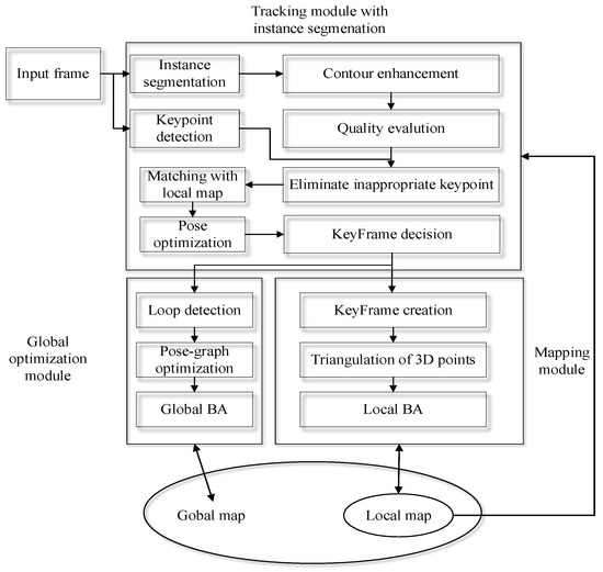
Figure 1.
Visual SLAM algorithm with pose estimation optimized by instance segmentation architecture.
We add CO-HDC instance segmentation to the tracking module, which includes the CQE contour enhancement algorithm and BAS-DP lightweight contour extraction algorithm, and use the hybrid dilated convolutional neural network as the backbone network. CO-HDC can effectively improve the accuracy of dynamic feature point segmentation, especially the contour of the target. Tracking Module with instance segmentation minimizes the impact of dynamic objects. It means that pose estimation is more accurate and keyframe decisions are better. The global optimization module and mapping module can benefit from instance segmentation, which provides high-quality feather points. Loop detection makes the global optimization module able to work well. Therefore, a more accurate map can be built.
2.1. Tracking Module with CO-HDC Instance Segmentation
According to the input RGB image and the depth image, the algorithm front end performs feature point detection and feature descriptor calculation on the RGB image. Tracking Module is divided into the following steps:
Firstly, feature matching of two adjacent frames is performed according to the feature descriptor. A 2D-2D feature matching point set is obtained. Using CO-HDC instance segmentation to remove dynamic pixels can help feature point matching greatly. The working framework of CO-HDC is shown in Figure 2, which takes the vehicle detection commonly used in the industry as an example. Among them, the backbone network adopts a hybrid dilated CNN network, which can increase the ability of network feature extraction. Then, the contour of the detected target is strengthened to improve the accuracy of instance segmentation further. At the same time, BAS-DP is used to lighten the calculation of contour, which can speed up the visual SLAM.
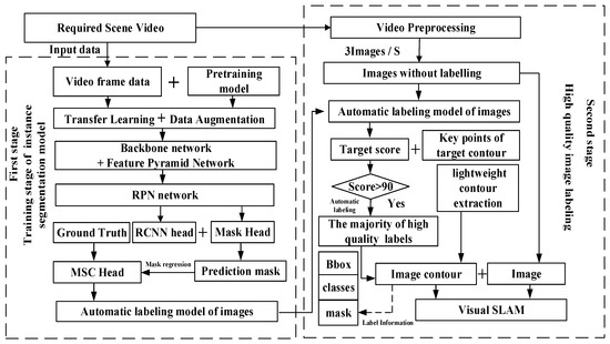
Figure 2.
Framework of CO-HDC instance segmentation.
Secondly, according to the depth information of the image, the spatial three-dimensional coordinates of the 2D-2D feature matching point pairs are calculated to obtain a 3D-3D matching point set. The rotation and translation matrix between two adjacent frames of images can be calculated from the matched 3D-3D points.
Finally, the motion estimation error is optimized to obtain the pose estimation result with the smallest error. In this way, according to the input video stream, the incremental change of the camera pose can be continuously obtained. Therefore, the front end of the algorithm constructs a visual odometer [55].
2.1.1. Complex Feature Extraction Based on Hybrid Dilated CNN
Accurate instance segmentation will be conducive to the accuracy of SLAM composition and pose estimation. In order to improve the feature extraction ability of the backbone detector in the instance segmentation model, a dilated convolutional neural network is introduced into the network. With an increase in the number of insertion holes of the dilated convolutional neural network, the size of the receptive field will increase [56], but it also leads to the loss of continuous information, which is easy to cause the problem of meshing. In order to solve the problem of continuous information loss in grid sampling, the hybrid dilated convolutional neural network can be used to replace the dilated convolutional neural network.
Suppose an n-layer convolutional neural network, and the size of the convolution kernel of each layer is . The expansion rate is . The purpose of constructing hybrid dilated convolutional neural network is that when a series of operations of dilated convolutions are completed, the extracted feature map can cover all pixels. The maximum distance between two non-zero pixels can be calculated by the following formula:
where is the expansion rate of layer , is the maximum expansion rate of layer . In order to make the final receptive field cover the whole region without any holes, an effective hybrid dilated convolutional neural network must meet . As shown in Figure 3, when the size of the convolution kernel , the expansion rate of each layer , of all pixels can be covered.
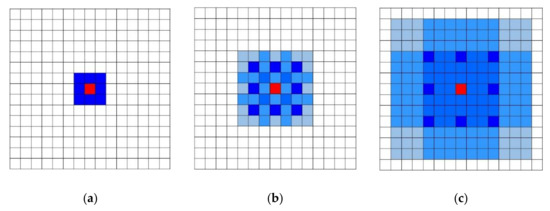
Figure 3.
Diagram of hybrid dilated convolutional neural network with different expansion rates: (a) the diagram of HDC with expansion rate 1; (b) the diagram of HDC with expansion rate 2; (c) the diagram of HDC with expansion rate 3.
In order to highlight the improvement of the performance of the instance segmentation model by the hybrid dilated convolutional neural network, the traditional convolution core is replaced by the hybrid dilated convolution core. The backbone detector structure based on the hybrid dilated convolutional neural network is shown in Figure 4.
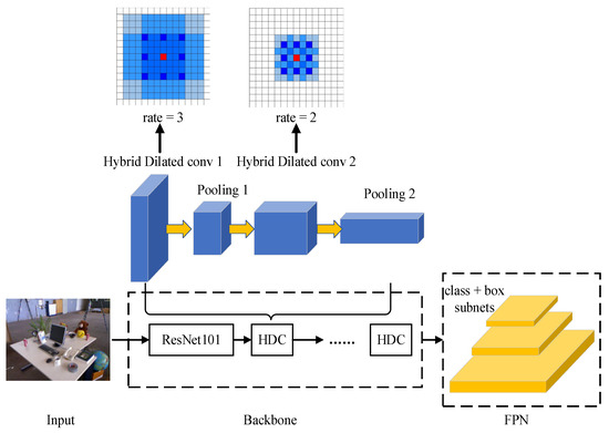
Figure 4.
The diagram of backbone detector based on hybrid dilated convolutional neural network.
2.1.2. Contour Enhancement Based on CQE
However, only the hybrid dilated convolutional neural network in the first part is not enough. Any data generation network will produce some low-quality data, especially in the contour part. If the generated data is not judged and processed, a large number of low-quality data will be mixed, and the accuracy of feature points in the later stage will be seriously affected. Therefore, CQE, a discriminator, is proposed to judge the quality of image contour. It can remove the low-quality contour information and retain the high-quality contour to enhance the contour of the object.
In most instance segmentation networks, mean intersection over union (Miou) is calculated by the ratio of their cross area to their cumulative area, and the quality of predicted contour is measured by Miou, but it is necessary to ensure that they have the same height and width. However, the Miou calculated by this method is not linear with the quality of the predicted contour, so this method is inaccurate.
Therefore, the CQE algorithm is designed, working as a discriminator to evaluate the quality of contour. The evaluation mainly includes the accuracy of the surrounding target contour and target classification accuracy. Then, by setting the quality threshold, the contour with quality lower than the threshold is discarded, and the contour with quality higher than the threshold is retained. Finally, the contour above the threshold and the corresponding image data are combined to form the instance segmentation result.
The first is to evaluate the accuracy of the target contour. Due to the irregular shape surrounding the target contour, using the regression principle in the convolutional neural network, a CQE head is designed to regress the accuracy of the target contour in the generated data, which is supervised in the process of network training, and the irregular contour is well solved. The convolutional neural network can not only extract the features in the image but can also be used to regress the similarity between the two images. The CQE head is used to regress the true contour and the predicted contour. Calculate the complete intersection over the union (Ciou) value of the difference between the real contour and the predicted contour of each target, and normalize the Ciou to obtain Siou, which is the evaluation quality of the contour. Its range is between 0 and 1. By setting different Siou thresholds, different quality target contours can be obtained. The closer the value of Siou is to 1, the better the target contour prediction effect is.
The structural design of the CQE head is composed of four convolution layers and three full connection layers. For four convolution layers, the core size and the number of filters of all convolution layers are set to 3 and 256, respectively. For three fully connected layers, set the output of the first two FC layers to 1024 to connect all neurons. The C of the last FC layer is the number of categories to be classified. Finally, the CQE head outputs the contour quality Siou of each target.
Truth-contour and Predict-contour work together as the input of the CQE head. The Truth-contour exists in the characteristic graph, and the Predict-contour is the contour output by the CQE head. Because the output result of the CQE head is different from the size of the ROI characteristic diagram, two input structures are designed. Figure 5 shows two kinds of input structures of the CQE head.
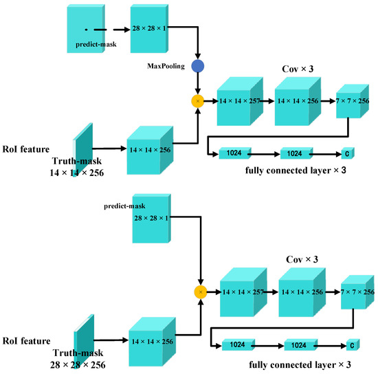
Figure 5.
Two input structures of CQE head.
Among them, the input structure designed in the first figure in Figure 5 is to maximize the pool of the feature layer output by the CQE head through a convolution kernel with a size of 2 and a step size of 2 and then multiply it with the ROI feature map with a smaller size. The input structure designed in the second figure in Figure 5 is the CQE head, which is directly added to the larger ROI characteristic diagram without maximum pooling. Both structures can be used as inputs of the CQE head. The set CQE threshold is 0.9. When the CQE of each contour in the target is higher than 0.9, the generated contour quality is higher. When the CQE of the tag contour is lower than the threshold, the generated contour quality is low. The recognition process of contour enhancement using the CQE is shown in Figure 6.
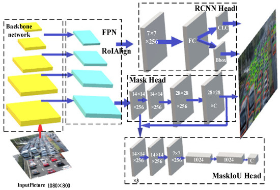
Figure 6.
The recognition structure with contour enhancement using CQE.
2.1.3. The Lightweight Contour Extraction Algorithm Based on BAS-DP
A large number of high-precision instance segmentation can be obtained through the contour enhancement network. If all points on the target contour segmented by the instance are retained, the file will be too large, which will lead to slow SLAM operation time in the later stage and make it difficult to achieve the real-time effect. Therefore, a lightweight contour extraction algorithm based on BAS-DP is proposed. The algorithm converts the contour information surrounding the target into the best polygon surrounding the target. The number of coordinate points contained in the polygon is small, which can lighten the segmentation file while ensuring the accuracy of instance segmentation.
Using the best polygon surrounding the target to replace the contour curve surrounding the target is the most direct and commonly used method. Therefore, it is necessary to convert the contour of the target into each turning point on the polygon surrounding the target. So, it is necessary to use a polygon approximation algorithm to convert the contour curve of the target into a polygon surrounding the target and then record the coordinates of key points on the polygon in the segmentation file.
Douglas–Peucker algorithm (DP algorithm) is a classical polygon approximation algorithm that can approximate the closed curve as a polygon and reduce the number of points as much as possible. It has the advantages of translation and rotation invariance. However, it needs to solve other points on the curve that do not belong to key points exhaustively, which requires a lot of calculation time. The Beetle antennae search algorithm (BA algorithm) is another classic polygon approximation algorithm that realizes efficient optimization by simulating longicorn beetle foraging. Beetle Antennae Search algorithm can realize optimization without knowing the specific form of function and gradient information. However, its accuracy is relatively low.
This paper proposes lightweight contour extraction algorithm based on BAS-DP, combining the advantages of the above two algorithms. The calculation steps are shown in Figure 7.
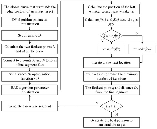
Figure 7.
The calculation steps of BAS-DP lightweight contour extraction algorithm.
In the BAS-DP algorithm, parameter initialization includes the initial trial step attenuation factor , step , the ratio of step and whisker , the number of iterations and the number of parameters to be optimized . Among them, the distance optimization function is shown in Formula (2). According to this formula, the function values and corresponding to the left whisker position and the right whisker position of the longicorn beetle can be calculated, and the next position of the longicorn beetle can be calculated at the same time. Perform calculating function n times in total. The optimal function value corresponding to the last position of the longicorn beetle is obtained as the optimal solution.
The BAS-DP algorithm can reduce the size of the segmented file while maintaining the contour accuracy and improving the real-time performance of the later visual SLAM. Finally, the BAS-DP algorithm is combined with the hybrid dilated convolutional neural network and the CQE algorithm proposed in the previous two sections, forming the CO-HDC. Through this algorithm, a large number of high-quality instance segmentation images can be generated, and the data enhancement network needs only a small amount of data to record better accuracy, especially to solve the segmentation problem of the object contour.
2.2. Pose Optimization
Through the CO-HDC algorithm, we can accurately separate the object, especially the contour of the object, removing the feature points on the dynamic object and retaining the static feature points so as to achieve good feature point matching and complete pose estimation well. In visual SLAM, posture refers to the robot in spatial position and posture of the entire environment map. Both spatial position and robot posture position need to be accurately located in the three-dimensional space.
Figure 8 shows the principle of spatial measurement. It is assumed that in two adjacent frames, the camera has no distortion, and the two projection planes are parallel and coplanar. In the figure, is an object, is its depth, is the focal length of the camera, is the center distance of two adjacent frames, and are the optical centers of two adjacent frames of the camera, respectively, and and are the horizontal axis coordinates of the projection of object in two adjacent frames, respectively. The depth calculation formula of object P can be obtained from the relationship of similar triangles:
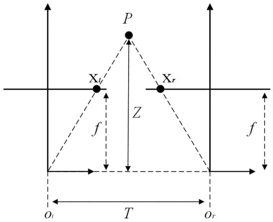
Figure 8.
The principle of spatial measurement.
is defined as parallax, so that the depth information of the target point can be obtained through the parallax and , of the target. After obtaining the parallax map, the coordinates of the target point in the world coordinate system can be obtained through the re-projection matrix. The re-projection matrix is:
In the above formula, is the coordinate value of the main point of the first frame, and is the coordinate value of the main point of the second frame. Assuming that the identified coordinate of the target point is , and the parallax in the two adjacent frames is , its coordinate value in the world coordinate system can be recovered through Formula (5):
In proposed SLAM, the robot’s posture is calculated through the translation vector and rotation quaternion number representation of seven paraments, as shown in the following type (6):
The first three are translation vectors. The last quaternion is the quaternion for rotation.
The task of the tracking thread is to calculate the posture of two adjacent frames according to the image change. This means not only the distance moved in the next frame should be calculated, but also the angle of rotation should be calculated. The results are then handed over to the back end, which accumulates and optimizes the relative positions between the two frames.
The images obtained by the pre-recognition before and after are and . After feature extraction, the feature point is obtained in . The feature point is obtained in . Assuming the result of feature matching is that is obtained and is the closest point pair, it means that and is the projection of the same 3D point P on two frames of images.
where, is the camera’s internal parameter matrix. When the camera is in different positions, point obtains different pixel coordinates through the transformation of the internal parameter matrix. They are projection and . is the pose of relative to . Assuming that multiple sets of point pairs can be matched between the two frames, the equation can be constructed by these point pairs to solve the relative pose. Specifically, it can be solved by solving the basis matrix and the homology matrix.
However, must be calculated in the space, where the whole environment’s stationary conditions are valid. If the points in the pose estimation are in the process of moving, type (4) is set up. The error would arise. The worst-case scenario is to use the camera to participate in the pose estimation of all pixels for the same shipment. Then the pose estimation will always be 0.
2.3. Global Optimization Module and Mapping Module
The tracking module estimates the camera poses through keypoint matching and pose optimization. An instance segmentation function is added to the tracking thread, and the original image is segmented at the same time as the feature extraction. Then, the pixel coordinates of the human and the animal are obtained. Finally, some feature points distributed on the human or animal are removed from the original feature point.
After culling feature points, the feature matching and pose estimation are performed. After getting rid of the interference of the pixel points, the instance SLAM shows better anti-interference ability under dynamic scenes. The accuracy is greatly improved. This module also determines whether to insert a new keyframe. When a frame is considered suitable for a new keyframe, it is sent to the mapping module and global optimization module.
In the mapping module, to eliminate mismatches or inaccurate matches, a new 3D point is triangulated by inserting a keyframe, optimizing the projected points and lines and adding a projection matrix. This process is equivalent to minimizing the photometric difference between blocks of projected pixels and the blocks corresponding to the 3D point on the current frame . The model expression is:
where, and are the first and second frames, respectively, and is the projection matrix. The projection matrix formula is as follows:
where, is the matrix representing rotation and scaling, and are the coordinates before projection, and and represent translation distance.
In the process of global optimization, it is necessary to eliminate the accumulated errors caused by the odometer. The matching algorithm we use is a kind of image matching based on pixel value. Its purpose is to find a strict geometric transformation to make each pixel in the local map and the global map equal as much as possible. The inverse compositional algorithm can solve the problem of image matching, which is completed in three steps. The specific steps are given in the following formulations:
The first step is to calculate the Hessian matrix H:
where, is the global map image, is the coordinates of pixels in the image, represents translation and rotation vectors, and represents the Euclidean transformation of vector on image I(x).
The second step is to calculate the new vector ∆ p:
where, is the image of a local subgraph.
Step 3: Update vector :
The final output of the algorithm represents the translation and rotation between maps, which can eliminate the accumulated errors in global map construction, and also solves the problem of trajectory drift that often occurs in visual SLAM.
3. Tests and Results Analysis
In order to demonstrate the advantages of the CO-HDC instance segmentation algorithm proposed in this paper and test the actual effect of visual SLAM based on CO-HDC instance segmentation, our experiment will be divided into two parts. Firstly, we will experiment with the performance of the CO-HDC instance segmentation algorithm. Secondly, we will test the performance of the visual SLAM based on the CO-HDC instance segmentation algorithm proposed in this paper and judge the effect of feature point matching and real-time modeling.
3.1. Experiment of CO-HDC Instance Segmentation Algorithm
In order to test the accuracy and efficiency of the proposed contour enhancement instance segmentation algorithm, the following experiments are carried out:
- the selection of network hyperparameters to achieve the precise and fast segmentation;
- comparison of different backbone networks.
3.1.1. The Network Hyperparameters Selection and Controlled Experiment
Instance segmentation can remove the dynamic object, which increases the accuracy of visual SLAM. In order to integrate with visual SLAM better, the instance segmentation network model needs to be optimized. Therefore, ten comparative experiments were conducted under hybrid dilated CNN to select appropriate network parameters and observe the effect of transfer learning on training time, accuracy and training data volume. The hyperparameters selection and the corresponding results are shown in Table 3. mAP is the average precision, and mIoU is the average intersection ratio. In this paper, mAP and mIoU are used to evaluate the quality of network training structure. In order to strictly evaluate the performance of the method, the thresholds of mAP are set to 0.5 and 0.7, respectively. Those greater than or equal to the threshold are true positive, while those less than the threshold are false positive. The mIoU and mAP indicators for each experiment are shown in the last three rows of the table for detailed analysis of the experiment contents and results.

Table 3.
Hyperparameters selection comparison experiments.
Train obj. and Val obj. correspond to the total number of training objectives and verification objectives of the training, respectively. Train imag. and Val imag. are the number of training images and verification images. Epochs is the number of iterations of all training sets, and the Mini-mask Shape is the minimum mask size. Img. Size is the size of the input image, and RPN Anchor Scales is the proportion Size of the Anchor. The Pretrain Model is the 80 classification pre-training model of coco data sets.
Test 1 and Test 2 use the same Non-Maximum Suppression (NMS) threshold, the basic learning rate, and other hyperparameters but use different amounts of epochs. Feeding all data into the network for iteration is called an epoch, and the number of epochs is set to 100 and 200, respectively. With the increase of epochs, the value of mAP (IoU > 0. 5) in test 1 increased from 0.569 to 0.586 with a low volatility effect. So, on a low number of iterations, it was still easy to converge, indicating that the convergence effect of the algorithm in this paper was great.
In Test 3 and Test 6, we used images of more data for training and testing, and epochs were the same as before. The results showed a decrease in detection rate, which was later improved in test 4 by increasing the number of epochs, resulting in an mAP (IoU > 0. 5) of 0. 565.
In Test 5, we evaluate the effects of the image width and height, the size of the training images from 1024 × 800 to 1920 × 1080, learning rate from the default of 0. 001 to 0. 02, the rest of the parameters like Test 4. We get a poor performance of the algorithm (mAP (IoU > 0. 5) = 0.395). It indicates that the accuracy of images of high resolution is low under the current parameters.
In Test 6, we reduced the size of the mini-mask from 56 × 56 to 28 × 28, and compared with Test 4; we found some improvement in network performance.
Therefore, in Test 7, we reduced the Scales of RPN Anchor and improved the input image resolution to 1920 × 1080 and the small mask to 28 × 28. It was found that the performance of the network was greatly improved, which was close to the network performance in Test 6.
In Test 8, we used the same configuration as Test 7 and further reduced the RPN Anchor Scales. It was found that the performance of the network with reduced RPN Anchor Scales was greatly improved, and (8, 16, 32, 64) was considered the best RPN Anchor Scales of the network.
In Test 9, in order to improve the training accuracy, reduce the training time and prevent network overfitting, we reduced the amount of training data on the basis of Test 8 and found that the network performance decreased significantly.
In Test 10, we substantially recompressed the training data on the basis of Test 9, other parameters remained unchanged, and we used 80 classification models of the pre-trained COCO data sets for transfer learning. The results showed that the network performance was basically the same as that of Test 8, and the network performance reached a higher level, but the training time was half that of Test 8. Network performance can accurately detect and segment vehicle images.
Through 10 comparative experiments, it can be seen that the more training data, the higher the image resolution, the smaller the mask and the smaller the scale of RPN anchor will lead to better network performance. The results show that 100 epochs are enough to achieve convergence for target detection. At the same time, an increasing pre-training model can reduce the training data. In conclusion, Test 10 achieves the most perfect balance among training data, image resolution, mask size, epochs, scale of the RPN anchor and other parameters. Appropriate data volume and resolution ensure not only high speed but also high precision. At the same time, the transfer learning method can reduce the training data, training time and improve the detection accuracy. Therefore, we set the parameters of Test 10 as our optimal network parameters and carried out subsequent experiments and studies with the parameters of Test 10.
3.1.2. Comparison of Different Backbone Networks
Under the network configuration parameters of Test 10, a comparative test was conducted for different backbone networks to demonstrate the advantages of HDC-Net. The neural networks of HDC-Net, ResNet50, Res-Net101 and MobileNetV1 were all composed of residual blocks, which simplified their architectures with residual learning, reduced their computational overhead and well solved the gradient vanishing problem.
Its performance was compared in four aspects. Network training time, image detection time per second, network model weight and accuracy (S > 90 means that SMask is greater than 90). Accuracy is the ratio of high-quality labels to all labels. It can be seen from the Table 4 that when HDC-Net is used as the backbone network, the training time is 13.21 h, which is quite similar to ResNet50; the speeds of these four networks are 6.65 sheets per second, 6.25 sheets per second, 4.6 sheets per second and 5.2 sheets per second respectively, and HDC-Net has the fastest speed for calibrating the image. In the model size comparison test, when HDC-Net is used as the backbone network, the label model size is the smallest. When HDC-Net, ResNe50, ResNet101 and MobileNet V1 are used as the backbone network, the accuracy of the vehicle image label is 95.1%, 93.4%, 93.8% and 84.5%, respectively. It can be seen that although HDC-Net has a slight increase in training time compared with ResNet50, it is far ahead of other backbone networks in terms of speed, model weight and accuracy. Therefore, HDC-Net has the best performance.

Table 4.
Performance comparison of four backbone networks.
3.2. Experiment of Visual SLAM Based on CO-HDC
In this paper, two sets of tests are carried out to evaluate the visual SLAM based on CO-HDC. The first set of tests is that dynamic feature points for single-frame pictures in motion and intermediate results are shown. The second set of tests is that the instance visual SLAM based on CO-HDC proposed in this paper and ORB-SLAM2 algorithms are run on the TUM RGBD public dataset. Other than this, experimental results are compared with each other.
The dataset used in this paper are rgbd_dataset_freiburg3_walking_xyz (dataset one), rgbd_dataset_freiburg3_walking_halfsphere (dataset two) and rgbd_dataset_freiburg3_walking_static (dataset three) in the TUM dataset Dynamic Objects. This dataset contains moving people, and the camera is also in motion to evaluate the robustness of the SLAM system or motion calculations in scenes with fast-moving dynamic objects. In the dataset, the video frame rate is 30 Hz, and the sequence contains a full sensor resolution is 640 × 480. The ground real trajectory is obtained from a motion capture system of eight high speed tracking cameras.
3.2.1. Feature Point Extraction and Matching after CO-HDC Instance Segmentation
A comparison between ORB-SLAM2 and the proposed visual SLAM based on CO-HDC instance segmentation is carried out. ORB-SLAM2 assumes that feature points in the scenes are static, and feature points matching is performed directly after feature points extraction. However, this may lead to pose estimation errors and map relative drifts under dynamic environments. At the same time, the proposed visual SLAM segments the dynamic objects and retains static feature points. Moreover, it performs feature points matching using static point only.
Firstly, the feature point extraction and matching in the ORB-SLAM2 algorithm are performed. The two adjacent frames in the video sequence of the dataset are randomly selected, as shown in Figure 9a,b. Figure 9c,d show the feature extraction in the ORB-SLAM2 algorithm, where some feature points fall on the human body. Then, the feature matching is shown in Figure 9e.
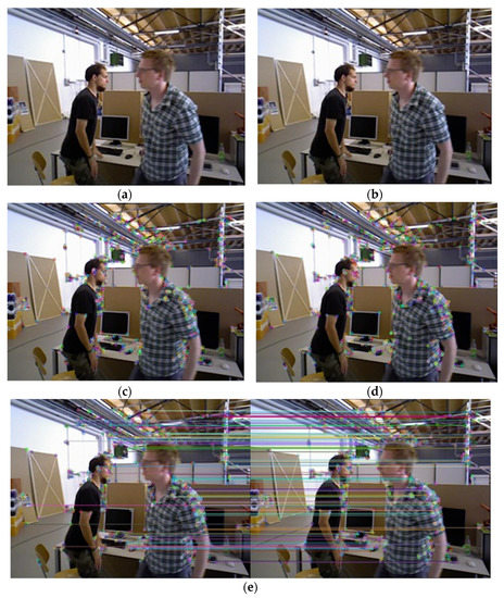
Figure 9.
Results of feature extraction and matching based on ORB-SLAM2: (a) Original Figure 1; (b) Original Figure 2; (c) Feature points extracted before screening of original Figure 1; (d) Feature points extracted before screening of original Figure 2; (e) The ORB matching results of original Figure 1 and Figure 2.
The processing results based on the method proposed in this paper are shown in Figure 10. Areas in the image are visualized where feature points are removed, as shown in Figure 10a,b. It can be seen that the extracted feature points fall on the human body before the instance segmentation. After the instance segmentation and screening, the feature points falling on the human body are removed in Figure 10c,d. In the subsequent pose estimation, these feature points will be ignored, greatly increasing the accuracy of pose estimation, which is shown in Figure 10e.
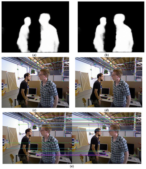
Figure 10.
Results of feature extraction and matching based on proposed SLAM: (a) Figure for dynamic dot culling of first frame; (b) Figure for dynamic dot culling of second frame; (c) Feature points extracted after screening of first frame; (d) Feature points extracted after screening of second frame; (e) The ORB matching results of original Figure 1 and Figure 2 after screening.
3.2.2. Using Datasets to Test the Preference of ORB-SLAM2 and Instance Visual SLAM Based on CO-HDC Algorithm
The dataset provides an automated assessment tool for visual odometer system drift and global attitude error for SLAM systems, which is divided into absolute trajectory errors (ATE) and relative pose errors (RPE). The ATE difference is used to calculate the difference between the actual values and estimated values of the camera pose of the SLAM system. The RPE is used to calculate the difference between the pose changes on the same two timestamps. Firstly, the estimated value is aligned with the real value according to the timestamp of the pose. The drift of the system is also evaluated. From Figure 11, Figure 12 and Figure 13, the RPE of instance SLAM based on CO-HDC is much smaller than ORB-SLAM2. The amount of change in pose is calculated at the same time. From Figure 14, Figure 15 and Figure 16, it can be concluded that the proposed SLAM performs better than ORB-SLAM2, as the ATE of the proposed SLAM is also smaller than ORB-SLAM2. In Table 5, compared with ORB-SLAM2, the Rmse of the proposed method in absolute trajectory error is about 30 times smaller and is only 0.02 m. The comparison in Table 6 and Table 7 also confirms the advantages of the proposed SLAM.
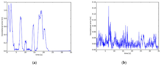
Figure 11.
Relative pose error of dataset one: (a) The relative pose error of dataset one using ORB-SLAM2; (b) The relative pose error of dataset one using instance SLAM based on CO-HDC.
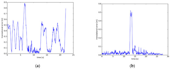
Figure 12.
Relative pose error of dataset two: (a) The relative pose error of dataset two using ORB-SLAM2; (b) The relative pose error of dataset two using instance SLAM based on CO-HDC.
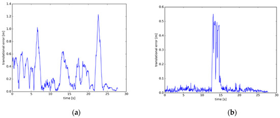
Figure 13.
Relative pose error of dataset three: (a) The relative pose error of dataset two using ORB-SLAM2; (b) The relative pose error of dataset two using instance SLAM based on CO-HDC.
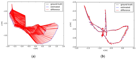
Figure 14.
Absolute trajectory error of dataset one: (a) The absolute trajectory error of dataset one using ORB-SLAM2; (b) The absolute trajectory error of dataset one using instance SLAM based on CO-HDC.
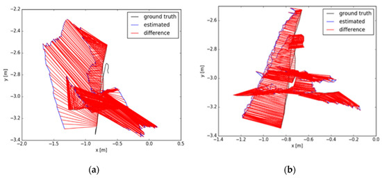
Figure 15.
Absolute trajectory error of dataset two: (a) The absolute trajectory error of dataset two using ORB-SLAM2; (b) The absolute trajectory error of dataset two using instance SLAM based on CO-HDC.
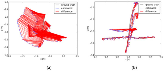
Figure 16.
Absolute trajectory error of dataset three: (a) The absolute trajectory error of dataset two using ORB-SLAM2; (b) The absolute trajectory error of dataset two using instance SLAM based on CO-HDC.

Table 5.
Pose error representative value of dataset one.

Table 6.
Pose error representative value of dataset two.

Table 7.
Pose error representative value of dataset three.
The platform of this experiment is a personal laptop configured as CPU I7 7700HQ, GPU 1050TI and 16G memory. The evaluation tool is used to compare the errors of the two systems running the above two datasets.
Through the above experiments, comparing ORB-SLAM2 and instance SLAM based on CO-HDC, we can see that the performance of instance SLAM based on CO-HDC is better than traditional SLAM.
4. Discussion
Visual SLAM based on instance segmentation has been widely used due to its high accuracy in dynamic environments. At present, eliminating dynamic feature points to improve the accuracy of visual SLAM is a widely recognized method in academic circles [57,58]. Alejo Concha et al. use this technology to prolong the time of world-locked mobile AR experiences, letting users have a more satisfying experience [59]. Fessl [60] and Sanchez-Lopez [61] et al. have applied them in the field of aircraft. In addition, it has been widely used in location-aware communication [62], medical [6], 3D printing [5] and other fields [63]. However, this method has two major problems: the accuracy of dynamic point elimination is not high, and the elimination speed is slow. To solve these two problems, we propose a CO-HDC instance segmentation model, which consists of a CQE contour enhancement algorithm and a BAS-DP lightweight contour extraction algorithm.
Firstly, the main reason for the low accuracy of dynamic feature point elimination is the low accuracy of object contour segmentation, which makes it difficult to distinguish whether the feature points at the object contour are dynamic feature points or static feature points. To solve this problem, we propose a CQE contour enhancement algorithm. By evaluating the contour of the object, the optimal contour is selected as the output. In order to solve this problem, Chang et al. introduced the optical flow method to detect moving objects [64]. The optical flow method obtains the motion information of the object by calculating the change of pixels between adjacent frames. This method can not only work when the camera is in motion but also get the three-dimensional structure of the object. However, the optical flow method is too sensitive to the change of illumination intensity, and it needs to assume that the brightness of object pixels is constant. This is difficult to achieve in most cases. In addition, the optical flow method is difficult to recognize fast-moving objects. Therefore, in contrast, the method proposed in this paper has stronger robustness and can better adapt to a complex environment.
Secondly, in order to match the mapping speed of visual SLAM based on instance segmentation, instance segmentation needs to have a faster segmentation speed. The BAS-DP lightweight contour extraction algorithm proposed in this paper can effectively reduce the amount of calculation while ensuring accuracy by using the most similar polygon contour. In order to solve the same problem, Xiong et al. optimized the backbone network and accelerated the segmentation speed by designing a semantic segmentation head based on deformable convolution [65]. However, this method depends on the selection of keyframes in the video sequence. Therefore, compared with it, the method proposed in this paper is more practical.
5. Conclusions
This paper has presented a pose estimation optimized visual SLAM algorithm based on the CO-HDC instance segmentation network for dynamic scenes. CO-HDC instance segmentation includes the CQE contour enhancement algorithm and the BAS-DP lightweight contour extraction algorithm. The CQE contour enhancement algorithm improves the segmentation accuracy at the contour of dynamic objects. The problem of excessive calculation of instance segmentation is overcome by the BAS-DP algorithm. As the test results show, the proposed algorithm can reduce pose estimation errors and map relative drifts under dynamic environments compared to ORB-SLAM2.
In the future, visual SLAM based on instance segmentation has broad development space, including the driverless field, 3D printing industry, location-aware communication, aircraft and other fields. Instance segmentation can not only improve the accuracy of visual SLAM but also provide rich object information in the scene. In future work, the proposed algorithm would be further implemented and demonstrated in the embedded system to fit more robots under complex environments.
Author Contributions
Conceptualization, J.C. and F.X.; methodology, J.C., F.X. and L.H.; software, F.X. and X.L.; validation, J.C., F.X., J.Y. and J.S.; formal analysis, F.X.; investigation, X.L. and J.S.; resources, L.H. and J.Y.; data curation, X.L.; writing—original draft preparation, J.C. and F.X.; writing—review and editing, J.C., F.X. and X.L.; visualization, J.S.; supervision, J.Y.; project administration, F.X.; funding acquisition, J.Y. and J.S. All authors have read and agreed to the published version of the manuscript.
Funding
This work was partially supported by the National Natural Science Foundation of China (Grant No. 41974033), the Scientific and Technological Achievements Program of Jiangsu Province (BA2020004), and 2020 Industrial Transformation and Upgrading Project of Industry and Information Technology Department of Jiangsu Province (JITC-2000AX0676-71), Postgraduate Research & Practice Innovation Program of Jiangsu Province.
Data Availability Statement
Publicly available datasets were analyzed in this study, 2 April 2022. The dataset can be found here: https://vision.in.tum.de/data/datasets/rgbd-dataset/download (accessed on 12 March 2022).
Conflicts of Interest
The authors declare no conflict of interest.
References
- García-Fernández, Á.F.; Hostettler, R.; Särkkä, S. Rao-Blackwellized Posterior Linearization Blackward SLAM. IEEE Trans. Veh. Technol. 2019, 68, 4734–4747. [Google Scholar] [CrossRef]
- Evers, C.; Naylor, P.A. Optimized Self-localization for SLAM in Dynamic Scenes Using Probability Hypothesis Density filters. IEEE Trans. Signal Process. 2018, 66, 863–878. [Google Scholar] [CrossRef] [Green Version]
- Lee, J.; Hwang, S.; Kim, W.J.; Lee, S. SAM-Net: LiDAR Depth Inpainting for 3D Static Map Generation. IEEE Trans. Intell. Transp. Syst. 2021, 22, 1–16. [Google Scholar] [CrossRef]
- Cattaneo, D.; Vaghi, M.; Valada, A. LCDNET: Deep Loop Closure Detection and Point Cloud Registration for Lidar SLAM. IEEE Trans. Robot. 2022, 38, 1–20. [Google Scholar] [CrossRef]
- Li, J.; Aubin-Fournier, P.L.; Skonieczny, K. SLAAM: Simultaneous Localization and Additive Manufacturing. IEEE Trans. Robot. 2021, 37, 334–349. [Google Scholar] [CrossRef]
- Hussain, A.; Memon, A.R.; Wang, H.; Wang, Y.; Miao, Y.; Zhang, X. S-VIT: Stereo Visual-Inertial Tracking of Lower Limb for Physio therapy Rehabilitation in Context of Comprehensive Evaluation of SLAM Systems. IEEE Trans. Autom. Sci. Eng. 2021, 19, 1550–1562. [Google Scholar] [CrossRef]
- Mur-Artal, R.; Tardós, J.D. ORB-SLAM2: An Open-Source SLAM System for Monocular, Stereo, and RGB-D Cameras. IEEE Trans. Robot. 2017, 33, 1255–1262. [Google Scholar] [CrossRef] [Green Version]
- Shi, Q.; Zhao, S.; Cui, X.; Lu, M.; Jia, M. Anchor self-localization algorithm based on UWB ranging and inertial measurements. Tsinghua Sci. Technol. 2019, 24, 728–737. [Google Scholar] [CrossRef]
- Yang, S.; Scherer, S. Monocular Object and Plane SLAM in Structured Environments. IEEE Robot. Autom. Lett. 2019, 4, 3145–3152. [Google Scholar] [CrossRef] [Green Version]
- Han, F.; Wang, H.; Huang, G.; Zhang, H. Sequence-based sparse optimization methods for long-term loop closure detection in visual SLAM. Auton. Robot. 2018, 42, 1323–1335. [Google Scholar] [CrossRef]
- Yuan, J.; Zhu, W.; Dong, X.; Sun, F.; Zhang, X.; Sun, Q.; Huang, Y. A Novel Approach to Inage-Sequence-Based Mobile Robot Place Recognition. IEEE Trans. Syst. 2021, 51, 5377–5391. [Google Scholar]
- Ntalampiras, S. Moving Vehicle Classification Using Wireless Acoustic Sensor Networks. IEEE Trans. Eng. Top. Comput. Intell. 2018, 2, 129–138. [Google Scholar] [CrossRef]
- Zhu, J.; Jia, Y.; Li, M.; Shen, W. A New System to Construct Dense Map with Pyramid Stereo Matching Network and ORB-SLAM2. In Proceedings of the International Conference on Computer and Communications, Chengdu, China, 10–13 December 2021; pp. 430–435. [Google Scholar]
- Fan, T.; Wang, H.; Rubenstein, M.; Murphey, T. CPL-SLAM: Efficient and Certifiably Correct Planar Graph-Based SLAM Using the Complex Number Representation. IEEE Trans. Robot. 2020, 36, 1719–1737. [Google Scholar] [CrossRef]
- Han, L.; Xu, L.; Bobkov, D.; Steinbach, E.; Fang, L. Real-Time Global Registration for Globally Consistent RGB-D SLAM. IEEE Trans. Robot. 2019, 35, 498–508. [Google Scholar] [CrossRef]
- Gomez-Ojeda, R.; Moreno, F.A.; Zuniga-Noël, D.; Scaramuzza, D.; Gonzalez-Jimenez, J. PL-SLAM: A Stereo SLAM System through the Combination of Points and Line Segments. IEEE Trans. Robot. 2019, 35, 734–746. [Google Scholar] [CrossRef] [Green Version]
- Gao, H.; Zhang, X.; Yuan, J.; Song, J.; Fang, Y. A Novel Global Localization Approach Based on Structual Unit Encoding and Multiple Hypothesis Tracking. IEEE Trans. Instrum. Meas. 2019, 68, 4427–4442. [Google Scholar] [CrossRef]
- Gao, H.; Zhang, X.; Wen, J.; Yuan, J.; Fang, Y. Autonomous Indoor Exploration Via Polygon Map Construction and Graph-Based SLAM Using Directional Endpoint Features. IEEE Trans. Autom. Sci. Eng. 2019, 16, 1531–1542. [Google Scholar] [CrossRef]
- Xie, Y.; Zhang, Y.; Chen, L.; Cheng, H.; Tu, W.; Cao, D.; Li, Q. RDC-SLAM: A Real-Time Distributed Cooperative SLAM System Based on 3D LiDAR. IEEE Trans. Intell. Transp. Syst. 2021, 22, 1–10. [Google Scholar] [CrossRef]
- Guo, C.X.; Sartipi, K.; DuToit, R.C.; Georgiou, G.A.; Li, R.; O’Leary, J.; Nerurkar, E.D.; Hesch, J.A.; Roumeliotis, S.I. Resource-Aware Large- Scale Cooperative Three -Dimensional Mapping Using Multiple Mobile Devices. IEEE Trans. Robot. 2018, 34, 1349–1369. [Google Scholar] [CrossRef]
- Zhang, Y.; Chen, L.; Zhe, X.; Tian, W. Three-Dimensional Cooperative Mapping for Connected and Automated Vehicles. IEEE Trans. Ind. Elecronice 2020, 67, 6649–6657. [Google Scholar] [CrossRef]
- Chu, X.; Lu, Z.; Gesbert, D.; Wang, L.; Wen, X. Vehicle Localization via Cooperative Channel Mapping. IEEE Trans. Veh. Technol. 2021, 70, 5719–5733. [Google Scholar] [CrossRef]
- Yassin, A.; Nasser, Y.; Al-Dubai, A.Y.; Awad, M. MOSAIC: Simultaneous Localization and Environment Mapping Using nnWave Without A-Priori Knowledge. IEEE Access 2018, 6, 68932–68947. [Google Scholar] [CrossRef]
- De Lima, C.; Belot, D.; Berkvens, R.; Bourdoux, A.; Dardari, D.; Guillaud, M.; Isomursu, M.; Lohan, E.-S.; Miao, Y.; Barreto, A.N.; et al. Convergent Communication, Sensing and Localization in 6G Systems: An Overview of Technologies, Opportunities Challenges. IEEE Access 2021, 9, 26902–26925. [Google Scholar] [CrossRef]
- Aladsani, M.; Alkhateeb, A.; Trichopoulos, G.C. Leveraging mmWAVE Imaging and Communications for Simultaneous Localization and Mapping. In Proceedings of the 2019 IEEE International Conference on Acoustics, Speech and Signal Processing (ICASSP), Brighton, UK, 12–17 May 2019; pp. 4539–4543. [Google Scholar]
- Fascista, A.; Coluccia, A.; Wymeersch, H.; Seco-Granados, G. Downlink Single-Snapshot Localization and Mapping with a Single-Antenna Receiver. IEEE Trans. Wirel. Commun. 2021, 20, 4672–4684. [Google Scholar] [CrossRef]
- Saputra, M.R.U.; Lu, C.X.; de Gusmao, P.P.B.; Wang, B.; Markham, A.; Trigoni, N. Graph-Based Thermal-Inertial SLAM With Probabilistic Neural Networks. IEEE Trans. Robot. 2021, 37, 1–19. [Google Scholar] [CrossRef]
- Poulose, A.; Han, D.S. Hybrid Indoor Localization Using IMU Sensors and Smartphone Camera. Sensors 2019, 19, 5084. [Google Scholar] [CrossRef] [PubMed] [Green Version]
- Jung, J.H.; Choe, Y.; Park, C.G. Photometric Visual-Inertial Navigation with Uncertainty-Aware Ensembles. IEEE Trans. Robot. 2021, 37, 1–14. [Google Scholar] [CrossRef]
- Campos, C.; Elvira, R.; Rodríguez, J.J.G.; Montiel, J.M.; Tardós, J.D. ORB-SLAM3: An Accurate Open-Source Library for Visual, Visual-Inertial, and Multimap SLAM. IEEE Trans. Robot. 2021, 37, 1874–1890. [Google Scholar] [CrossRef]
- Muñoz-Salinas, R.; Medina-Carnicer, R. UcoSLAM: Simultaneous localization and mapping by fusion of keypoints and squared planar markers. Pattern Recognit. 2020, 101, 107193. [Google Scholar] [CrossRef] [Green Version]
- Ding, X.; Wang, Y.; Xiong, R.; Li, D.; Tang, L.; Yin, H.; Zhao, L. Persistent Stereo Visual Localization on Cross-Modal Invariant Map. IEEE Trans. Intell. Transp. Syst. 2020, 21, 4646–4658. [Google Scholar] [CrossRef]
- Chou, C.C.; Chou, C.F. Efficient and Accurate Tightly-Coupled Visual-Lidar SLAM. IEEE Trans. Intell. Transp. Syst. 2021, 22, 1–15. [Google Scholar] [CrossRef]
- Wu, Y.; Li, Y.; Li, W.; Li, H.; Lu, R. Robust Lidar-Based Localization Scheme for Unmanned Ground Vehicle via Multisensor Fusion. IEEE Trans. Neural Netw. Learn. Syst. 2021, 32, 5633–5643. [Google Scholar] [CrossRef] [PubMed]
- Li, J.; Hu, S.; Li, Q.; Chen, J.; Leung, V.C.; Song, H. Global Visual and Semantic Observations for Outdoor Robot Localization. IEEE Trans. Netw. Sci. Eng. 2021, 8, 2909–2921. [Google Scholar] [CrossRef]
- Han, S.; Xi, Z. Dynamic scene semantics SLAM based on semantic segmentation. IEEE Access 2020, 8, 43563–43570. [Google Scholar] [CrossRef]
- Li, F.; Chen, W.; Xu, W.; Huang, L.; Li, D.; Cai, S.; Yang, M.; Xiong, X.; Liu, Y.; Li, W. A mobile robot visual SLAM system with enhanced semantics segmentation. IEEE Access 2020, 8, 25442–25458. [Google Scholar] [CrossRef]
- Zhang, Z.; Zhang, J.; Tang, Q. Mask R-CNN based on semantic RGB-D SLAM for dynamics scenes. In Proceedings of the IEEE International Conference on Advanced Intelligent Mechatronics, Hong Kong, China, 8–12 July 2019; pp. 1151–1156. [Google Scholar]
- Ai, Y.; Rui, T.; Lud, M.; Fu, F.; Liu, S.; Wang, S. DDL-SLAM: A robust RGB-D SLAM in dynamic environments combined with deep learning. IEEE Access 2020, 8, 162335–162342. [Google Scholar] [CrossRef]
- Javed, Z.; Kim, G.-W. A comparative study of recent real time semantic segmentation algorithms for visual semantic SLAM. In Proceedings of the IEEE International Conference on Big Date and Smart Computing, Online, 10–13 December; pp. 474–476.
- Qian, H.; Ding, P. An improved ORB-SLAM2 in dynamic scene with instance segmentation. In Proceedings of the International Workshop on Research, Education and Development on Unmanned Aerial Systems, Cranfield, UK, 25–27 November 2019; pp. 185–191. [Google Scholar]
- Bolya, D.; Zhou, C.; Xiao, F.; Lee, Y.J. YOLACT Real-time Instance Segmentation. In Proceedings of the IEEE International Conference on Computer Vision, Seoul, Korea, 27 October–2 November 2019; pp. 9157–9166. [Google Scholar]
- Bista, S.R.; Hall, D.; Talbot, B.; Zhang, H.; Dayoub, F.; Sünderhauf, N. Evaluating the impact of semantic segmentation and pose estimation on dense semantic SLAM. In Proceedings of the IEEE International Conference on Intelligent Robots and Systems, Prague, Czech Republic, 27 September–1 October 2021; pp. 5328–5335. [Google Scholar]
- Yu, C.; Liu, Z.; Liu, X.J.; Xie, F.; Yang, Y.; Wei, Q.; Fei, Q. DS-SLAM: A Semantic Visual SLAM towards Dynamic Environments. In Proceedings of the IEEE International Conference on Intelligent Robots and Systems (IROS), Madrid, Spain, 1–5 October 2018; pp. 1168–1174. [Google Scholar]
- Wu, Y.; Luo, L.; Yin, S.; Yu, M.; Qiao, F.; Huang, H.; Shi, X.; Wei, Q.; Liu, X. An FPGA Based Energy Efficient DS-SLAM Accelerator for Mobile Robots in Dynamic Environment. Appl. Sci. 2021, 11, 1828. [Google Scholar] [CrossRef]
- Bescos, B.; Fácil, J.M.; Civera, J.; Neira, J. DynaSLAM: Tracking, Mapping, and Inpainting in Dynamic Scenes. IEEE Robot. Autom. Lett. 2018, 3, 4076–4083. [Google Scholar] [CrossRef] [Green Version]
- Bescos, B.; Campos, C.; Tardós, J.D.; Neira, J. DynaSLAM II: Tightly-Coupled Multi-Object Tracking and SLAM. IEEE Robot. Autom. Lett. 2021, 6, 5191–5198. [Google Scholar] [CrossRef]
- Endo, Y.; Sato, K.; Yamashita, A.; Matsubayashi, K. Indoor Positioning and Obstacle Detection for Visually Impaired Navigetion System based on LSD-SLAM. In Proceedings of the International Conference on Biometrics and Kansei Engineering, Kyoto, Japan, 15–17 September 2017; pp. 158–162. [Google Scholar]
- Cui, L.; Ma, C. SOF-SLAM: A Semantic Visual SLAM for Dynamic Environments. IEEE Access 2019, 7, 166528–166539. [Google Scholar] [CrossRef]
- Whelan, T.; Leutenegger, S.; Salas-Moreno, R.; Ben, G.; Davison, A. ElasticFusion: Dense SLAM without A Pose Graph. In Proceedings of the Conference on Robotics—Science and Systems, Rome, Italy, 13–17 July; pp. 1–23.
- Ran, T.; Yuan, L.; Zhang, J.; Tang, D.; He, L. RS-SLAM: A robust semantic SLAM in dynamic environment based on RGB-D sensor. IEEE Sens. J. 2021, 21, 20657–20664. [Google Scholar] [CrossRef]
- Ballester, I.; Fontan, A.; Civera, J.; Strobl, K.H.; Triebel, R. DOT: Dynamic object tracking for visual SLAM. In Proceedings of the IEEE International Conference on Robotics and Automation, Xi’an, China, 31 May–4 June 2021; pp. 11705–11711. [Google Scholar]
- Mingachev, E.; Lavrenov, R.; Tsoy, T.; Matsuno, F.; Svinin, M.; Suthakorn, J.; Magid, E. Comparison of ROS-Based Monocular Visual SLAM Methods: DSO, LDSO, ORB-SLAM2 and DynaSLAM. In Proceedings of the Interactive Collaborative Robotics, St Petersburg, Russia, 7–9 October 2020; pp. 222–233. [Google Scholar]
- Xia, L.; Cui, J.; Shen, R.; Xu, X.; Gao, Y.; Li, X. A survey of image semantics-based visual simultaneous localization and mapping: Application-oriented solutions to autonomous navigation of mobile robots. Int. J. Adv. Robot. Syst. 2020, 17, 1–17. [Google Scholar] [CrossRef]
- Sun, Y.; Liu, M.; Meng, M.Q.-H. Improving RGB-D SLAM in dynamic environments: A motion removal approach. Robot. Auton. Syst. 2017, 89, 110–122. [Google Scholar] [CrossRef]
- Xie, X.; Li, C.; Yang, X.; Xi, J.; Chen, T. Dynamic Receptive Field-Based Object Detection in Aerial Imaging. Acta Opt. Sin. 2020, 40, 0415001. [Google Scholar]
- Dong, X.; Ouyang, Z.; Guo, Z.; Niu, J. Polarmask-tracker: Lightweight multi-object tracking and segmentation model for edge device. In Proceedings of the IEEE International Conference on Parallel, New York, NY, USA, 30 September–3 October 2021; pp. 689–696. [Google Scholar]
- Fu, J.; Liu, J.; Tian, H.; Li, Y.; Bao, Y.; Fang, Z.; Lu, H. Dual attention network for scene segmentation. In Proceedings of the IEEE Conference on Computer Vision and Pattern Recognition, Long Beach, CA, USA, 15 June 2019; pp. 3141–3149. [Google Scholar]
- Concha, A.; Burri, M.; Briales, J.; Forster, C.; Oth, L. Instant Visual Odometry Initialization for Mobile AR. IEEE Trans. Vis. Comput. Graph. 2021, 27, 4226–4235. [Google Scholar] [CrossRef] [PubMed]
- Faessler, M.; Fontana, F.; Forster, C.; Scaramuzza, D. Automatic Re-Initialization and Failure Recovery for Aggressive Flight with a Monocular Vision-Based Quadrotor. In Proceedings of the 2015 IEEE International Conference on Robotics and Automation (ICRA), Seattle, WA, USA, 26–30 May 2015; pp. 1722–1729. [Google Scholar]
- Sanchez-Lopez, J.L.; Arellano-Quintana, V.; Tognon, M.; Campoy, P.; Franchi, A. Visual Marker based Multi-Sensor Fusion State Estimaion. In Proceedings of the 2017 IFAC, Toulouse, France, 9–14 July 2017; pp. 16003–16008. [Google Scholar]
- Leitinger, E.; Meyer, F.; Hlawatsch, F.; Witrisal, K.; Tufvesson, F.; Win, M.Z. A Belief Propagation Algorithm for Multipath-Based SLAM. IEEE Trans. Wirel. Commun. 2019, 18, 5613–5629. [Google Scholar] [CrossRef] [Green Version]
- Xiang, Z.; Bao, A.; Su, J. Hybrid bird’s-eye edge based semantic visual SLAM for automated valet parking. In Proceedings of the IEEE International Conference on Robotics and Automation, Xi’an, China, 31 May–4 June 2021; pp. 11546–11552. [Google Scholar]
- Chang, J.; Dong, N.; Li, D. A real-time dynamics object segmentation framework for SLAM system in dynamic scenes. IEEE Trans. Instrum. Meas. 2021, 70, 2513708–2513716. [Google Scholar] [CrossRef]
- Xiong, Y.; Liao, R.; Zhao, H.; Hu, R.; Bai, M.; Yumer, E.; Urtasun, R. UPSNet: A unified panoptic segmentation network. In Proceedings of the IEEE Conference on Computer Vision and Pattern Recognition, Long Beach, CA, USA, 15 June 2019; pp. 8810–8818. [Google Scholar]
Publisher’s Note: MDPI stays neutral with regard to jurisdictional claims in published maps and institutional affiliations. |
© 2022 by the authors. Licensee MDPI, Basel, Switzerland. This article is an open access article distributed under the terms and conditions of the Creative Commons Attribution (CC BY) license (https://creativecommons.org/licenses/by/4.0/).