
GOES-R Time Series for Early Detection of Wildfires with Deep GRU-Network


Abstract
:
1. Introduction
2. Materials
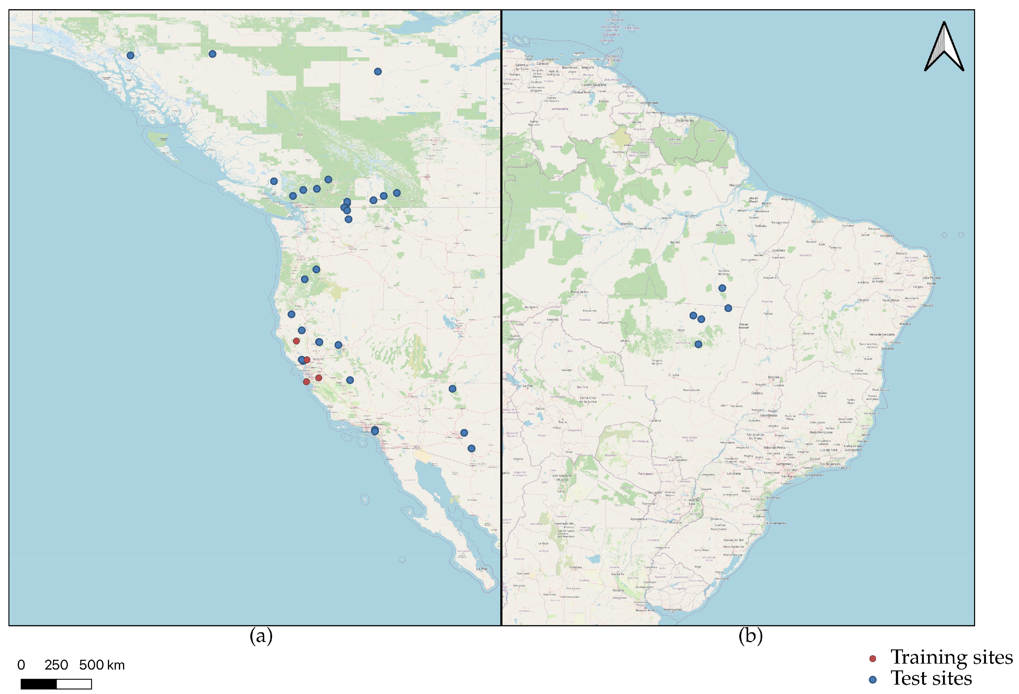
2.1. Study Area
2.2. GOES-R ABI Imagery
2.3. VIIRS Active Fire Product
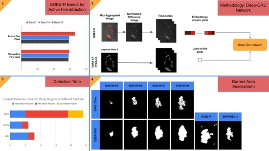
3. Methods
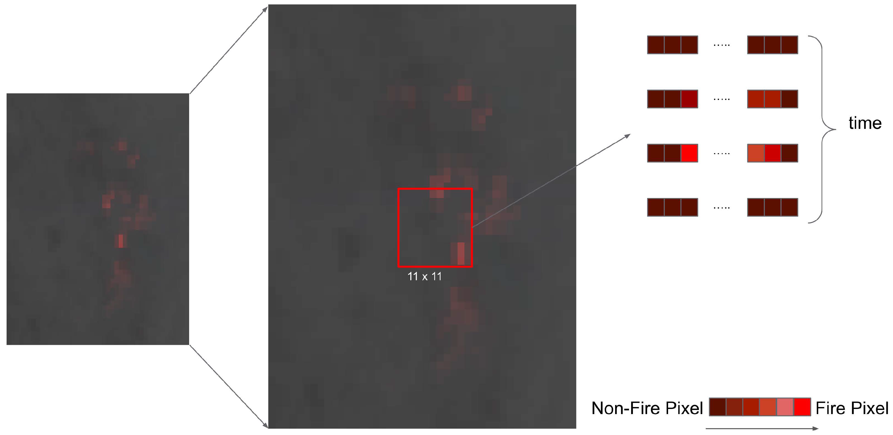
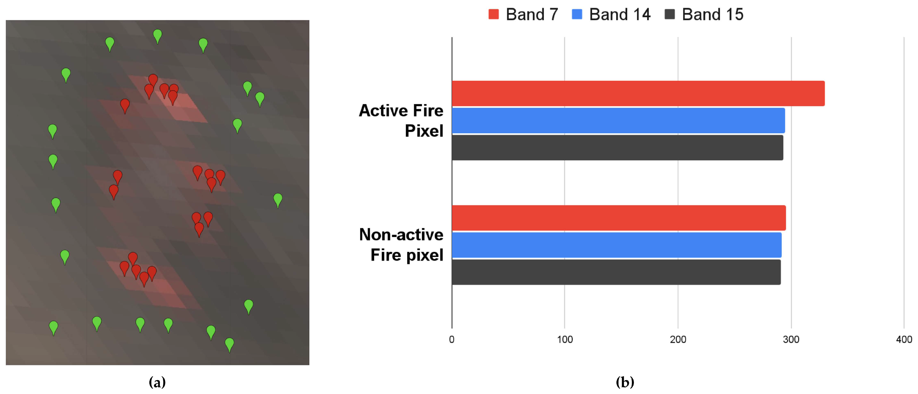
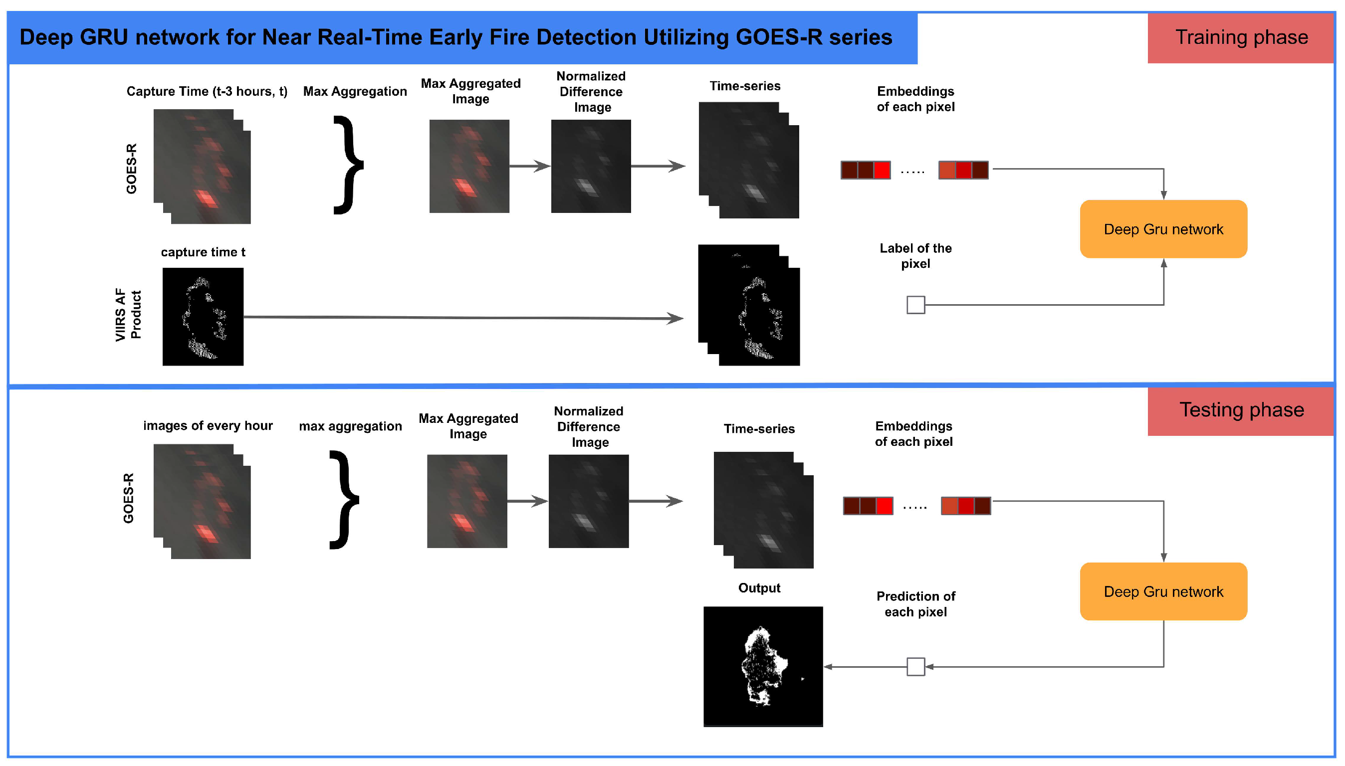
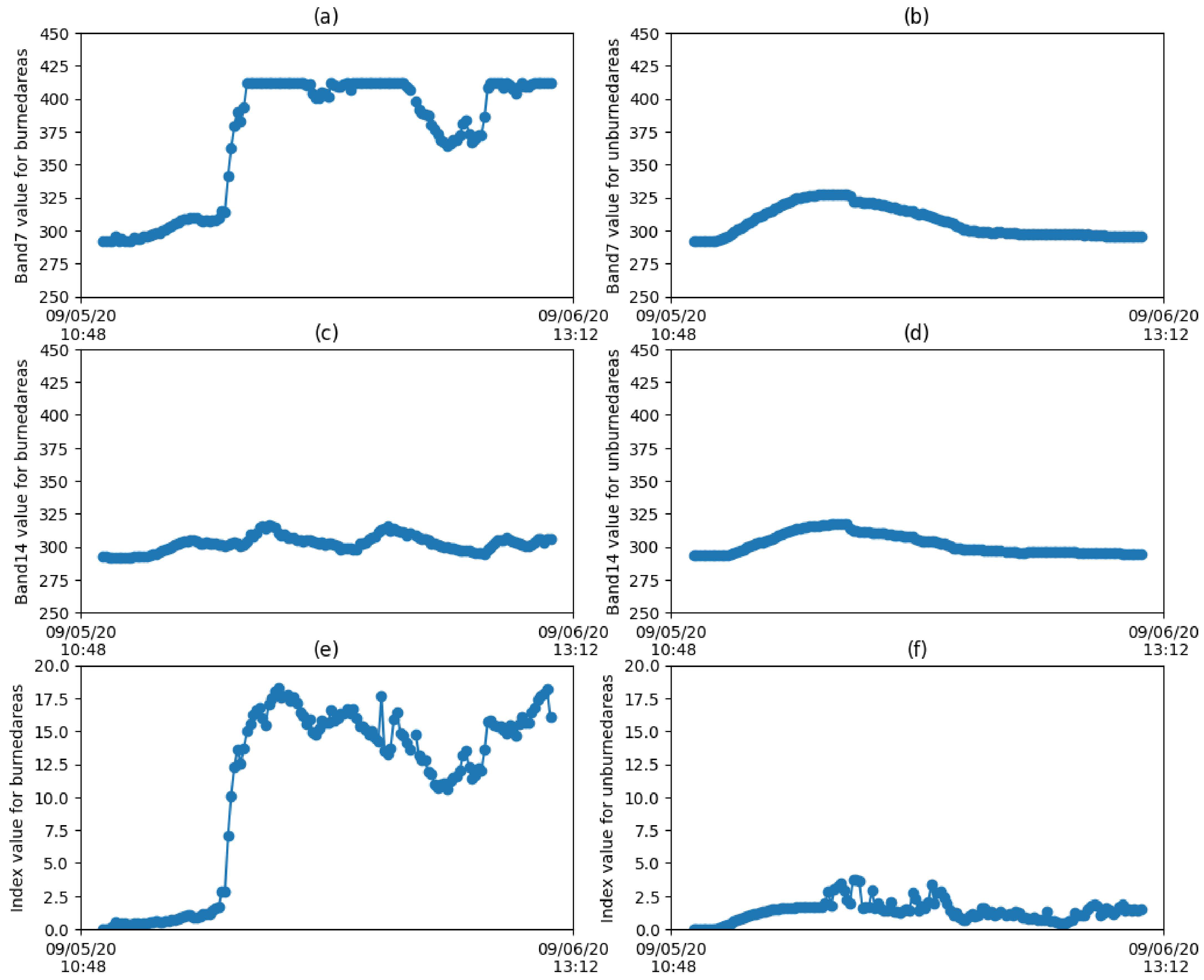
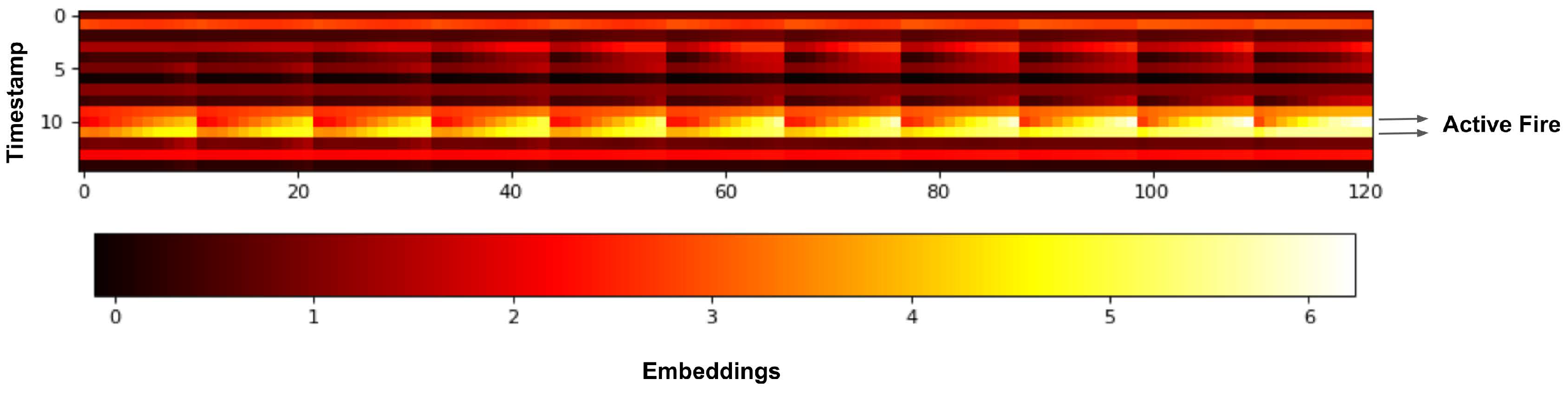
3.1. Dataset Generation and Preprocessing
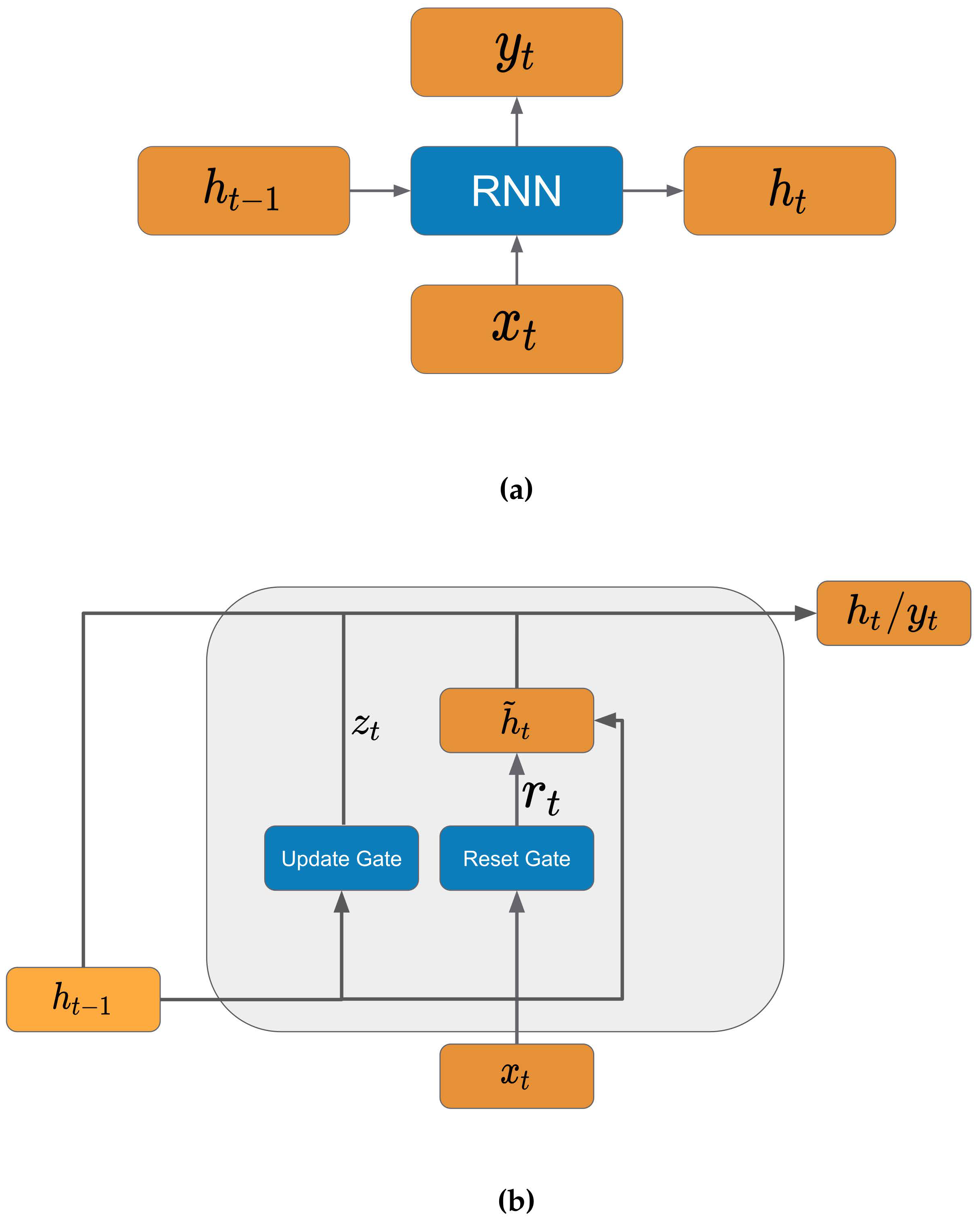
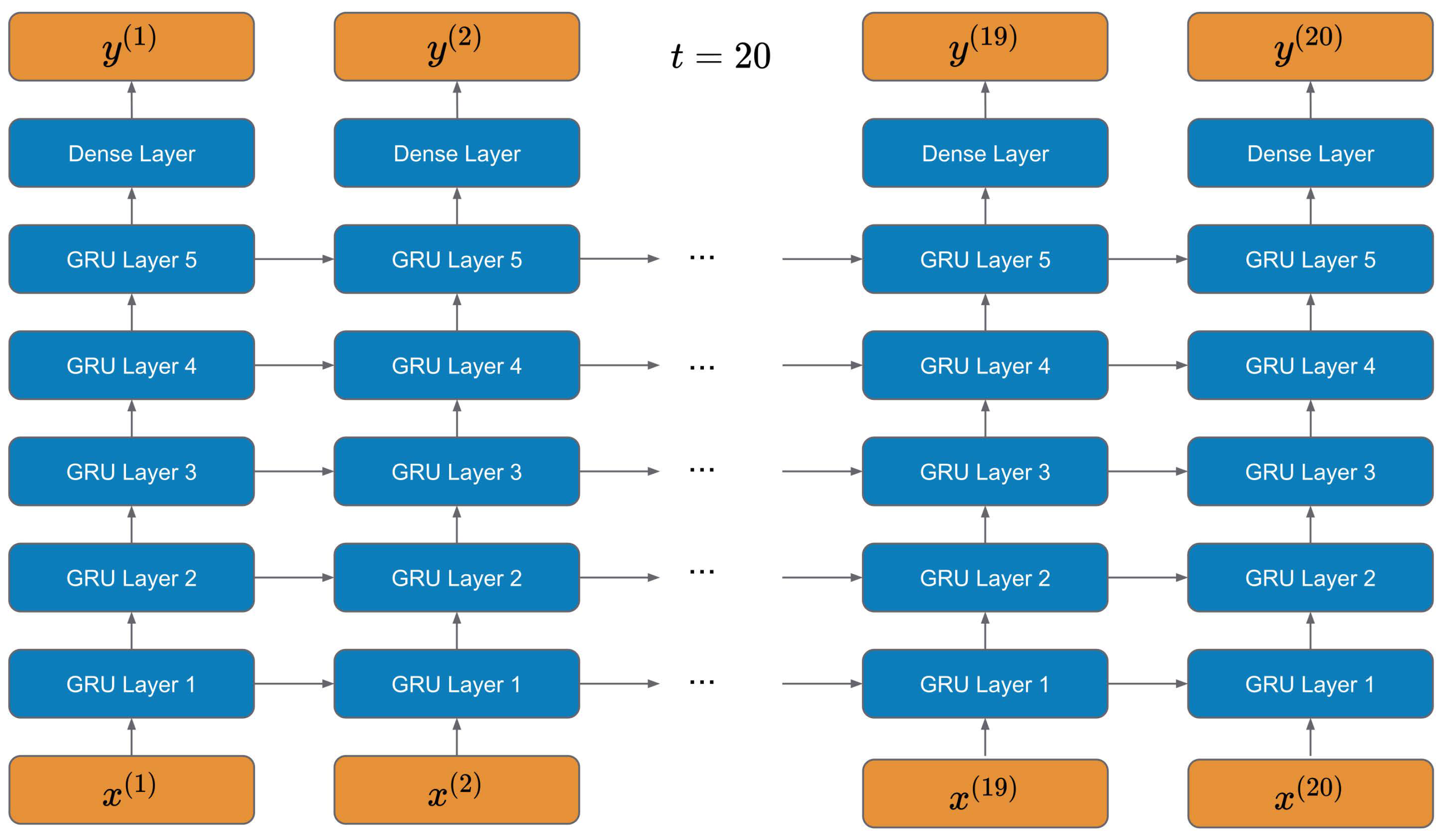
3.2. Deep GRU Network
3.2.1. Gated Recurrent Unit
3.2.2. Deep GRU Network
3.2.3. Loss Function
3.3. Testing Stage
Preprocessing and Inferencing
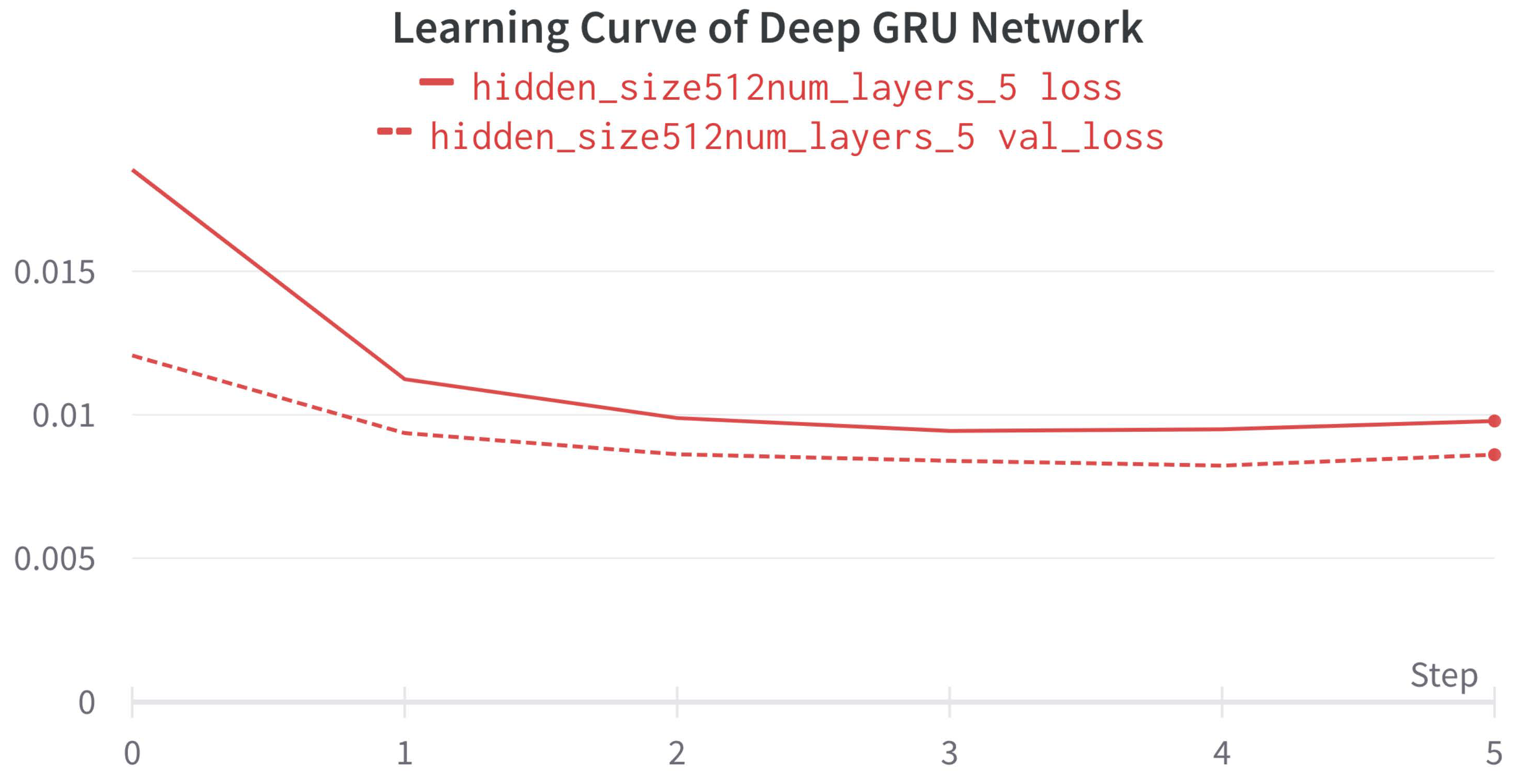
3.4. Setup
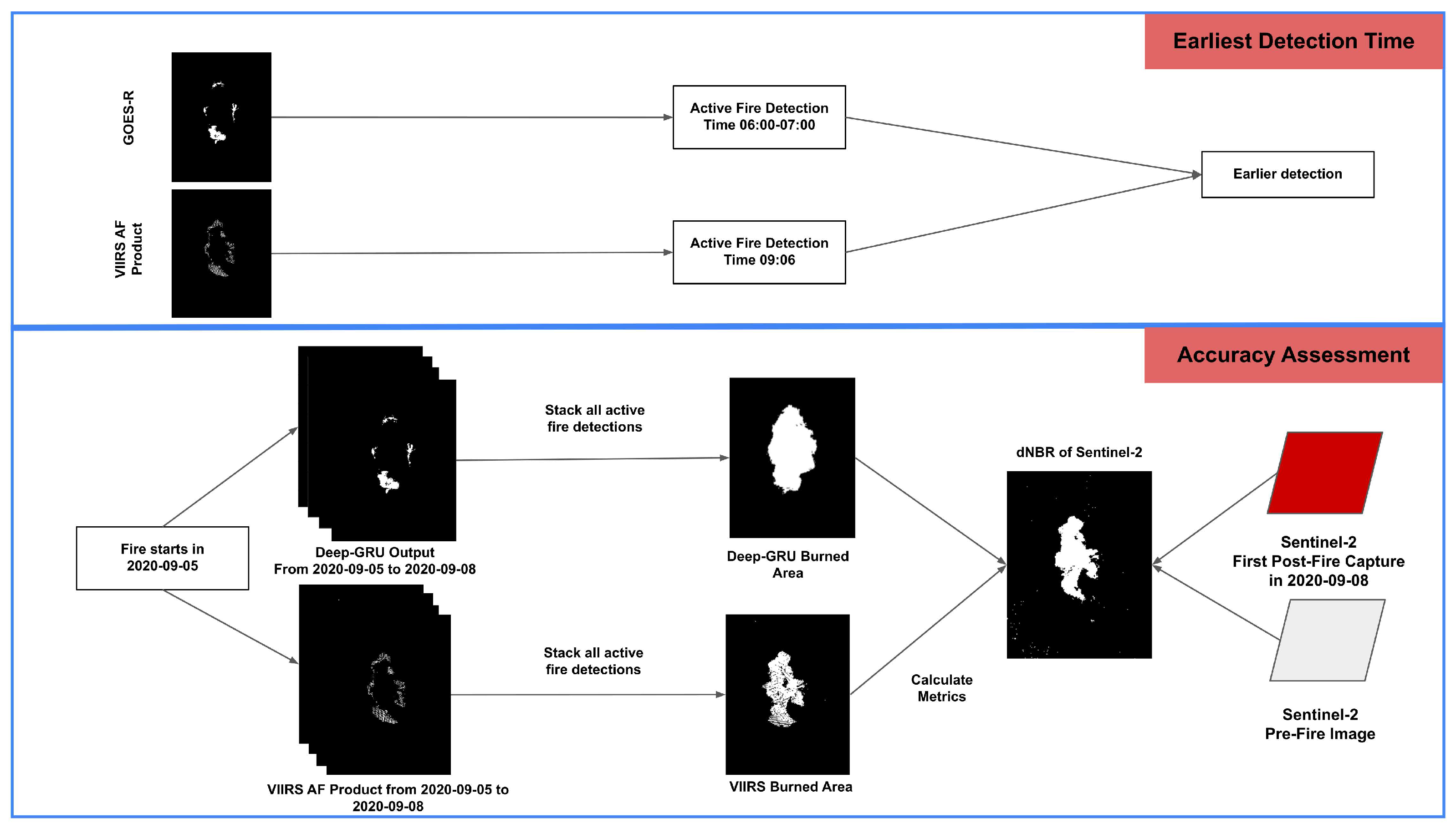
3.5. Accuracy Assessment
4. Results
4.1. Earliest Detection of Active Fires
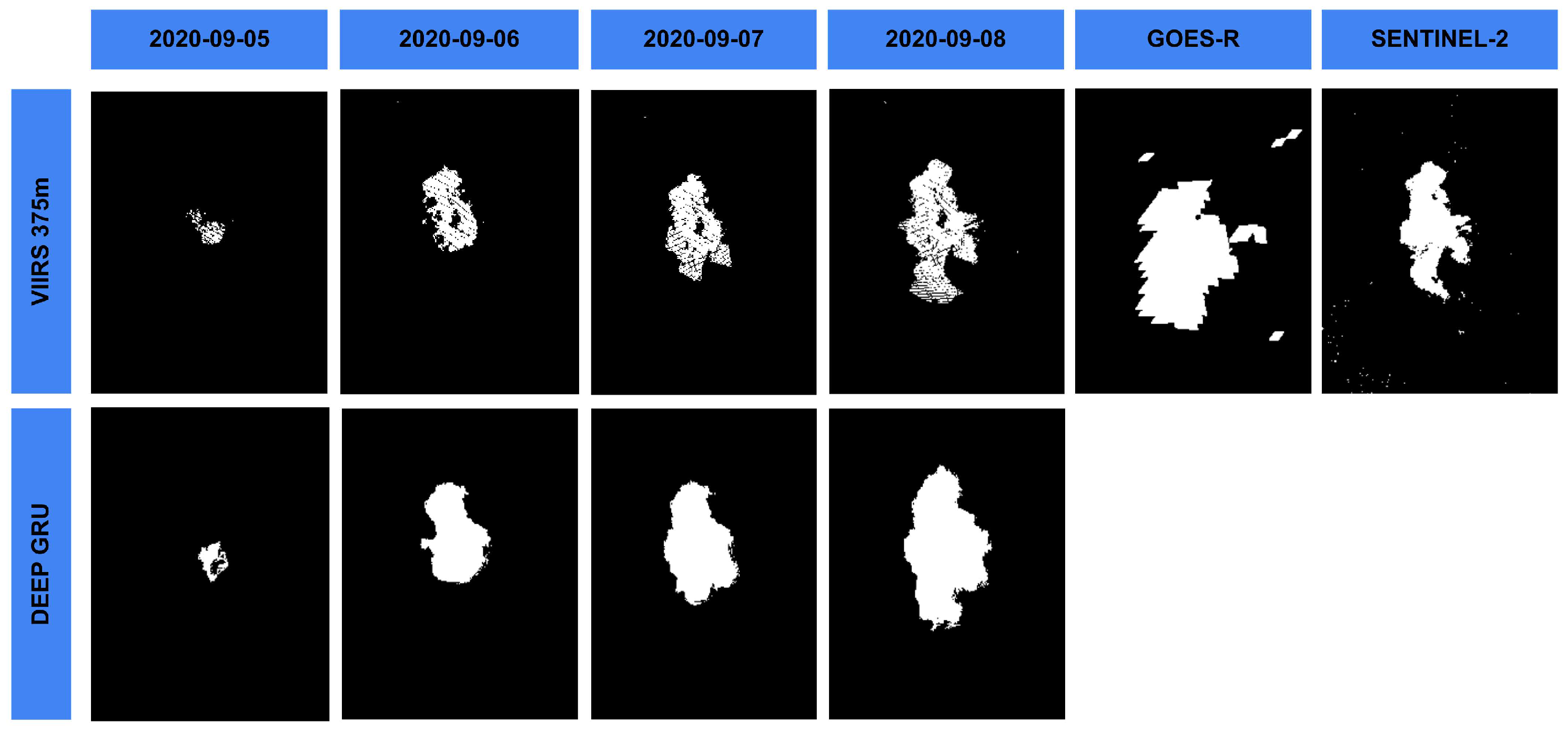
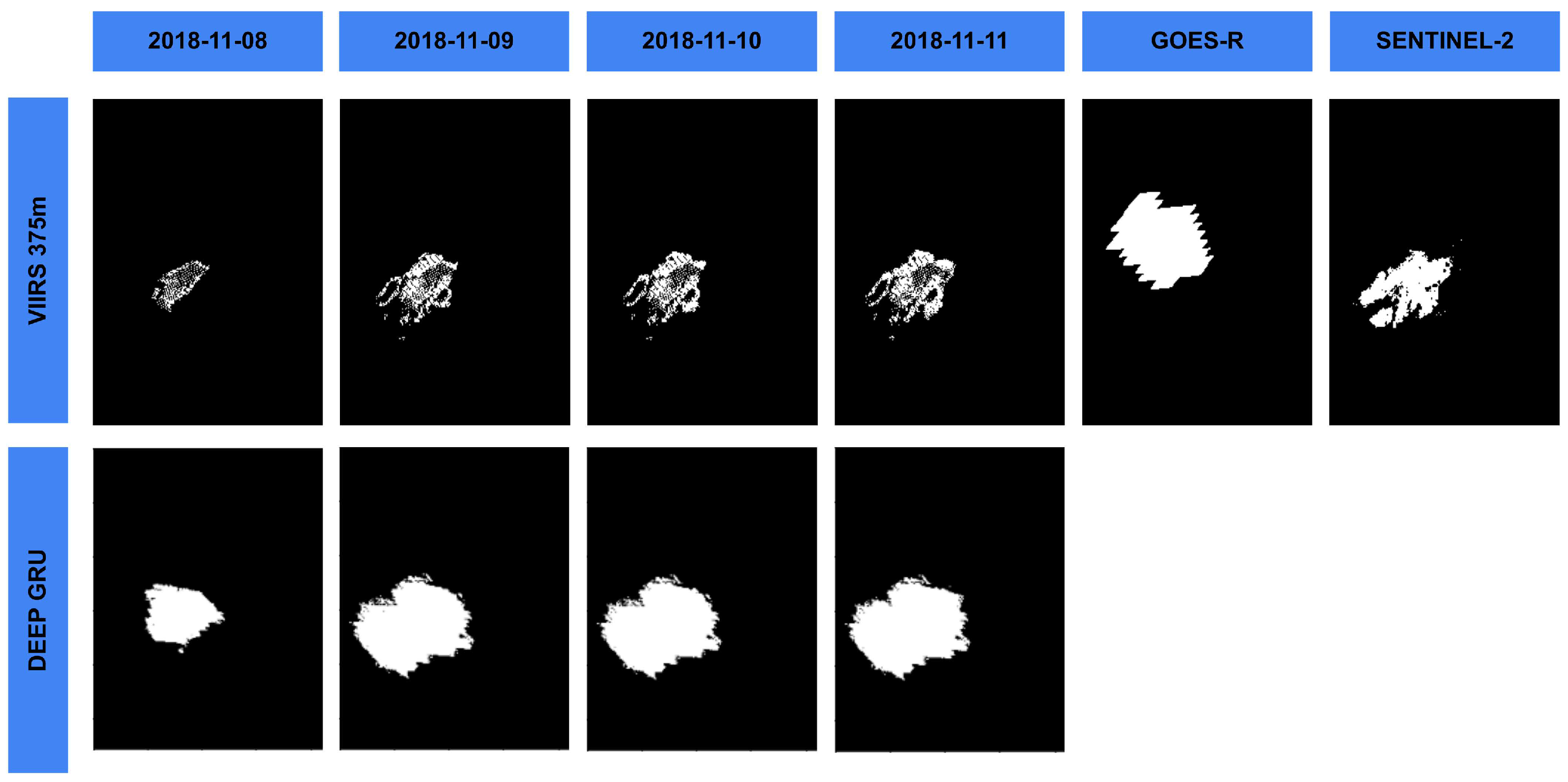
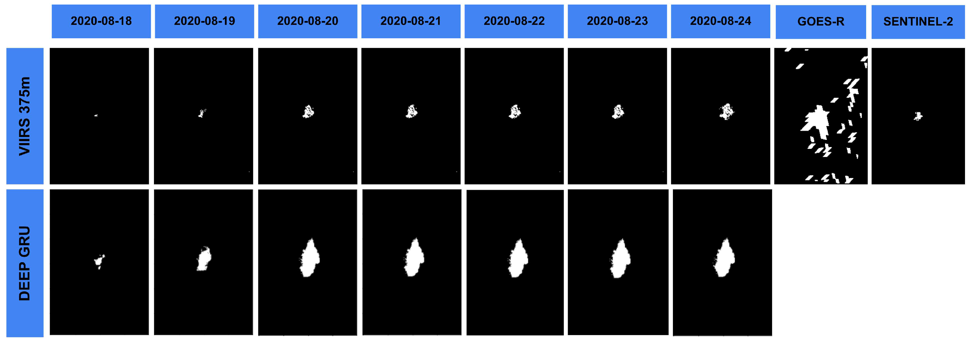
4.2. Accuracy Assessment on Burned Areas
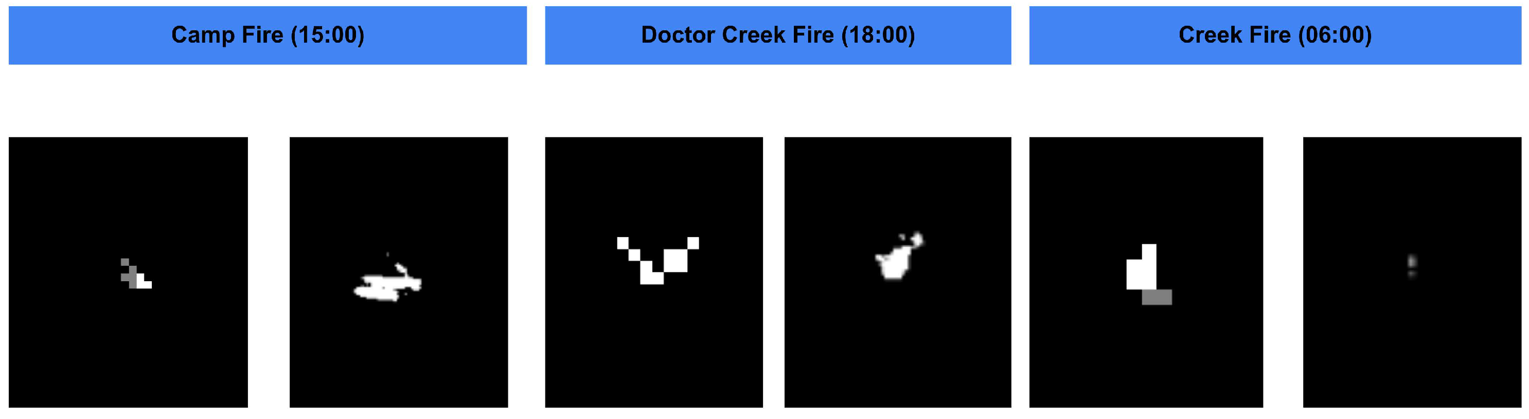
4.2.1. The Creek Fire, California, US
4.2.2. The Camp Fire, California, US
4.2.3. The Doctor Creek Fire, British Columbia, Canada
5. Discussion
5.1. Earliest Detection of Active Fires
5.2. Accuracy Assessment on Burned Areas
6. Conclusions
- The proposed network leverage GOES-R time-series and is possible to detect majorities of the wildfire in study areas earlier than the wildly used VIIRS Active Fire Product in NASA’s Fire Information for Resource Management System. The study areas spread across low-latitude regions mid-latitude regions and high-latitude regions. It shows good generalizability in detecting wildfires in the early stage.
- The proposed method provides good indication of areas affected by the wildfires in the early stage for low-resolution and mid-resolution regions compared to GOES-R Active Fire product. Especially, it significantly reduced the false alarms of GOES-R Active Fire product. For high-latitude regions such as Doctor Creek Fire in British Columbia, the detection shows high error of commission because of the distortion caused by the terminologies of geostationary satellites. Also, for the first detection of the active fire, the proposed method also shows more accurate location of the wildfire compared to GOES-R Active Fire product, while VIIRS active fire product is not available at that time.
Author Contributions
Funding
Data Availability Statement
Conflicts of Interest
Sample Availability
Abbreviations
| EO | Earth Observation |
| DL | Deep Learning |
| GRU | Gated Recurrent Neural Network |
| LSTM | Long Short-Term Memory |
| GOES-R | Geostationary Operational Environmental Satellites R Series |
| SLSTR | Sea and Land Surface Temperature Radiometer |
| VIIRS | Visible Infrared Imaging Radiometer Suite |
| MODIS | Moderate Resolution Imaging Spectroradiometer |
References
- Canadell, J.G.; Monteiro, P.M.; Costa, M.H.; Da Cunha, L.C.; Cox, P.M.; Alexey, V.; Henson, S.; Ishii, M.; Jaccard, S.; Koven, C.; et al. Global carbon and other biogeochemical cycles and feedbacks. In Proceedings of the AGU Fall Meeting, Online, 13–17 December 2021. [Google Scholar]
- Pradhan, B.; Suliman, M.; Awang, M.A.B. Forest fire susceptibility and risk mapping using remote sensing and geographical information systems (GIS). Disaster Prev. Manag. 2007, 16, 344–352. [Google Scholar] [CrossRef]
- San-Miguel-Ayanz, J.; Ravail, N. Active Fire Detection for Fire Emergency Management: Potential and Limitations for the Operational Use of Remote Sensing. Nat. Hazards 2005, 35, 361–376. [Google Scholar] [CrossRef]
- Hu, X.; Ban, Y.; Nascetti, A. Sentinel-2 MSI data for active fire detection in major fire-prone biomes: A multi-criteria approach. Int. J. Appl. Earth Obs. Geoinf. 2021, 101, 102347. [Google Scholar] [CrossRef]
- Schroeder, W.; Oliva, P.; Giglio, L.; Quayle, B.; Lorenz, E.; Morelli, F. Active fire detection using Landsat-8/OLI data. Remote Sens. Environ. 2016, 185, 210–220. [Google Scholar] [CrossRef]
- Kumar, S.S.; Roy, D.P. Global operational land imager Landsat-8 reflectance-based active fire detection algorithm. Int. J. Digit. Earth 2018, 11, 154–178. [Google Scholar] [CrossRef]
- Schroeder, W.; Oliva, P.; Giglio, L.; Csiszar, I. The New VIIRS 375 m active fire detection data product: Algorithm description and initial assessment. Remote Sens. Environ. 2014, 143, 85–96. [Google Scholar] [CrossRef]
- Giglio, L.; Schroeder, W.; Justice, C. The collection 6 MODIS active fire detection algorithm and fire products. Remote Sens. Environ. 2016, 178, 31–41. [Google Scholar] [CrossRef]
- Xu, W.; Wooster, M.; He, J.; Zhang, T. First study of Sentinel-3 SLSTR active fire detection and FRP retrieval: Night-time algorithm enhancements and global intercomparison to MODIS and VIIRS AF products. Remote Sens. Environ. 2020, 248, 111947. [Google Scholar] [CrossRef]
- Oliva, P.; Schroeder, W. Assessment of VIIRS 375 m active fire detection product for direct burned area mapping. Remote Sens. Environ. 2015, 160, 144–155. [Google Scholar] [CrossRef]
- Schroeder, W.; Prins, E.; Giglio, L.; Csiszar, I.; Schmidt, C.; Morisette, J.; Morton, D. Validation of GOES and MODIS active fire detection products using ASTER and ETM+ data. Remote Sens. Environ. 2008, 112, 2711–2726. [Google Scholar] [CrossRef]
- Li, F.; Zhang, X.; Kondragunta, S. Biomass Burning in Africa: An Investigation of Fire Radiative Power Missed by MODIS Using the 375 m VIIRS Active Fire Product. Remote. Sens. 2020, 12, 1561. [Google Scholar]
- Fu, Y.; Li, R.; Wang, X.; Bergeron, Y.; Valeria, O.; Chavardès, R.D.; Wang, Y.; Hu, J. Fire Detection and Fire Radiative Power in Forests and Low-Biomass Lands in Northeast Asia: MODIS versus VIIRS Fire Products. Remote. Sens. 2020, 12, 2870. [Google Scholar] [CrossRef]
- Koltunov, A.; Ustin, S.; Quayle, B.; Schwind, B. Early Fire Detection (GOES-EFD) System Prototype. In Proceedings of the ASPRS Annual Conference, Sacramento, CA, USA, 19–23 March 2012. [Google Scholar]
- Koltunov, A.; Ustin, S.L.; Quayle, B.; Schwind, B.; Ambrosia, V.; Li, W. The development and first validation of the GOES Early Fire Detection (GOES-EFD) algorithm. Remote Sens. Environ. 2016, 184, 436–453. [Google Scholar]
- Kotroni, V.; Cartalis, C.; Michaelides, S.; Stoyanova, J.; Tymvios, F.; Bezes, A.; Christoudias, T.; Dafis, S.; Giannakopoulos, C.; Giannaros, T.M.; et al. DISARM Early Warning System for Wildfires in the Eastern Mediterranean. Sustainability 2020, 12, 6670. [Google Scholar] [CrossRef]
- Schmidt, C.; Hoffman, J.; Prins, E.; Lindstrom, S. GOES-R Advanced Baseline Imager (ABI) Algorithm Theoretical Basis Document for Fire/Hot Spot Characterization; Version 2.0; NOAA: Silver Spring, MD, USA, 2010.
- Li, F.; Zhang, X.; Kondragunta, S.; Schmidt, C.C.; Holmes, C.D. A preliminary evaluation of GOES-16 active fire product using Landsat-8 and VIIRS active fire data, and ground-based prescribed fire records. Remote Sens. Environ. 2020, 237, 111600. [Google Scholar]
- Hall, J.V.; Zhang, R.; Schroeder, W.; Huang, C.; Giglio, L. Validation of GOES-16 ABI and MSG SEVIRI active fire products. Int. J. Appl. Earth Obs. Geoinf. 2019, 83, 101928. [Google Scholar] [CrossRef]
- Zhu, X.; Tuia, D.; Mou, L.; Xia, G.S.; Zhang, L.; Xu, F.; Fraundorfer, F. Deep learning in remote sensing: A review. arXiv 2017, arXiv:1710.03959. [Google Scholar]
- Ban, Y.; Zhang, P.; Nascetti, A.; Bevington, A.R.; Wulder, M. Near Real-Time Wildfire Progression Monitoring with Sentinel-1 SAR Time Series and Deep Learning. Sci. Rep. 2020, 10, 1322. [Google Scholar]
- Mou, L.; Ghamisi, P.; Zhu, X.X. Deep Recurrent Neural Networks for Hyperspectral Image Classification. IEEE Trans. Geosci. Remote Sens. 2017, 55, 3639–3655. [Google Scholar] [CrossRef]
- Toan, N.T.; Phan, T.C.; Hung, N.; Jo, J. A deep learning approach for early wildfire detection from hyperspectral satellite images. In Proceedings of the 7th International Conference on Robot Intelligence Technology and Applications (RiTA), Daejeon, Korea, 1–3 November 2019; pp. 38–45. [Google Scholar]
- Cho, K.; Merrienboer, B.V.; Çaglar, G.; Bahdanau, D.; Bougares, F.; Schwenk, H.; Bengio, Y. Learning Phrase Representations using RNN Encoder–Decoder for Statistical Machine Translation. arXiv 2014, arXiv:1406.1078. [Google Scholar]
- Mission Overview|GOES-R Series. Available online: https://www.goes-r.gov/mission/mission.html (accessed on 4 July 2021).
- Barducci, A.; Guzzi, D.; Marcoionni, P.; Pippi, I. Comparison of fire temperature retrieved from SWIR and TIR hyperspectral data. Infrared Phys. Technol. 2004, 46, 1–9. [Google Scholar] [CrossRef]
- Gorelick, N.; Hancher, M.; Dixon, M.; Ilyushchenko, S.; Thau, D.; Moore, R. Google Earth Engine: Planetary-scale geospatial analysis for everyone. Remote Sens. Environ. 2017, 202, 18–27. [Google Scholar]
- Hochreiter, S.; Schmidhuber, J. Long Short-Term Memory. Neural Comput. 1997, 9, 1735–1780. [Google Scholar] [PubMed]
- Wang, W.; Yang, N.; Wei, F.; Chang, B.; Zhou, M. Gated Self-Matching Networks for Reading Comprehension and Question Answering. In Proceedings of the 55th Annual Meeting of the Association for Computational Linguistics, Vancouver, BC, Canada, 30 July–4 August 2017. [Google Scholar]
- Lin, T.Y.; Goyal, P.; Girshick, R.B.; He, K.; Dollár, P. Focal Loss for Dense Object Detection. IEEE Trans. Pattern Anal. Mach. Intell. 2020, 42, 318–327. [Google Scholar] [CrossRef] [PubMed] [Green Version]
- Abadi, M.; Barham, P.; Chen, J.; Chen, Z.; Davis, A.; Dean, J.; Devin, M.; Ghemawat, S.; Irving, G.; Isard, M.; et al. TensorFlow: A system for large-scale machine learning. In Proceedings of the 15th USENIX Symposium on Operating Systems Design and Implementation, Savannah, GA, USA, 2–4 November 2016. [Google Scholar]


| Training Sites | ||||||||
|---|---|---|---|---|---|---|---|---|
| Political Location | Longitude | Latitude | Start Date | Fire Name | Landcover | Duration | Climate Zone | Burnt Before |
| California, US | −122.97 | 39.87 | 15 August 2022 | August Complex Fire | Needleleaf Forests Savannas | 86 Days | Subtropical Zone | No |
| −122.28 | 37.09 | 17 August 2022 | CZU Lighting Complex Fire | Needleleaf Forests | 42 Days | Subtropical Zone | No | |
| −122.24 | 38.59 | 16 August 2022 | LNU Lighting Complex Fire | Savannas | 38 Days | Subtropical Zone | Yes, 2018 | |
| −121.44 | 37.35 | 18 August 2022 | SCU Lighting Complex Fire | Shrublands, Savannas | 54 Days | Subtropical Zone | No | |
| Test Sites | |||||||
|---|---|---|---|---|---|---|---|
| Political Location | Longitude | Latitude | Start Date | Fire Name | Landcover | Climate Zone | Burnt Before |
| California, US | −121.42 | 39.81 | 14 July 2021 | Dixie Fire | Needleleaf Forests | Subtropical Zone | No |
| −119.30 | 37.20 | 5 September 2020 | Creek Fire | Savannas | Subtropical Zone | No | |
| −117.68 | 33.88 | 26 October 2020 | Blue Ridge Fire | Shrublands | Subtropical Zone | No | |
| −117.66 | 33.74 | 26 October 2020 | Silverado Fire | Grasslands | Subtropical Zone | No | |
| −117.67 | 33.74 | 2 December 2020 | Bond Fire | Grasslands | Subtropical Zone | No | |
| −122.50 | 38.57 | 27 September 2020 | Glass Fire | Savannas | Subtropical Zone | No | |
| −120.12 | 39.69 | 14 August 2020 | North Complex Fire | Savannas | Subtropical Zone | No | |
| −121.43 | 39.81 | 8 November 2018 | Camp Fire | Savannas | Subtropical Zone | No | |
| −122.63 | 38.61 | 8 October 2017 | Tubbs Fire | Grasslands | Subtropical Zone | No | |
| −122.62 | 40.65 | 23 July 2018 | Carr Fire | Shrublands | Temperate Zone | No | |
| British Columbia Canada | −116.10 | 50.09 | 18 August 2020 | N21257 | Savannas | Temperate Zone | No |
| −117.01 | 49.85 | 17 August 2020 | N51250 | Savannas | Temperate Zone | Yes | |
| −119.54 | 49.36 | 18 August 2020 | N51287 | Savannas | Temperate Zone | No | |
| −123.22 | 49.88 | 15 April 2020 | V30067 | Needleleaf Forests | Temperate Zone | No | |
| −128.70 | 59.55 | 27 May 2019 | R90376 | Savannas | Temperate Zone | No | |
| −119.50 | 49.42 | 5 August 2019 | K51244 | Savannas | Temperate Zone | No | |
| −134.35 | 59.43 | 3 August 2019 | R90881 | Needleleaf Forests, Grasslands | Temperate Zone | No | |
| −119.66 | 49.04 | 13 May 2019 | K50271 | Grasslands | Temperate Zone | No | |
| −119.70 | 49.06 | 26 July 2019 | K51089 | Grasslands | Temperate Zone | No | |
| −117.70 | 49.58 | 19 August 2020 | N71114 | Needleleaf Forests | Temperate Zone | No | |
| −122.50 | 50.20 | 18 August 2020 | V31179 | Needleleaf Forests | Temperate Zone | No | |
| −124.53 | 50.84 | 17 August 2020 | V51227 | Needleleaf Forests | Temperate Zone | No | |
| −121.57 | 50.28 | 29 June 2021 | Lytton Fire | Savannas | Temperate Zone | No | |
| −120.79 | 50.92 | 28 June 2021 | Sparks Lake Fire | Needleleaf Forests, Savannas | Temperate Zone | No | |
| Alberta, Canada | −117.42 | 58.38 | 17 May 2019 | Chuckegg Creek Fire | Savannas | Temperate Zone | No |
| Arizona, US | −111.56 | 33.63 | 13 June 2020 | The Bush Fire | Shrublands, Grasslands | Subtropical Zone | No |
| −112.34 | 36.61 | 8 June 2020 | The Magnum Fire | Shrublands, Grasslands | Subtropical Zone | No | |
| −111.03 | 32.53 | 6 June 2020 | Bighorn Fire | Shrublands | Subtropical Zone | No | |
| Oregon, US | −122.45 | 44.15 | 7 September 2020 | Holiday Farm Fire | Broadleaf Forests | Temperate Zone | No |
| −123.38 | 41.77 | 7 September 2020 | Slater Fire | Needleleaf Foersts, Savannas | Temperate Zone | No | |
| −121.62 | 44.77 | 17 August 2020 | Beachie Creek Fire | Needleleaf Forests | Temperate Zone | No | |
| Amazon, Brazil | −51.61 | −9.894 | 5 September 2020 | brazil_fire_1214 | Broadleaf Forests, Savannas | Tropical Zone | Yes |
| −54.49 | −10.52 | 1 September 2020 | brazil_fire_668 | Broadleaf Forests, Savannas | Tropical Zone | Yes | |
| −53.83 | −10.80 | 31 August 2020 | brazil_fire_675 | Broadleaf Forests | Tropical Zone | Yes | |
| −54.07 | −12.87 | 2 September 2020 | brazil_fire_1341 | Broadleaf Forests | Tropical Zone | Yes | |
| −52.10 | −8.24 | 2 September 2020 | brazil_fire_728 | Broadleaf Forests | Tropical Zone | Yes | |
| Washington State, US | −119.56 | 48.83 | 18 August 2020 | Palmer fire | Grasslands | Temperate Zone | No |
| −119.49 | 48.29 | 7 September 2020 | Cold spring fire | Grasslands | Temperate Zone | No |
| Layers | Layer Type | Input Size | Output Size |
|---|---|---|---|
| Input Layer | Input Layer | N/A | (20, 121) |
| Layer #1 | Dense Layer | (20, 121) | (20, 512) |
| Layer #2 | GRU Layer | (20, 512) | (20, 512) |
| Layer #3 | GRU Layer | (20, 512) | (20, 512) |
| Layer #4 | GRU Layer | (20, 512) | (20, 512) |
| Layer #5 | GRU Layer | (20, 512) | (20, 512) |
| Layer #6 | GRU Layer | (20, 512) | (20, 512) |
| Output Layer | Dense Layer | (20, 512) | (20, 2) |
| Location | Fires | Start Date | Location | FIRMS Time | GOES Time | Result |
|---|---|---|---|---|---|---|
| California, US | Creek fire | 5 September 2020 | (−119.30, 37.20) | 09:06 | 06:00–07:00 | Earlier |
| Blue Ridge Fire | 26 October 2020 | (−117.68, 33.88) | 09:06 | 06:00–07:00 | Earlier | |
| Silverado Fire | 26 October 2020 | (−117.66, 33.74) | 07:54 | 06:00–06:59 | Earlier | |
| Bond Fire | 2 December 2020 | (−117.67, 33.74) | 09:12 | 08:00–09:00 | Earlier | |
| Glass Fire | 27 September 2020 | (−122.50, 38.57) | 21:06 | 11:00–12:00 | Earlier | |
| North Complex Fire | 14 August 2020 | (−120.12, 39.69) | 05:47 +1 day | 20:00–21:00 | Earlier | |
| Camp Fire | 8 November 2018 | (−121.43, 39.81) | 18:14 | 15:00–16:00 | Earlier | |
| Tubbs Fire | 8 October 2017 | (−122.63, 38.61) | 06:32 | 05:00–06:00 | Earlier | |
| Carr Fire | 23 July 2018 | (−122.62, 40.65) | 21:08 | 21:00–22:00 | Similar | |
| Dixie Fire | 14 July 2021 | (−121.42, 39.81) | 20:30 | 05:00–06:00 | Earlier | |
| British Columbia, Canada | N21257 | 18 August 2020 | (−116.10, 50.09) | 20:18 | 18:00–19:00 | Earlier |
| N51250 | 17 August 2020 | (−117.01, 49.85) | 20:42 | 22:00–23:00 | Later | |
| N51287 | 18 August 2020 | (−119.54, 49.36) | 22:00 | 22:00–23:00 | Similar | |
| V30067 | 15 April 2020 | (−123.22, 49.88) | 11:01 | 00:00–01:00 | Earlier | |
| R90376 | 27 May 2019 | (−128.70, 59.55) | 22:26 | 22:00–23:00 | Similar | |
| K51244 | 5 August 2019 | (−119.50, 49.42) | 20:30 | 19:00–20:00 | Earlier | |
| R90881 | 3 August 2019 | (−134.35, 59.43) | 22:52 | 22:00–23:00 | Similar | |
| K50271 | 13 May 2019 | (−119.66, 49.04) | 10:06 | 20:00–21:00 | Earlier | |
| K51089 | 26 July 2019 | (−119.70, 49.06) | 21:58 | 01:00–02:00 +1 day | Later | |
| N71114 | 19 August 2020 | (−117.70, 49.58) | 08:36 | 01:00–02::00 | Earlier | |
| V31179 | 18 August 2020 | (−122.50, 50.20) | 08:54 | 18:00–19:00 | Later | |
| V51227 | 17 August 2020 | (−124.53, 50.84) | 20:45 | 20:00–21:00 | Similar | |
| Lytton Fire | 29 June 2021 | (−121.57, 50.28) | 10:30 | 22:00–23:00 | Later | |
| Sparks Lake Fire | 28 June 2021 | (−120.79, 50.92) | 21:54 | 00:00–01:00 +1 day | Later | |
| Alberta, Canada | Chuckegg Creek Fire | 17 May 2019 | (−117.42, 58.38) | 08:59 | 21:00–22:00 | Later |
| Arizona State, US | The bush fire | 13 June 2020 | (−111.56, 33.63) | 09:18 +1 day | 20:00–20:59 | Earlier |
| The magnum fire | 8 June 2020 | (−112.34, 36.61) | 09:20 +1 day | 22:00–23:00 | Earlier | |
| Bighorn fire | 6 June 2020 | (−111.03, 32.53) | 09:18 | 11:00–12:00 | Later | |
| Oregon State, US | Holiday farm fire | 7 September 2020 | (−122.45, 44.15) | 09:00 | 05:00–06:00 | Earlier |
| Slater fire | 7 September 2020 | (−123.38, 41.77) | 20:24 | 15:00–16:00 | Earlier | |
| Beachie creek fire | 17 August 2020 | (−121.62, 44.77) | 09:12 | 10:00-11:00 | Later | |
| Amazon, Brazil | brazil_fire_1214 | 5 September 2020 | (−51.61, −9.894) | 16:06 | 14:00–15:00 | Earlier |
| brazil_fire_668 | 1 September 2020 | (−54.49, −10.52) | 04:42 | 00:00–01:00 | Earlier | |
| brazil_fire_675 | 31 August 2020 | (−53.83, −10.80) | 05:00 | 00:00–01:00 | Earlier | |
| brazil_fire_1341 | 2 September 2020 | (−54.07, −12.87) | 04:06 | 00:00–01:00 | Earlier | |
| brazil_fire_728 | 2 September 2020 | (−52.10, −8.24) | 17:00 | 14:00–15:00 | Earlier | |
| Washington State, US | Palmer fire | 18 August 2020 | (−119.56, 48.83) | 22:00 | 22:00–23:00 | Similar |
| Cold spring fire | 7 September 2020 | (−119.49, 48.29) | 11:00 | 06:00–07:00 | Earlier |
| Study Area | VIIRS 375 m Active Fire Product | GOES-R Active Fire Product | Deep GRU Output | SVM | Random Forest |
|---|---|---|---|---|---|
| Error of Omission | |||||
| Creek Fire | 14.71% | 13.83% | 0.81% | 0.57% | 0.66% |
| Camp Fire | 49.51% | 61.36% | 0.40% | 0.37% | 1.85% |
| Doctor Creek Fire | 16.93% | 0% | 0% | 0% | 0% |
| Error of Comission | |||||
| Creek Fire | 15.96% | 60.02% | 44.41% | 54.38% | 47.07% |
| Camp Fire | 18.34% | 78.97% | 53.57% | 60.41% | 51.57% |
| Doctor Creek Fire | 43.32% | 96.76% | 89.86% | 93.76% | 90.98% |
| F1 Score | |||||
| Creek Fire | 0.8466 | 0.5462 | 0.7125 | 0.6255 | 0.6906 |
| Camp Fire | 0.6239 | 0.2724 | 0.6333 | 0.5667 | 0.6486 |
| Doctor Creek Fire | 0.6738 | 0.0629 | 0.1841 | 0.1174 | 0.1654 |
| Intersection Over Union (IoU) | |||||
| Creek Fire | 0.7340 | 0.3757 | 0.5534 | 0.4550 | 0.5274 |
| Camp Fire | 0.4534 | 0.1576 | 0.4634 | 0.3954 | 0.4799 |
| Doctor Creek Fire | 0.5081 | 0.0324 | 0.1014 | 0.0624 | 0.0901 |
| Hyperparamters | |
|---|---|
| Random Forest | n_estimators = 1000, max_features = ‘auto’, min_sample_split = 2 max_depth = 50, max_leaf_nodes = None min_samples_leaf = 1, max_sample = None, criterion = ‘gini’ |
| SVM | regularization = 1000, gamma = ‘scale’, kernel = ‘rbf’ |
Publisher’s Note: MDPI stays neutral with regard to jurisdictional claims in published maps and institutional affiliations. |
© 2022 by the authors. Licensee MDPI, Basel, Switzerland. This article is an open access article distributed under the terms and conditions of the Creative Commons Attribution (CC BY) license (https://creativecommons.org/licenses/by/4.0/).
Share and Cite
Zhao, Y.; Ban, Y. GOES-R Time Series for Early Detection of Wildfires with Deep GRU-Network. Remote Sens. 2022, 14, 4347. https://doi.org/10.3390/rs14174347
Zhao Y, Ban Y. GOES-R Time Series for Early Detection of Wildfires with Deep GRU-Network. Remote Sensing. 2022; 14(17):4347. https://doi.org/10.3390/rs14174347
Chicago/Turabian StyleZhao, Yu, and Yifang Ban. 2022. "GOES-R Time Series for Early Detection of Wildfires with Deep GRU-Network" Remote Sensing 14, no. 17: 4347. https://doi.org/10.3390/rs14174347
APA StyleZhao, Y., & Ban, Y. (2022). GOES-R Time Series for Early Detection of Wildfires with Deep GRU-Network. Remote Sensing, 14(17), 4347. https://doi.org/10.3390/rs14174347