Optimization of Numerical Methods for Transforming UTM Plane Coordinates to Lambert Plane Coordinates

Abstract

The rapid transformation from UTM (Universal Transverse Mecator) projection to Lambert projection helps to realize timely merging, inversion, and analysis of high-frequency partitioned remote sensing images. In this study, the transformation error and the efficiency of the linear rule approximation method, the improved linear rule approximation method, the hyperbolic transformation method, and the conformal transformation method were compared in transforming the coordinates of sample points on WGS84 (The World Geodetic System 1984)-UTM zonal projections to WGS84-Lambert projection coordinates. The effect of the grid aspect ratio on the coordinate transformation error of the conformal transformation method was examined. In addition, the conformal transformation method-based error spatial pattern of the sample points was analyzed. The results show that the conformal transformation method can better balance error and efficiency than other numerical methods. The error of the conformal transformation method is less affected by grid size. The maximum x-error is less than 0.36 m and the maximum y-error is less than 1.22 m when the grid size reaches 300 km × 300 km. The x- and y-error values decrease when square grids are used; namely, setting the grid aspect ratio close to 1 helps to weaken the effect of increasing grid area on the error. The dispersion of the error distribution and the maximum error of sample points both decrease relative to their minimum distance to the grid edge and stabilize at a minimum distance equal to 70 km. This study can support the rapid integration of massive remote sensing data over large areas.

1. Introduction

In recent years, the rapid growth in the volume of remote sensing data has raised high demands for the performance of spatial data coordinate transformations [1,2,3,4,5,6]. Multisource remote sensing images are generally organized on the WGS1984 (The World Geodetic System 1984)-UTM (Universal Transverse Mecator) projection coordinate system with nonuniform segmentation rules and diverse spatial and temporal resolutions. The rapid transformation of spatial data from the UTM zonal projection coordinate system (applied to the local area) to a conical or cylindrical projection coordinate system (e.g., Lambert projection coordinate system) is important for realizing timely merging, retrieval, and analysis of high-frequency segmented remote sensing images.

Coordinate transformations can be performed by either analytical or numerical methods. Analytical methods have a rigorous foundation of mathematics and require known reference ellipsoid parameters and analytical equations; they are generally more accurate than numerical methods but also more complex and of lower efficiency [7]. Numerical methods use polynomials as approximate functions to transform coordinates; multiple control points are brought into the equations to solve for the coefficients of the polynomial [8]. In general, numerical methods do not require the parameters of the reference ellipsoid and are widely used in scenarios where a high efficiency of coordinate transformation is required [9].

Extensive research on numerical methods for map projection transformation has been carried out. On the one hand, polynomial methods (e.g., binary n-th polynomials; multiplicative polynomials) can be widely used for coordinate transformation between projection coordinate systems with different deformation characteristics [10]. Binary n-th order polynomials are often used for geographic alignment. For example, the field programmable gate array-based optimized second-order polynomial equation developed by Liu et al. [11] was applied to align datasets based on the UTM projection and the State Plane (NAD 27) projection. The results showed that the alignment was eight times faster than PC-based alignment, with an accuracy comparable to that using ENVI [11]. According to the comparative analysis by Bildirici [12] and Ye [13], the multiquadric transform method, hyperbolic transform method, and linear rule approximation method are three polynomial methods with high representativeness and stability. The multiquadric transform model was proposed by Hardy [14] for the representation of terrain and irregular surfaces and has higher efficiency than the traditional summation and power series. Over the following 20 years, the multiquadric method has been used in a wide range of fields, such as geophysics, mapping science and technology, geography, hydrology, and signal processing [15]. The hyperbolic transformation, also known as the bilinear transformation, is a multiplicative polynomial. Zhao et al. [16] applied the hyperbolic transformation method to transform raster maps from Lambert projection to Mercator projection, achieving a good balance between accuracy and efficiency. Bildirici [12] compared the applicability of the multiquadric transformation model with the hyperbolic transformation model for the inverse transformation of equivalent projection and conformal projection coordinate systems. The results suggested that the hyperbolic transformation method has the advantages of higher accuracy and simpler computation than the multiquadric method and that the hyperbolic transformation method has a more uniform error distribution in the conformal projection inverse transformation than the equivalent projection inverse transformation. In the linear rule approximation method [13], linear polynomials are constructed to express the transformation rules between the geographic and projection coordinate systems in the local area and are applied to the forward and inverse transformation between the WGS1984 geographic coordinate system and the WGS1984-UTM projection coordinate system. Experimental results suggested that the accuracy and stability of the linear rule approximation method were higher than those of the hyperbolic transformation method in scenarios where the study area was divided into 0.5′ or 1 km square grids. The linear rule approximation method takes only 0.046 times as long as the truncated series method to perform the transformation of 32,400,000 sample points. The linear rule approximation method was applied by Mu et al. [17] to the scheduling of a large truck fleet based on multilayer matching to meet the computational efficiency requirements of near real-time coordinate transformation.

On the other hand, when the simple polynomial method is used for coordinate transformation, the stability of the error is greatly affected by the distribution of control points [18]. To alleviate this problem, a coordinate transformation scheme between conformal projections based on the theory of complex functions was proposed by Yang [19], Li [20], and Liu [21]. The related typical methods are the conformal polynomial method, difference method, finite element method, and interpolation method [10]. The conformal polynomial algorithm (CT) was proposed by Yang [18] and applied to the transformation of projection coordinates between Gaussian projection zones, which was demonstrated to be more efficient than the traditional transformation formula. Subsequently, the conformal polynomial algorithm was promoted for transformations between different conformal projections and for forward and inverse transformation of conformal projection coordinates, showing low parameter requirements, low error, and high stability [9]. In addition, the implementation of the conformal polynomial method is more flexible and easier than the finite element method and the difference quotient method [20,21].

In addition to the type of polynomial and its method of solving the parameters, the trade-off between coordinate transformation error and efficiency is comprehensively influenced by the local transformation area and the number and distribution of control points [13]. The transformation error generally increases as the area of the transformation region increases. In practice, the study area is split into several subregions by regular rectangular or triangular grids to mitigate error propagation. For each subregion, independent numerical polynomial parameters are fitted by using the grid vertices as control points. The transformation error can be reduced to some extent by decreasing the area of the subregion. When the number of subregions increases to a certain level, the efficiency of the coordinate transformation decreases as the time spent on parameter retrieval increases, and the error stabilizes.

Research on numerical methods and implementation pathways has provided important theoretical and empirical support for this study. However, the applicability of different numerical methods varies with the coordinate transformation scenario, the area, and the shape of the subregion. Which numerical method is more suitable for transforming raster data from UTM zonal projection to Lambert projection? What is the appropriate grid layout scheme? Fewer studies have addressed these questions.

In this study, the linear rule approximation method, the improved linear rule approximation method, the hyperbolic transformation method, and the conformal transformation method were applied to transform the coordinates of the points in the three WGS84-UTM projection zones (i.e., UTM Zone 48N; UTM Zone 50N; UTM Zone 52N) into WGS84-Lambert projection coordinates. For each study area, we mimicked the raster data organization by deploying 33 million uniformly distributed sample points at 200 m intervals. Fifteen square grid segmentation schemes (i.e., 1 × 1; 5 × 5; 10 × 10; 25 × 25; 50 × 50; 75 × 75; 100 × 100; 125 × 125; 150 × 150; 175 × 175; 200 × 200; 225 × 225; 275 × 275; and 300 × 300; unit: km²) were applied to the study area, and then the coordinate transformation errors and efficiency of each numerical method were tested when applying each scheme. The effect of the grid aspect ratio on the error of the conformal transformation method was examined by calculating the coordinate transformation error by setting the grid length in the x-direction to 100, 200, 300, and 400 km and y-direction to 300, 350, 400, 450, 500, 550, and 600 km. In addition, the error distribution pattern of sample points based on the conformal transformation method was analyzed. This study can support the rapid integration of massive remote sensing data in large areas.

The rest of the paper is organized as follows: Section 2 describes in detail the four numerical methods and experimental scenarios involved in this study. Section 3 presents the experimental results of transforming WGS1984 UTM plane coordinates to WGS1984 Lambert plane coordinates using the four numerical methods. Finally, the comparison and application scenarios of the four methods are discussed and summarized in Section 4 and Section 5.

2. Materials and Methods

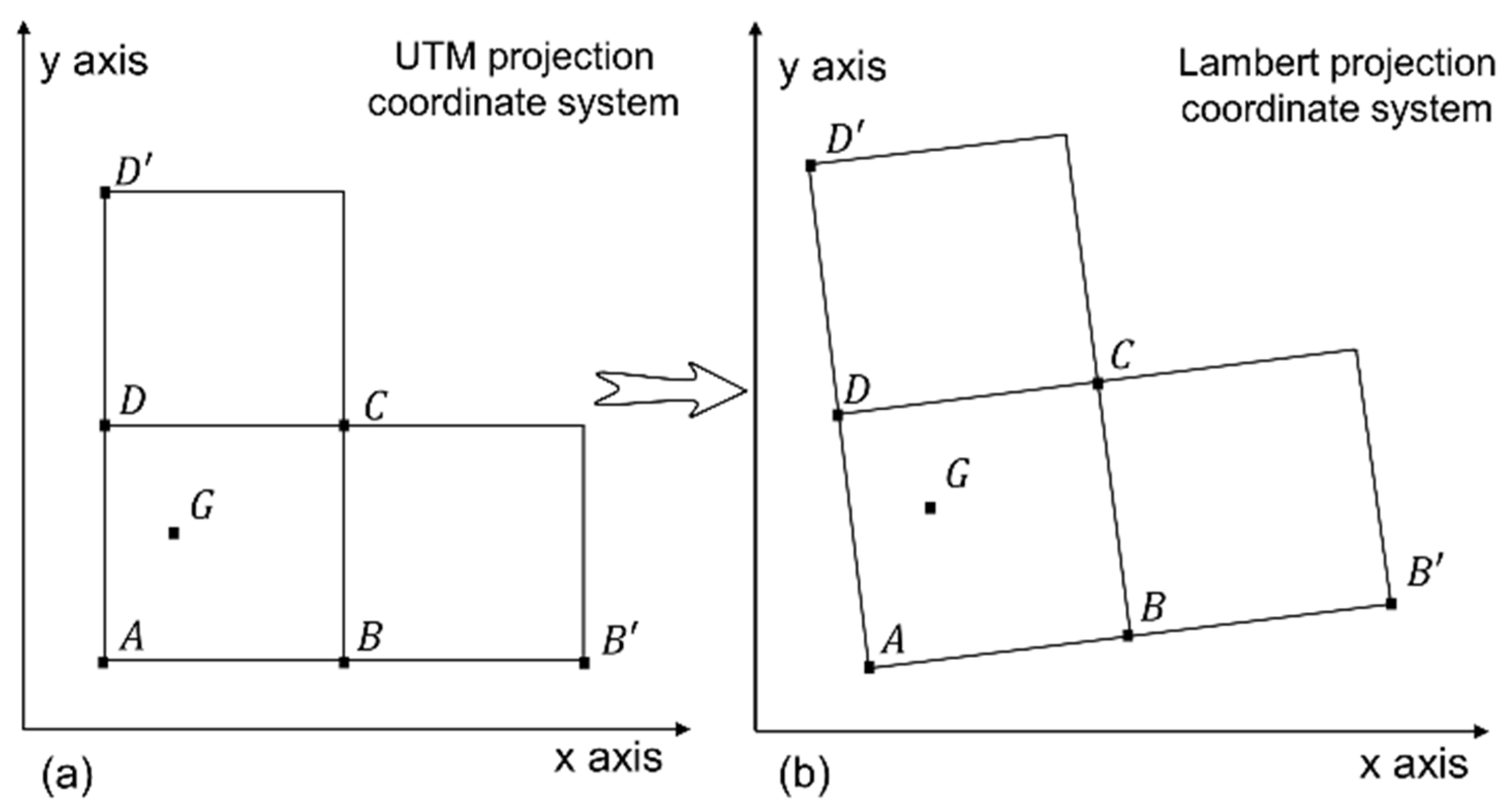
2.1. Numerical Methods

As shown in Figure 1, the four corner points of the rectangular grid are set as A, B, C, and D, and point G is an arbitrary point within the grid. Their coordinates in the WGS84-based UTM projection coordinate system are $\left(x_A,y_A\right),$ $\left(x_B,y_B\right),\left(x_C,y_C\right),\left(x_D,y_D\right),(x_{B\prime },y_{B\prime }),(x_{D\prime },y_{D\prime }),\left(x_G,{\mathrm{y}}_G\right)$, where $x_A=x_D=x_{D\prime },x_B=x_C=x_{B\prime },y_A=y_B=y_{B\prime },y_C=y_D=y_{D\prime }$. Their corresponding coordinates in the Lambert projection coordinate system are $\left(X_A,Y_A\right),$ $\left(X_B,Y_B\right),$ $\left(X_C,Y_C\right),$ $(X_D,Y_D),(X_{B\prime },Y_{B\prime }),(X_{D\prime },Y_{D\prime }),\left(X_G,Y_G\right)$. On this basis, the application of the linear rule approximation method, the improved linear rule approximation method, the hyperbolic transformation method, and the conformal transformation method are illustrated by calculating the coordinates of point G (i.e., $\left(X_G,Y_G\right)$).

2.1.1. Linear Rule Approximation (LRA) Method

The linear rule approximation method equations are listed in Equations (1) and (2).

$$X_G=X_A+m\left(x_G-x_A\right)+n\left(y_G-y_A\right)$$

(1)

$$Y_G=Y_A+p\left(x_G-x_A\right)+q\left(y_G-y_A\right)$$

(2)

where the parameters m, n, p, q are calculated by Equations (3)–(6), $\mathsf{\Delta }x=x_B-x_A$, and $\mathsf{\Delta }y=x_C-y_A$.

$$m=\frac{X_B-X_A}{\mathsf{\Delta }x}$$

(3)

$$n=\frac{X_D-X_A}{\mathsf{\Delta }y}$$

(4)

$$p=\frac{Y_B-Y_A}{\mathsf{\Delta }x}$$

(5)

$$q=\frac{Y_D-Y_A}{\mathsf{\Delta }y}$$

(6)

2.1.2. Improved Linear Rule Approximation (ILRA) Method

The ILRA method adds a correction for deformation in the x- and y-directions based on the LRA method. Its formula is shown in Equations (7) and (8).

$$X_G=X_A+m\left(x_G-x_A\right)+n\left(y_G-y_A\right)+u{(x_G-x_A)}^2+v{(y_G-y_A)}^2$$

(7)

$$Y_G=Y_A+p\left(x_G-x_A\right)+q\left(y_G-y_A\right)+r{(x_G-x_A)}^2+s{(y_G-y_A)}^2$$

(8)

2.1.3. Hyperbolic Transformation (HT) Method

The equation for the HT method is shown in Equations (9) and (10).

$$X_G=a_1{x}_G+a_2{y}_G+a_3{x}_G{y}_G+a_4$$

(9)

$$Y_G=b_1{x}_G+b_2{y}_G+b_3{x}_G{y}_G+b_4$$

(10)

The eight parameters a₁–a₄ and b₁–b₄ can be solved by bringing points A, B, C, and D as control points into the two systems of linear equations, as shown in Equations (11) and (12).

$$\left[\begin{array}{c}{x}_A{y}_A{x}_A{y}_{A}1\\ x_B{y}_B{x}_B{y}_{B}1\\ x_C{y}_C{x}_C{y}_{C}1\\ x_D{y}_D{x}_D{y}_{D}1\end{array}\right]\left[\begin{array}{c}{a}_1\\ a_2\\ a_3\\ a_4\end{array}\right]=\left[\begin{array}{c}{X}_A\\ X_B\\ X_C\\ X_D\end{array}\right]$$

(11)

$$\left[\begin{array}{c}{x}_A{y}_A{x}_A{y}_{A}1\\ x_B{y}_B{x}_B{y}_{B}1\\ x_C{y}_C{x}_C{y}_{C}1\\ x_D{y}_D{x}_D{y}_{D}1\end{array}\right]\left[\begin{array}{c}{b}_1\\ b_2\\ b_3\\ b_4\end{array}\right]=\left[\begin{array}{c}{Y}_A\\ Y_B\\ Y_C\\ Y_D\end{array}\right]$$

(12)

2.1.4. Conformal Transformation (CT) Method

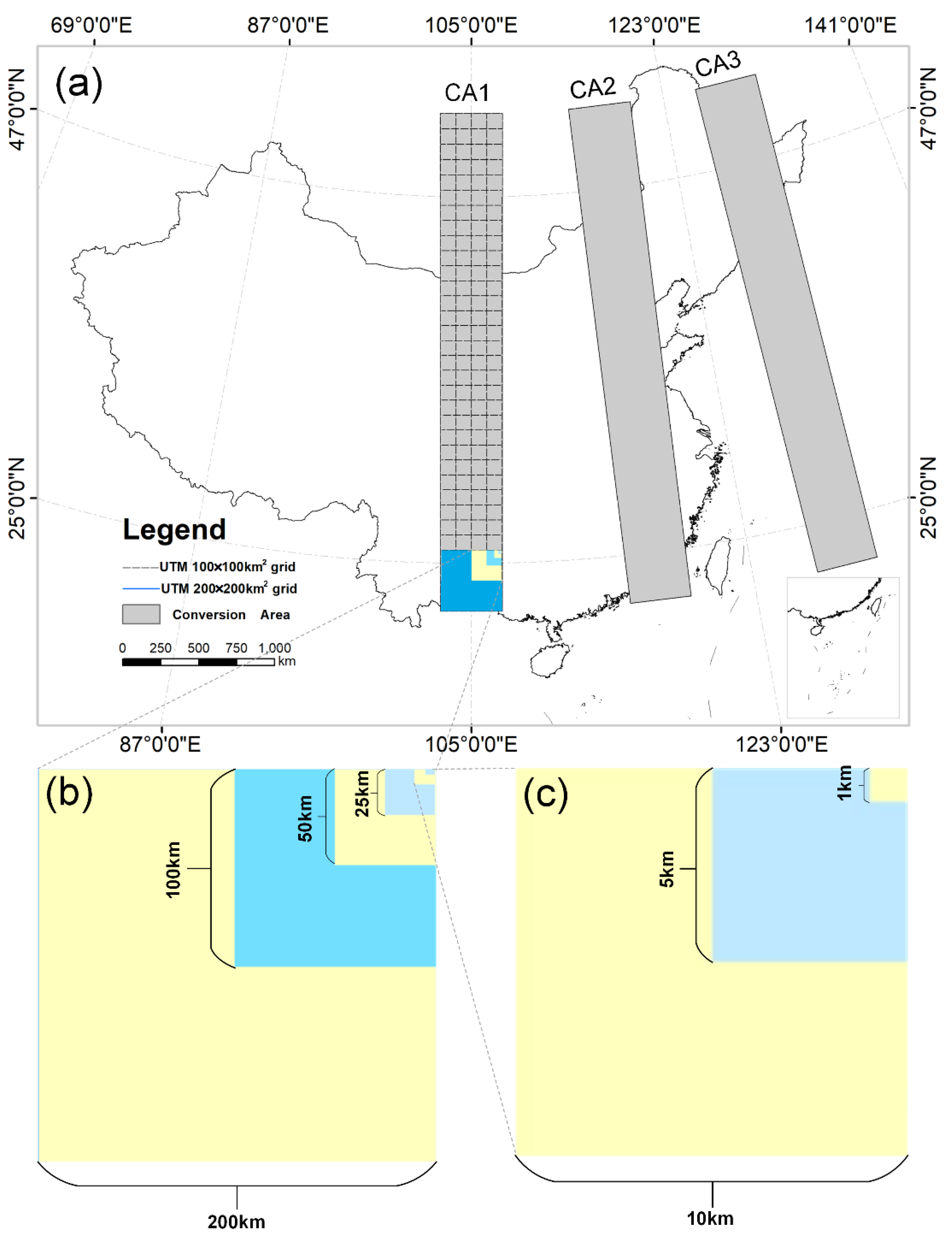
The 3-order conformal polynomial is shown in Equations (13) and (14).

$$X_G=X_A+{\displaystyle \sum }_{i=1}^3(a_i{P}_i-b_i{Q}_i)$$

(13)

$$Y_G=Y_A+{\displaystyle \sum }_{i=1}^3(a_i{Q}_i+b_i{P}_i)$$

(14)

where $Q_i$ and $P_i$ are calculated as shown in Equations (15)–(18).

$$P_1=d_x=x_G-x_A$$

(15)

$$Q_1=d_y=y_G-y_A$$

(16)

$$P_{i+1}=d_x{P}_i-d_y{Q}_i,i=1,2$$

(17)

$$Q_{i+1}=d_y{P}_i+d_x{Q}_i,i=1,2$$

(18)

The six parameters a₁–a₃ and b₁–b₃ can be solved directly by bringing the values of the coordinates of points A, B, C, and D into the system of linear equations in Equation (9) as follows, where the subscript j denotes the number of the three control points and takes values 1, 2, and 3. The three control points are selected as points B, C, and D, in turn. $P_{i1}$ and $Q_{i1}$, $P_{i2}$ and $Q_{i2}$,$\mathrm{and}{P}_{i3}$ and $Q_{i3}$ can be calculated in Equations (19) and (20) by replacing $x_G$ and $y_G$ with $x_B$ and $y_B$, $x_C$ and $y_C$, and $x_D$ and $y_D$, respectively.

$${\displaystyle \sum }_{i=1}^3(a_i{P}_{ij}-b_i{Q}_{ij})=X_j-X_A,j=1,2,3$$

(19)

$${\displaystyle \sum }_{i=1}^3(a_i{Q}_{ij}+b_i{P}_{ij})=Y_j-Y_A,j=1,2,3$$

(20)

2.2. Test Scenarios

In this study, the reference datum for both the UTM projection coordinate system and the Lambert projection coordinate system is the WGS-84 ellipsoid. The projection parameters (

Table 1. Parameters of the Lambert projection system.

Parameter Name	Parameter Value
False easting	0.00°
False northing	0.00°
Central meridian	105.00°E
Standard parallel 1	25.00°N
Standard parallel 2	47.00°N
Scale factor	1.00
Latitude of origin	0.00°

) applicable to China are applied to the Lambert projection coordinate system, whose central meridian longitude is the same as that of UTM Zone 48N. Since the Lambert projection deformation is symmetrical on both sides of the central meridian and is influenced by the distance from the central meridian, the experiments were performed in three projection zones: UTM Zone 48N (90°N–96°N), UTM Zone 50N (102°N–108°N), and UTM Zone 52N (114°N–120°N). For each projection zone, the spatial extent of the study area was designed to be 300–700 km (X-coordinate) and 2450–5750 km (Y-coordinate), as shown in Figure 2. For each study area, 33 million uniformly distributed sample points were deployed at 200 m intervals, mimicking the raster data organization. Fifteen groups of square grids based on row-column ordering (i.e., 1 × 1, 5 × 5, 10 × 10, 25 × 25, 50 × 50, 75 × 75, 100 × 100, 125 × 125, 150 × 150, 175 × 175, 200 × 200, 225 × 225, 275 × 275, and 300 × 300, unit: km²) were applied to divide the entire study area into numerous subareas. On this basis, the linear rule approximation method, improved linear rule approximation method, hyperbolic transformation method, and conformal transformation method were applied to transform the coordinates of the sample points from the UTM projection coordinate system into the Lambert coordinate system. In addition, the coordinate transformation of sample points was implemented as follows:

• In the first step, for a particular numerical method, the four vertices of each subzone are used as control points to calculate their corresponding polynomial parameters. The polynomial parameters are stored in a memory array.
• In the second step, all sample points are grouped according to the spatial extent of the subzone. Sample points within the same subzone are assigned to the same group.
• In the third step, for each group, the polynomial parameters are called from the memory array, and the coordinate transformation is performed in bulk for the sample points belonging to that group.

Another experiment was carried out to test the effect of the grid aspect ratio on the error of the conformal transformation method. A total of 4 × 7 rectangular grid divisions of the study area were designed with lengths of 100, 200, 300, and 400 km in the x-direction and 300, 350, 400, 450, 500, 550, and 600 km in the y-direction.

2.3. Hardware and Software Environment

The hardware and software environment for this study is shown in

Table 2. Experimental software and hardware environment.

Parameter Name	Parameter Value
CPU	AMD Ryzen 7 4700U @ 2.00 GHz (8 cores 8 threads)
Internal storage	16 GB (Micron 8 GB DDR4 3200 MHz × 2)
Operating system	Windows 10 pro 64 bit
Development platform	Microsoft Visual Studio 2019
Programming language	C#

. The results of the projection coordinate transformation based on the map projection library PROJ are considered ‘true values’ and used to calculate the polynomial parameters and coordinate transformation errors for each numerical method.

3. Results

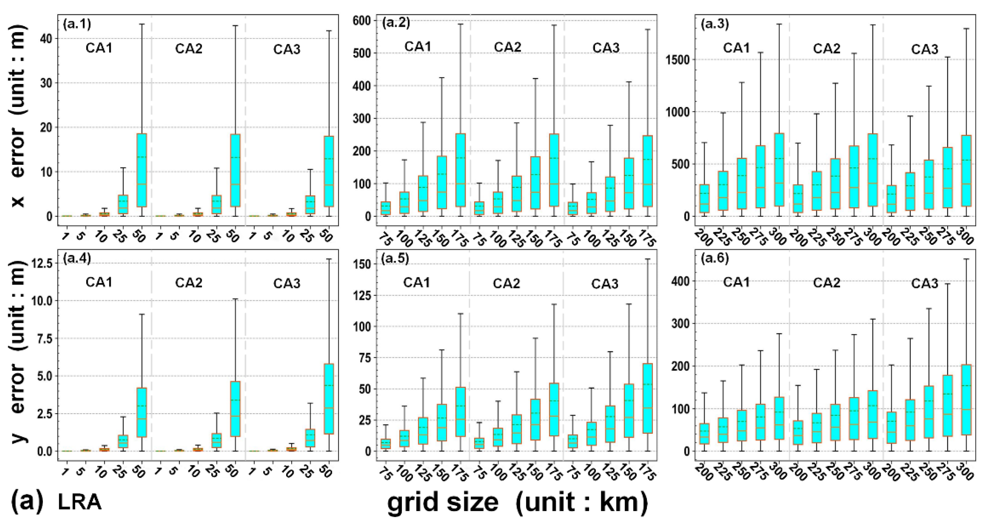
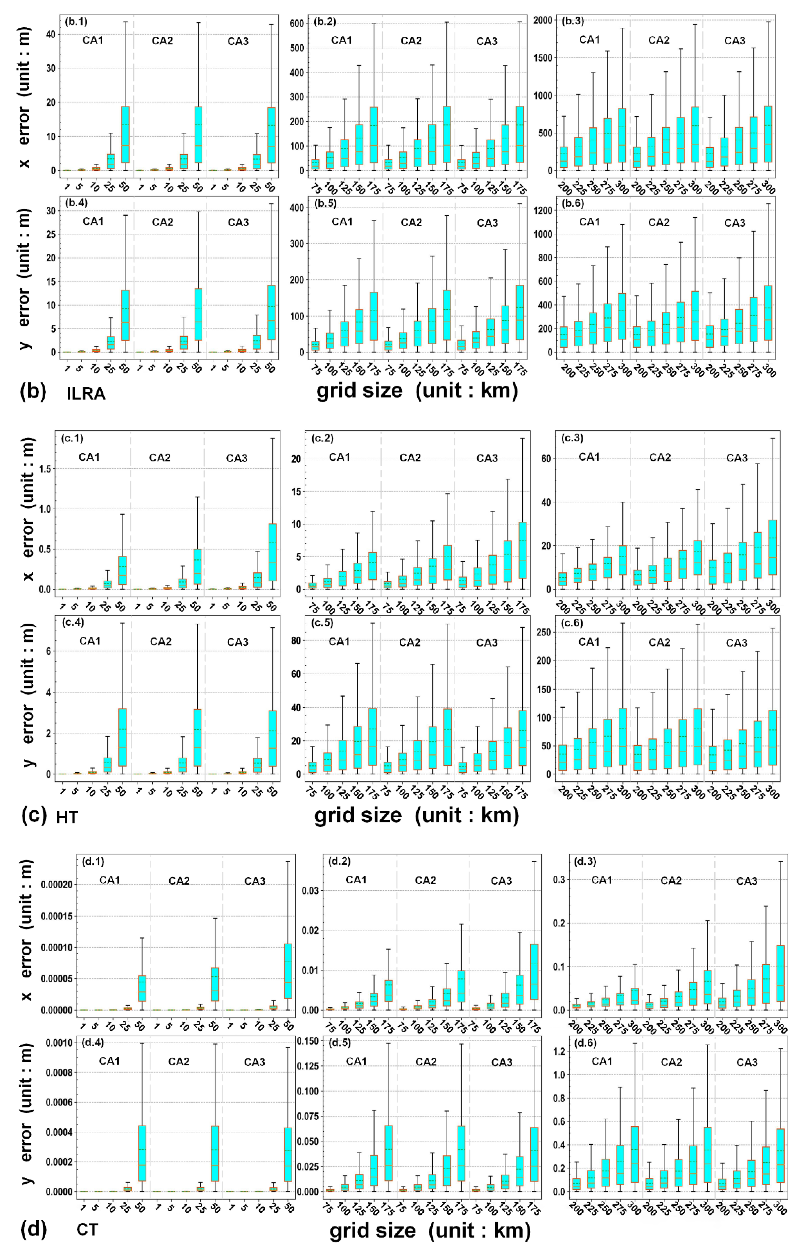
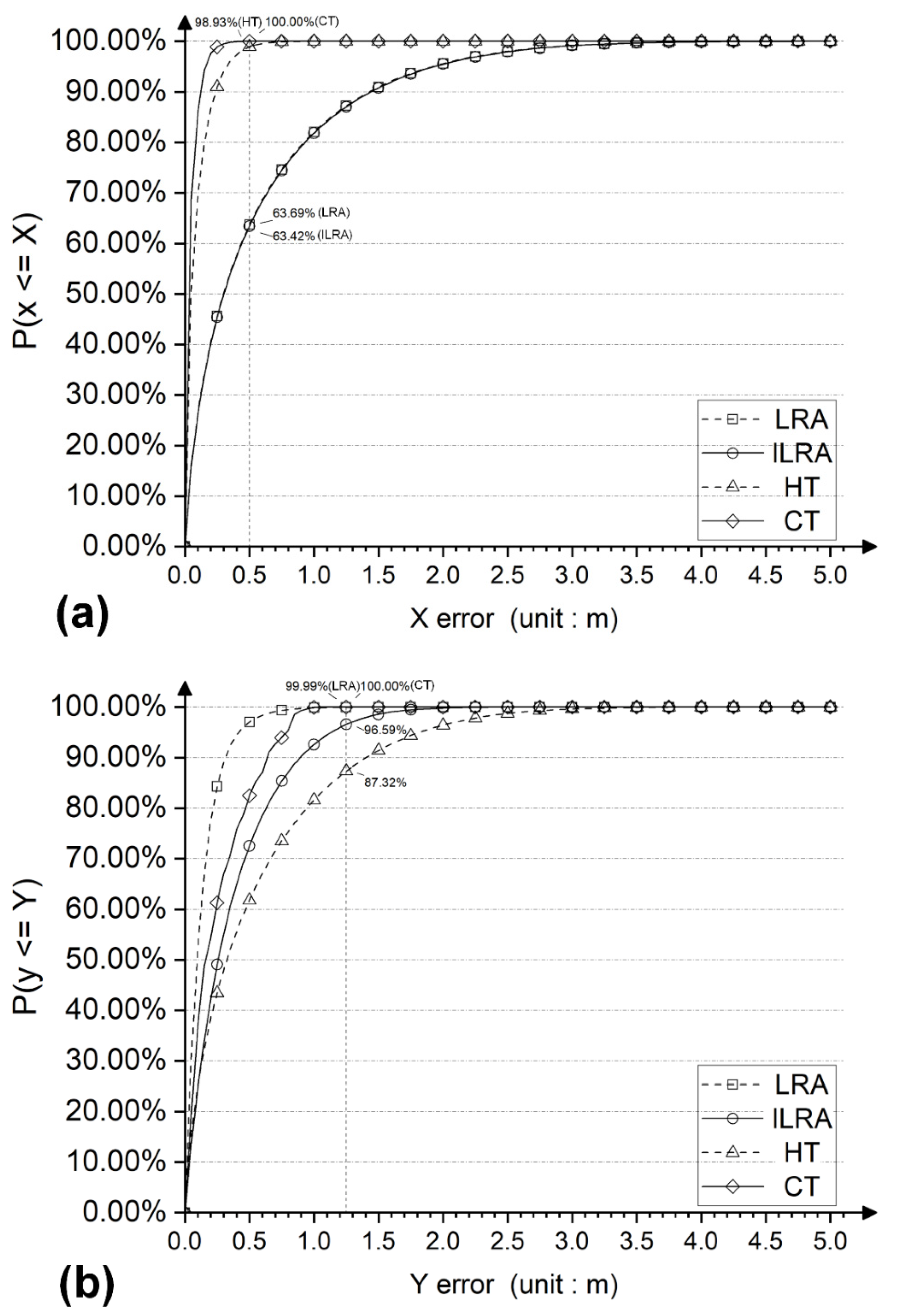
3.1. Error Statistics of Multiple Numerical Methods

The maximum, minimum, mean, and median errors of the linear rule approximation (LRA) method, improved linear rule approximation (ILRA) method, hyperbolic transformation (HT) method, and conformal transformation (CT) method for multiple grid sizes and multiple conversion areas were calculated and expressed as box plots, as shown in Figure 3. First, the x-error and y-error of the CT method are significantly lower than those of the other three methods for the same grid size. However, this does not mean that the other methods are not applicable because the errors can be controlled within the threshold value by controlling the grid size when they are used. Second, the x-error and y-error increase as the grid size increases, and the magnitude of the error increase gradually increases. The CT method has the smallest error increase, the maximum x-error is less than 0.36 m and the maximum y-error is less than 1.22 m when the grid size reaches 300 km × 300 km. The variation characteristics of the x-error of the LRA method and the ILRA method are almost the same, but the y-error of the LRA method is significantly higher than that of the ILRA method. The error is significantly smaller and more stable than that of the ILRA method. For the LRA and ILRA methods, the x-error is larger than the y-error; for the HT and CT methods, the x-error is smaller than the y-error. Third, as the distance between the conversion area and the central meridian of the Lambert projection increases, the maximum value and the dispersion of x- and y-errors of the four methods increase or decrease to different degrees. Among them, the effect of the conversion area change on the HT and CT methods is mainly focused on the x-error, while for the LRA and ILRA methods, the y-error is more affected.

To constrain the maximum error of coordinate transformation to be less than 5 m, we set the grid size of the LRA method, ILRA method, HT method, and CT method to 10 km × 10 km, 10 km × 10 km, 25 km × 25 km, and 275 km × 275 km, respectively. The cumulative error frequency of 33,000,000 sample points in CA2 was calculated, as shown in Figure 4. In terms of x-errors, the CT method has the fastest convergence rate, and the x-error of all sample points is less than or equal to 0.5 m. The percentages of sample points with x-errors less than 0.5 m for the HT method, LRA method, and ILRA method are 98.93%, 63.69%, and 63.42%, respectively. In terms of y-errors, the CT method and the LRA method converged to 1.25 m almost simultaneously. A total of 96.59% and 87.32% of the sample points are less than 1.25 m for the ILRA method and the HT method, respectively. The CT method has the highest comprehensive stability, even though its grid area is 121 times larger than that of the HT method and 756.25 times larger than that of the LRA and ILRA methods.

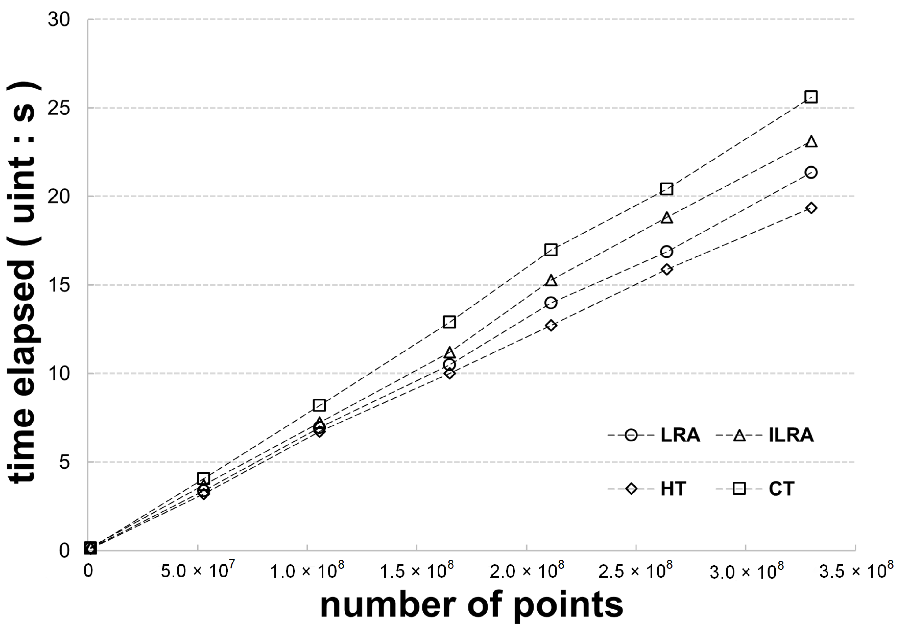
3.2. Comparison of the Transformation Efficiency of Multiple Numerical Methods

The time elapsed of coordinate transformation for the four numerical methods at grid sizes of 10 km × 10 km, 10 km × 10 km, 25 km × 25 km, and 275 km × 275 km was calculated, as shown in Figure 5. The number of sample points is 1.32 × 10⁶, 5.28 × 10⁷, 1.056 × 10⁸, 1.65 × 10⁸, 2.112 × 10⁸, 2.64 × 10⁸, and 3.3 × 10⁸. The coordinate transformation was implemented by a single thread, and the time elapsed was taken as the average of the calculated results for different conversion areas (i.e., CA1; CA2; CA3). The computational time elapsed of the four methods increases linearly with the increase of the number of sample points and is steadily expressed as HT < LRA < ILRA < CT. The time elapsed of the CT method is longer than that of the other methods but with a small difference. The number of grid points of a Sentinel 2 multispectral remote sensing image (spatial resolution: 10 m) is nearly 100 million, and the difference in computation time elapsed is less than 1.5 s when the four numerical methods are executed on a single thread.

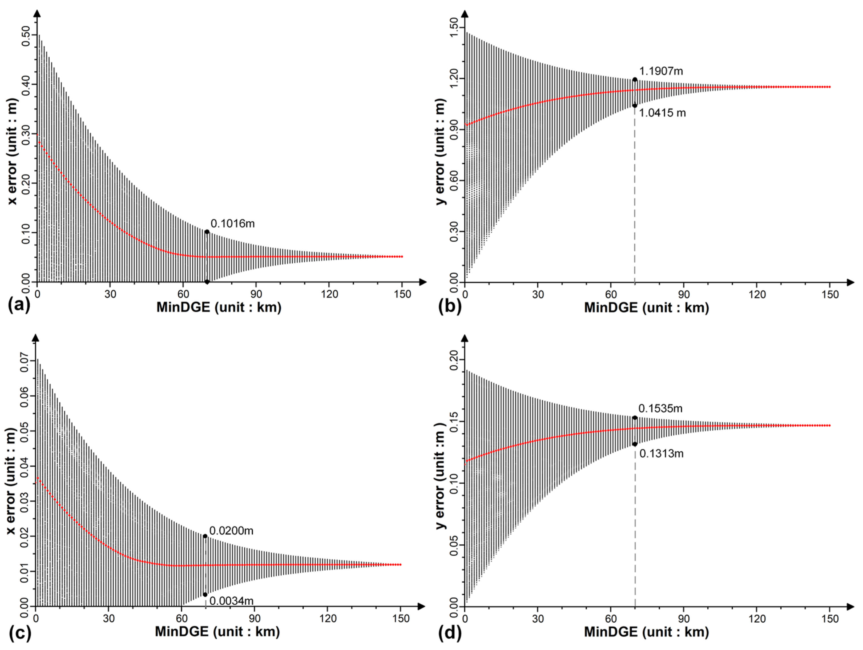
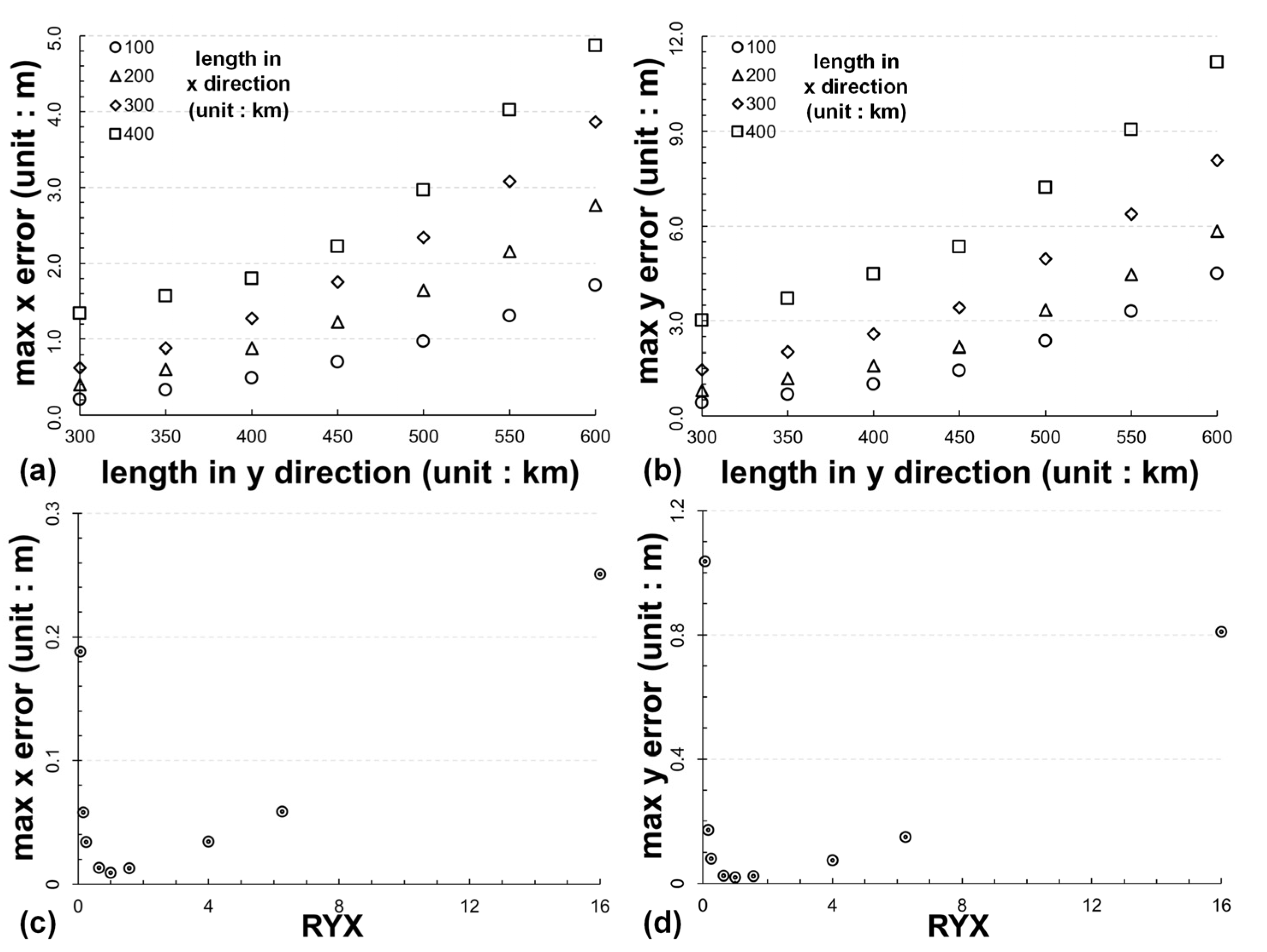
3.3. Effect of Grid Shape Change on the Maximum Coordinate Transformation Error of the CT Method

We used CA1 to calculate the x maximum error and y maximum error of the CT method under different grid shapes and areas. The grid shape and area were adjusted by setting its length in the x-direction to 100 km, 200 km, 300 km, and 400 km, and its length in the y-direction to 300 km, 350 km, 400 km, 450 km, 500 km, and 600 km, as shown in Figure 6a,b.

First, the maximum x-error and maximum y-error both increase with increasing length in the x-direction of the grid, and the increase becomes more drastic when the length in the y-direction of the grid is greater than 450 km. Second, the x maximum error and y maximum error increase with increasing length in the x-direction of the grid when the length in the y-direction of the grid is the same. This phenomenon is mainly caused by the change in the grid area. Third, for the CT method, the grid area is not the only dominant factor affecting the error; another is the grid shape. Setting the grid aspect ratio close to 1 helps to weaken the effect of increasing grid area on the error. For example, in Figure 6a,b, the maximum x-error and maximum y-error of the 300 × 300 (unit: km²) grid are smaller than those of the 200 × 400 (unit: km²) grid and the 100 × w (w = 450, 500, 550, 600) (unit: km²) grid, although the former has a larger grid area than the latter. Similarly, the maximum x-error and maximum y-error of the 400 × 400 (unit: km²) grid are almost the same as those of the 100 × 600 (unit: km²) grid, although the area of the former grid is nearly 2.7 times larger than that of the latter. Fourth, setting the grid size to 300 × 300 (unit: km²) is more suitable for applying the CT method to perform the transformation of the sample point set from the UTM planar coordinate system to the Lambert planar coordinate system because it considers both the grid size and the errors.

In another experiment, the coordinate transformation error of the CT method was calculated by setting the ratio of the length in the y-direction to the length in the x-direction of the grid (RYX) to 16, 6.25, 4, 1.5625, 1, 0.64, 0.25, 0.16, and 0.0625, while keeping the grid area equal to 10,000 km², as shown in Figure 6c,d. The maximum x-error and maximum y-error are minimized when RYX is 1. The error increases as the ratio deviates from 1. In addition, keeping the grid area constant and stretching the grid along the x-direction and the y-direction in equal proportions, the variation of errors is not consistent. The grid with a ratio equal to 1/16 can be regarded as the grid with a ratio equal to 16 placed horizontally, and their stretching ratios are equal, but the maximum x-error of the former is smaller than that of the latter, and the maximum y-error of the former is larger than that of the latter.

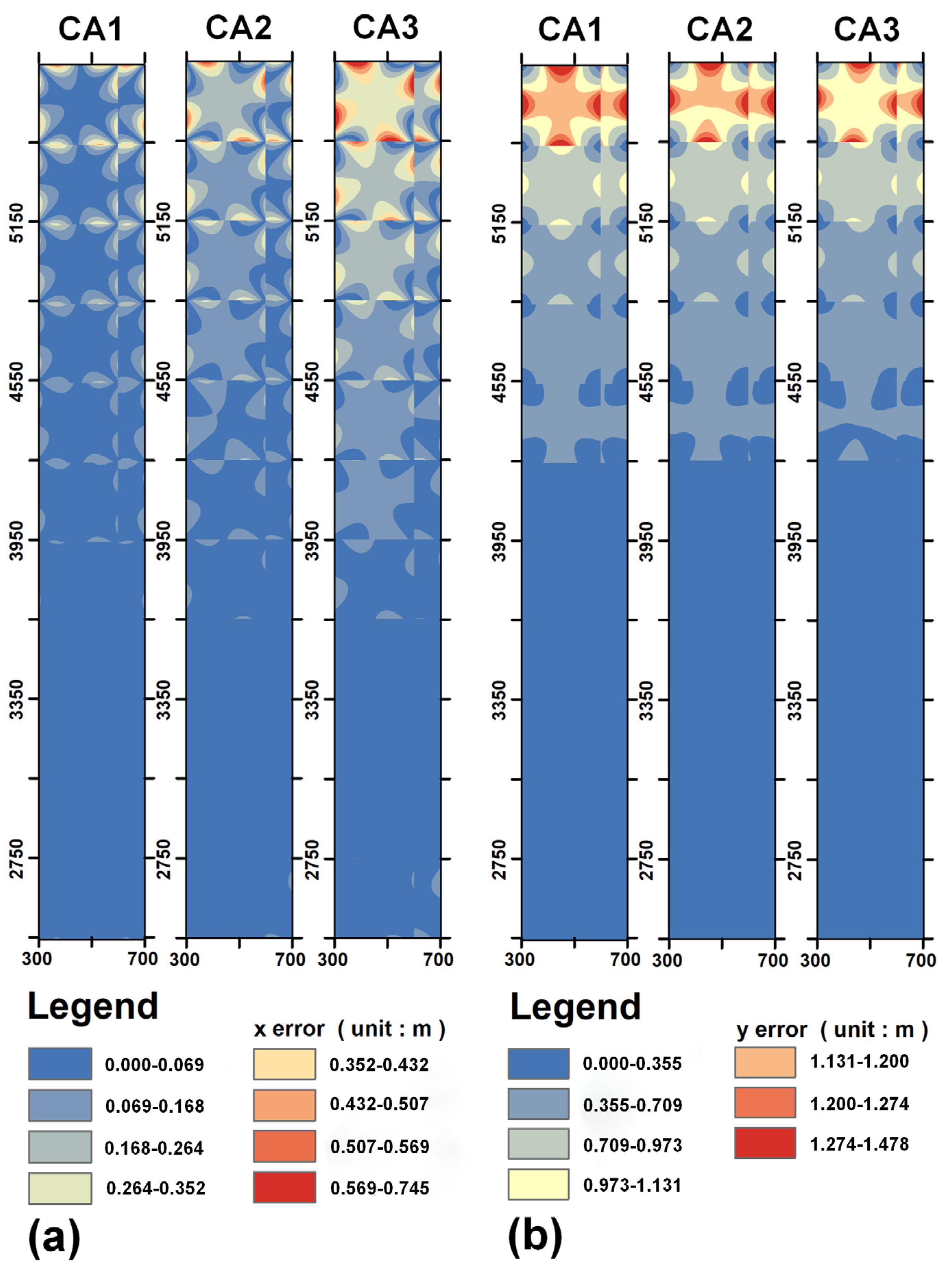
3.4. Spatial Distribution of Coordinate Transformation Error of the CT Method

The spatial distribution of the x-error and y-error of the sample point set was expressed by the raster data model. For each conversion area (i.e., CA1, CA2, and CA3), 33,000,000 sample points were arranged in a matrix of 2000 × 16,500 with a 200 m interval. The applied numerical method was the CT method, and the grid size was 300 × 300 (unit: km²). Considering that the x-error and y-error of the sample point follow the heavy-tailed distribution feature, the head/tail breaks model [22] was applied to the classification rendering of the sample point error.

As shown in Figure 7, first, the x-error and y-error of the sample points all exhibit an overall increasing trend with increasing y-coordinates. For the three transformation regions, the sample points with the largest errors are all distributed in the region with y-coordinates > 5450 km. Second, the x-errors of the sample point exhibit an overall increasing trend as the distance from the sample point to the central meridian of the Lambert projection increases. However, the effect of the distance from the sample point to the central meridian of the Lambert projection on the y-error of the sample point is reversed and concentrated at high latitudes. In the region with y-coordinates > 5450 km, the y-error of some sample points decreases with their deviation from the central meridian. Third, the coordinate transformation error of sample points is also influenced by their positions inside the grid. For each grid, the sample points with the largest and smallest x-error levels are both distributed in a “bow” shape at the edges of the grid. The sample points with the smallest y-error level are concentrated near the four vertices of the grid, and the sample points with the largest y-error level are concentrated in a “bow” shape in the middle of the four edges of the grid. In addition, the distribution of errors within the grid shows symmetric characteristics, with the x-error of the sample point being centrosymmetric and the y-error being axisymmetric.

To further investigate the error distribution within the grid, the two groups of 90,000 sample points were arranged in a 300 × 300 matrix within the specific grid of 300 km × 300 km in CA1. The sample spacing is 1 km, and the coordinates of the vertices of the first grid are (300, 5450), (600, 5450), (600, 5750), and (300, 5750) (unit: km); the coordinates of the vertices of the second grid are (300, 2450), (600, 2450), (600, 2750), and (300, 2750) (unit: km). The x-coordinate intervals of these two grids are the same, but they are 3300 km apart in the y-axis direction. For each sample point in the first grid, the relationship between the coordinate transformation error and its minimum distance to the grid edge (MinDGE, which can be interpreted as the minimum value of the distance from the sample point to the four edges of the grid) is expressed in Figure 8a,b. The dispersion of the error distribution and the maximum error both decrease with increasing MinDGE and stabilize at MinDGE equal to 70 km. The maximum x-error is 25% of the global x-error, and the maximum y-error is 80% of the global maximum y-error for the sample point with MinDGE equal to 70 km. As MinDGE increases, the minimum x- and y-errors of sample points increase, the mean x-error decreases, and the mean y-error increases. As shown in Figure 8c,d, the coordinate transformation error of the sample point near the grid center converges stably and does not change with the y-coordinate of the conversion area. In the two grids, the transformation errors of the sample point stabilize at MinDGE equal to 70 km.

4. Discussion

4.1. Comparison of Multiple Numerical Methods

In this study, the error and efficiency of four numerical methods (i.e., the linear rule approximation method, improved linear rule approximation method, hyperbolic transformation method, and conformal transformation method) were compared in transforming sample point coordinates from the UTM coordinate system to the Lambert coordinate system. The CT method and HT method have their own advantages in applications. The CT method is more suitable for applications with discrete sample point distributions and higher requirements for coordinate transformation accuracy. The HT method can meet the requirements for applications with a relatively concentrated sample point distribution and high requirements for coordinate transformation efficiency. The LRA method and ILRA method have shown poor suitability in our experiments because they are worse than the HT method in terms of coordinate transformation speed and worse than the CT method in terms of transformation accuracy and error convergence speed. The ILRA method is designed to weaken the transformation error of LRA by increasing the number of items in the Taylor series. In this study, however, the error and time elapsed of the ILRA method are higher than those of the LRA method.

The coordinate transformation error of the CT method is influenced by both the x- and y-coordinates of the sample points. The effect of the y-coordinate can be weakened by reducing the grid size as the y-coordinate increases. Another important factor affecting the coordinate transformation error of the CT method is the distance from the sample points to the center of the grid because the sample points with the largest errors are close to the edges of the grid. This error can be reduced by constructing an overlapping grid system. In this strategy, sample points close to the grid edges (i.e., overlapping areas) are inside multiple grids and assigned to suitable grids on their distances to different grid edges.

Table 3. Comparison of coordinate transformation errors between the linear rule approximation (LRA) method, hyperbolic transformation (HT) method, and conformal transformation (CT) method.

Method	Origin Coordinate System	Target Coordinate System	Test Scenario	x/Lon Error	y/Lat Error	Application	Reference
Quartic CT	Mercator projection	Lambert projection	Conversion area: 15 × 15°	≤10.00 m	≤10.00 m	Coordinate transformation for topographic map	[9]
Cubic CT	Mercator projection	Lambert projection	The control points are all on the central meridian, conversion area: 10° × 10°	≤30.00 m	≤30.00 m	Coordinate transformation for topographic map	[9]
HT	Lambert projection	WGS84	Conversion area: 22° × 8°, grid size: 2° × 2°	≤25.25″	≤19.01″	Digitization for paper maps	[12]
HT	Lambert projection	WGS84	Conversion area: 22° × 8°, grid size: 0.5° × 0.5°	≤1.49″	≤1.25″	Digitization for paper maps	[12]
LRA	WGS84	UTM projection	Conversion area: 3° × 3°, grid size: 1′ × 1′	≤0.59 m	≤0.27 m	Large amount of data, high efficiency requirements	[13]
LRA	WGS84	UTM projection	Conversion area: 3° × 3°, grid size: 5′ × 5′	≤6.25 m	≤1.07 m	Large amount of data, high efficiency requirements	[13]

lists the application comparison of the CT method, HT method, and LRA method. All applications met their needs. Yang et al. [9] applied the CT method to the projection transformation of topographic maps, and the transformation in a larger range still maintained low error. Its application value is underestimated, and it can be applied to remote sensing data processing. The HT method and LRA method have been applied to map projections in map digitization and map projections or inverse projections of large amounts of data [12,13].

4.2. Analysis of Potential Application Scenario

The Gauss–Krueger 3 degree/6 degree zonal projection coordinate system is widely used in the organization of regional thematic remote sensing data products in China. The merger and analysis of large-scale thematic raster data require transforming sample point coordinates from the Gauss–Krueger projection coordinate system into the Lambert projection coordinate system. This application requirement can benefit from our results because the Gauss–Krueger projection differs from the UTM projection only in the scale factor.

The Raster Dataset Clean and Reconstitution Multigrid (RDCRMG) was designed for efficient remote sensing data processing and management and has provided support for multiple large data volume studies (i.e., monitoring of vegetation dryness; crop type identification; and arable land quality analysis) [2,23,24,25,26,27,28,29,30]. According to the architecture of RDCRMG, different types of raster images were subdivided into several independent blocks and distributed for storage in different data nodes by using the multigrid as a consistent partition unit. The World Geodetic System 1984 (WGS 84)-based Universal Transverse Mercator (UTM) 6-degree strip division projection coordinate system has been designated as an RDCRMG spatial reference. Partitioned calculation result data should be transformed into the Lambert projection coordinate system for seamless data integration. On that basis, the CT method was most suitable for integration into RDCRMG. In addition, the CT method can be used to improve the coordinate transformation efficiency between the projection coordinate system and global discrete grid system.

5. Conclusions

In this study, four numerical methods (i.e., the LRA method, ILRA method, HT method, and CT method) have been used to convert the raster simulated data from the UTM projection coordinate system into the Lambert projection coordinate system. The transformation error and efficiency of these methods were compared. The relationship between multiple grid layout schemes and the error was explored. The x-error and y-error of the CT method are significantly lower than those of the other three methods at the same grid size. The maximum x-error is less than 0.36 m and the maximum y-error is less than 1.22 m when the grid size reaches 300 km × 300 km. Constraining the maximum error of coordinate transformation to less than 5 m, the CT method has the highest comprehensive stability, even though its grid size is the largest. The computational time elapsed of the four methods increases linearly as the number of sample points increases and can be expressed as HT < LRA < ILRA < CT. The time consumption for coordinate transformations of approximately 100 million points by the four methods are all less than 10 s, showing high efficiency. The difference in time consumption among these methods is less than 1.5 s. Considering efficiency and error, the CT method is more suitable than other methods for the rapid transformation of spatial data from UTM projection into Lambert projection. For the CT method, in addition to the grid area, the grid shape also significantly affects the error. Setting the grid aspect ratio close to 1 helps to weaken the effect of increasing grid area on the error. The x-error and y-error of the sample points both exhibit an overall increasing trend as their y-coordinates increase. The x-error of the sample points shows an overall increasing trend as the distance from the sample point to the central meridian of the Lambert projection increases, while the y-error is the opposite. The coordinate transformation error of the sample points near the grid center converges stably. The dispersion of the error distribution and the maximum error of the sample points both decrease as their minimum distance to the grid edge decreases. Within the 300 km × 300 km grid at different latitude zones, the transformation errors of the sample points stabilize when the minimum distance equals to 70 km. This research can provide a reference for realizing the timely merging, inversion, and analysis of high-frequency remote sensing images.

References

1. Ye, S.; Song, C.; Gao, P.; Liu, C.; Cheng, C. Visualizing Clustering Characteristics of Multidimensional Arable Land Quality Indexes at the County Level in Mainland China. Environ. Plan. A Econ. Space 2022, 54, 222–225. [Google Scholar] [CrossRef]
2. Ye, S.; Ren, S.; Song, C.; Cheng, C.; Shen, S.; Yang, J.; Zhu, D. Spatial Patterns of County-level Arable Land Productive-capacity and Its Coordination with Land-use Intensity in Mainland China. Agric. Ecosyst. Environ. 2022, 326, 107757. [Google Scholar]
3. Fang, L.; Wang, M.; Li, D.; Pan, J. CPU/GPU Near Real-time Preprocessing for ZY-3 Satellite Images: Relative Radiometric Correction, MTF Compensation, and Geocorrection. ISPRS J. Photogramm. Remote Sens. 2014, 87, 229–240. [Google Scholar] [CrossRef]
4. Yu, H.; Cao, N.; Lan, Y.; Xing, M. Multisystem Interferometric Data Fusion Framework: A Three-Step Sensing Approach. IEEE Trans. Geosci. Remote Sens. 2021, 59, 8501–8509. [Google Scholar] [CrossRef]
5. Chen, J.; Xing, M.; Yu, H.; Liang, B.; Peng, J.; Sun, G. Motion Compensation/Autofocus in Airborne Synthetic Aperture Radar: A Review. IEEE Geosci. Remote Sens. Mag. 2021, 2–23. [Google Scholar] [CrossRef]
6. Zhu, Y.; Wang, M.; Cheng, Y.; He, L.; Xue, L. An Improved Jitter Detection Method Based on Parallax Observation of Multispectral Sensors for Gaofen-1 02/03/04 Satellites. Remote Sens. 2019, 11, 16. [Google Scholar] [CrossRef] [Green Version]
7. Ipbuker, C. An Inverse Solution to the Winkel Tripel Projection Using Partial Derivatives. Cartogr. Geogr. Inf. Sci. 2002, 29, 37–42. [Google Scholar] [CrossRef]
8. Wu, Z. How to Transform the Coordinates of One Kind of Map Projection Point to Another Kind of Map Projection Point Coordinate Problem. Acta Geogr. Sin. 1979, 1, 55–68. [Google Scholar]
9. Yang, Q.; Snyder, J.; Tobler, W. Map Projection Transformation: Principles and Applications; CRC Press: Boca Raton, FL, USA, 1999. [Google Scholar]
10. Liu, X.; Liu, H. A Comprehensive Appraisial of Numerical Transformation Method for Map Projection. J. Inst. Surv. Mapp. 2002, 19, 150–153. [Google Scholar]
11. Liu, D.; Zhou, G.; Huang, J.; Zhang, R.; Shu, L.; Zhou, X.; Xin, C. On-board Georeferencing Using FPGA-based Optimized Second-order Polynomial Equation. Remote Sens. 2019, 11, 124. [Google Scholar] [CrossRef] [Green Version]
12. Bildirici, I. Numerical Inverse Transformation for Map Projections. Comput. Geosci. 2003, 29, 1003–1011. [Google Scholar] [CrossRef]
13. Ye, S.; Yan, T.; Yue, Y.; Lin, W.; Li, L.; Yao, X.; Mu, Q.; Li, Y.; Zhu, D. Developing a Reversible Rapid Coordinate Transformation Model for the Cylindrical Projection. Comput. Geosci. 2016, 89, 44–56. [Google Scholar] [CrossRef]
14. Hardy, R.L. Multiquadric Equations of Topography and Other Irregular Surfaces. J. Geophys. Res. 1971, 76, 1905–1915. [Google Scholar] [CrossRef]
15. Hardy, R.L. Theory and Applications of the Multiquadric-biharmonic Method 20 Years of Discovery 1968–1988. Comput. Math. Appl. 1990, 19, 163–208. [Google Scholar] [CrossRef] [Green Version]
16. Zhao, Q.; Duan, M.; Yin, C.; Qin, C. Rapid algorithm of raster map projection transformation. In Proceedings of the Second International Conference on Image and Graphics, Hefei, China, 31 July 2002; pp. 154–159. [Google Scholar]
17. Mu, C.; Chou, T.; Hoang, T.V.; Kung, P.; Fang, Y.; Chen, M.; Yeh, M. Development of Multilayer-Based Map Matching to Enhance Performance in Large Truck Fleet Dispatching. ISPRS Int. J. Geo-Inf. 2021, 10, 79. [Google Scholar] [CrossRef]
18. Yang, Q. On the Numerical Method For transforming The Zones of Gauss Projection. Acta Geod. Cartogr. Sin. 1982, 11, 18–31. [Google Scholar]
19. Yang, Q. A Research on Numerical Transformation between Conformal Projections. Acta Geod. Cartogr. Sin. 1982, 11, 268–282. [Google Scholar]
20. Li, J. A Research on Transformation of Finiteelembnt between Conformal Projections. Acta Geod. Cartogr. Sin. 1985, 14, 214–225. [Google Scholar]
21. Liu, H. The Numerical Method of Transformation of Conformal Projection. Acta Geod. Cartogr. Sin. 1985, 14, 61–72. [Google Scholar]
22. Jiang, B. Head/tail Breaks: A New Classification Scheme for Data with a Heavy-tailed Distribution. Prof. Geogr. 2013, 65, 482–494. [Google Scholar] [CrossRef]
23. Ye, S.; Liu, D.; Yao, X.; Tang, H.; Xiong, Q.; Zhuo, W.; Du, Z.; Huang, J.; Su, W.; Shen, S. RDCRMG: A Raster Dataset Clean & Reconstitution Multi-grid Architecture for Remote Sensing Monitoring of Vegetation Dryness. Remote Sens. 2018, 10, 1376. [Google Scholar]
24. Yang, N.; Liu, D.; Feng, Q.; Xiong, Q.; Zhang, L.; Ren, T.; Zhao, Y.; Zhu, D.; Huang, J. Large-Scale Crop Mapping Based on Machine Learning and Parallel Computation with Grids. Remote Sens. 2019, 11, 1500. [Google Scholar] [CrossRef] [Green Version]
25. Zhang, L.; Liu, Z.; Liu, D.; Xiong, Q.; Yang, N.; Ren, T.; Zhang, C.; Zhang, X.; Li, S. Crop Mapping Based on Historical Samples and New Training Samples Generation in Heilongjiang Province, China. Sustainability 2019, 11, 5052. [Google Scholar] [CrossRef] [Green Version]
26. Yao, X.; Li, G.; Xia, J.; Ben, J.; Cao, Q.; Zhao, L.; Ma, Y.; Zhang, L.; Zhu, D. Enabling the Big Earth Observation Data via Cloud Computing and DGGS: Opportunities and Challenges. Remote Sens. 2020, 12, 62. [Google Scholar] [CrossRef] [Green Version]
27. Ye, S.; Song, C.; Shen, S.; Gao, P.; Cheng, C.; Cheng, F.; Wan, C.; Zhu, D. Spatial Pattern of Arable Land-use Intensity in China. Land Use Policy 2020, 99, 104845. [Google Scholar] [CrossRef]
28. Yan, S.; Yao, X.; Zhu, D.; Liu, D.; Zhang, L.; Yu, G.; Gao, B.; Yang, J.; Yun, W. Large-scale Crop Mapping from Multi-source Optical Satellite Imageries Using Machine Learning with Discrete Grids. Int. J. Appl. Earth Obs. Geoinf. 2021, 103, 102485. [Google Scholar] [CrossRef]
29. Ye, S.; Zhu, D.; Yao, X.; Zhang, N.; Fang, S.; Li, L. Development of a Highly Flexible Mobile GIS-Based System for Collecting Arable Land Quality Data. IEEE J. Sel. Top. Appl. Earth Obs. Remote Sens. 2014, 7, 4432–4441. [Google Scholar] [CrossRef]
30. Wan, C.; Kuzyakov, Y.; Cheng, C.; Ye, S.; Gao, B.; Gao, P.; Ren, S.; Yun, W. A Soil Sampling Design for Arable Land Quality Observation by Using SPCOSA-CLHS Hybrid Approach. Land Degrad. Dev. 2021, 32, 4889–4906. [Google Scholar] [CrossRef]
Figure 1. (a,b) show the distribution of control points based on the UTM projection coordinate system and Lambert projection coordinate system. The corner points A, B, C, and D of the grid and corner points B and D of the adjacent grids are the control points, and G is the sample point whose coordinate is transformed within the grid.
Remotesensing 14 02056 g001
Figure 2. (a) shows the overall distribution of conversion areas. The projection coordinate systems of conversion areas CA1, CA2, and CA3 are UTM Zone 48N, UTM Zone 50N, and UTM Zone 52N, respectively. (b,c) show a series of grid systems for dividing the conversion area. The sizes of the grids are 1 × 1; 5 × 5; 10 × 10; 25 × 25; 50 × 50; 75 × 75; 100 × 100; 125 × 125; 150 × 150; 175 × 175; 200 × 200; 225 × 225; 275 × 275; and 300 × 300 (unit: km2). The yellow and blue areas are some of the areas covered by grids of different sizes.
Remotesensing 14 02056 g002
Figure 3. Box plots (ad) show the x- and y-errors of the linear rule approximation (LRA) method, improved linear rule approximation (ILRA) method, hyperbolic transformation (HT) method, and conformal transformation (CT) method in CA1, CA2, and CA3 with multiple grid sizes. The green dotted line represents the average error, and the orange solid line represents the median error. Where the x error = |x0 − x|, y error = |y0 − y|. x0, y0 are calculated by PROJ, and x, y are calculated by the above numerical method.
Remotesensing 14 02056 g003aRemotesensing 14 02056 g003b
Figure 4. (a,b) show the cumulative percentage of x-errors and y-errors, respectively, for the linear rule approximation (LRA) method, improved linear rule approximation (ILRA) method, hyperbolic transformation (HT) method, and conformal transformation (CT) method.
Remotesensing 14 02056 g004
Figure 5. Time elapsed for coordinate transformation by the linear rule approximation (LRA) method, improved linear rule approximation (ILRA) method, hyperbolic transformation (HT) method, and conformal transformation (CT) method.
Remotesensing 14 02056 g005
Figure 6. (a,b) show the variation of max error of CT method when fixing the length in the x-direction (100, 200, 300, and 400 km) and the length in the y-direction of the grid; (c,d) show the variation of max error of CT method for different RYX with constant grid area (10,000 km2). For a specific grid system, RYX represents the ratio of the grid length in the y-direction to that in the x-direction.
Remotesensing 14 02056 g006
Figure 7. (a,b) show the spatial distribution of the x-error and the y-error of CT method in CA1, CA2, and CA3, with a grid size of 300 km × 300 km. For each conversion area, sample points were organized as 400 km × 3300 km raster data with 200 m as the spatial resolution.
Remotesensing 14 02056 g007
Figure 8. (ad) show the relationship between x-errors or y-errors, and the MinDGE of sample points. The MinDGE represents the minimum distance between the sample point and the grid edge. The number of sample points is 90,000. The coordinate transformation of all sample points was executed by the CT method. The red lines show the average error. The coordinates of the southwest corner point and northeast corner point in (a,b) are (300, 5450) and (600, 5750) and in (c,d) are (300, 2450) and (600, 5750) (unit: km), respectively.
Remotesensing 14 02056 g008