Assessing the Impact of the Loss Function and Encoder Architecture for Fire Aerial Images Segmentation Using Deeplabv3+

Abstract

Wildfire early detection and prevention had become a priority. Detection using Internet of Things (IoT) sensors, however, is expensive in practical situations. The majority of present wildfire detection research focuses on segmentation and detection. The developed machine learning models deploy appropriate image processing techniques to enhance the detection outputs. As a result, the time necessary for data processing is drastically reduced, as the time required rises exponentially with the size of the captured pictures. In a real-time fire emergency, it is critical to notice the fire pixels and warn the firemen as soon as possible to handle the problem more quickly. The present study addresses the challenge mentioned above by implementing an on-site detection system that detects fire pixels in real-time in the given scenario. The proposed approach is accomplished using Deeplabv3+, a deep learning architecture that is an enhanced version of an existing model. However, present work fine-tuned the Deeplabv3 model through various experimental trials that have resulted in improved performance. Two public aerial datasets, the Corsican dataset and FLAME, and one private dataset, Firefront Gestosa, were used for experimental trials in this work with different backbones. To conclude, the selected model trained with ResNet-50 and Dice loss attains a global accuracy of 98.70%, a mean accuracy of 89.54%, a mean IoU 86.38%, a weighted IoU of 97.51%, and a mean BF score of 93.86%.

1. Introduction

Wildfires account for most burnt land in Portugal, which has burnt regions of more than 500 thousand hectares in the past decade. In fact, the number of wild and urban fires has been growing significantly in the recent decades. According to statistical data, in 2021, three thousand hectares of land had been burnt in Portugal due to wildfires. The highest statistics were recorded in 2017, with 520 thousand hectares of green land destroyed by wildfires [1]. As per the nation’s record, Portugal’s total land area was covered by 801 thousand hectares of natural forest, accounting for 24% of the country’s total area, by the year 2010. However, the wildfires drastically reduced the lush green forest environment to 16.8 thousand hectares as per the data recorded by the year 2020 [1]. Peak fire season typically begins in mid-July and lasts around 14 weeks. Between 26 October 2020 and 18 October 2021, 129 genuine fire alerts were registered [2]. These statistics are consistent with those from the previous year [1]. According to October 2020 statistical figure, the region with the most burned area was observed to be the cluster of Guarda, with 304 thousand hectares, accounting for 12% of the total burnt area in Portugal.

The devasting wildfires in Portugal set most of the regions in the country on high alert for fires. Several factors contribute to wildfires [3]; factors like human negligence or other biomes due to lack of awareness toward the environment appear to be some predictable causes of wildfires [4]. Some unpredictable factors include lightning, high atmospheric temperature, or dryness due to global warming with rapid industry growth and air pollution [1]. Moreover, dryness, wind, and humidity in the atmosphere set favorable conditions for the propagation of forest fires [5,6,7]. In turn, it affects the inhabitant of the forest and eco-system to a greater extent. Besides, it impacts the economic growth and harmony of the agricultural and industrial sectors. Thus, generally, it is essential to identify the vulnerable forest fire regions and spot the real fire zones to eliminate unnecessary movement of fire fighters’ teams [8].

The present work addresses the above challenge by implementing an on-site detection framework and spotting the fire pixels in the original picture in real-time. It is achieved by adopting a deep learning architecture, Deeplabv3+ [9], an extended version of the already existing model. This parameter of the Deeplabv3+ is fined tuned with several experimental trails that attain better performance. The experiments were conducted on two public aerial datasets: the Corsican dataset [10] and FLAME [11], and one private dataset, Firefront_Gestosa (The Firefront_Gestosa database is available upon request to the authors.). Compared to the public datasets, the private dataset comprises fewer fire pixels, however not labeled. Thus, for experiments, the data in the private dataset are labeled manually in the present work.

The main contributions of this paper include the following:

-

An in-depth analysis of the impact of different loss function, with different encoder architectures over different types of aerial images is performed. Firefront_Gestosa and FLAME are two dataset of aerial images covering different scenarios. The first set contains very limited fire pixels, less than 1% over the final dataset. The second set contains a higher ratio of fire pixels in comparison to the first one, but it includes some different images of the same view. Usually, the aerial datasets draw segmentation results very low in comparison with the attended performance presented in this paper.

-

Deeplabv3+ parameter fine tuning to train a model in order to efficiently segment aerial images with limited flame area. Moreover, choosing the adequate encoder architecture combined with a proper loss function will reduce the false negatives (FN) and boost the intersection over union (IoU) and BF score.

-

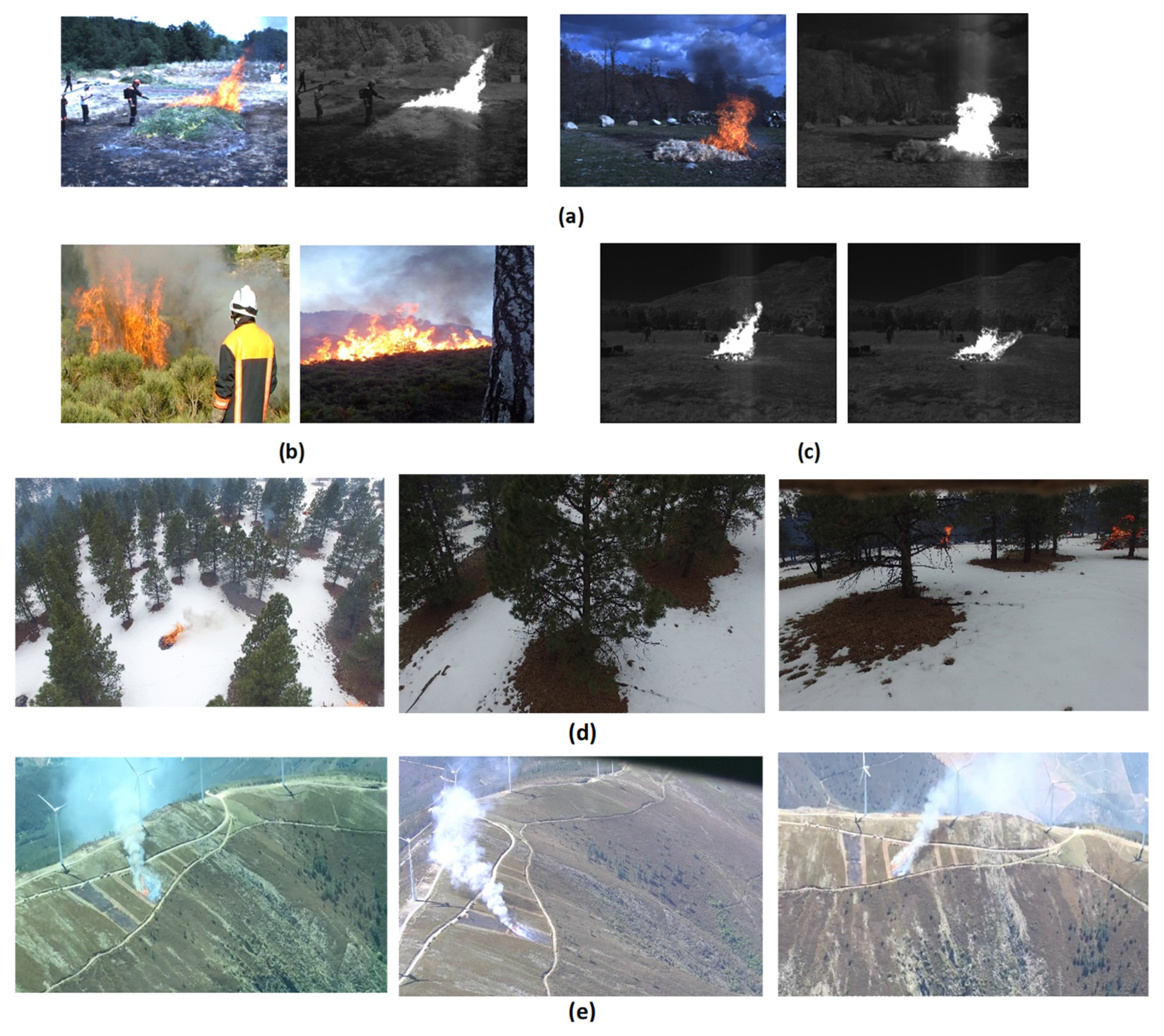
A private labeled set of aerial fire pictures named Firefront_Gestosa dataset has been used in the experiments. The labeling task of such aerial profiles is challenging since the part of smoke sometimes fully cover the flame part. A wrong labeled data while induce a misleading trained classifier. The firefighters are more interested in localizing the exact GPS positions of flames to promptly start intervention to limit the propagation. With huge smoke clouds, it is unbearable to visibly localize the flame positions from soil or air.

The remainder of the paper is organized as follows: Section 2 discusses the related work and the state-of-the-art techniques and its performance in fire pixel detection. Section 3 explains the methods of the proposed framework, detailing the segmentation process of the Deeplabv3+ model with different backbones and loss functions. Moreover, the datasets adopted in the present study are explained with data preparation and processing techniques. Section 4 discusses the experimental setup, and the results of the flame detection are visualized and evaluated in detail. Section 5 summarizes and concludes the present work.

2. Related Work

State-of-the-artwork detects the forest fires utilizing a wide-area sensor network [12,13]; however, the deployment of such a network in a dense forest is expensive and not practical. Alternatively, hyperspectral data may also be utilized in this context for spotting a forest fire in a larger region [14,15,16]. However, it has a low temporal and spatial resolution, thus narrowing down the surveillance area [17,18]. The most often employed method is to acquire visible or infrared images via exploration flights with planes or low-cost drones [19,20]. In most cases, detecting the flame and alarming the firefighters with real fires is a crucial task [21], thus, enabling locating the actual fires and moving the firefighter to the desired location for extinguishing and preventing further fire spread. Several works classify the fire and non-fire region from the image dataset [10,22]. It is broadly categorized into two groups: fire detection (flame detection) [23,24,25] and early fire detection (smoke detection) [26,27,28]. The former detection is challenging, as the smoke persists for hours even after the fire stops, thus making real fire detection more complex, with acquired images or on-site.

State-of-the-art work performs wildfire detection with two strategies: target localization (decision-based techniques) and segmentation [29,30]. Moreover, there are recent studies that had proposed frameworks based on either traditional classification and image processing methods [31,32] or deep learning techniques [33,34]. The latter gained research interest in the past decade for real-time applications that perform faster and more efficient learning on various large image datasets. In recent work, fire segmentation is performed efficiently, adopting a segmentation approach based on traditional methods [29]. Thus, extracting the essential information from near infrared (NIR) and visible images for accurately segmenting the fire images. Furthermore, low and high-frequency components are extracted from visible and IR images of the Corsican dataset [10] using a contourlet-based decomposition. Subsequently, the low-frequency information of visible and IR images is fused utilizing a pulse-coupled neural network (PCNN). While the high-frequency components are fused using the Local log Gabor energy-based fusion rule. Lastly, with implementing the fuzzy C-means clustering (FCM) algorithm, segmentation of images is performed and an accuracy of 98.45% is achieved over the Corsican French dataset [10].

A recent study performed fire segmentation adopting a lightweight deep learning architecture, namely squeezed fire binary segmentation network (SFBSNet) [35]. SFBSNet performed the segmentation adopting the traditional encoder-decoder architecture with depth-wise separable convolution layers that induce a richer feature map. The adopted approach attained a mean Intersection over Union (mIoU) of 90% on a Corsican dataset, highlighting certain model limitations. A recent study implemented Deeplabv3 architecture for fire segmentation on a custom augmented dataset with some image processing algorithms [36]. Experiments were performed on datasets adopting three backbones: ResNet-50, ResNet101, and ResNet-105 and reported a mIoU of 70.51% and an accuracy of 98.78% over the test set.

To summarize, the existing studies on wildfire detection widely focus on segmentation and detection, and adopt suitable image processing techniques in conjunction with machine learning models; thus, drastically reducing the time required for data processing as the time grows exponentially with the size of the acquired images. It is highly essential to spot the fire pixels and alert the firefighters without any delay to handle the situation more responsively in a real-time fire situation. However, most existing systems are modeled for fire segmentation in offline mode, as real-time segmentation and detection necessitate data preprocessing. Thus, it is challenging to perform fire detection and segmentation as it attracts high computational costs.

3. Materials and Methods

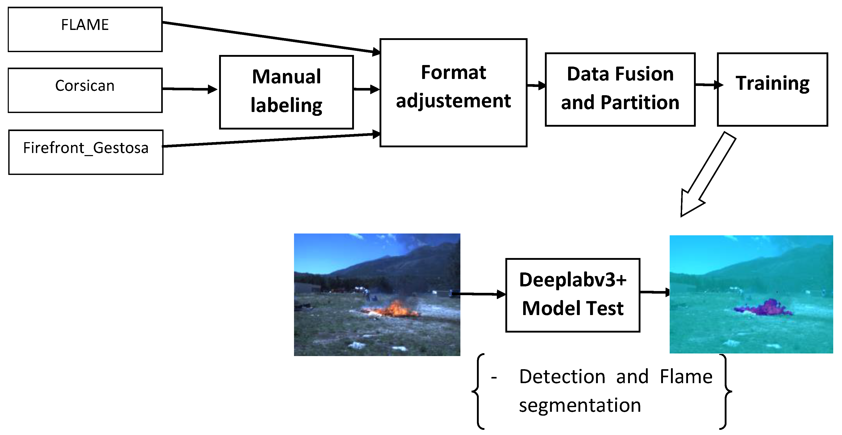
A brief explanation of the segmentation process using deeplabv3+ is explained in this section. Further, the dataset adopted for the present study is described in detail, along with data annotation and augmentation procedure. Figure 1 depicts the framework adopted in the present study for fire segmentation adopting the deeplabv3+ model.

Before implementing the segmentation process, the adopted datasets are labeled manually and annotated accordingly. Subsequently, the labeled or annotated data are partitioned using a data partitioning technique. The adopted datasets were also fused to implement the proposed framework with an increased number of images. It is worth noting that with a few or a limited number of training images, the segmentation process of fire pixels will be challenging. Thus, the model is trained with the images of three different datasets (Corsican [10], FLAME [11], and Firefront_Gestosa [37]) fused for locating the flames in the images. The segmentation mask is generated for fire pixels using the deeplabv3+ model. Performance is measured with global accuracy, mean accuracy, mean IOU, weighted IOU, and mean BF score as assessment metrics.

3.1. Dataset

The present work performed the fire segmentation using the images of public datasets, namely the Corsican dataset [10] and FLAME [11]. Moreover, it performed fire detection with images acquired during the Gestosa mission by the Firefront project team.

3.1.1. Description

The original Corsican dataset [10] comprises almost 2000 wildfires captured with different camera configurations. The pictures were shot in the visible (Please refer to Figure 2b) and near-infrared (Please refer to Figure 2c) spectral ranges at a resolution of 1024 × 768 pixels and stored in portable graphics format (png). The present study selected 1175 pictures from the available image collections, spotting heterogenous color flames with proper background conditions (light and textures). The dataset comprises a collection of multimodal images (see Figure 2a) captured with a “JAI AD-080GE” camera [10]. This sort of camera can simultaneously capture images in the visible and near-infrared spectra using the same optics that are aligned. The Corsican dataset is built adopting a homography matrix transform-based picture registration technique, and every image is annotated with its corresponding segmentation mask.

The FLAME [11] dataset is another public aerial fire dataset adopted in the present study. The FLAME dataset pictures were captured using drones and are primarily composed of videos; some were transformed into frames for segmentation purposes. The designated videos were shot using a Zenmuse X4S and a phantom 3 camera with a resolution of 640 × 512 and a frame rate of 30 frames per second. The dataset consists of 2003 pictures already annotated with corresponding ground truths for every picture.

Firefront Gestosa is an unlabeled aerial private dataset (which will be made public in the future) obtained during the Firefront project team’s Gestosa mission [37]. This dataset primarily consists of five main recorded videos that last between two and three minutes. Please refer to

Table 1. Firefront_Gestosa dataset: The first five videos consist of five main recorded videos. The last video is a compilation of multiple perspectives from the first five videos.

Video	Pixel Resolution	Number of Frames Second (Frame Rate)	Durations in Seconds	Number of Bits per Pixel	Video Format
PIC_081.MP4	1920 × 1080	50	182.88	24	RGB24
PIC_082.MP4	1920 × 1080	50	163.68	24	RGB24
PIC_083.MP4	1920 × 1080	50	178.56	24	RGB24
PIC_085.MP4	1920 × 1080	50	66.24	24	RGB24
PIC_086.MP4	1920 × 1080	50	191.04	24	RGB24
Gestosa2019.MP4	1280 × 270	29.97	218.18	24	RGB24

for further information about each video. The last video is not an actual recording of the mission; it is a compilation of multiple perspectives from the first five videos. Indeed, this dataset poses a significant challenge as it comprises images completely obscured by smoke, making it quite hard to distinguish the flame location from the rest of the image.

Two hundred thirty-eight fire frames were selected for the present study experimentation through the already existing videos. The fire images were manually labeled. More details on the data annotation procedure are explained briefly in the subsequent section.

3.1.2. Data Annotation Technique

The newly extracted images from the Firefront_Gestosa data were labeled manually with pixel labels based on human observation using “MATLAB ImageLabeler”. Following that, the labels were normalized and transformed to binary images.

Table 2. Firefront_Gestosa ground truths preprocessing.

Preprocessing Algorithm
Initialization	For the Mask of Every Picture
Image normalization	Compute minimum and maximum pixel intensity of the mask as follow: $minv=\underset{i=\left\{1, \dots , xsize\right\};j=\left\{1, \dots , ysize\right\}}{\min }\left(mask\left(i,j\right)\right)$ $maxv=\underset{i=\left\{1, \dots , xsize\right\};j=\left\{1, \dots , ysize\right\}}{\max }\left(mask\left(i,j\right)\right)$ xsize and ysize correspond to the number of row and columns of the ground truth picture. The indexed mask is normalized: $nmask=round\left(1+\left(ncol-1\right)\ast \frac{\left(mask-minv\right)}{\left(maxv-minv\right)}\right)$ ncol corresponds to the Number of columns of the used gray map. The function round is used to round the results to the next integer number.
Storing format switch: number colors adjustment	Convert the indexed mask to grayscale image: $rgb\_\mathrm{mask}\left(i,j\right)=\mathrm{nmask}\left(\mathrm{map}\left(\mathrm{i},\mathrm{j}\right)\right)$ map is a matrix defining the gray colormap used. map is an 256 × 3 containing floating-point values of color intensities in the range [0, 1]. Reduce the number of colors and translation to indexed image using Inverse colormap computation algorithm [38], input is rgb_mask and output is ind_mask.
Final step: Switch to binary image	Convert the indexed image to binary format: $\{\begin{array}{c}bn\_mas{k}_{ind\_mask\left(i,j\right)}=1, if ind\_mask\left(i,j\right)\ge \gamma \\ bn\_mas{k}_{ind\_mask\left(i,j\right)}=0, if ind\_mask\left(i,j\right)<\gamma \end{array}$ $\gamma$ is the luminance threshold, the adopted value is 0.5. Save the mask in binary/categorical format.

summarizes the preprocessing steps adopted in the present study. The mask variable refers to ground truth pictures. First, the indexed ground truth images were normalized and then transformed to grayscale pictures.

Furthermore, an inverse colormap algorithm [38] was applied to convert the pictures again to indexed values. The algorithm quantizes the colormap into 2⁵ distinct nuance degrees per color component. Later, the closest nuance in the quantized colormap is localized for each pixel in the grayscale image.

The main objective of the transformations mentioned above (indexed to grayscale and grayscale to indexed) is to have images that deploy a fixed colormap to make the processing easier later. Then the images are binarized based on a threshold value and stored correctly.

The same preprocessing steps were applied to the FLAME dataset that was already labeled. However, before training the models, it was required to convert infrared photos of Corsican data to RGB storage format by simply duplicating the content of the red channel over the green and blue ones.

3.1.3. The Final Dataset

Table 3. Statistics about the data used to train and test the detection module in terms of the number of samples.

Dataset	Corsican Dataset	FLAME	Firefront_Gestosa	Total
Fire pictures	1775	2003	238	4016

summarizes the contribution of each dataset to the simulation data generated by the present study in terms of fire images. It is to be noted that the simulation data generated with fire images contributes to the present work in terms of new data generated from existing data. However, the final dataset’s pixel distribution before scaling is shown in

Table 4. The pixel distribution of our final dataset and the fire pixel contribution in terms of percentage.

Dataset	Corsican Dataset	FLAME	Firefront_Gestosa
Fire pixels count	2.95 × 108	9.71 × 107	1.77 × 105
Background pixels count	1.72 × 109	1.66 × 1010	6.58 × 108
Contribution in final dataset in terms of percentage (%)	24.74	75.22	<1

. The resulting newly created dataset is extremely unbalanced, with Corsican data having the highest amount of fire pixels (Please refer Table 4) in contrast to the other two aerial datasets. Indeed, aerial datasets include fire captures from extremely high altitudes, providing a very distant view of the flame. As a result, the detecting task becomes more challenging.

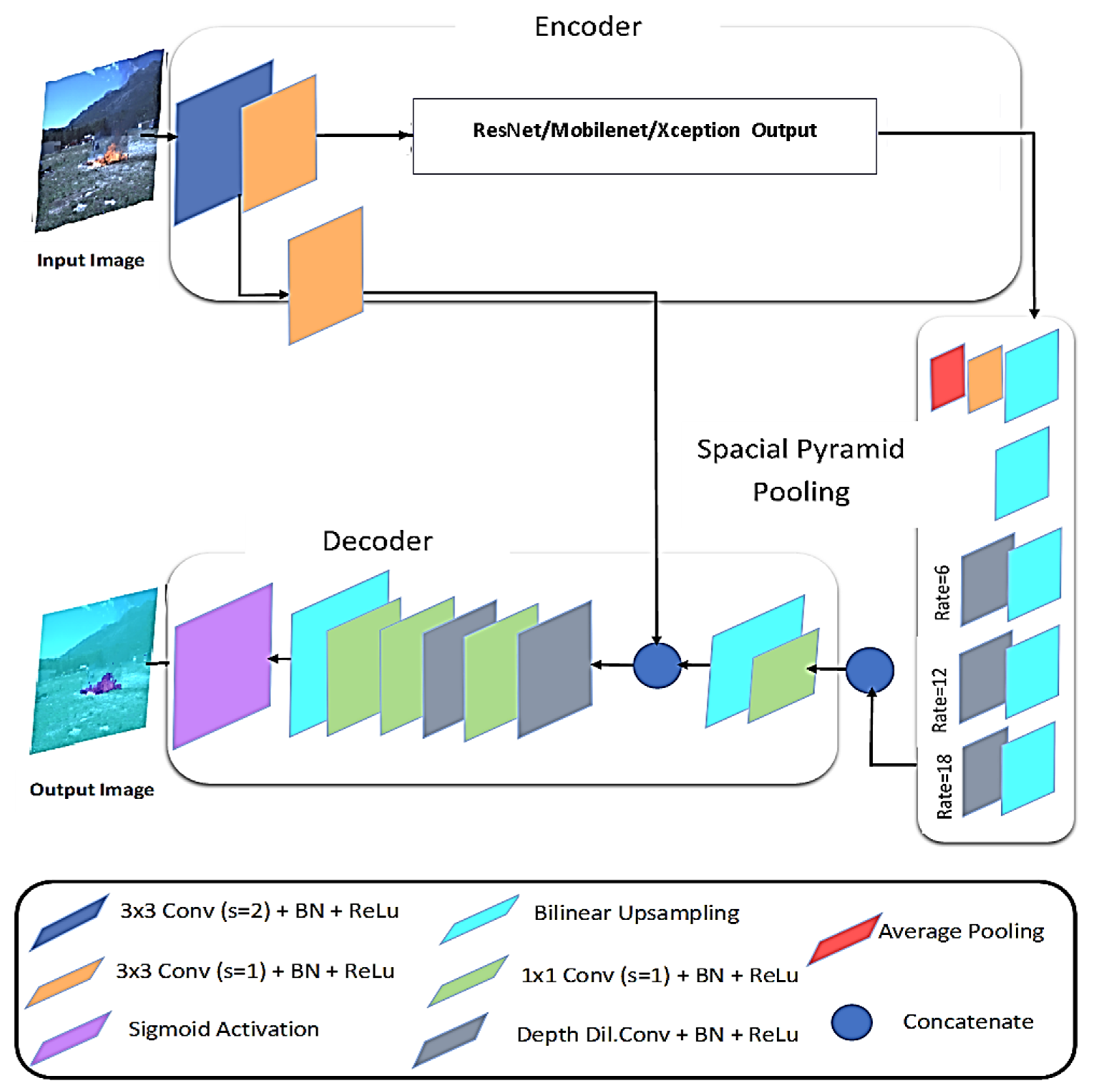
3.2. Segmentation Approach

3.2.1. DeeplabV3+

DeepLabv3+ is an extension of DeepLabv3 architecture that includes an encoder and decoder structure that help the model work more efficiently. Dilated convolution is used by the encoder module to deal with multiscale contextual information, whereas the decoder structure improves the segmentation performance by focusing on object boundaries. Thus, the encoder–decoder architecture is adopted by Deeplabv3+ [9] in the present study. The model is divided into three blocks: encoder, effective decoder, and a spatial pyramid pooling block, as shown in Figure 3. To create a rich feature map, the encoder uses dilated or atrous convolution at different rates [9]. The present work applies an atrous convolution to each location on the output and filter, where the rate of convolution corresponds to how quickly the inputs are sampled. We can maintain a constant stride while increasing the field of view using atrous convolution without increasing the number of parameters or the amount of computation. Finally, a larger feature map is obtained through this process as an output, that enhances the segmentation process.

Later, these features are bilinearly upsampled by a factor of four and combined with the low-level output of the backbone. To ensure information integrity and minimal computational cost, a 1 × 1 convolution is applied to the obtained features to limit the number of channels. The present work utilized multiple backbone types as encoders for experimental simulations, namely ResNet-18 [39], ResNet-50 [40], MobileNetV2 [41], Xception [42], and InceptionResNetV2 [43]. In the final section of the decoder, 3 × 3 convolutions and bilinear upsampling are further applied for obtaining an affine feature map.

3.2.2. Loss Function

The present work conducted multiple experiments employing sophisticated loss functions that address the unbalancing data problem, such as Generalized Dice [44], Tversky [45], and focused [46] loss functions, in addition to the conventional binary cross-entropy [47] loss function.

Let us define x_0i and x_1i as the probability of the i^th pixel to be a fire and non-fire, respectively. Let us also take the ground truth annotated as y_0i/y_1i.

• The Cross-entropy loss: It is the default function with the deeplabv3+ model. It is formulated as follows [47]:

  $$T_{ce}=-\left({\displaystyle \sum }_{i=1}^N{y}_{0i}\log x_{0i}+{\displaystyle \sum }_{i=1}^N{y}_{1i}\log x_{1i}\right)$$

  (1)

  where N corresponds to the number of classes in the dataset.

• Generalized dice loss: The mathematical formulation alleviates the class imbalance problem. The function is given as follows [44]:

$$T_{dc}=1-2\frac{{{\displaystyle \sum }}_{i=1}^N{x}_{0i}{y}_{0i}}{{{\displaystyle \sum }}_{i=1}^N{x}_{0i}+{{\displaystyle \sum }}_{i=1}^N{y}_{0i}}$$

(2)

The function weights the contribution of each class to the final loss by the inverse size of the expected region.

A negligible non-null constant is further introduced in the denominator to avoid invalid values during training.

• Tversky loss: The loss function is defined as follows [45]:

$$T_{tv}\left(a,b\right)=\frac{{{\displaystyle \sum }}_{i=1}^N{x}_{0i}{y}_{0i}}{{{\displaystyle \sum }}_{i=1}^N{x}_{0i}{y}_{0i}+a{{\displaystyle \sum }}_{i=1}^N{x}_{0i}{y}_{1i}+b{{\displaystyle \sum }}_{i=1}^N{x}_{1i}{y}_{0i}}$$

(3)

The parameters a and b allow to adequately tune up the weights of false positives (FPs) and false negatives (FNs). The fact of deploying a value of “b” higher than “a” emphasizes FPs, diminishes the FNs, boosts the recall factor, and favorably improves the training process.

• Focal loss: It is a variant of the original cross-entropy loss that performs class weighting by down-weighting the contribution of every class with a corresponding modulating factor. The following equation gives the mathematical formulation: [46]

$$T_{fc}\left(\alpha ,\gamma \right)=-\left({\displaystyle \sum }_{i=1}^N\alpha {\left(1-y_{0i}\right)}^{\gamma }\log x_{0i}+{\displaystyle \sum }_{i=1}^N\alpha {\left(1-y_{1i}\right)}^{\gamma }\log x_{1i}\right)$$

(4)

The α value scales the loss function linearly while Y is the focusing parameter of the function. Increasing the value of Y improves the sensitivity of the trained network. The optimal value of α is 0.25, and Y is 2 [46].

3.2.3. Assessment Metric

The metrics used to access the performance of the segmentation models are: global accuracy, mean accuracy, mean IoU, weighted IoU, and mean BF score.

• Global accuracy is a more general metric that gives insight into the percentage of correctly classified pixels without considering the classes. This metric is completely misleading in the case of highly unbalanced datasets.
• Mean accuracy gives an idea about the portion of correctly classified pixels considering all the classes. Mathematically defined as:

  $$Accuracy=\frac{TPs}{TPs+FNs}$$

  (5)

  where TPs is the number of true positives, the number of positive pixels correctly classified.

• Mean IoU or Jaccard similarity measure, computed as the average IoU measure of all data classes calculated for all the images and averaged. In other words, it is a statistical measure of precision that penalizes FPs. IoU (or Jaccard) metric is mathematically defined as:

$$IoU=\frac{TPs}{TPs+FPs+FNs}$$

(6)

• Weighted IoU is a measure that considers the minority classes in unbalanced datasets. Hence, the overall score is more realistic. This metric is defined as the mean IoU of each class in the data, weighted by the number of pixels in that class.
• Mean BF Score, the boundary F1 contour matching score, mathematically defined by the following formula:

$$BF=\frac{TPs }{ TPs+0.5\ast \left(FPs+FNs\right)}$$

(7)

The mean BF score is pointed as the mean value of the BF score calculated overall images for a corresponding class. This metric measures the degree of matching of the object contours (prediction) and the given ground truth.

4. Experiments

4.1. Experimental Setup

The segmentation model was experimentally evaluated with 20 different configurations. Deeplabv3+ is used with four distinct loss functions (Cross-Entropy, Dice, Tversky, and Focal loss) and five different backbones: ResNet-18, ResNet-5, MobileNetV2, Xception, and InceptionResNetV2. The models are improved and trained in the MATLAB environment, installed on a server equipped with an NVIDIA GeForce RTX 3090 GPU and the Fedora operating system at the IT-Lisbon facility.

Image of resolution of 512 × 512 pixels is chosen with mini-batch size of 22 to obtain the most significant information at the lowest computing cost. Stochastic gradient descent (SGDM) optimizer with a momentum of 0.9 and a piecewise schedule learning rate method is used for training the model. The learning rate drop period is set to 10 with the dropping factor and initial learning rate assigned as 0.3 and 0.01, respectively. The maximum number of training epochs was set to 100, with the L2 regularization factor as 0.0005. These chosen parameter choices were assumed to have a rapid learning rate while converging to an optimal solution when the learning rate drops. The experiments are parameterized to avoid overfitting by terminating training sooner when the validation curve converges.

Every convolutional layer in the trained network is followed by a Batch Normalization layer, which improves training stability, speeds up network convergence, and improves performance even when the batch size is small. The parameters a and b are set to 0.3 and 0.7 for the Tversky loss function and 0.25 and 2 for the focal loss function, respectively.

The final dataset was randomly divided into 60% for training, 20% for validation, and 20% for testing for five-fold cross-validation. As a result, 2410 samples were used for training, 803 for validation, and 803 for testing.

Besides, the present work performed experiments with data augmentation to increase network accuracy during training by randomly transforming the original data. As augmentation techniques, random horizontal/vertical reflection, random left/right reflection, random X/Y translation of ± ten pixels, and random rotation were employed. The results were the same as the original, with no remarkable enhancement for augmented data, so the present work refers only to show the original results.

4.2. Implementation and Results

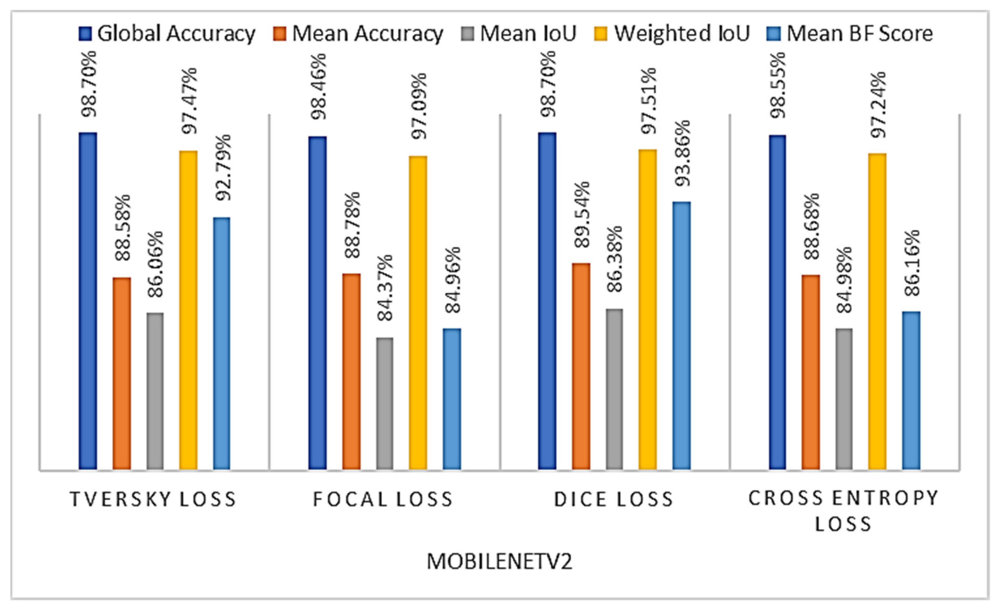
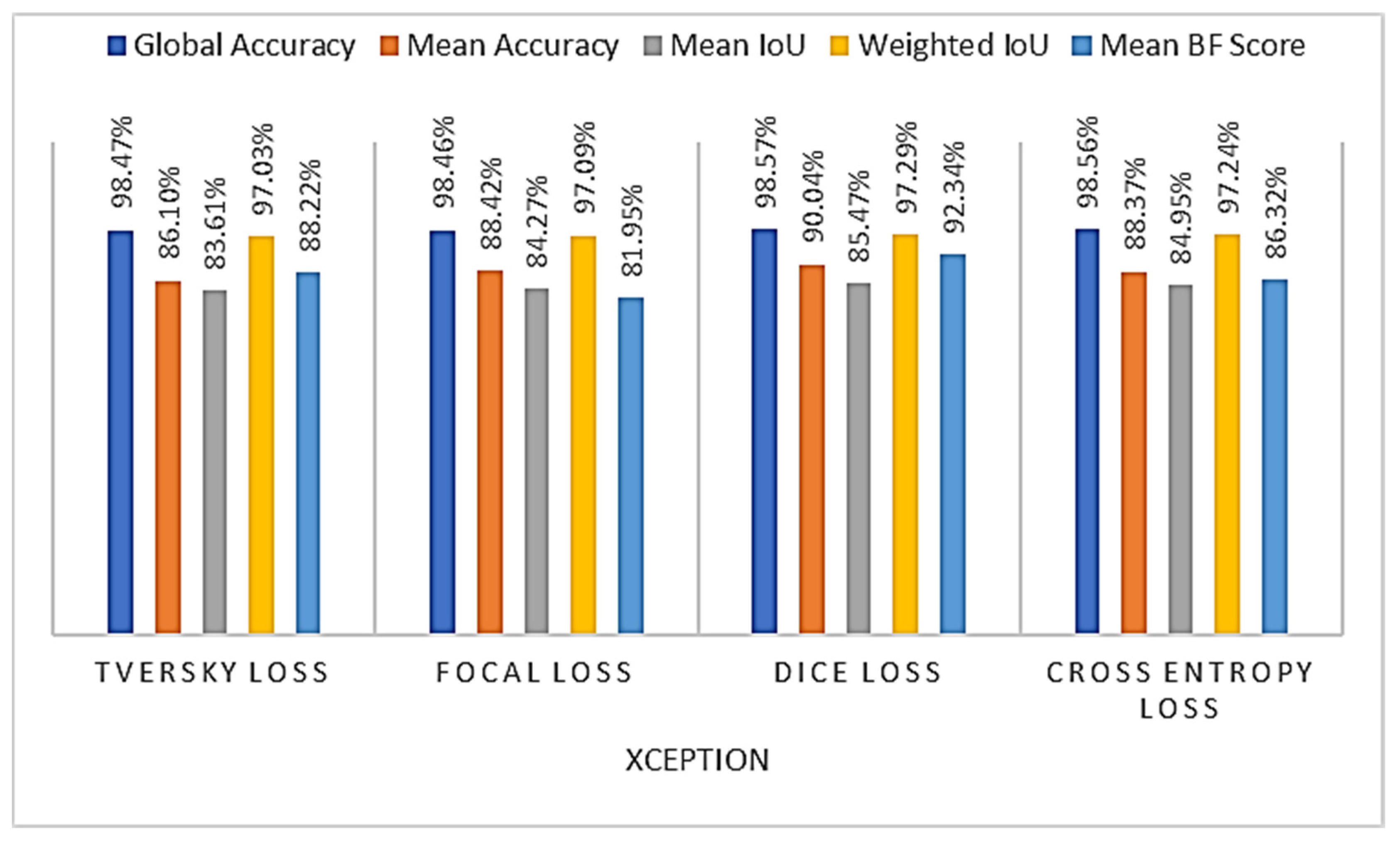
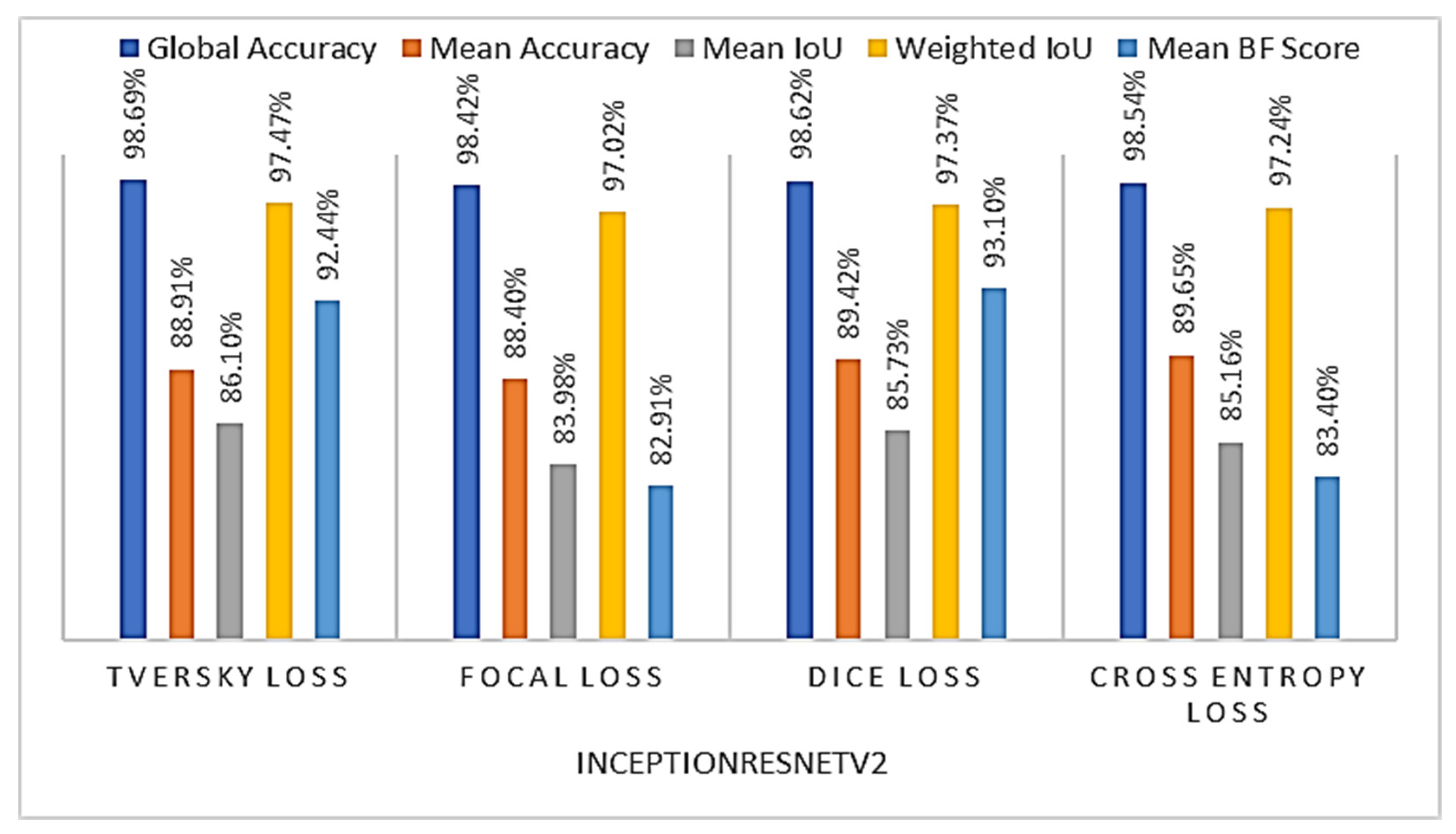
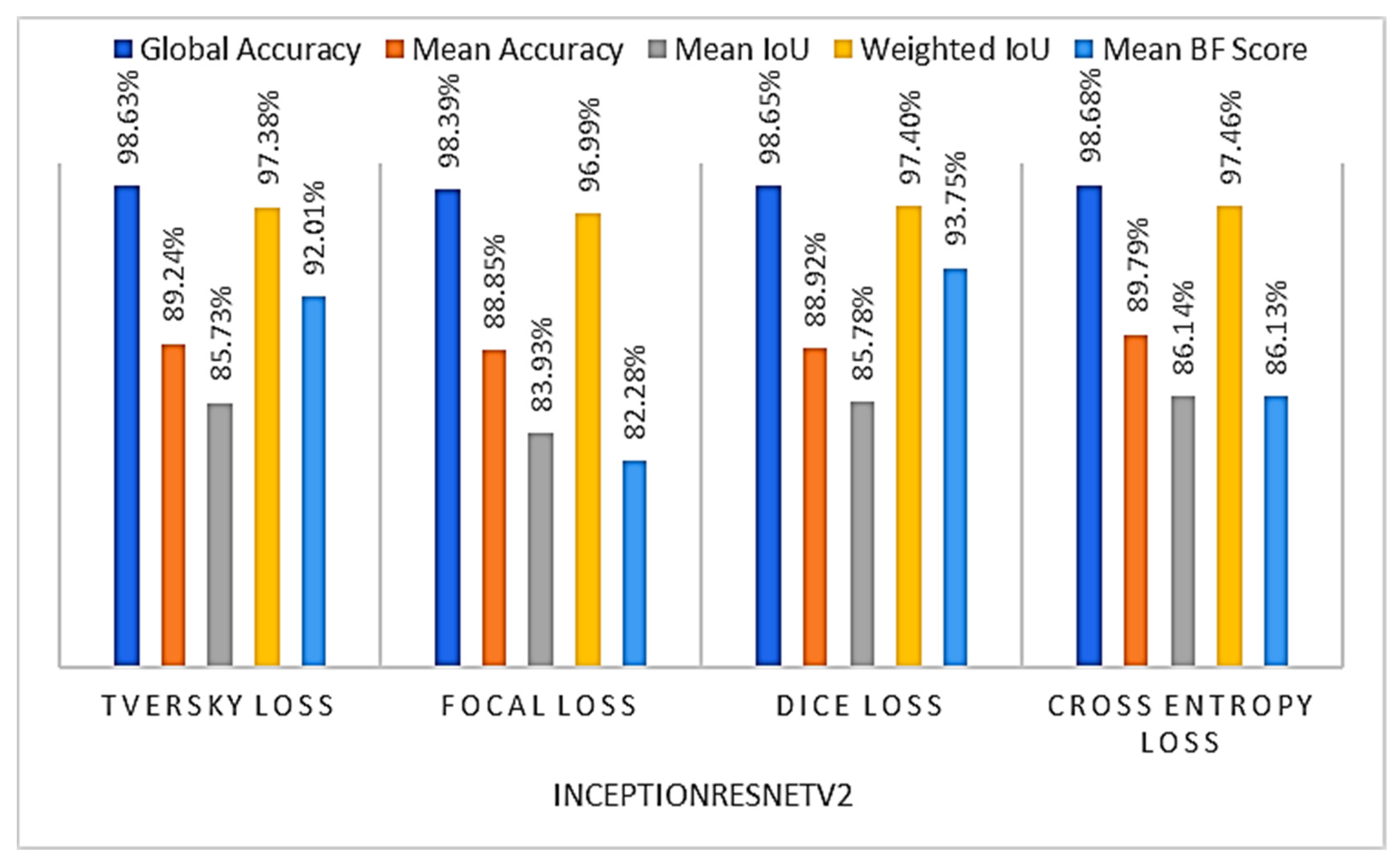
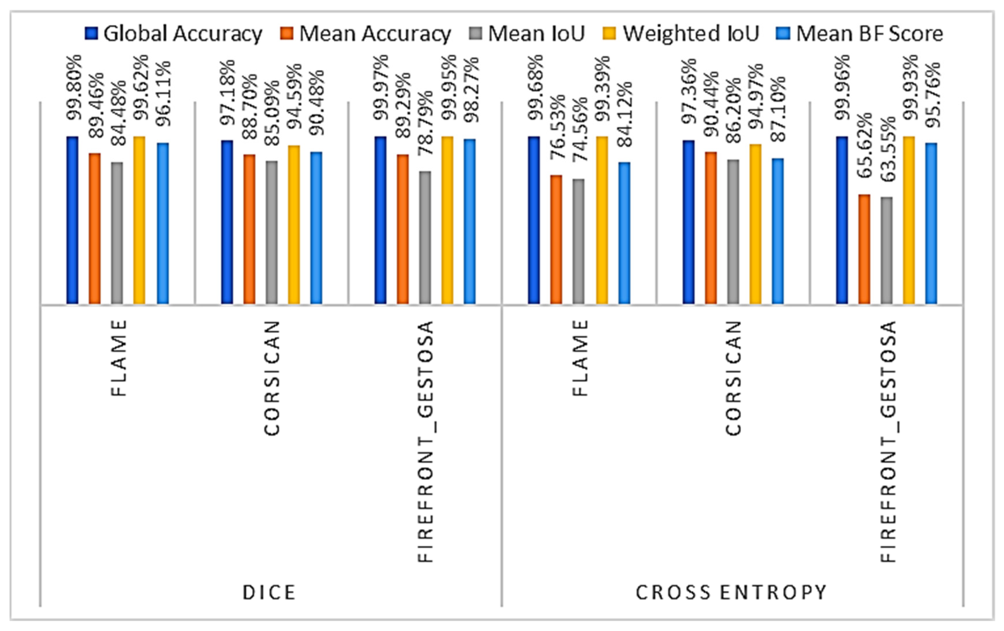
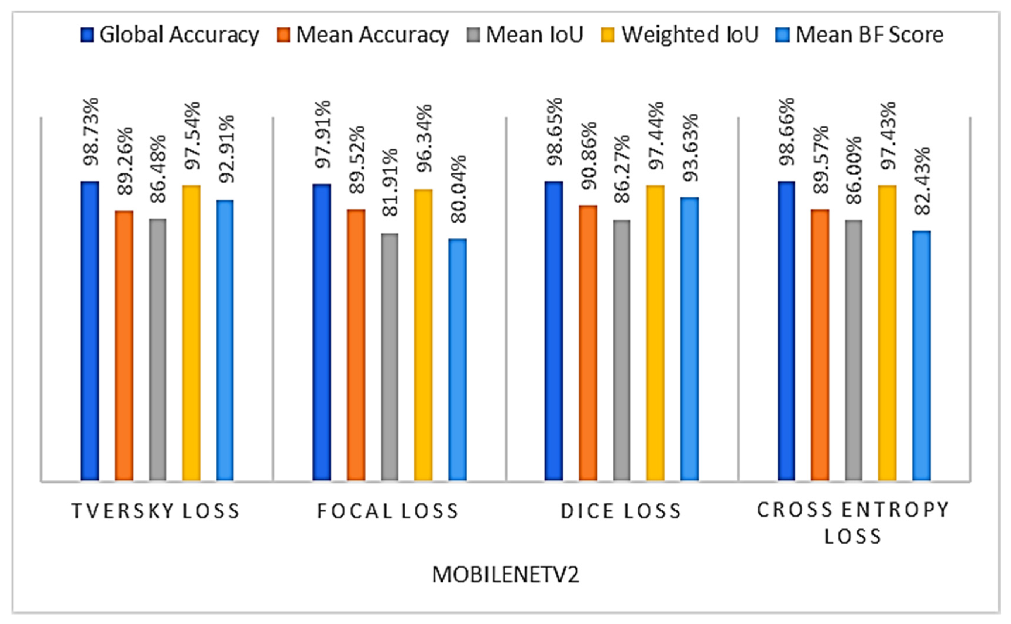
4.2.1. Loss Function Choice

The overall results for deeplabv3+ using MobileNetV2 and Xception within the four different loss functions previously introduced are given in Figure 4 and Figure 5 respectively. All the scores are expressed in percentage (%).

For the case of MobileNetV2, the model trained with the Dice loss function draws the higher results, a global accuracy of 98.70%, a mean accuracy of 89.54%, a mean and a weighted IoU of 86.38% and 97.51%, respectively, and a mean BF score of 93.86%. This model is named Model_1.

In fact, in the model’s selection process, the present study focused on the IoU metric more than the BF score even though the first one gives a better idea about the mask correspondence with the ground truth.

The IoU and BF scores seem equivalent for a single instance classification; however, averaging the results over an entire dataset is completely different. The IoU gives better insights into the number of misclassified instances, while the BF score gives the pixel-level squaring error. Hence, the BF score averages while the IoU metric characterizes the worst situation performance.

The global and the mean accuracy metrics do not correspond with our expectations of the real segmentation performance for highly imbalanced datasets. Since the BF score mathematical formulation does not consider the number of true negatives (TNs), a large value of TNs will not affect the BF metric. However, for the models trained with Xception, the highest results are recorded also using the Dice loss function. The selected model, named Model_2, achieves a global accuracy of 98.57%, a mean accuracy of 90.04%, a mean, and a weighted IoU of 85.47% and 97.29%, respectively, and a mean BF score of 92.34%.

The overall results for deeplabv3+ trained with InceptionRestNetV2 within the four different loss functions previously introduced are depicted in Figure 6. The models trained with Tversky and Dice loss functions draw high and approximatively similar mean IoU values. As a result, determining the best model based on these values was challenging. Hence, to describe the behavior of the two models, a deeper investigation of the performance across all datasets was necessary at this stage.

The two models testing results over the three sets of data, FLAME, Corsican, and Firefront_Gestosa, are depicted in Figure 7. The chart depicts that the model trained with Dice loss performs better over the two aerial datasets, FLAME and Firefront_Gestosa. Over Corsican data, the model trained with Dice loss performs as well as the one trained with Tversky loss. The main goal of the present work is to create a model that can properly segment fire images captured from aerial datasets with extremely small flame regions. Hence, the present study focused on the performance over the biggest aerial dataset, FLAME, followed by Firefront_Gestosa, with limited flame areas. The model trained with Dice loss and InceptionResNetV2 is named Model_3.

However, the results for deeplabv3+ trained with RestNet-18 within the four different loss functions previously introduced are depicted in Figure 8. The models trained using the Dice and Cross entropy loss functions produce nearly identical results. Hence, it was crucial to analyze the results individually over every set of data.

The chart of Figure 9 presents the results of the models trained with Dice and Cross entropy loss functions over every data set. We could conclude that the model trained with Dice loss performs substantially better than the others over the two aerial datasets in terms of mean accuracy, mean IoU, and BF score. The model trained with Cross entropy shows bit higher results over Corsican data, which is the set of data with the higher quota of Fire pixels in terms of mean accuracy and mean IoU. So, the overall results tend to elite this model as the best one. Nevertheless, the model trained with Dice loss draws the best results over the most challenging aerial datasets. This model, named Model_4, achieves a global accuracy of 98.65%, a mean accuracy of 88.92%, a mean, and a weighted IoU of 85.78% and 97.40%, respectively, a mean BF score of 93.75%.

Nonetheless, the results for deeplabv3+ trained with RestNet-50 within the four different loss functions previously introduced are depicted in Figure 10. Both models trained within the Dice and Tversky loss functions show similar results in mean IoU even though the one trained with Dice overpassed the one trained with Tversky in terms of mean accuracy and BF score. So, it was necessary to analyze the results over every set of data individually.

The chart of Figure 11 present the results of the models trained with Tversky and Cross entropy loss functions over every data set. The model trained with Tversky loss gives a higher value of mean IoU and mean BF score over the Corsican set. Although the model trained with Dice loss attains the best results in terms of mean accuracy, mean IoU, and mean BF score over the two aerial sets of data. This model, named Model_5, reaches a global accuracy of 98.65%, a mean accuracy of 90.86%, a mean and a weighted IoU of 86.27% and 97.44%, respectively, and a mean BF score of 93.63%.

To resume, cross-entropy loss in her original formulation could not handle imbalanced data problems and complex data cases.

The dice loss concentrates on the positive sample regions and is less sensitive to the imbalanced data problem. Tversky loss relies on the principle of weighing FN and FP by tuning the value of b bigger than a to penalize FN. However, this function remains a tentative improvement of the Dice function to have more control over loss in case of unbalanced datasets to promote the results of the segmentation of small-scale objects.

Nonetheless, focal loss introduces a mathematical constant ($1-\gamma$) that causes less sensitivity to the imbalanced data problem. Furthermore, this function is better suited to locate small and fine boundary objects that are difficult to identify accurately, and it can handle complicated misclassified data samples.

Those two improvements of Dice loss allow detecting small-scale objects with finer boundary, which is evident through the results, i.e., a slight improvement of the metrics over Corsican data in most cases. This set has the bigger contribution of pixel fires in the final dataset. However, as previously stated, the proposed framework is more suited for aerial data, making it more challenging owing to the lack of publicly available data for training.

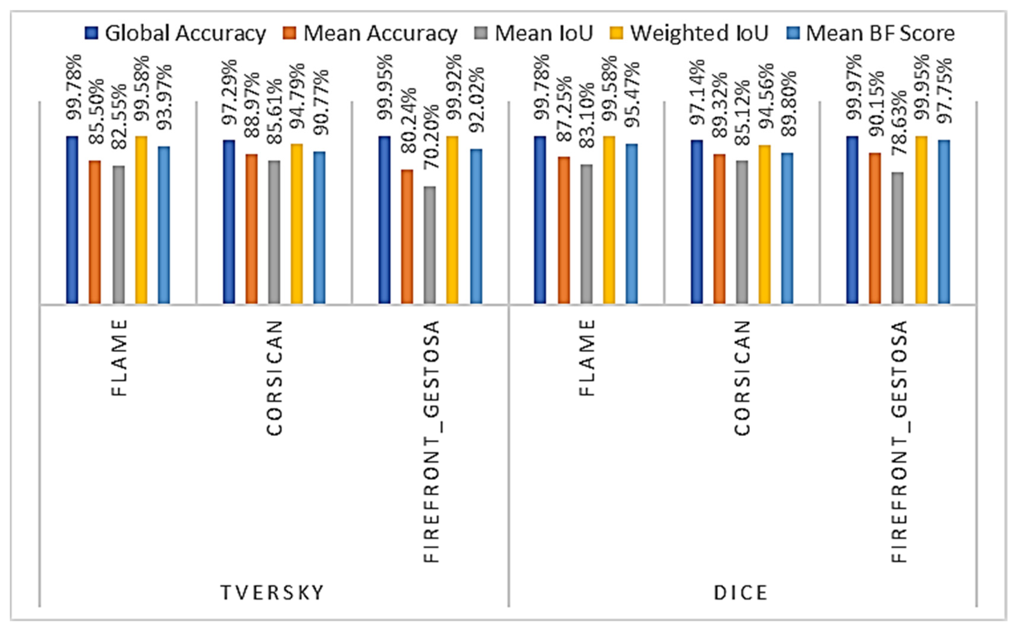
4.2.2. Model’s Comparison

Table 5. Resume of performance of the selected models.

Model	Global Accuracy	Mean Accuracy	Mean IoU	Weighted IoU	Mean BF Score
Model_1	98.70%	89.54%	86.38%	97.51%	93.86%
Model_2	98.57%	90.04%	85.47%	97.29%	92.34%
Model_3	98.62%	89.42%	85.73%	97.37%	93.10%
Model_4	98.65%	88.92%	85.78%	97.40%	93.75%
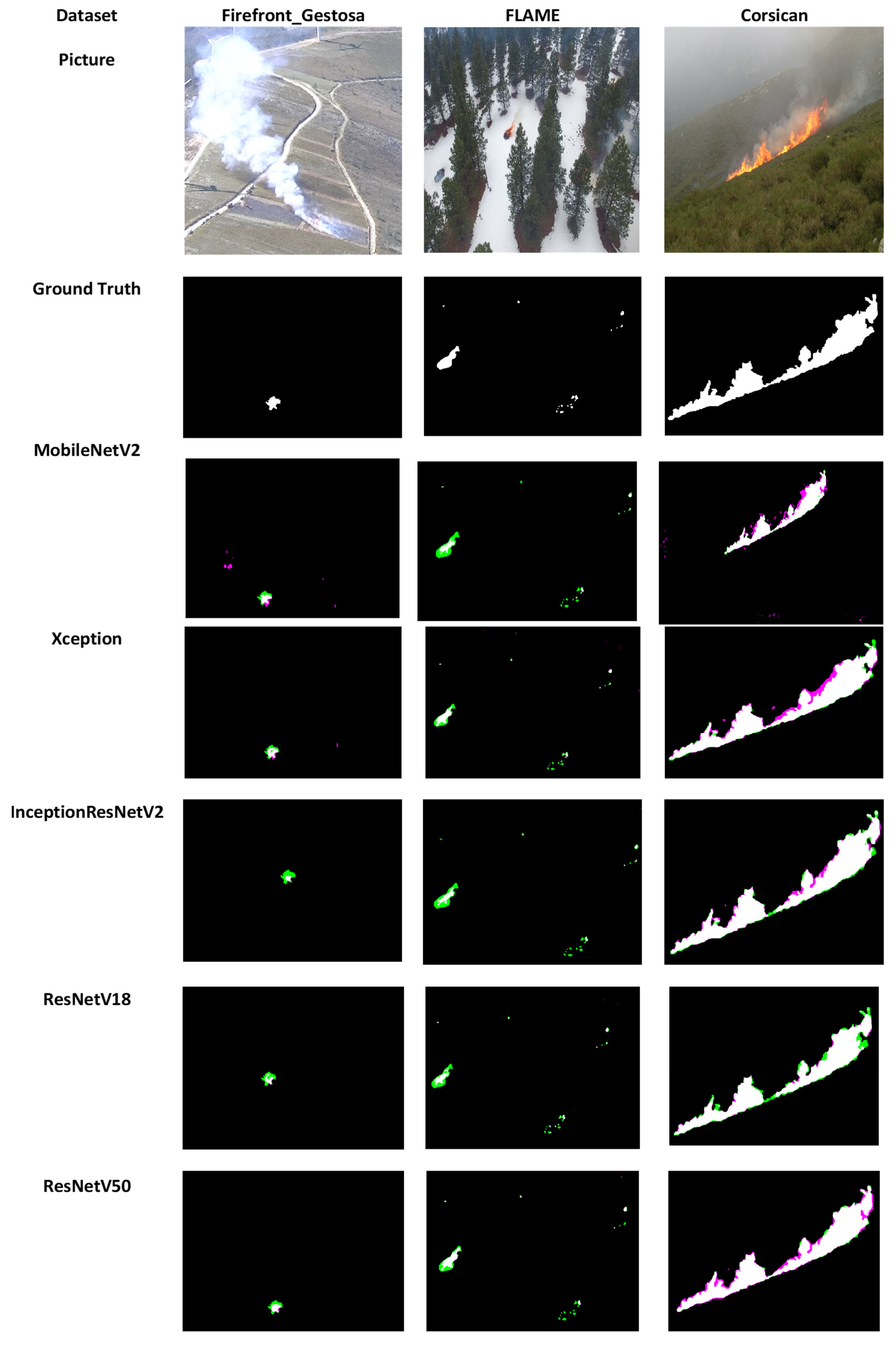
Model_5	98.65%	90.86%	86.27%	97.44%	93.63%

shows the overall performance of the five selected models while

Table 6. Computational cost of the five previously selected models: Average values of training time per network and detection time per image per dataset. We note that we had averaged the results of five repetitions.

Model	Average Training Time per Network (Hour:Minute:Second)	Average Detection Time per Image (Second)
		FLAME	Corsican	Firefont_Gestosa
Model_1	00:55:10	1.0181	0.6178	0.8745
Model_2	00:47:21	1.2033	0.68	1.0016
Model_3	01:29:20	7.0613	2.4511	4.9538
Model_4	00:47:59	0.9122	0.8375	0.7407
Model_5	01:05:34	1.1677	0.6459	1.0029

introduces the computational cost of every model in terms of training and test time per dataset.

It can be observed from the overall results depicted in Table 5 that ResNet-50 (Model_5) achieves the best performance with a global accuracy of 98.65%, a mean accuracy of 90.86%, a mean IoU 86.27%, a weighted IoU of 97.44%, and a mean BF score of 93.63%.

MobileNetV2 (Model_1) attains competitive performance, with a smaller training duration (average training time 55 min and 10 s), as shown in Table 6, in comparison with ResNet-50 (Model_5). Model_5 draws a global accuracy of 98.70%, a mean accuracy of 89.54%, a mean IoU 86.38%, a weighted IoU of 97.51%, and a mean BF score of 93.86%. The ResNet-50 had required an average training time of 1 h, 5 min, and 34 s.

The InceptionResNetV2 (Model_3) and the Xception (Model_2) architectures draw relatively lower performance since the first focuses on computational cost and the second, as an extension of the first, reframes the same network concept.

It is worth noting that the Xception substitutes the original Inception modules with depth-wise separable convolutions. InceptionResNetV2, as expected, required maximum training time (average 1 h, 29 min, and 20 s) as it is one of the most in-depth networks used in our study.

We note that it is normal that the average detection time over Firefront_Gestosa is relatively higher since the size of original images is bigger than FLAME and Corsican.

The performance of first and fifth models are highlighted in

Table 7. The observed metrics over every set of data for Model_1 and Model_5.

Model	Dataset	Global Accuracy	Mean Accuracy	Mean IoU	Weighted IoU	Mean BF Score
Model_1	FLAME	99.80%	87.81%	84.32%	99.62%	95.66%
	Corsican	97.30%	89.46%	85.76%	94.83%	91.21%
	Firefront_Gestosa	99.98%	89.01%	80.13%	99.96%	98.39%
Model_5	FLAME	99.79%	92.02%	84.74%	99.61%	96.43%
	Corsican	97.18%	90.49%	85.60%	94.69%	89.81%
	Firefront_Gestosa	99.97%	92.61%	79.09%	99.95%	98.60%

for better insight. It is evident that the Model_5 outperforms Model_1 based on performance comparison. The Model_5 draws higher results over Flame data, a global accuracy of 99.79%, a mean accuracy of 92.02% a mean IoU 84.74%, a weighted IoU of 99.61%, and a mean BF score of 96.43%. Alongside, Model_1 draws a very low mean accuracy and mean BF score of 87.81% and 95.66% respectively, in comparison to Model_5.

However, Model_5 attains a global accuracy of 99.97%, a mean accuracy of 92.61%, a mean IoU 79.09%, a weighted IoU of 99.95%, and a mean BF score of 98.60% over Firefront_Gestosa. Besides, Model_1 attains a higher mean IoU of 80,13% but a very low mean accuracy of 89.01% compared to Model_5. For the case of Corsican data, the Model_1 gives a higher mean Bf score.

Nonetheless, the computational cost of Model_5 is higher than Model_1. Notwithstanding that Model_5 consumes higher training resources; the detection time is the same as Model_1 (please refer to Table 6).

4.2.3. Test Samples

For example, the pictures in the third and seventh rows of the Figure 12 manifest extensively enhanced segmentation. The MobilenetV2 and ResNet-50 give finer boundary and more perfectly drawn flame shapes. Nonetheless, the corresponding results in the fourth, fifth, sixth rows demonstrate coarse and inaccurate boundaries, imprecise flame shapes, and more FNs (pixels drawn in pink).

4.3. State-of-the-Art Comparison

An accurate comparison of the results is challenging since the same training parameters, and validation modalities are used, even if the authors are using the same data, but evidentially not the same partition and metrics for evaluation.

For Corsican data, we had regrouped in the

Table 8. Resume of the state-of-art, mainly the algorithms tested over FLAME and Corsican datasets: comparison with the current work.

Algorithm Reference	Approach	Dataset	Global Accuracy	Mean Accuracy (Recall)	Mean IoU	Weighted IoU	Mean BF Score (F1 Score)
[11]	UNET	FLAME	99%	83.88%	78.17%	___	87.75%
Proposed approach	Deeplabv3+ with ResNet-50 backbone and Dice loss function		99.79%	92.02%	84.74%	99.61%	96.43%
[49]	Custom CNN residual network	Corsican	97.46%	95.17%	90.02%	___	94.70%
[48]	Deep–Fire U-Net		94.39%	88.78%	82.32%	___	89.48%
[36]	Deeplab		96.92%	90.42%	86.96%	___	92.69%
[51]	Color segmentation with fuzzy criteria		92.74%	75.10%	72.53%	___	80.04%
[24]	bee colony algorithm-based color space segmentation		___	___	76%	___	___
[50]	Custom CNN architecture		98.02%	___	___	92.53%	___
[52]	Weakly supervised CNN		___	___	72.86%	___	___
Proposed approach	Deeplabv3+ with ResNet-50 backbone and Dice loss function		97.18%	90.49%	85.60%	94.69%	89.81%
Proposed approach	Deeplabv3+ with ResNet-50 backbone and Dice loss function	Firefront_Gestosa	99.97%	92.61%	79.09%	99.95%	98.60%

the most outstanding studies and their corresponding announced results. Our model trained with ResNet-50 and Dice loss outperforms the Deep–Fire U-Net [48], CNN residual network [49], Deeplab [36], Custom CNN architecture [50], and the color segmentation approach with fuzzy criteria [51]. Nevertheless, for bee colony algorithm-based color space segmentation [24] and the weakly supervised CNN [52], it is quite difficult to judge following the few represented results.

Custom CNN residual network [49] outperforms our results, but it seems that no cross-validation was performed, just a single run result that could not be quite accurate. The FLAME dataset is newly released, so the work done is limited to the original dataset. It is clear from Table 8 that the present work model outperforms the UNet approach [11]. Moreover, no work was recorded using Firefront_Gestosa Videos or images, since it is private content. But the results are encouraging regarding the fact that the model is not concepted for this data specifically.

We note however, that in Table 8 some cells do not present results since the original works do not use the same metrics that have been adopted in this work.

5. Conclusions

In the past decades, the number of wildfires has increased while the available material and human capacities to fight them are still limited. Hence the response capacity must be optimized to avoid time and logistic loss due to false alarms. Various intelligent systems, namely artificial intelligence models, concepted to detect and localize fire zones are proposed. Few tendencies to work over aerial datasets make the segmentation process challenging due to the lack of fire pixels. The current system draws very encouraging results over a minor set of aerial fire images.

To conclude, the selected model trained with ResNet-50 and Dice loss attains a global accuracy of 98.70%, a mean accuracy of 89.54%, a mean IoU 86.38%, a weighted IoU of 97.51%, and a mean BF score of 93.86%. The computational cost is moderated. Nevertheless, the trained model could be used for segmentation of more similar aerial pictures that the manual segmentation is challenging and time consuming since it requires an affine level of precision.

The used aerial images are considered as limited set of data, since the number of pixels labeled as fire are less than usual. Hence, we had reinforced the dataset with Corsican pictures that have a frontal view of fire. The Firefront_Gestosa is private limited content. A performance analysis as functions of the training samples ratio could be conducted, however that would be more suited with a larger dataset. So, it will be considered in future work. Moreover, we will consider a bigger labeled set of Firefront_Gestosa pictures.

References

1. Global Forest Watch. Available online: https://www.globalforestwatch.org/ (accessed on 7 February 2022).
2. Libonati, R.; Geirinhas, J.L.; Silva, P.S.; Russo, A.; Rodrigues, J.A.; Belém, L.B.; Nogueira, J.; Roque, F.O.; DaCamara, C.C.; Nunes, A.M. Assessing the role of compound drought and heatwave events on unprecedented 2020 wildfires in the Pantanal. Environ. Res. Lett. 2022, 17, 015005. [Google Scholar] [CrossRef]
3. Mansoor, S.; Farooq, I.; Kachroo, M.M.; Mahmoud, A.E.D.; Fawzy, M.; Popescu, S.M.; Alyemeni, M.; Sonne, C.; Rinklebe, J.; Ahmad, P. Elevation in wildfire frequencies with respect to the climate change. J. Environ. Manag. 2022, 301, 113769. [Google Scholar] [CrossRef] [PubMed]
4. Rego, F.C.; Silva, J.S. Wildfires and landscape dynamics in Portugal: A regional assessment and global implications. In Forest Landscapes and Global Change; Springer: Berlin/Heidelberg, Germany, 2014; pp. 51–73. [Google Scholar]
5. Oliveira, S.; Gonçalves, A.; Zêzere, J.L. Reassessing wildfire susceptibility and hazard for mainland Portugal. Sci. Total Environ. 2021, 762, 143121. [Google Scholar] [CrossRef] [PubMed]
6. Ferreira-Leite, F.; Ganho, N.; Bento-Gonçalves, A.; Botelho, F. Iberian atmospheric dynamics and large forest fires in mainland Portugal. Agric. For. Meteorol. 2017, 247, 551–559. [Google Scholar] [CrossRef]
7. Costa, L.; Thonicke, K.; Poulter, B.; Badeck, F.-W. Sensitivity of Portuguese forest fires to climatic, human, and landscape variables: Subnational differences between fire drivers in extreme fire years and decadal averages. Reg. Environ. Chang. 2011, 11, 543–551. [Google Scholar] [CrossRef]
8. Yuan, C.; Liu, Z.; Zhang, Y. Vision-based forest fire detection in aerial images for firefighting using UAVs. In Proceedings of the 2016 International Conference on Unmanned Aircraft Systems (ICUAS), Arlington, VA, USA, 7–10 June 2016; pp. 1200–1205. [Google Scholar]
9. Chen, L.-C.; Zhu, Y.; Papandreou, G.; Schroff, F.; Adam, H. Encoder-decoder with atrous separable convolution for semantic image segmentation. In Proceedings of the European Conference on Computer Vision (ECCV), Munich, Germany, 8–14 September 2018; pp. 801–818. [Google Scholar]
10. Toulouse, T.; Rossi, L.; Campana, A.; Celik, T.; Akhloufi, M.A. Computer vision for wildfire research: An evolving image dataset for processing and analysis. Fire Saf. J. 2017, 92, 188–194. [Google Scholar] [CrossRef] [Green Version]
11. Shamsoshoara, A.; Afghah, F.; Razi, A.; Zheng, L.; Fulé, P.Z.; Blasch, E. Aerial Imagery Pile burn detection using Deep Learning: The FLAME dataset. Comput. Netw. 2021, 193, 108001. [Google Scholar] [CrossRef]
12. Blalack, T.; Ellis, D.; Long, M.; Brown, C.; Kemp, R.; Khan, M. Low-Power Distributed Sensor Network for Wildfire Detection. In Proceedings of the 2019 SoutheastCon, Huntsville, AL, USA, 11–14 April 2019; pp. 1–3. [Google Scholar]
13. Brito, T.; Pereira, A.I.; Lima, J.; Valente, A. Wireless sensor network for ignitions detection: An IoT approach. Electronics 2020, 9, 893. [Google Scholar] [CrossRef]
14. Veraverbeke, S.; Dennison, P.; Gitas, I.; Hulley, G.; Kalashnikova, O.; Katagis, T.; Kuai, L.; Meng, R.; Roberts, D.; Stavros, N. Hyperspectral remote sensing of fire: State-of-the-art and future perspectives. Remote Sens. Environ. 2018, 216, 105–121. [Google Scholar] [CrossRef]
15. Dennison, P.E.; Roberts, D.A.; Kammer, L. Wildfire detection for retrieving fire temperature from hyperspectral data. J. Sci. Eng. Res. 2017, 4, 126–133. [Google Scholar]
16. Toan, N.T.; Cong, P.T.; Hung, N.Q.V.; Jo, J. A deep learning approach for early wildfire detection from hyperspectral satellite images. In Proceedings of the 2019 7th International Conference on Robot Intelligence Technology and Applications (RiTA), Daejeon, Korea, 1–3 November 2019; pp. 38–45. [Google Scholar]
17. Liu, C.; Xing, C.; Hu, Q.; Wang, S.; Zhao, S.; Gao, M. Stereoscopic hyperspectral remote sensing of the atmospheric environment: Innovation and prospects. Earth-Sci. Rev. 2022, 226, 103958. [Google Scholar] [CrossRef]
18. Mei, S.; Geng, Y.; Hou, J.; Du, Q. Learning hyperspectral images from RGB images via a coarse-to-fine CNN. Sci. China Inf. Sci. 2022, 65, 1–14. [Google Scholar] [CrossRef]
19. Yuan, C.; Zhang, Y.; Liu, Z. A survey on technologies for automatic forest fire monitoring, detection, and fighting using unmanned aerial vehicles and remote sensing techniques. Can. J. For. Res. 2015, 45, 783–792. [Google Scholar] [CrossRef]
20. Sudhakar, S.; Vijayakumar, V.; Kumar, C.S.; Priya, V.; Ravi, L.; Subramaniyaswamy, V. Unmanned Aerial Vehicle (UAV) based Forest Fire Detection and monitoring for reducing false alarms in forest-fires. Comput. Commun. 2020, 149, 1–16. [Google Scholar] [CrossRef]
21. Badiger, V.; Bhalerao, S.; Mankar, A.; Nimbalkar, A. Wireless Sensor Network-Assisted Forest Fire Detection and Control Firefighting Robot. SAMRIDDHI J. Phys. Sci. Eng. Technol. 2020, 12, 50–57. [Google Scholar]
22. Vani, K. Deep learning based forest fire classification and detection in satellite images. In Proceedings of the 2019 11th International Conference on Advanced Computing (ICoAC), Chennai, India, 18–20 December 2019; pp. 61–65. [Google Scholar]
23. Toulouse, T.; Rossi, L.; Akhloufi, M.; Celik, T.; Maldague, X. Benchmarking of wildland fire colour segmentation algorithms. IET Image Process. 2015, 9, 1064–1072. [Google Scholar] [CrossRef] [Green Version]
24. Toptaş, B.; Hanbay, D. A new artificial bee colony algorithm-based color space for fire/flame detection. Soft Comput. 2019. [Google Scholar] [CrossRef]
25. Toulouse, T.; Rossi, L.; Akhloufi, M.A.; Pieri, A.; Maldague, X. A multimodal 3D framework for fire characteristics estimation. Meas. Sci. Technol. 2018, 29, 025404. [Google Scholar] [CrossRef]
26. Cheng, S.; Ma, J.; Zhang, S. Smoke detection and trend prediction method based on Deeplabv3+ and generative adversarial network. J. Electron. Imaging 2019, 28, 033006. [Google Scholar] [CrossRef]
27. Frizzi, S.; Kaabi, R.; Bouchouicha, M.; Ginoux, J.; Moreau, E.; Fnaiech, F. Convolutional neural network for video fire and smoke detection. In Proceedings of the IECON 2016—42nd Annual Conference of the IEEE Industrial Electronics Society, Florence, Italy, 23–26 October 2016; pp. 877–882. [Google Scholar]
28. Jia, Y.; Yuan, J.; Wang, J.; Fang, J.; Zhang, Q.; Zhang, Y. A Saliency-Based Method for Early Smoke Detection in Video Sequences. Fire Technol. 2016, 52, 1271–1292. [Google Scholar] [CrossRef]
29. Nemalidinne, S.M.; Gupta, D. Nonsubsampled contourlet domain visible and infrared image fusion framework for fire detection using pulse coupled neural network and spatial fuzzy clustering. Fire Saf. J. 2018, 101, 84–101. [Google Scholar] [CrossRef]
30. Yuan, F.; Zhang, L.; Xia, X.; Huang, Q.; Li, X. A Gated Recurrent Network With Dual Classification Assistance for Smoke Semantic Segmentation. IEEE Trans. Image Process. 2021, 30, 4409–4422. [Google Scholar] [CrossRef] [PubMed]
31. Mahmoud, M.A.I.; Ren, H. Forest fire detection and identification using image processing and SVM. J. Inf. Process. Syst. 2019, 15, 159–168. [Google Scholar]
32. Yuan, C.; Liu, Z.; Zhang, Y. UAV-based forest fire detection and tracking using image processing techniques. In Proceedings of the 2015 International Conference on Unmanned Aircraft Systems (ICUAS), Denver, CO, USA, 9–12 June 2015; pp. 639–643. [Google Scholar]
33. Guede-Fernández, F.; Martins, L.; Almeida, R.V.d.; Gamboa, H.; Vieira, P. A deep learning based object identification system for forest fire detection. Fire 2021, 4, 75. [Google Scholar] [CrossRef]
34. Zhao, Y.; Ma, J.; Li, X.; Zhang, J. Saliency detection and deep learning-based wildfire identification in UAV imagery. Sensors 2018, 18, 712. [Google Scholar] [CrossRef] [PubMed] [Green Version]
35. Song, K.; Choi, H.-S.; Kang, M. Squeezed fire binary segmentation model using convolutional neural network for outdoor images on embedded device. Mach. Vis. Appl. 2021, 32, 120. [Google Scholar] [CrossRef]
36. Mlích, J.; Koplík, K.; Hradiš, M.; Zemčík, P. Fire Segmentation in Still Images. In Proceedings of the Advanced Concepts for Intelligent Vision Systems, Auckland, New Zealand, 10–14 February 2020; pp. 27–37. [Google Scholar]
37. Available online: http://firefront.pt/ (accessed on 7 February 2022).
38. Thomas, S.W. Efficient inverse color map computation. In Graphics Gems II; Elsevier: Amsterdam, The Netherlands, 1991; pp. 116–125. [Google Scholar]
39. He, K.; Zhang, X.; Ren, S.; Sun, J. Deep Residual Learning for Image Recognition. In Proceedings of the 2016 IEEE Conference on Computer Vision and Pattern Recognition (CVPR), Honolulu, HI, USA, 21–26 July 2016; pp. 770–778. [Google Scholar]
40. He, K.; Zhang, X.; Ren, S.; Sun, J. Identity mappings in deep residual networks. In Proceedings of the European Conference on Computer Vision, Amsterdam, The Netherlands, 11–14 October 2016; pp. 630–645. [Google Scholar]
41. Sandler, M.; Howard, A.; Zhu, M.; Zhmoginov, A.; Chen, L.-C. Mobilenetv2: Inverted residuals and linear bottlenecks. In Proceedings of the IEEE Conference on Computer Vision and Pattern Recognition, Salt Lake City, UT, USA, 18–22 June 2018; pp. 4510–4520. [Google Scholar]
42. Chollet, F. Xception: Deep learning with depthwise separable convolutions. In Proceedings of the IEEE Conference on Computer Vision and Pattern Recognition, Honolulu, HI, USA, 21–26 July 2017; pp. 1251–1258. [Google Scholar]
43. Szegedy, C.; Ioffe, S.; Vanhoucke, V.; Alemi, A.A. Inception-v4, inception-resnet and the impact of residual connections on learning. In Proceedings of the Thirty-First AAAI Conference on artificial Intelligence, San Francisco, CA, USA, 4–9 February 2017. [Google Scholar]
44. Sudre, C.H.; Li, W.; Vercauteren, T.; Ourselin, S.; Cardoso, M.J. Generalised dice overlap as a deep learning loss function for highly unbalanced segmentations. In Deep Learning in Medical Image Analysis and Multimodal Learning for Clinical Decision Support; Springer: Berlin/Heidelberg, Germany, 2017; pp. 240–248. [Google Scholar]
45. Salehi, S.S.M.; Erdogmus, D.; Gholipour, A. Tversky loss function for image segmentation using 3D fully convolutional deep networks. In Proceedings of the International Workshop on Machine Learning in Medical Imaging, Quebec City, QC, Canada, 10 September 2017; pp. 379–387. [Google Scholar]
46. Yin, T.; Goyal, P.; Girshick, R.; He, K.; Dollár, P. Focal loss for dense object detection. In Proceedings of the IEEE International Conference on Computer Vision, Venice, Italy, 22–29 October 2017; pp. 2999–3007. [Google Scholar]
47. Ma, Y.-D.; Liu, Q.; Qian, Z.-B. Automated image segmentation using improved PCNN model based on cross-entropy. In Proceedings of the 2004 International Symposium on Intelligent Multimedia, Video and Speech Processing, Hong Kong, China, 20–22 October 2004; pp. 743–746. [Google Scholar]
48. Akhloufi, M.A.; Tokime, R.B.; Elassady, H. Wildland fires detection and segmentation using deep learning. In Proceedings of the Pattern Recognition and Tracking xxix, Orlando, FL, USA, 18–19 April 2018; p. 106490B. [Google Scholar]
49. Choi, H.-S.; Jeon, M.; Song, K.; Kang, M. Semantic Fire Segmentation Model Based on Convolutional Neural Network for Outdoor Image. Fire Technol. 2021, 57, 3005–3019. [Google Scholar] [CrossRef]
50. Niknejad, M.; Bernardino, A. Attention on Classification for Fire Segmentation. arXiv 2021, arXiv:2111.03129. [Google Scholar]
51. Dzigal, D.; Akagic, A.; Buza, E.; Brdjanin, A.; Dardagan, N. Forest Fire Detection based on Color Spaces Combination. In Proceedings of the 2019 11th International Conference on Electrical and Electronics Engineering (ELECO), Bursa, Turkey, 28–30 November 2019; pp. 595–599. [Google Scholar]
52. Niknejad, M.; Bernardino, A. Weakly-supervised fire segmentation by visualizing intermediate CNN layers. arXiv 2021, arXiv:2111.08401. [Google Scholar]
Figure 1. The proposed framework for fire detection. First, the dataset is labeled and correctly formatted; later, the model is trained to locate the flames. Then the deeplabv3+ model is used to generate the segmentation mask.
Remotesensing 14 02023 g001
Figure 2. Examples of fire pictures are included in our simulation dataset: (a) Multimodal, (b) RGB spectra, (c) IR spectra pictures taken from the Corsican dataset. (d) RGB pictures from FLAME dataset, (e) pictures from Firefront_Gestosa.
Remotesensing 14 02023 g002
Figure 3. The segmentation module architecture: The encoder block is for feature extraction, deploying atrous convolutions with different rates (spatial pyramid pooling block). The decoder block helps reduce the obtained feature map.
Remotesensing 14 02023 g003
Figure 4. The overall metrics were gathered using different loss functions with Deeplabv3+ with MobileNetV2 as the backbone.
Remotesensing 14 02023 g004
Figure 5. The overall metrics were gathered using different loss functions with Deeplabv3+ with Xception as the backbone.
Remotesensing 14 02023 g005
Figure 6. The overall metrics were gathered using different loss functions with Deeplabv3+ with InceptionResNetV2 as a backbone.
Remotesensing 14 02023 g006
Figure 7. The overall metrics, over the three sets of data (FLAME, Corsican, and Firefront_Gestosa), gathered using Tversky and Dice loss functions with Deeplabv3+ with InceptionResNetV2 as backbone.
Remotesensing 14 02023 g007
Figure 8. The overall metrics were gathered using different loss functions with Deeplabv3+ with ResNet-18 as a backbone.
Remotesensing 14 02023 g008
Figure 9. The overall metrics, over the three sets of data (FLAME, Corsican, and Firefront_Gestosa), were gathered using Cross entropy and Dice loss functions with Deeplabv3+ with ResNet-18 as a backbone.
Remotesensing 14 02023 g009
Figure 10. The overall metrics gathered using different loss function with Deeplabv3+ with ResNet-50 as backbone.
Remotesensing 14 02023 g010
Figure 11. The overall metrics, over the three sets of data (FLAME, Corsican, and Firefront_Gestosa), were gathered using Tversky and Dice loss functions with Deeplabv3+ with ResNet-50 as a backbone.
Remotesensing 14 02023 g011
Figure 12. Example of segmentation of a picture of every dataset: The first, second, and third columns are result examples from Firefront_Gestosa, FLAME, and Corsican data, respectively. The first and second rows are the pictures and their corresponding ground truths. The rows from three to seven represent the results given by the four models trained with dice loss. The pixels that should be detected as non-fire, but the model had labeled them as fire pixels (FP), are given in green color. Pink color design pixels that are fire ones, but the model had labeled them as non-fire pixels (FN).
Remotesensing 14 02023 g012