ST-PN: A Spatial Transformed Prototypical Network for Few-Shot SAR Image Classification

Abstract

Few-shot learning has achieved great success in computer vision. However, when applied to Synthetic Aperture Radar Automatic Target Recognition (SAR-ATR), it tends to demonstrate a bad performance due to the ignorance of the differences between SAR images and optical ones. What is more, the same transformation on both images may cause different results, even some unexpected noise. In this paper, we propose an improved Prototypical Network (PN) based on Spatial Transformation, also known as ST-PN. Cascaded after the last convolutional layer, a spatial transformer module implements a feature-wise alignment rather than a pixel-wise one, so more semantic information can be exploited. In addition, there is always a huge divergence even for the same target when it comes to pixel-wise alignment. Moreover, it reduces computational cost with fewer parameters of the deeper layer. Here, a rotation transformation is used to reduce the discrepancies caused by different observation angles of the same class. Thefinal comparison of four extra losses indicates that a single cross-entropy loss is good enough to calculate the loss of distances. Our work achieves state-of-the-art performance on the Moving and Stationary Target Acquisition and Recognition (MSTAR) dataset.

1. Introduction

Synthetic Aperture Radar (SAR) provides sample information of the ground surface in all weather and time circumstances. Recently, SAR-ATR has attracted more and more attention with the fast development of space technology and deep learning. Thanks to its ability to process a large amount of data, a lot of deep learning methods have been used in SAR-ATR problems [1]. As an effective way of obtaining information of the ground surface, SAR-ATR has been widely applied in GIS system research, military reconnaissance, environmental monitoring, geological exploration, and so on.

However, as the quality of SAR images becomes better and better, the cost of acquiring images does not decrease accordingly, making it hard to obtain enough images. In addition, due to the sampling strategy of SAR, it is hard to ensure that the sampled regions and targets are uniformly distributed. So, there is always an unbalanced problem in different classes of samples. This brings a huge challenge to SAR-ATR tasks. In optical image processing, there is an effective way to handle this, which is called Few-Shot Learning (FSL) [2]. FSL is a branch of machine learning which is specialized in learning with limited supervised information. The lack of real samples accelerates its booming. Up to now, the existing few-shot learning algorithms either try to connect to extra large-scale datasets with strong correlations [3] or use specific measurements to represent the mapping relationships between samples [4]. Yet, this kind of dataset may not always exist, and average measurements are just too simple to represent the complicated mapping relationships explicitly enough, thus making few-shot learning a tough subject to explore.

To improve the performance of few-shot learning algorithms, a lot of work has been conducted [5].

Table 1. Existing methods of few-shot learning.

Category	Methods	Brief Description
Data-based	supervision	azimuth, size, area of shadow, etc.
	augmentation	geometric transformation
	generalization	from external highly correlated dataset
Model-based	metric learning	mapping images into lower-dimensional space
	external memory	to store learned information
	fine-tuning	fine-tuning pre-trained parameters
	meta-learning	for better initialization parameters

shows a summarization of these methods. First, from the image itself, some have tried to teach a classifier under the supervision of different azimuths, sizes, or areas of shadow, etc. [6,7,8,9,10]. However, due to the different observation angles, there could be parts covered with shadows, which results in black zones in an image. This increases the intra-class difference, making it even harder to extract invariant features. Another attempt is to enlarge the previous datasets using data augmentation [11,12,13]. Either learning a set of geometric transformations [14,15] or generating samples from other highly correlated datasets could alleviate the shortage of data to a great extent. Still, this kind of method can only work for some specific datasets, and different datasets usually follow different augmentation strategies.

In terms of model improvements, there exist several other methods. First of all, metric learning [16,17,18] maps an image into a lower-dimensional space with more distinguishability, where intra-class samples become closer while inter-class samples become further away from each other. Considering the limitation of the capacity of a model, some try to introduce external memory to store the mapping relationships between samples [19,20]. We can simply perform a weighted average on the contents extracted from the memory to represent a novel one. However, this external memory often has a limited capacity. So, we have to give up some existing values when it is out of memory. What is more, fine-tuning methods provide a way to fine-tune pre-trained parameters with the supervision of the current dataset. Again, overfitting is more likely in auxiliary datasets, causing a lack of generalization ability in new categories. To better learn the task-generic information among datasets, meta-learning is also an excellent way to refine a better group of initialization parameters [21,22]. This method could avoid falling into a local minimum to a great extent. Still, a precision sacrifice for speed and huge computation cost due to extensive use of second derivative calculation is the main drawback.

To minimize the complexity of the learning procedure and to reduce the number of additional images included, a metric learning algorithm named Prototypical Network (PN) was proposed by Snell in 2017 [23]. While taking a four-layer CNN as the backbone [24], PN learns a metric space in which classification can be performed by simply computing their Euclidean distances to the class prototypes. PN gives better performance while adopting a simpler inductive inference within this limited-data regime. However, CNN does not possess spatial invariance, making Euclidean distance a bit less meaningful [25]. Moreover, the mapping space is not bound to be separable, leading to lower performance on the current dataset [26].

To solve all these above problems, we propose an improved Prototypical Network based on a spatial transformer here. Taking a four-layer CNN as the backbone, a spatial transformer module is then included to perform an affine transformation on the extracted features. Spatial alignment is achieved during the modification of loss backpropagation. To summarize our efforts as follows:

• An extra Spatial Transformer Network (STN) is employed as a module to achieve spatial alignment on features derived from a CNN-based feature extractor, since CNN cannot extract features with invariance [27]. STN makes this learning process more explicit.
• We have conducted several experiments on the location, structure, and transformation type of STN and found out that a feature-wise alignment is better than a pixel-wise one. In addition, rotation outperforms all the other affine transformations.
• We have also conducted several experiments on loss function and found out that a simple Cross-Entropy loss fits the best.

2. Related Work

Inspired by the human ability to learn new things fast from one simple demonstration, few-shot learning tries to achieve the same thing. Like all other machine learning applications, there are usually two stages in a typical FSL procedure: the training and testing stages. Accordingly, there are training sets and testing sets. Usually, there is no overlap between these two parts. While all samples used in the training set are labeled, only a small part of samples in the testing set are labeled, which is known as the support set. Then, the rest of the unlabeled samples are used as the query set. FSL aims to obtain good learning performance given the limited information of the support set.

Figure 1 shows the whole learning procedure. To simulate the circumstance of the testing stage where labeled samples are rare, a sampling strategy is applied in the training stage. N classes are randomly selected first in the training set. Then, K samples are sampled from each class to form the support set. Meanwhile, Q samples are randomly selected from the rest of each class to form the query set. There is the same operation in the testing set. We call it an N-way K-shot problem when there are K samples from each of the C classes in the support set.

2.1. Few-Shot Learning

Few-shot learning tries to figure out the similarity between query sets and support sets before classification. All the existing methods can be roughly categorized into four types, that is, meta-learning, fine-tuning, metric learning, and external-memory-based methods. Meta-learning is also known as learning to learn. Instead of learning the task-specific parameters directly, meta-learning exploits the intrinsic meta-knowledge through the learning process of training several tasks to obtain the ability to adapt to new tasks as fast as possible [28]. The learner for a specific task is called a base-learner, and the meta-knowledge learner is called a meta-learner [22]. The most commonly used models are Model-Agnostic Meta-Learning (MAML) proposed by Chelsea Finn et al. in 2017 [29] and Reptile proposed by Nichol et al. in 2018 [30]. Both are used to obtain a set of initialization parameters that can make the network converge quickly using only a few samples. What is different between them is that MAML uses the average loss on testing sets of each base-learner to update the parameters of the meta-learner after all tasks are executed. In contrast, Reptile takes the latest after performing K training episodes for each specific task.

Fine-tuning methods pre-train the model on extra large-scale datasets before fine-tuning with a small amount of new labeled samples. Instead of optimizing from scratch, the backbone is first pre-trained for a faster as well as better convergence [31].

External-memory-based methods learn meta-knowledge from training sets and store it in external memories. Each new sample is then classified depending on its weighted relationship with the memory contents. However, as the capacity of a memory module is usually finite, even with a lifelong memory [32], some older and rare slots can still be forgotten and removed.

The last method is metric learning. This approach uses a simple CNN structure to extract features from input images. Then, a distance classifier is appended to compute similarity among seen and unseen classes. A Siamese Network [33] is a basic but representative architecture that compares the similarity between input embeddings. Inspired by the attention mechanism and external memory, the Matching Network [34] and Cross Attention Network (CAN) [26] are proposed to further explore semantic correlations between seen and unseen classes. The Prototypical Network [23] aims to reduce the computational cost, and the Relation Network [35] intends to represent the complex mapping relationships via a neural network instead of Euclidean distance [36]. Another approach extends metrics from Euclidean space to manifold space [37].

2.2. Few-Shot SAR Image Classification via Metric Learning

While in SAR-ATR tasks, it is hard to ensure that data are uniformly sampled, and it takes considerable cost to obtain sufficient images. The application of FSL has been more and more common [5]. Among all the mainstream FSL methods, metric learning embeds samples to a lower-dimensional space, where similar samples are close to each other and dissimilar samples are far away from each other [5].

For improvements in the feature extractor, Wang et al. [38] noticed that it might not be appropriate to use Euclidean distance considering different azimuths of the same class. They introduced BiLSTM to extract the feature sequences of the target image rotated by 90°, 180° and 270°. Then, an average of the vectors was taken as the new feature of the target image. It has achieved a classification accuracy of more than 90%.

For loss enhancement, Tang et al. [39] improved the Siamese Network with a softmax classifier for each input, which improved the classification accuracy, accelerated the network convergence, and reduced GPU consumption. However, the main disadvantage is that the proportion of various losses is determined by experience and lacks interpretability. Lu et al. [40] was inspired by triple loss in face recognition and introduced it into FSL. Meanwhile, they used online learning to mine hard triples, which greatly improved the performance on the MSTAR dataset.

For manifold consideration, Rostami [41] and others considered mapping the optical image and SAR image to the shared space to minimize the difference in their distribution in the shared space. Encouraging results were obtained on the “EO Ships in Satellite Imagery” dataset. Wang et al. [42] considered that the existing methods generally determine the similarity between the query set and the support set according to certain rules. However, the support set is not necessarily representative. So, they included transductive inference together with inductive inference and a hybrid enhanced loss algorithm. Not only was the mapping relationship between query set and support set was considered, but also the manifold of query set was considered as well, which showed an excellent performance. Yang et al. [4] replaced the original fully connected layer by Graph Neural Network with an attention mechanism to better extract the mapping relationship between query and support samples. Thanks to its lightweight structure as well as independence on extra large-scale datasets, metric learning has been widely applied in SAR-ATR problems.

3. Materials and Methods

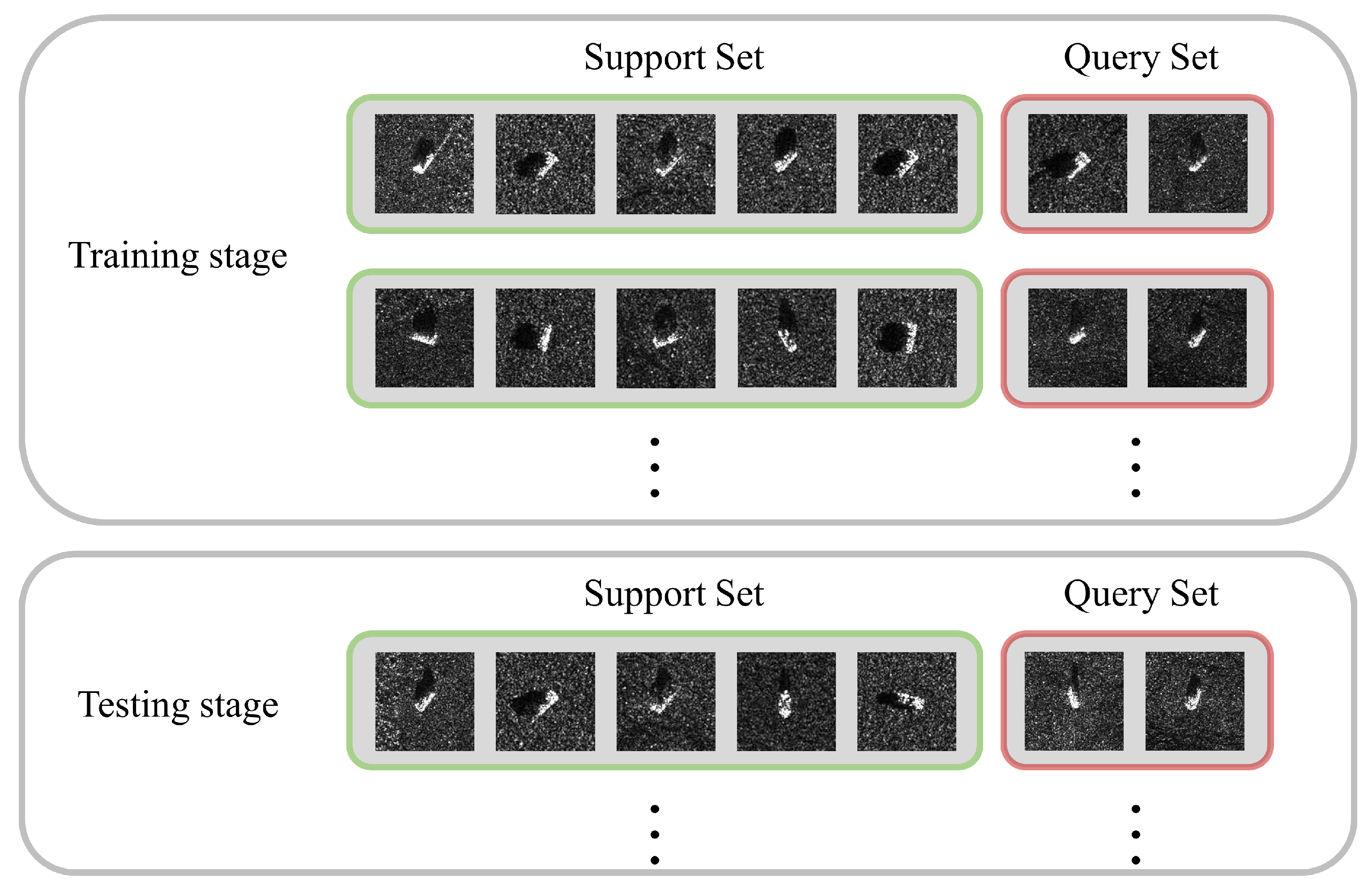
Few-shot classification tries to generalize to novel classes, given only a few samples of each class. Among all those mainstream methods, metric-based methods give excellent performance with independence on extra large-scale datasets [5]. Prototypical Network is one of the well-performed baselines by computing distances to the prototype embeddings of each class. Therefore, how to map the inputs into an appropriate embedding space becomes a crucial but challenging problem here.

The Prototypical Network maps inputs into a metric space using a four-layer CNN as the feature extractor. Taking the mean of a class’s embeddings as the class prototype, classification is then performed for a query embedding by simply categorizing it into the nearest class via the Euclidean distance. However, CNN can only keep the translation invariance of a local small range, not to mention the global invariance of scale or rotation. When it comes to inputs with multi-azimuth and multi-depression-angle, CNN usually cannot work well in obtaining features with good spatial invariance [27]. In addition, a support set is not bound to be representative in every training episode [26], thus making the Euclidean distance meaningless to some extent. Therefore, instead of letting the network learn invariant features automatically, our goal is to make this procedure more explicit and ensure that features of the same class are aligned when query set classification is conducted.

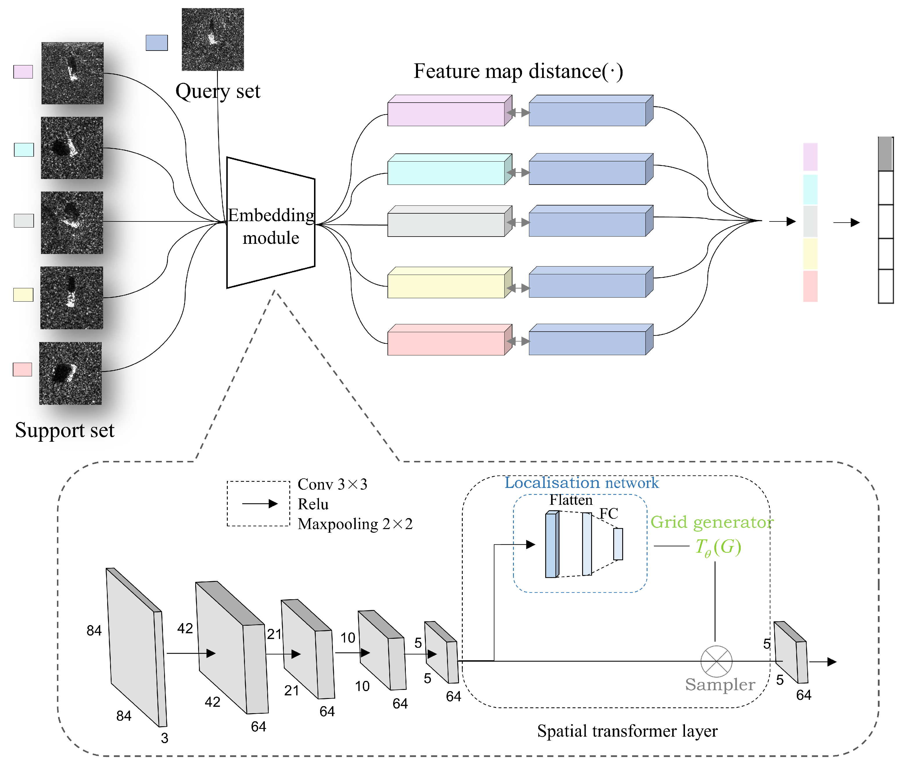
We solved this problem by proposing a novel Spatial-Transformer-based Prototypical Network, denoted as ST-PN. Figure 2 shows the overall architecture of our proposed ST-PN. An input image is embedded by the embedding module, which consists of a four-layer CNN and a spatial transformer module. Then, we use Euclidean distance to represent the similarity between one another and categorize it into the nearest class. A spatial transformer module is designed to achieve spatial alignment so that Euclidean distance makes more sense with better characteristics of invariance [27]. Moreover, Table 4 shows that a feature-wise alignment fits better than a pixel-wise one. Furthermore, more latent information is to be explored as the layer goes deeper. We employ a rotation transformation here to align samples from different azimuths. All these parts work together to give better performances on SAR image classification.

3.1. Spatial Transformer Module

A spatial transformer module tries to achieve spatial alignment to features extracted by CNN. These features either contain semantic information of higher-level or local detailed information of lower level. Prototypical Network takes mean of the class’ embeddings as prototypes, which contains azimuth information. That makes Euclidean distance meaningless due to the azimuth divergence. To better classify feature representations, spatial alignment is needed to alleviate this discrepancy.

A detailed structure of the embedding module is shown in the lower part of Figure 2. Feature embeddings are generated via 4 convolutional layers, each followed by a ReLU activation function and a max-pooling layer. After that, a spatial transformer module is included to implement the spatial alignment, which is formed by a localization network, a grid generator, and a sampler [27].

The localization network takes feature maps as input and outputs $\mathsf{\Theta }$, parameters to be applied to transform input feature maps. There are usually convolutional or fully connected layers in a localization network which ends with a regression layer for $\mathsf{\Theta }$. In detail, a 3 × 3 convolutional layer followed by a max-pooling layer and a ReLU function, appended with a fully connected layer is employed to regress the transformation parameters in localization network. While a convolutional layer attempts for semantic information of higher-level, a fully connected layer introduces more non-linearity to fit the complex mapping relationships between features and parameters. The input feature size must be the same as the output. Hence, to perform the feature mapping, the grid generator generates a corresponding sampling grid according to the input feature map. Then, a sampling operation is conducted to fill up the output feature map for each channel, mostly through bilinear interpolation. For when mapped into the output feature maps, the corresponding coordinates of pixels are not usually integers. Then, the surrounding pixels are needed when calculating their values.

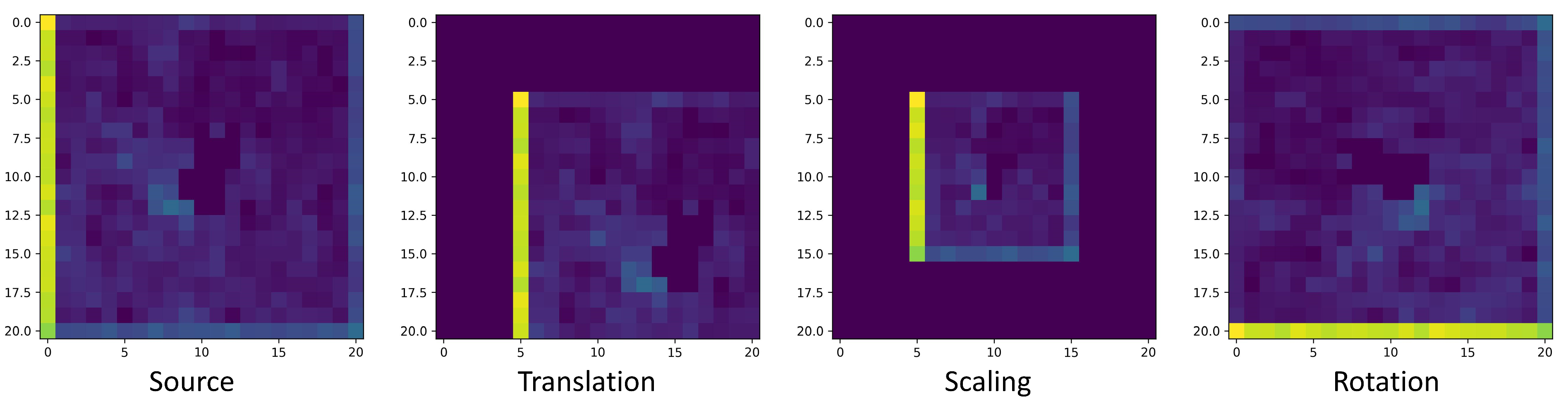
A simple affine transformation is used here in order to not bring in too many parameters and is also enough to represent most transformations of the 2D SAR images. Figure 3 shows some of the transformations.

Usually a point-wise affine transformation can be described as:

$$\left(\begin{array}{c}{x}_s\\ y_s\end{array}\right)=\mathsf{\Theta }\left(\begin{array}{c}{x}_t\\ y_t\\ 1\end{array}\right)=\left(\begin{array}{ccc}{\mathsf{\Theta }}_{11}& {\mathsf{\Theta }}_{12}& {\mathsf{\Theta }}_{13}\\ {\mathsf{\Theta }}_{21}& {\mathsf{\Theta }}_{22}& {\mathsf{\Theta }}_{23}\end{array}\right)\left(\begin{array}{c}{x}_t\\ y_t\\ 1\end{array}\right)$$

(1)

where $(x_s,y_s)$ denotes a source coordinate of the input, while $(x_t,y_t)$ denotes the corresponding target coordinate of the output. For example, $\mathsf{\Theta }$ for translation is denoted as $\left(\begin{array}{ccc}1& 0& d_s\\ 0& 1& d_y\end{array}\right)$, and $\left(\begin{array}{ccc}cos\theta & -sin\theta & 0\\ sin\theta & cos\theta & 0\end{array}\right)$ is for rotation.

3.2. CNN as Backbone

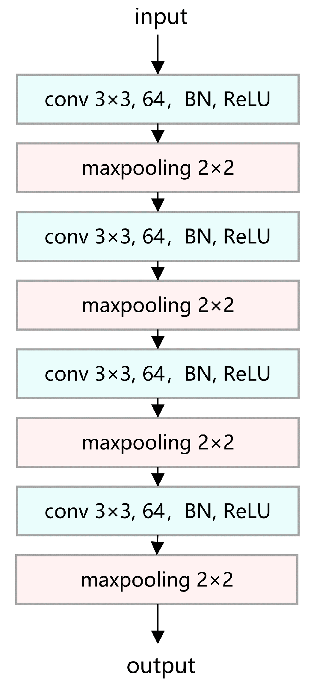
Extracting features from the input images could be an essential part of image processing. The whole backbone architecture is shown in Figure 4. There are four convolutional layers in this structure, each followed by a ReLU activation, a batch normalization, and a max-pooling layer. It maps the input images into a lower and more organized metric space. Here, we use a typical setting of 3 × 3 kernel of a convolutional layer to extract global features. Then, a max-pooling layer with a kernel of 2 × 2 is included to decrease the dimensions of features as well as maintain its information.

3.3. Prediction and Loss

Here, the SAR image classification can be described as an N-way K-shot problem as mentioned above. Let S be the support set where $S=\{S_1,S_2,\dots ,S_i,\dots ,S_N\}$. $S_i$ denotes the ith class of unseen classes. There are K labeled samples in each of the N classes in the support set, which is defined as $S_i=\{(x_{i1},y_{i1}),\dots ,(x_{ij},y_{ij}),(x_{ik},y_{ik})\}$. $y_{ij}$ stands for the corresponding class label of $x_{ij}$. Let the mapping function of the backbone be $f_{\theta }$, then the prototype for each class in the support set can be represented as:

$$c_i=\frac{1}{K}\sum _{(x_{ij},y_{ij})\in S_i}{f}_{\theta }(x_{ij})$$

(2)

The whole network is trained from scratch. Both the support set and query set are embedded via the same embedding module. Then, a Euclidean distance is calculated to measure the similarity between the query set and class prototypes. In detail, given feature vector q of an unlabeled image and $c_i$ as the prototype of the ith class, the similarity can be calculated as:

$$d(q,c_i)={\parallel q-c_i\parallel }_2^2$$

(3)

Then, a softmax function is adopted to measure it probability of belonging to the ith class:

$$P(y=n|q)=\frac{exp(-d(q,c_i))}{{\sum }_{i=1}^{N}exp(-d(q,c_i))}$$

(4)

Prediction of q depends on the maximum probability over N classes, which is denoted as:

$$y_q=\underset{n}{argmax}P(y=n|q)$$

(5)

An overall loss function of the proposed network is CrossEntropy loss, which is widely used in image classification problems.

4. Results

4.1. Datasets

To validate the effectiveness of the proposed ST-PN, our work is implemented on the Moving and Stationary Target Acquisition and Recognition (MSTAR) dataset. MSTAR is a public SAR image dataset released by Defense Advanced Research Projects Agency (DARPA), which has been used in thousands of SAR-ATR studies.

This dataset consists of 10 kinds of vehicles: 2S1, BMP2, BRDM2, BTR60, BTR70, D7, T62, T72, ZIL131, and ZSU234, which include a tank, a freight truck, and so on. It provides a spatial resolution of 0.3 m × 0.3 m and an image size of 128 × 128. Each image is taken on an equal angular interval within 360°, via different depression angles ranging from 15°, 17°, and 30°. Usually, we take a dataset under a depression angle of 15° as the testing set and that of 17° as the training set. Both optical images and SAR images are shown in Figure 5. Following an FSL routine, we randomly select several classes as the training set and several others as the testing set, which is shown in

Table 2. Dataset division of MSTAR.

	Class	Depression Angle	Number
training set	2S1	17°	299
	BMP2	17°	233
	BRDM2	17°	298
	BTR60	17°	256
	BTR70	17°	233
testing set	T62	15°	273
	T72	15°	196
	D7	15°	274
	ZIL131	15°	274
	ZSU234	15°	274

.

4.2. Experimental Settings

The proposed network is trained on the training set from scratch. The size of the input images is set to be 84 × 84. After being embedded by the embedding module mentioned above, the dimension of the output features is 64 × 5 × 5. They are then flattened into 1600-dimension vectors before going into the classifier, where the Euclidean distance is calculated as a similarity after. To prevent overfitting, the Adam optimizer is introduced here with a learning rate of 0.001. Meanwhile, its parameter, AMSgrad, is set to be true, which ensures that the gradient continues to descend along the direction of maximum change. Another learning rate scheduler named StepLR is also included here to decrease the learning rate every certain epoch. Here, the gamma is set to be 0.5, and the step size is 10, which means that the learning rate becomes half of the last every 10 epochs. As everyone else did in their work, we implemented two kinds of experiments here, namely, a five-way one-shot and a five-way five-shot experiment. The number of samples in the query set is set to be 15 in each class, just as everyone else did. Our work is based on the LibFewShot [43] library.

4.3. Experimental Results

Following the common setting of any other FSL research, an equation below is included to measure the accuracy of few-shot SAR image classification here. Furthermore, an average result of multiple epochs is calculated to reduce the impact of random results:

$$acc=\frac{1}{C{N}_q}\sum _{i=1}^{C{N}_q}I(p_i=y_i)$$

(6)

where C denotes the number of episodes during an epoch, and $N_q$ denotes the number of samples in the query set during an episode; $p_i$ denotes prediction of ith episode, and $y_i$ denotes label of ith episode. I is an indicator function whose value is 1 when $p_i=y_i$ and 0 when not.

The results of the proposed method together with some other few-shot methods such as the Prototypical Network (PN), Relation Network (RN), and Cross Attention Network (CAN) are shown in

Table 3. Experimental results of some typical FSL methods.

Methods	acc(%)	acc(%)
	Five-Way Five-Shot	Five-Way One-Shot
ProtoNet	81.267 ± 1.042	68.880 ± 1.415
RelationNet	73.080 ± 1.125	61.813 ± 1.313
ConvMNet	61.147 ± 0.931	53.307 ± 1.206
PMN	81.160 ± 0.973	63.387 ± 1.527
CAN	80.200 ± 1.198	71.933 ± 1.755
FEAT	64.627 ± 1.687	63.840 ± 1.326
ADM	81.000 ± 1.253	68.427 ± 1.489
CBLPN	79.253 ± 1.187	69.227 ± 1.801
ST-PN	86.147 ± 0.838	72.653 ± 1.554

. All the experiments are implemented on the MSTAR dataset, and there are five-way five-shot and five-way one-shot experiments as well. To make it more reasonable, all convolutional layers, as well as activation function and pooling layers are of the same structure. It shows that ST-PN gives the best performance, with an average accuracy of 86.147% in 5-shot learning and 72.653% in 1-shot learning, which means that spatial alignment is one of the most important factors in few-shot classification here. Neither nonlinearity of the classifier of the RN nor the cross attention of the CAN brings any upgrade to this classification. Instead, it may cause underperformance.

Furthermore, the visualization results of each stage for the five-way five-shot experiments are given in Figure 6, where three images in the left column are the 2D visualization results of input samples. The middle three images visualize outputs of the four-layer CNN, and images in the right column show outputs after coming through the spatial transformer module. Each row of three images shows t-SNE results of three different stages of the same episode in case of intuitively comparison. From this figure, a noticeable improvement in classification results is shown, where there is chaos from the very beginning, relatively well sorted after feature extraction of CNN, and better organized through a final spatial transformation. Note that stars represent samples of the support set, and the rest of the solid circles are for the query set. Each color stands for one class.

Extra experiments are also conducted in five-way one-shot conditions. Figure 7 shows the whole process of three different episodes the same way as it did in Figure 6. Again there is a random distribution at the beginning, a relatively well-ordered circumstance in the middle, and a better classification result at last. In contrast to stages in the middle, there exists a more centralized distribution of each class in the right column.

4.4. Ablation Study

For this part of the study, we have conducted multiple experiments to explain how the location and structure of spatial transformer module are determined, as well as to show the effectiveness of the rotation transformation and loss function included in our method.

4.4.1. Location and Structure of Spatial Transformer Module

First, to explore whether the location of the spatial transformer module (STM) affects its learning performance, we have taken five locations into consideration. Only one STM is added to the model to avoid overfitting. Here, we cascade it after the input or each of the four convolutional layers, while the rest of the architecture remains the same. Note that the number of STM locations denotes which hidden layer is followed by STM. For example, number 0 denotes the input images. The experiment results in

Table 4. Experiments to compare performances with different locations of STM. All the experiments are performed with only STM adopted to the PN baseline. Note that number 0 denotes the location between input and the first convolutional layer, number 1 denotes the location between the first and the second convolutional layer, and so on.

STN Location	acc(%)	acc(%)
	Five-Way Five-Shot	Five-Way One-Shot
0	80.413 ± 1.027	65.533 ± 1.443
1	81.320 ± 0.982	68.653 ± 1.404
2	81.587 ± 1.079	68.960 ± 1.412
3	81.920 ± 1.205	69.467 ± 1.343
4	82.387 ± 1.156	70.307 ± 1.437

show that in both the five-way five-shot and five-way one-shot circumstances, the deeper the STM is placed, the better the performance it will achieve. That means feature-wise alignment is needed more than pixel-wise alignment in this situation, which demonstrates the effectiveness of the proposed location of STM.

To verify the effectiveness of our proposed architecture of a localization network, experiments are conducted on six different structures.

Table 5. Experiments on the structure of localization network. Note that fc denotes a fully connected layer, and conv denotes a convolutional layer with a max-pooling layer and a ReLU function following behind. Bold numbers indicate the best results.

STN Structure	acc(%)	acc(%)
	Five-Way Five-Shot	Five-Way One-Shot
fc	79.680 ± 1.098	68.693±1.528
conv + fc	84.853 ± 0.795	72.267 ± 1.416
conv × 2 + fc	83.253 ± 0.849	71.520 ± 1.562
fc × 2	81.693 ± 1.097	69.840 ± 1.590
conv + fc × 2	82.933 ± 1.045	71.200 ± 1.504
conv × 2 + fc × 2	82.387 ± 1.156	70.307 ± 1.437

shows all the experimental results. As there are only convolutional or fully connected layers in the localisation network, we experiment with various combinations of them. Note that fc denotes a fully connected layer and conv denotes a convolutional layer with a max-pooling layer and a ReLU function following behind. It shows that a single fully connected layer recorded the worst performance due to its simplicity not to adapt to the complex projection. While cascading two fully connected layers, it obtained a better accuracy. However, there seemed to be no apparent improvement when a convolutional layer was included after. A combination of a fully connected layer and a convolutional layer achieved the best performance within the six experiments. All these demonstrate that multiple convolutional and fully connected layers inhibit each other in features of higher levels. Hence, our structure proves to be effective.

To further decrease the number of parameters in our network, extra experiments were conducted to restrict the type of affine transformation. Basic types are listed in

Table 6. Experiments on five kinds of spatial transformations in STM.

STN Transformation	acc(%)	acc(%)
	Five-Way Five-Shot	Five-Way One-Shot
translate	82.440 ± 0.866	66.707 ± 1.438
rotate	86.147 ± 0.838	72.653 ± 1.554
shear	82.880 ± 0.781	67.360 ± 1.569
scale	80.493 ± 0.975	65.893 ± 1.505
affine	84.853 ± 0.795	72.267 ± 1.416

as translating, rotating, shearing, scaling, and affine transformations with no restriction. It shows that rotation outperforms all the other transformations, meaning that azimuth of the target is a main factor affecting the accuracies of classification.

4.4.2. Rotation Transformation

While the only parameter in a rotation transformation matrix is $theta$, we do find it makes a difference when the regression result of the localization network varies from $theta$ to cos$theta$. To obtain a better regression parameter, a set of two experiments are conducted. Note that $\theta$ denotes straight $\theta$ as the final regression parameter of localization network, and cos$\theta$ denotes the cosine function as the final regression parameter. The experimental results are shown in

Table 7. Experiments on format of regression parameters. Note that $\theta$ denotes that $\theta$ is regressed before calculating cos$\theta$ and sin$\theta$, and cos$\theta$ denotes that cos$\theta$ and sin$\theta$ is regressed simultaneously.

$\mathit{\theta }$	cos$\mathit{\theta }$	acc(%)	acc(%)
		Five-Way Five-Shot	Five-Way One-Shot
✕	✕	81.267 ± 1.042	68.880 ± 1.415
✓	✕	82.187 ± 1.150	63.267 ± 1.444
✕	✓	86.147 ± 0.838	72.653 ± 1.554

, which prove that both two measurements improve performances in the five-way five-shot experiments, and only cos$\theta$ works in the five-way one-shot experiments. Overall, cos$\theta$ achieves the best performance with an accuracy of 86.147% in the five-way five-shot experiments and 72.653% in the five-way one-shot experiments.

While the regression of $\theta$ slightly improves its performance with totally the same structure in contrast to cos$\theta$, that is probably due to the periodicity of a cosine function. Notice that $cos\theta =cos(\theta +2k\pi )$ with period $2k\pi$ values from −1 to 1. While $\theta$ is a linear function without limitation in value space. Several different $\theta$ may result in the same cosine value, which may confuse the machine in finding out the best fit. We want a specific cos$\theta$ to transform the original images, thus a regression of cos$\theta$ is better than $\theta$ in all ways.

4.4.3. Loss Function

Few-shot learning tries to classify query images according to their relationship with support sets. So, there is something to do with support sets when it comes to the calculation of loss. To fully explore the best loss function, four groups of experiments are conducted. Extra losses are generated from additional softmax layer, clustering of either support sets or the whole sets or contrastive loss. Total loss can be calculated as:

$$Loss=\alpha L_{CE}+(1-\alpha )L_{extra}$$

(7)

where $L_{CE}$ denotes for the original cross-entropy loss, and $L_{extra}$ denotes for extra loss mentioned above.

Now, the first to be discussed is the extra loss from an additional softmax layer. Considering the fact that PN classifies images according to their distance toward the class prototypes of the support set, the support set needs to be categorized properly in the first place. To this end, an extra softmax layer is directly added to the branch of support set to tackle with a simultaneous classification. For comparison, there are four values of $\alpha$ in both the five-way five-shot and five-way one-shot experiments. Figure 8 shows the final results with different $\alpha$ settings. With the increase in $\alpha$, the accuracies of the final classification roughly increase in the meantime, which means that the higher the proportion of $L_{CE}$, the better the performance will be. Still, $L_{CE}$ won the game.

The second way is to calculate loss from extra clustering. Since it seems too strict to fit the one-hot distribution based on the above results, a clustering strategy is considered to ease this limitation. Here, two types of clustering are considered, which are the clustering of the sole support set and that of the support set and query set as a whole. Note that $L_{extra}$ here denotes the Mean Squared Error (MSE) from k-means clustering algorithm. As there is only one image in a five-way one-shot setting, clustering is unable to be implemented. So, we focus on five-way five-shot experiments. Figure 9 shows the experimental results based on support set clustering, which proves that $L_{CE}$ did the best again.

Moreover, another group of experimental results with regard to the clustering of the whole set are shown in Figure 10. Again, as $\alpha$ increases, accuracy follows. Overall its performance is even worse than all the previous ones. part of the reason for this is that we brought in greater complexity for this algorithm.

The final way is to discuss an extra loss as a contrastive loss. What may cause this failure is probably due to our sole consideration of each class itself regardless of the relationships among each other. A final attempt is to introduce contrastive loss to our algorithm. This is a loss that attempts for intra-class compactedness while restricting the sparsity of inter-class using a minimum distance. Here, $L_{extra}$ is calculated as:

$$L_{extra}=\frac{1}{2N}\sum _{n=1}^{N}y{d}^2+(1-y)max{(margin-d,0)}^2$$

(8)

where N denotes the number of sample pairs generated between the class prototypes and the query samples. y denotes whether a pair of two samples are from the same class. When $y=1$, they are from the same class. When $y=0$, they are not. d is the distance between two samples of a pair, and $margin$ is the minimum distance between a pair of samples from different classes. Here, the distance between each sample from the query set and class prototypes is calculated to generate loss. Once a pair of samples are from the same class, the loss becomes MSE. While from different classes, the further distance is below the margin, the larger loss is. If a distance goes beyond the margin, then loss will be zero. This strategy effectively avoids shortening distances between samples and prototypes of different classes. However, as shown in Figure 11, still as $\alpha$ goes bigger, the accuracy changes in the same way, which demonstrates that a simple cross-entropy loss is already fit for our algorithm, and any extra loss will bring in an excessive burden of complexity.

5. Discussion

Because of the insufficiency of SAR images, few-shot learning is introduced to tackle tasks like image classification, change detection, etc. From previous works, metric learning with Prototypical Network usually leads to the best performance among all others, so we started with it here. Some of the most notable features for targets in SAR images are luminance, shape, and azimuth information, etc. Geometric features usually cause the biggest variance for targets of the same class. However, what we want is more similarity among intra-class embeddings. In addition, CNN can only maintain translation invariance in a small range instead of being invariant to all other spatial transformations. Therefore, to alleviate this discrepancy, a spatial transformation is of great necessity, which is already applied in many other studies. Here, we take a spatial transformer into consideration.

As it shown in the location experiments above, STM performed the best when placed after the last convolutional layer. In addition, the further behind it positions, the better it performs. For locations after inputs and the first convolutional layer, it performs even worse than without STM, which demonstrates that a pixel-wise alignment is not suitable for this situation. In typical SAR images, even the same target shows different shapes and shadows due to different illuminations, angles, etc. In contrast to locations at the front, experiments of the last three locations show slight improvements, indicating that a feature-wise alignment works at least. More latent information can be obtained in deeper layers compared with the first few, and it has a more direct impact on updating parameters with less amount, making it a lot easier for calculation.

There are usually convolutional layers and full-connected layers in STM. In our study, one convolutional layer together with one full-connected layer is the best-performing structure. For comparison, one single fully connected layer is not complex enough to handle the whole bunch of parameters, leading to the worst performance among all others. In addition, either an extra cascading fully connected or convolutional layer is overly complex to regress a few parameters. So far, it has improved accuracy by 3.586% in 5-way 5-shot experiments and 3.387% in 5-way 1-shot experiments, which is relatively considerable and validates the effectiveness of our algorithm.

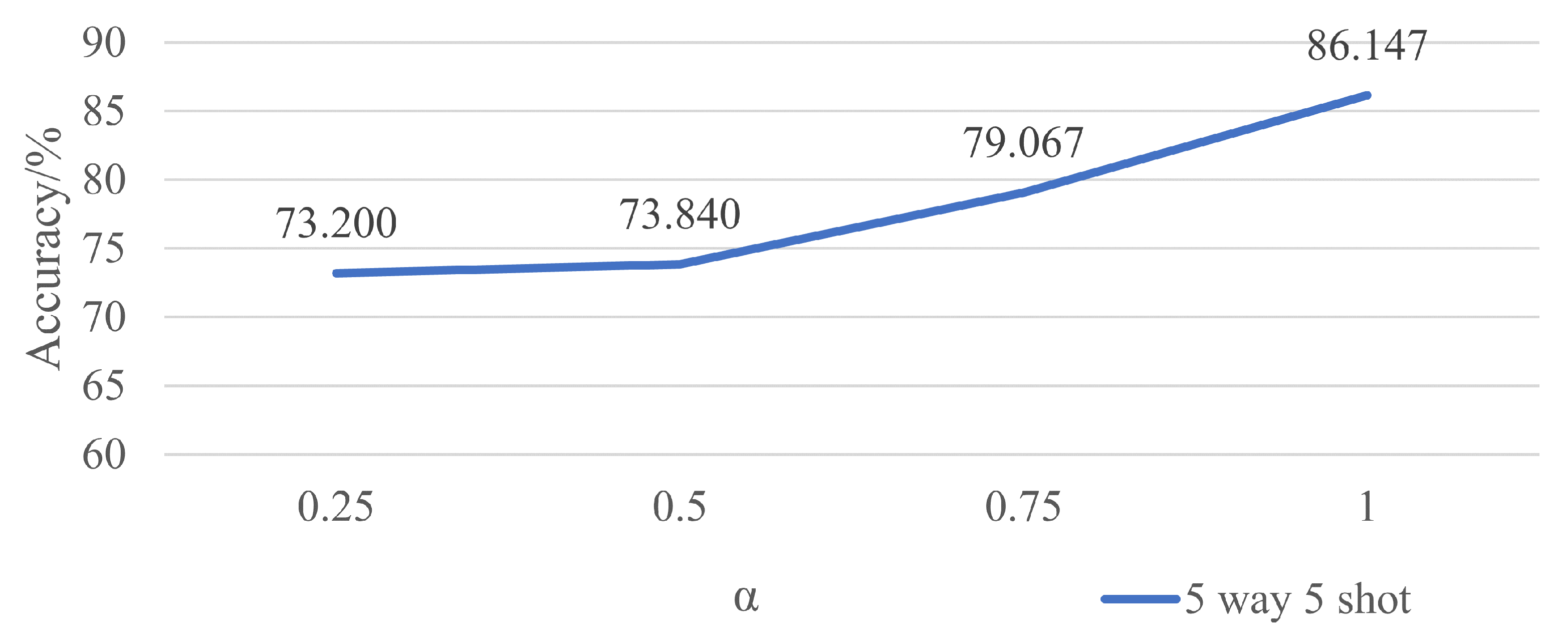
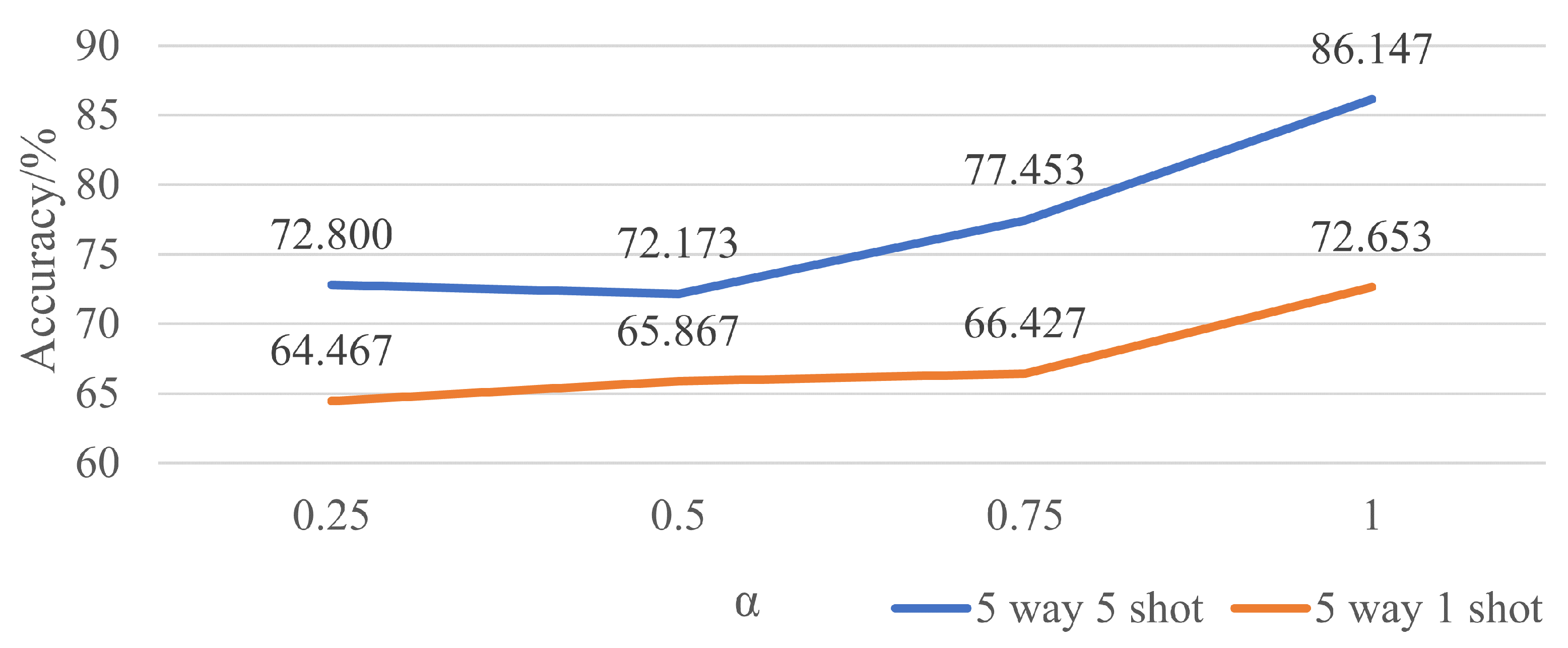
Furthermore, as we restrict the geometric transformations to rotations, there are further improvements in accuracy. That makes sense because all these images included are taken under the same circumstances with only a difference in azimuth. Each has the target right in the middle. Thus, translation does not work when it comes to accuracy. Shearing and scaling also cut no ice since they will narrow the gap between different classes as well as magnify that of the same class to some extent.

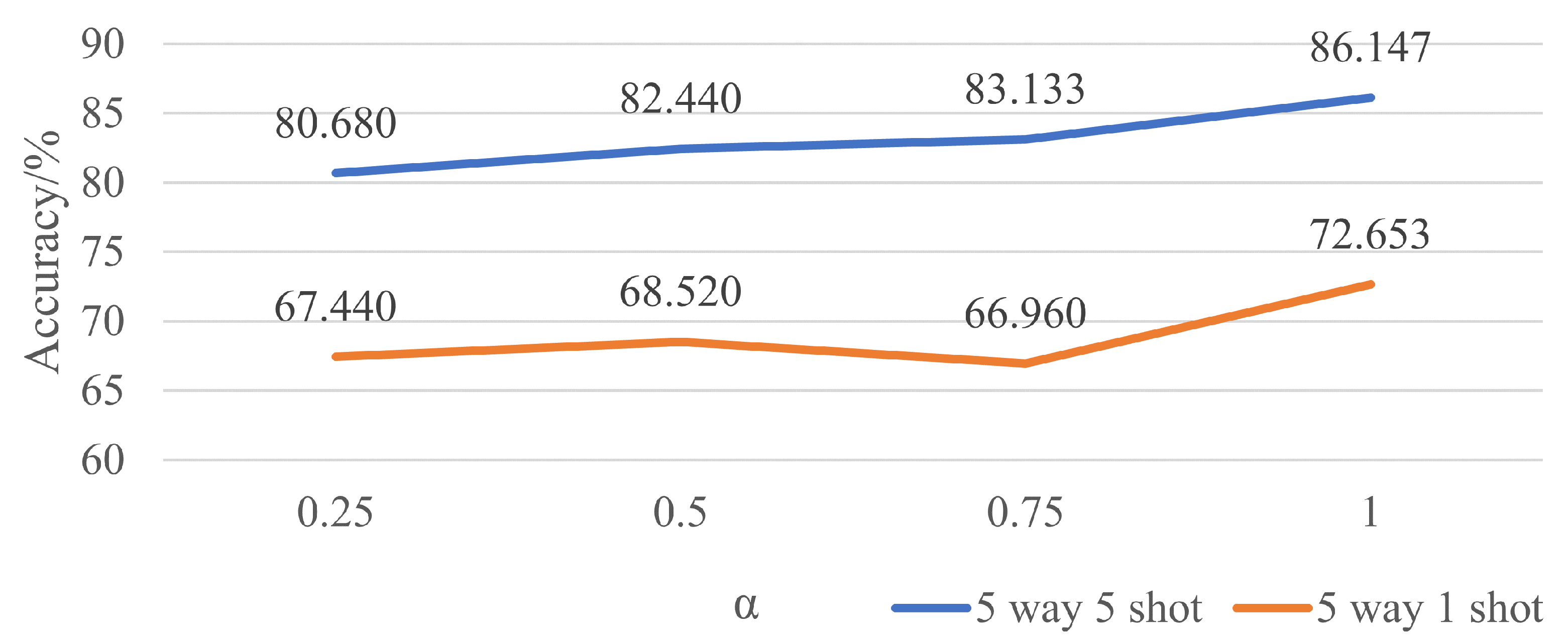
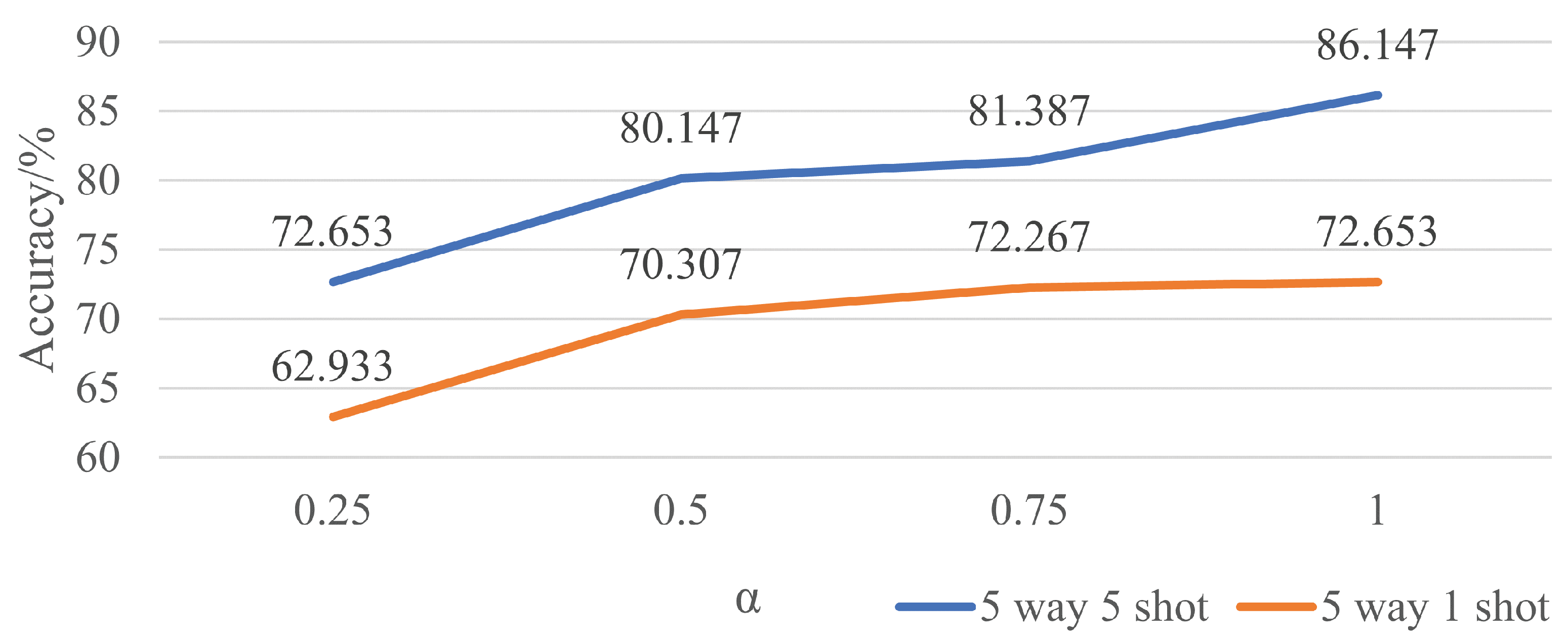
As the ablation study reveals that cos$\theta$ fits better than $\theta$, there is an improvement of 3.960% in 5-way 5-shot experiments and 9.386% in 5-way 1-shot experiments, respectively, which is literally a big step forward. What may cause this situation is that cos$\theta$ is a periodic function against $\theta$, and multiple $\theta$s can result in the same cos$\theta$, which may confuse the machine to fit the best parameters. That is why although there is a slight improvement when $\theta$ is applied in five-way five-shot experiments, there is a great loss in five-way one-shot experiments. Until now, a rotation transformation with cos$\theta$ as the regression parameter stands out with 86.147% for 5-way 5-shot experiments and 72.653% for 5-way 1-shot experiments.

Another ablation study shows that a single cross-entropy loss is the best loss function of all. Either with extra loss from an additional softmax layer or from clustering of support set or the whole set, the larger the proportion of original cross-entropy loss is, the better accuracy it will achieve. So it did with an extra contrastive loss. All four attempts try to restrict the distribution of the data to a better-organized one. However, they all work the opposite, which demonstrates that a single cross-entropy loss is already complex enough to fit the current dataset.

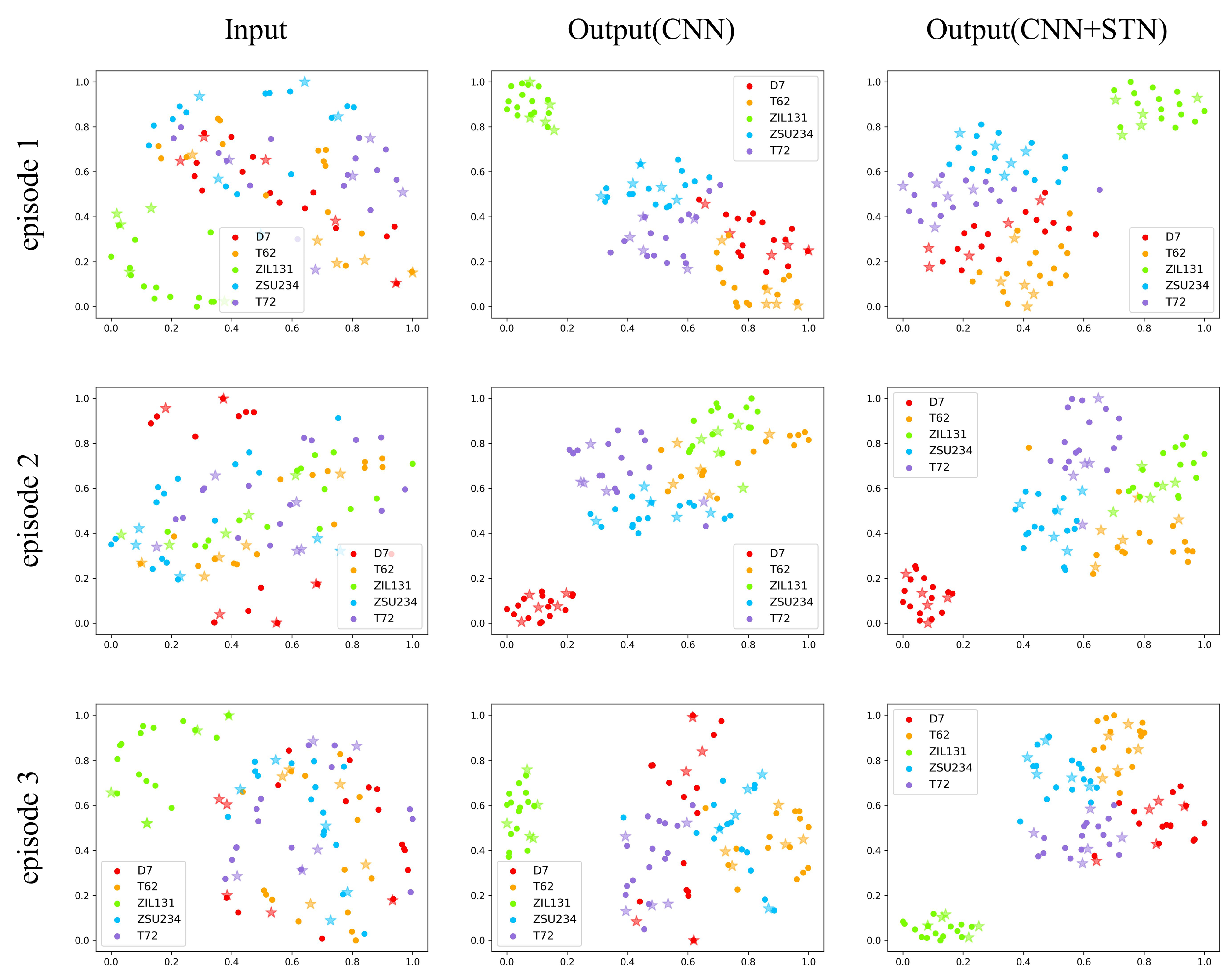
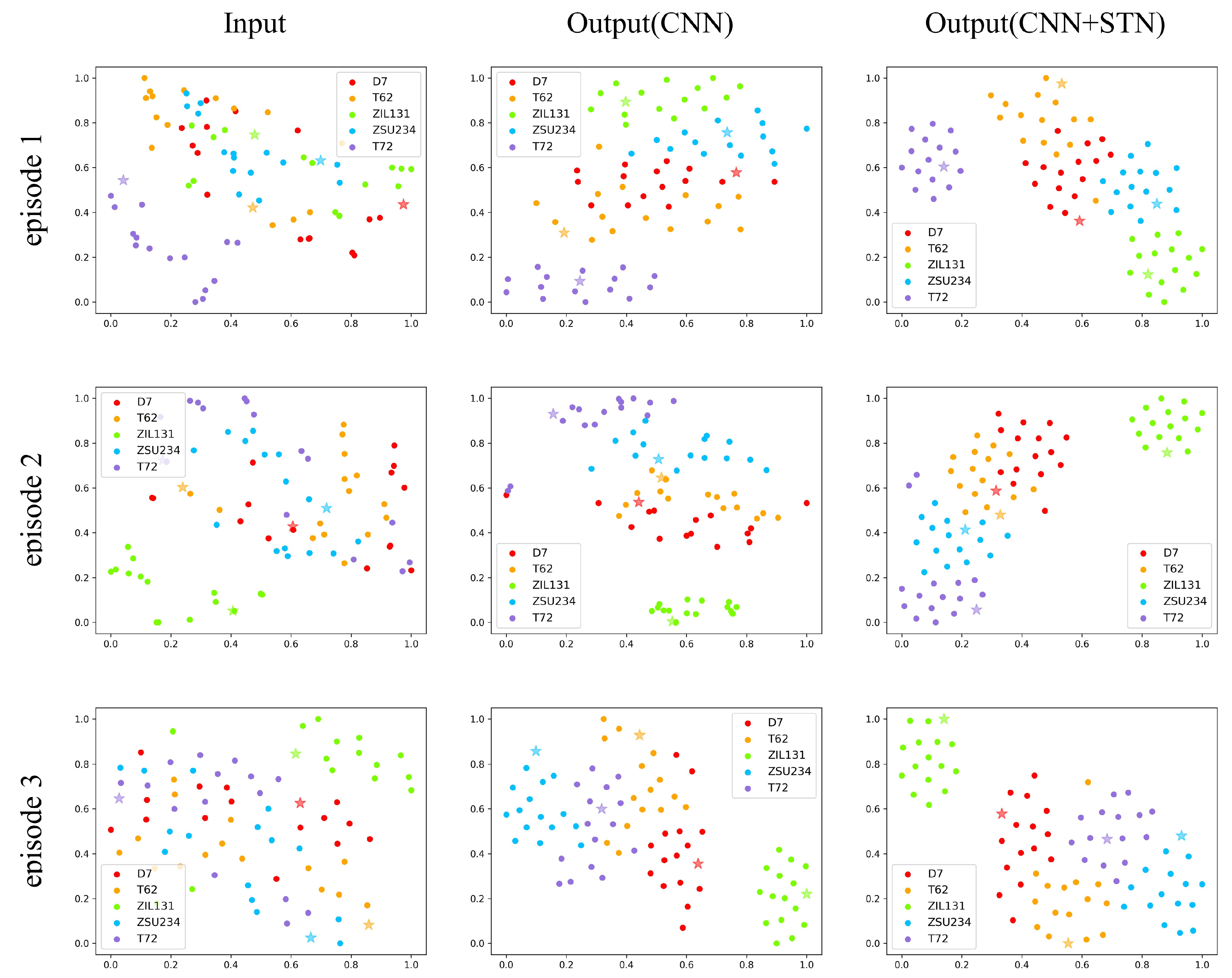
The visualization results of the three episodes show a random distribution at the beginning due to a vast difference in values of pixels, which is also consistent with the previous location experiments. After being extracted by a four-layer CNN, there is a better-organized situation allowing features of the same class to be closer to each other while separating features of variant classes. Still, it is relatively scattered out there. With a final spatial transformer module cascaded, a more centralized distribution exists, which is more obvious in five-way one-shot visualizations. That is because when rotation is conducted on these targets, the distance between features of the same class becomes even smaller. Clearly, it is another proof of the effectiveness of our algorithm.

While we have obtained an encouraging result, there are still some more things to do. Since we only experimented with four kinds of extra loss functions and simply added them together with weight to form an overall loss function, we recommend that there is another combination of loss functions. In addition, as we set the weight of two parts of loss to be added as 1, an accurate weight needs to be experimented with. What is more, as STM is cascaded after the last convolutional layer of each backbone, we believe that the relationship between the support set and query set is needed to be taken into consideration when regressing the transformation parameter $\mathsf{\Theta }$, which leads to future experiments.

6. Conclusions

In this study, we introduced a spatial transformer module to the original Prototypical Network, known as ST-PN. By cascading an STM after the last convolutional layer, some more latent information is exploited, and fewer parameters will be included. We restrict the transformation to rotation for the reason that azimuth causes the biggest difference among targets of the same class. What is more, cos$\theta$ is set to be the only parameter that needs to be regressed. While multiple $\theta$s may result in the same cos$\theta$, it is literally confusing for the machine to decide which data are the best ones. In addition, the experimental results of the four extra losses have already verified the effectiveness of a single cross-entropy loss. Among all other FSL methods, ST-PN achieves state-of-the-art performance for at least 5 percent of improvement. As revealed in the visualization results, there is a more organized as well as centralized distribution due to the application of spatial transformation.

References

1. Hong, D.; Gao, L.; Yokoya, N.; Yao, J.; Chanussot, J.; Du, Q.; Zhang, B. More diverse means better: Multimodal deep learning meets remote-sensing imagery classification. IEEE Trans. Geosci. Remote Sens. 2020, 59, 4340–4354. [Google Scholar] [CrossRef]
2. Alajaji, D.; Alhichri, H.S.; Ammour, N.; Alajlan, N. Few-shot learning for remote sensing scene classification. In Proceedings of the 2020 Mediterranean and Middle-East Geoscience and Remote Sensing Symposium (M2GARSS), Tunis, Tunisia, 9–11 March 2020; pp. 81–84. [Google Scholar]
3. Geng, J.; Deng, X.; Ma, X.; Jiang, W. Transfer learning for SAR image classification via deep joint distribution adaptation networks. IEEE Trans. Geosci. Remote Sens. 2020, 58, 5377–5392. [Google Scholar] [CrossRef]
4. Yang, R.; Xu, X.; Li, X.; Wang, L.; Pu, F. Learning Relation by Graph Neural Network for SAR Image Few-Shot Learning. In Proceedings of the IGARSS 2020-2020 IEEE International Geoscience and Remote Sensing Symposium, Waikoloa, HI, USA, 26 September–2 October 2020; pp. 1743–1746. [Google Scholar]
5. Wang, Y.; Yao, Q.; Kwok, J.T.; Ni, L.M. Generalizing from a few examples: A survey on few-shot learning. ACM Comput. Surv. (CSUR) 2020, 53, 1–34. [Google Scholar] [CrossRef]
6. Zhu, H.; Wang, W.; Leung, R. SAR target classification based on radar image luminance analysis by deep learning. IEEE Sens. Lett. 2020, 4, 7000804. [Google Scholar] [CrossRef]
7. Zhu, H.; Leung, R.; Hong, M. Shadow compensation for synthetic aperture radar target classification by dual parallel generative adversarial network. IEEE Sens. Lett. 2020, 4, 7002904. [Google Scholar] [CrossRef]
8. Ding, B.; Wen, G.; Huang, X.; Ma, C.; Yang, X. Target recognition in SAR images by exploiting the azimuth sensitivity. Remote Sens. Lett. 2017, 8, 821–830. [Google Scholar] [CrossRef]
9. Papson, S.; Narayanan, R.M. Classification via the shadow region in SAR imagery. IEEE Trans. Aerosp. Electron. Syst. 2012, 48, 969–980. [Google Scholar] [CrossRef]
10. Cui, J.; Gudnason, J.; Brookes, M. Radar shadow and superresolution features for automatic recognition of MSTAR targets. In Proceedings of the IEEE International Radar Conference, Arlington, VA, USA, 9–12 May 2005; pp. 534–539. [Google Scholar]
11. Furukawa, H. Deep learning for target classification from SAR imagery: Data augmentation and translation invariance. arXiv 2017, arXiv:1708.07920. [Google Scholar]
12. Lv, J.; Liu, Y. Data augmentation based on attributed scattering centers to train robust CNN for SAR ATR. IEEE Access 2019, 7, 25459–25473. [Google Scholar] [CrossRef]
13. Wang, C.; Shi, J.; Zhou, Y.; Yang, X.; Zhou, Z.; Wei, S.; Zhang, X. Semisupervised Learning-Based SAR ATR via Self-Consistent Augmentation. IEEE Trans. Geosci. Remote Sens. 2020, 59, 4862–4873. [Google Scholar] [CrossRef]
14. Miller, E.G.; Matsakis, N.E.; Viola, P.A. Learning from one example through shared densities on transforms. In Proceedings of the IEEE Conference on Computer Vision and Pattern Recognition CVPR 2000 (Cat. No. PR00662), Hilton Head Island, SC, USA, 15 June 2000; Volume 1, pp. 464–471. [Google Scholar]
15. Schwartz, E.; Karlinsky, L.; Shtok, J.; Harary, S.; Marder, M.; Kumar, A.; Feris, R.; Giryes, R.; Bronstein, A. Delta-encoder: An effective sample synthesis method for few-shot object recognition. arXiv 2018, arXiv:1806.04734. [Google Scholar]
16. Yan, Y.; Sun, J.; Yu, J. Prototype metric network for few-shot radar target recognition. In Proceedings of the IET International Radar Conference (IET IRC 2020), Chongqing, China, 4–6 November 2020; Volume 2020, pp. 1102–1107. [Google Scholar]
17. He, K.; Zhang, X.; Ren, S.; Sun, J. Deep residual learning for image recognition. In Proceedings of the IEEE Conference on Computer Vision and Pattern Recognition, Las Vegas, NV, USA, 27–30 June 2016; pp. 770–778. [Google Scholar]
18. Wang, C.; Gu, H.; Su, W. SAR Image Classification Using Contrastive Learning and Pseudo-Labels With Limited Data. IEEE Geosci. Remote Sens. Lett. 2021, 19, 4012505. [Google Scholar] [CrossRef]
19. Shang, R.; Wang, J.; Jiao, L.; Stolkin, R.; Hou, B.; Li, Y. SAR targets classification based on deep memory convolution neural networks and transfer parameters. IEEE J. Sel. Top. Appl. Earth Obs. Remote Sens. 2018, 11, 2834–2846. [Google Scholar] [CrossRef]
20. Geng, J.; Wang, H.; Fan, J.; Ma, X. SAR image classification via deep recurrent encoding neural networks. IEEE Trans. Geosci. Remote Sens. 2017, 56, 2255–2269. [Google Scholar] [CrossRef]
21. Rußwurm, M.; Wang, S.; Korner, M.; Lobell, D. Meta-learning for few-shot land cover classification. In Proceedings of the IEEE/CVF Conference on Computer Vision and Pattern Recognition Workshops, Seattle, WA, USA, 14–19 June 2020; pp. 200–201. [Google Scholar]
22. Fu, K.; Zhang, T.; Zhang, Y.; Wang, Z.; Sun, X. Few-Shot SAR Target Classification via Metalearning. IEEE Trans. Geosci. Remote Sens. 2021, 60, 2000314. [Google Scholar] [CrossRef]
23. Snell, J.; Swersky, K.; Zemel, R.S. Prototypical networks for few-shot learning. arXiv 2017, arXiv:1703.05175. [Google Scholar]
24. Ding, J.; Chen, B.; Liu, H.; Huang, M. Convolutional neural network with data augmentation for SAR target recognition. IEEE Geosci. Remote Sens. Lett. 2016, 13, 364–368. [Google Scholar] [CrossRef]
25. Chen, S.; Wang, H.; Xu, F.; Jin, Y.Q. Target classification using the deep convolutional networks for SAR images. IEEE Trans. Geosci. Remote Sens. 2016, 54, 4806–4817. [Google Scholar] [CrossRef]
26. Hou, R.; Chang, H.; Ma, B.; Shan, S.; Chen, X. Cross attention network for few-shot classification. arXiv 2019, arXiv:1910.07677. [Google Scholar]
27. Jaderberg, M.; Simonyan, K.; Zisserman, A. Spatial transformer networks. Adv. Neural Inf. Process. Syst. 2015, 28, 2017–2025. [Google Scholar]
28. Vanschoren, J. Meta-learning: A survey. arXiv 2018, arXiv:1810.03548. [Google Scholar]
29. Finn, C.; Abbeel, P.; Levine, S. Model-agnostic meta-learning for fast adaptation of deep networks. In Proceedings of the International Conference on Machine Learning, Sydney, Australia, 6–11 August 2017; pp. 1126–1135. [Google Scholar]
30. Nichol, A.; Schulman, J. Reptile: A scalable metalearning algorithm. arXiv 2018, arXiv:1803.02999. [Google Scholar]
31. Ye, H.J.; Hu, H.; Zhan, D.C.; Sha, F. Few-shot learning via embedding adaptation with set-to-set functions. In Proceedings of the IEEE/CVF Conference on Computer Vision and Pattern Recognition, Seattle, WA, USA, 13–19 June 2020; pp. 8808–8817. [Google Scholar]
32. Kaiser, Ł.; Nachum, O.; Roy, A.; Bengio, S. Learning to remember rare events. arXiv 2017, arXiv:1703.03129. [Google Scholar]
33. Chopra, S.; Hadsell, R.; LeCun, Y. Learning a similarity metric discriminatively, with application to face verification. In Proceedings of the 2005 IEEE Computer Society Conference on Computer Vision and Pattern Recognition (CVPR’05), San Diego, CA, USA, 20–25 June 2005; Volume 1, pp. 539–546. [Google Scholar]
34. Vinyals, O.; Blundell, C.; Lillicrap, T.; Wierstra, D. Matching networks for one shot learning. Adv. Neural Inf. Process. Syst. 2016, 29, 3630–3638. [Google Scholar]
35. Sung, F.; Yang, Y.; Zhang, L.; Xiang, T.; Torr, P.H.; Hospedales, T.M. Learning to compare: Relation network for few-shot learning. In Proceedings of the IEEE Conference on Computer Vision and Pattern Recognition, Salt Lake City, UT, USA, 18–22 June 2018; pp. 1199–1208. [Google Scholar]
36. Gao, K.; Liu, B.; Yu, X.; Qin, J.; Zhang, P.; Tan, X. Deep relation network for hyperspectral image few-shot classification. Remote Sens. 2020, 12, 923. [Google Scholar] [CrossRef] [Green Version]
37. Garcia, V.; Bruna, J. Few-shot learning with graph neural networks. arXiv 2017, arXiv:1711.04043. [Google Scholar]
38. Wang, L.; Bai, X.; Zhou, F. Few-Shot SAR ATR Based on Conv-BiLSTM Prototypical Networks. In Proceedings of the 2019 6th Asia-Pacific Conference on Synthetic Aperture Radar (APSAR), Xiamen, China, 26–29 November 2019; pp. 1–5. [Google Scholar]
39. Tang, J.; Zhang, F.; Zhou, Y.; Yin, Q.; Hu, W. A fast inference networks for SAR target few-shot learning based on improved siamese networks. In Proceedings of the IGARSS 2019–2019 IEEE International Geoscience and Remote Sensing Symposium, Yokohama, Japan, 28 July–2 August 2019; pp. 1212–1215. [Google Scholar]
40. Lu, D.; Cao, L.; Liu, H. Few-Shot Learning Neural Network for SAR Target Recognition. In Proceedings of the 2019 6th Asia-Pacific Conference on Synthetic Aperture Radar (APSAR), Xiamen, China, 26–29 November 2019; pp. 1–4. [Google Scholar]
41. Rostami, M.; Kolouri, S.; Eaton, E.; Kim, K. Sar image classification using few-shot cross-domain transfer learning. In Proceedings of the IEEE/CVF Conference on Computer Vision and Pattern Recognition Workshops, Beach, CA, USA, 16–17 June 2019. [Google Scholar]
42. Wang, L.; Bai, X.; Gong, C.; Zhou, F. Hybrid Inference Network for Few-Shot SAR Automatic Target Recognition. IEEE Trans. Geosci. Remote Sens. 2021, 59, 9257–9269. [Google Scholar] [CrossRef]
43. Li, W.; Dong, C.; Tian, P.; Qin, T.; Yang, X.; Wang, Z.; Huo, J.; Shi, Y.; Wang, L.; Gao, Y.; et al. LibFewShot: A Comprehensive Library for Few-shot Learning. arXiv 2021, arXiv:2109.04898. [Google Scholar]
Figure 1. A demonstration of FSL.
Remotesensing 14 02019 g001
Figure 2. Overall architecture of the proposed Prototypical Network based on Spatial Transformation (ST-PN). The embedding module extracts and aligns features from input images, which is shown in detail in the lower part of the figure. Euclidean distance is calculated between a query sample and each class prototype to represent their similarity.
Remotesensing 14 02019 g002
Figure 3. Three kinds of affine transformation.
Remotesensing 14 02019 g003
Figure 4. The architecture of CNN as the backbone.
Remotesensing 14 02019 g004
Figure 5. Optical and SAR images of 10 vehicles in MSTAR dataset.
Remotesensing 14 02019 g005
Figure 6. T-SNE visualization results of the whole stages of three individual episodes for five-way dive-shot experiments. Each column denotes a stage and each row denotes an episode. Images in the left column indicate the visualization results of the input, outputs of CNN in the middle, and outputs of STN cascaded after CNN in the right. Note that each solid circle and star of the same color stands for the same class.
Remotesensing 14 02019 g006
Figure 7. T-SNE visualization results of the whole stages of three individual episodes for five-way one-shot experiments. Each column denotes a stage and each row denotes an episode. Images in the left column indicate visualization results of input, outputs of CNN in the middle, and outputs of STN cascaded after CNN on the right. Note that each solid circle and star of the same color stands for the same class.
Remotesensing 14 02019 g007
Figure 8. Experiments on extra loss from additional softmax layer against α in both five-way one-shot and five-way five-shot settings.
Remotesensing 14 02019 g008
Figure 9. Experiments on extra loss from clustering of support set against α in a five-way five-shot setting.
Remotesensing 14 02019 g009
Figure 10. Experiments on extra loss from clustering of the whole set against α in both five-way one-shot and five-way five-shot settings.
Remotesensing 14 02019 g010
Figure 11. Experiments on extra loss from contrastive loss against α in both five-way one-shot and five-way five-shot settings.
Remotesensing 14 02019 g011