Field Data Collection Methods Strongly Affect Satellite-Based Crop Yield Estimation

Abstract

Crop yield estimation from satellite data requires field observations to fit and evaluate predictive models. However, it is not clear how much field data collection methods matter for predictive performance. To evaluate this, we used maize yield estimates obtained with seven field methods (two farmer estimates, two point transects, and three crop cut methods) and the “true yield” measured from a full-field harvest for 196 fields in three districts in Ethiopia in 2019. We used a combination of nine vegetation indices and five temporal aggregation methods for the growing season from Sentinel-2 SR data as yield predictors in the linear regression and Random Forest models. Crop-cut-based models had the highest model fit and accuracy, similar to that of full-field-harvest-based models. When the farmer estimates were used as the training data, the prediction gain was negligible, indicating very little advantage to using remote sensing to predict yield when the training data quality is low. Our results suggest that remote sensing models to estimate crop yield should be fit with data from crop cuts or comparable high-quality measurements, which give better prediction results than low-quality training data sets, even when much larger numbers of such observations are available.

1. Introduction

The lack of accurate, high-spatial-resolution crop yield data constrains research, policy, and business development. Accurate yield data are needed for crop insurance [1,2], farm advisory services, understanding how productivity responds to environmental change [3], forecasting commodity prices [4], and assessing opportunities for increasing production [5]. In the absence of reliable data reported by producers or government agencies, crop yield can be estimated with remotely sensed data [6,7].

Remote-sensing-based yield prediction models are typically constructed with field observations of crop yield and corresponding reflectance data from satellite-based sensors. There has been ample research comparing modeling methods [7,8,9,10,11], but not much attention has been given to the effect of the field data collection method and sample size on model quality. This is important to consider because measuring crop yield in the field is generally expensive, and the costs may differ considerably between methods. Modern agricultural harvesting machinery can monitor the mass flow of crops in real time [12,13]; however, this technology is not available in many areas. A relatively straightforward method is to ask farmers what their yield was or what it will be. This may be the only available approach after crops have been harvested or when it is still too early to harvest, and it has been used to understand longer-term annual variability in crop yields [2]. Such approaches may provide accurate yield estimates under certain conditions, especially if all produce is weighed and sold to a single source. In developing countries, this is often not the case, and farmer estimates are likely to be inaccurate [14]; using such data may lead to poor predictive models [15]. An additional problem is a potential bias in farmers’ estimates if they perceive that their responses may influence subsequent taxation or benefit allocations [15,16].

As an alternative to farmer reports, crop yield can be estimated based on a variety of field sampling techniques. The crop cut method is often considered the best sampling method to estimate crop yield [17]. In this method, one or a few small areas within a field are harvested and weighed. However, crop cuts can lead to yield overestimation because areas within the field with poor crop stands are more likely to be under-sampled [18]. This may be addressed by randomly selecting (multiple) crop cut locations within a field. Alternatively, point transect methods can be used to sample a fixed number of plants and to estimate plant density at random or systematic intervals, thus allowing for an estimation of crop yield with generally lower costs of data collection [19,20].

As there are different field estimation methods available, selecting the best method requires balancing the costs (time, money) and benefits (accuracy in estimating crop yield). While it is generally better to have data from more fields and larger samples within fields, it is not clear whether it would be preferable to make noisy observations of many fields or highly accurate (and more expensive) observations of fewer fields. Given a fixed level of available resources (time or money), models built with a larger data set of lower-quality data could outperform models built with a small quantity of high-quality data. Understanding these tradeoffs may provide important practical guidance for optimizing training data collection efforts.

To address this question, we evaluated the effect of field estimation methods on crop yield prediction, using a dataset for 196 maize fields in Ethiopia for which yield was estimated with seven different sampling methods. Maize is the dominant food crop in much of East Africa, and estimating maize yield for satellite data is an active area of research [21]. We used linear regression and Random Forest models to estimate crop yield in response to vegetation indices derived from Sentinel-2 reflectance data. Model accuracy is typically evaluated with cross-validation and the implicit assumption that the field observations are without error. In our study, we evaluated the models’ internal accuracy with standard cross-validation and their external accuracy by evaluating them with the true yield data obtained by harvesting entire fields.

2. Materials and Methods

2.1. Field Data Collection

Maize yield data were collected in 2019 in three woredas (districts) in Ethiopia’s Amhara Region: Dera, Fenote Selam, and Merawi. In each woreda, the survey team coordinated with extension services to identify maize farmers willing to harvest their fields in collaboration with the survey team. Samples were taken from 7–29 November 2019, coinciding with the maize harvest season in these areas. Prior to field data collection, farmers were asked to estimate the size and maize production of their fields. One group of enumerators walked field boundaries with GPS receivers. Another group took yield measurements using the sampling protocols described below and used GPS receivers to locate the subplots used in the crop cuts. All field boundaries and crop cut locations were visually checked by plotting them on high-resolution satellite images for the same season, and minor errors were corrected where necessary. The resulting dataset contained information on 227 fields. We discarded the data for 3 fields because of inconsistent coordinates, and 28 fields were so small that they did not contain a single 20 m pixel from Sentinel-2. The resulting 196 fields consisted of 52 fields in Dera, 67 in Fenote Selam, and 77 in Merawi. Field sizes ranged from 0.06 to 0.29 ha (median = 0.13 ha; mean = 0.14 ha) or between 4 and 30 pixels (median = 14, mean = 15.16).

Seven sampling methods were used to estimate maize grain yield (kg/ha) for each field (

Table 1. Field sampling methods used to estimate and measure maize yield in fields in Ethiopia and relative time, i.e., the amount of time spent in the field to estimate yield, relative to the “farmer yield” method.

Group	Name	Description	Relative Time
Farmer	Farmer yield	The farmer was asked for his/her estimate of production in quintals (1 quintal is 100 kg) and of the area of his/her field.	1
	Farmer production	The farmer was asked for his/her estimate of production in quintals, and enumerators measured the field area.	1.5
Transect	Edge transect	Enumerators walked along the two opposite long sides of the field, taking samples at five equally spaced points at each side (1 m from the field edge). At each point, three cobs were harvested. Yield was computed by multiplying average cob yield with estimated cob density. To estimate cob density, at each sampling locus, the enumerators randomly selected three cobs and recorded the number of cob-bearing plants within 1 m${}^2$ of the area surrounding the sampling points.	3.5
	Mid-transect	Enumerators walked along the line that connects the mid-points of the short sides of the field, taking samples at four equally spaces points. At each point, three cobs were harvested. Yield was computed by multiplying average cob yield with estimated cob density.	2.2
Cut	Random cut	Enumerators determined a single sub-plot location using a random distance along two sides of the field, 1 m from the field edge. The sub-plot was 4 × 4 m, and yield was measured by harvesting all plants within.	3.5
	Center cut	As above, but the sub-plot was located at the center of the field.	3.5
	Diagonal cuts	As above, but for three sub-plots, located at equal distances along the longest field diagonal, including the center crop cut.	4.4
Field	Full field	The entire field was harvested to determine the true yield	35.6

). For methods that involved harvesting a sample, cobs were left after weighing where the plant was located to avoid counting errors when one sampling method overlapped with another. After these sampling methods were completed, the entire field was harvested. Subsamples of the grain were taken for each field to determine moisture content. This was used to standardize all the yield data to 12.5% moisture.

2.2. Satellite Data

We used Sentinel-2 surface reflectance (SR) data for the growing season (July–November 2019). Collectively, the European Space Agency (ESA) twin satellites, Sentinel-2A and Sentinel-2B, referred to as Sentinel-2, have 13 spectral bands from visible to shortwave infrared at 10–20 m resolution and a five-day revisit period. Sentinel-2 SR has been processed with an atmospheric correction applied to top-of-atmosphere (TOA) Level-1C orthoimage products. In addition, we used a cloud mask to remove cloudy pixels. We used Google Earth Engine to download data for all pixels in each field using a 5 m negative buffer to ensure that pixels were entirely within fields and to account for some imprecision in field boundaries.

Reflectance data used for yield prediction are commonly transformed into vegetation indices (VIs) for the growing season [11,22]. VIs used for this purpose include NDVI [23,24,25], red-edge VIs [24,26,27,28,29], and GCVI [9,30]. We computed and used nine different indices (

Table 2. Vegetation indices (VIs) used, their abbreviation (Abbr.), and the equation used to compute them with Sentinel-2 bands: Blue (band 2) = 494 nm, Green (band 3) = 560 nm, red (band 4) = 665, Red edge (band 5) = 704 nm, Red edge 2 (band 6) = 740 nm, Red_edge_3 (band 7) = 780 nm, NIR (band 8) = 834 nm, Red edge 4 (band 8A) = 864 nm, SWIR 1 (band 11) = 1612 nm, SWIR2 (band 12) = 2194 nm.

Vegetation Index (VI)	Abbr.	Equation
Chlorophyll Red edge	ChlRE	(Red_edge_1/Red_edge_3)
Enhanced VI	EVI	2.5 × (NIR − Red)/((NIR + 6 × Red − 7.5 × Blue) + 1)
Green-brown VI	GBVI	(Blue − Green)/(Blue + Green)
Green chlorophyll VI	GCVI	(NIR/Green) − 1
Green-red VI	GRVI	(Green − Red)/(Green + Red)
Green normalized difference VI	GNDVI	(NIR − Green)/(NIR + Green)
Modified anthocyanin reflectance index	mARI	(1/Green) − (1/Red_edge_1)) × Red_edge_3
Moisture stress index	MSI	SWIR1/NIR
Normalized difference VI	NDVI	(NIR − Red)/(NIR + Red)

).

2.3. Growing Season Aggregates

We used composites of VIs for the growing season. We determined the timing of the growing season based on the green-up and senescence of each field or when NDVI values exceeded a threshold of 0.2, using the R package “phenex” [31]. We removed very low or high values (outliers) that were missed by the cloud filter, and we estimated missing values with interpolation and smoothed the VIs with the filterVI method from R package “luna” [32]. We then computed the median VI for all pixels of each field for each date to make the statistic less sensitive to outliers (in space or in time). We temporally aggregated the VI values for the growing season, for each field, with the following functions: sum, median, maximum, difference (max–min), and standard deviation. The seasonal sum or cumulative VI is a commonly used metric, as the accumulation of biomass, and hence crop yield, is assumed to be proportional to the cumulative greenness (NDVI) [22].

2.4. Modeling Methods and Evaluation

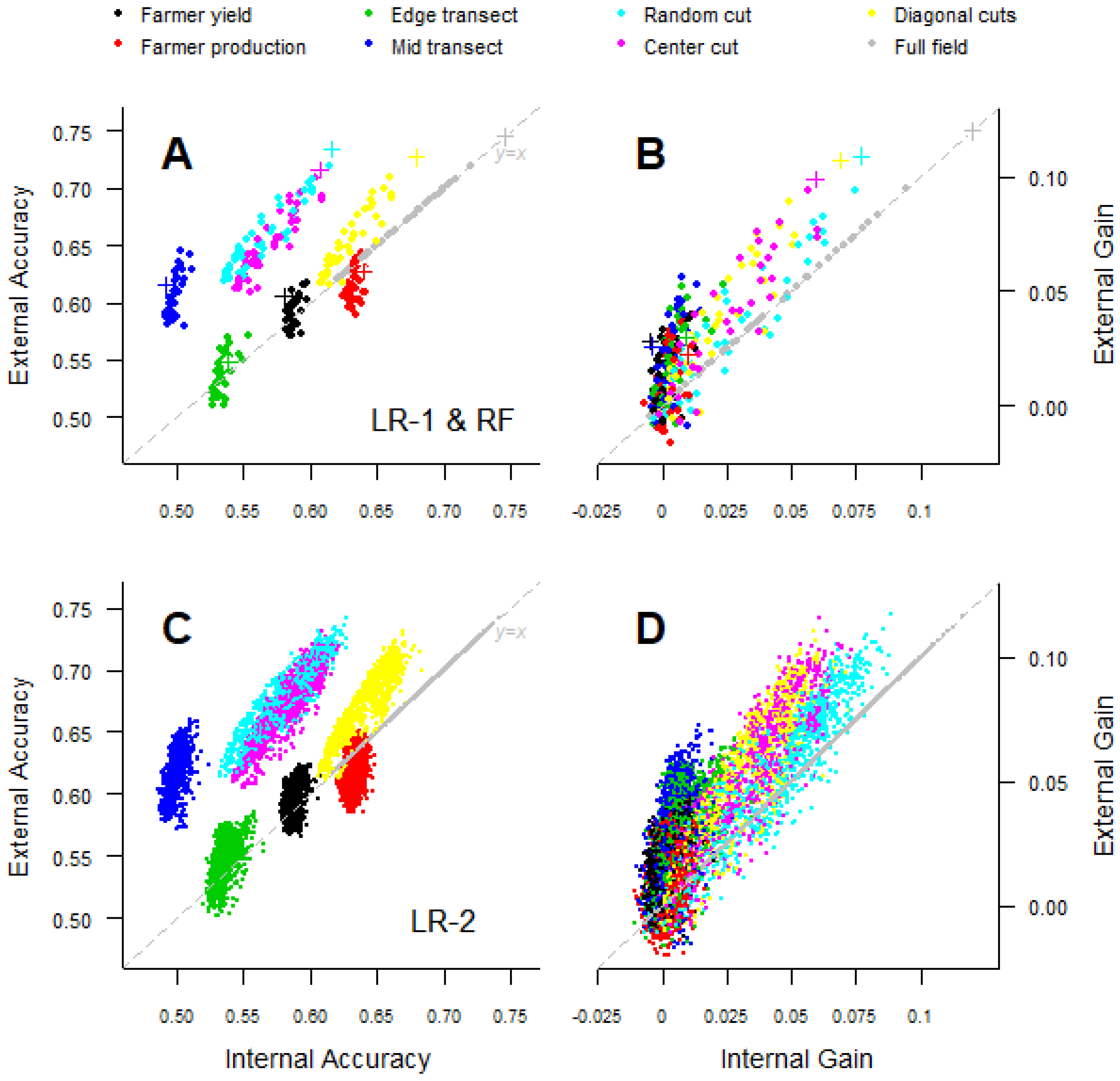
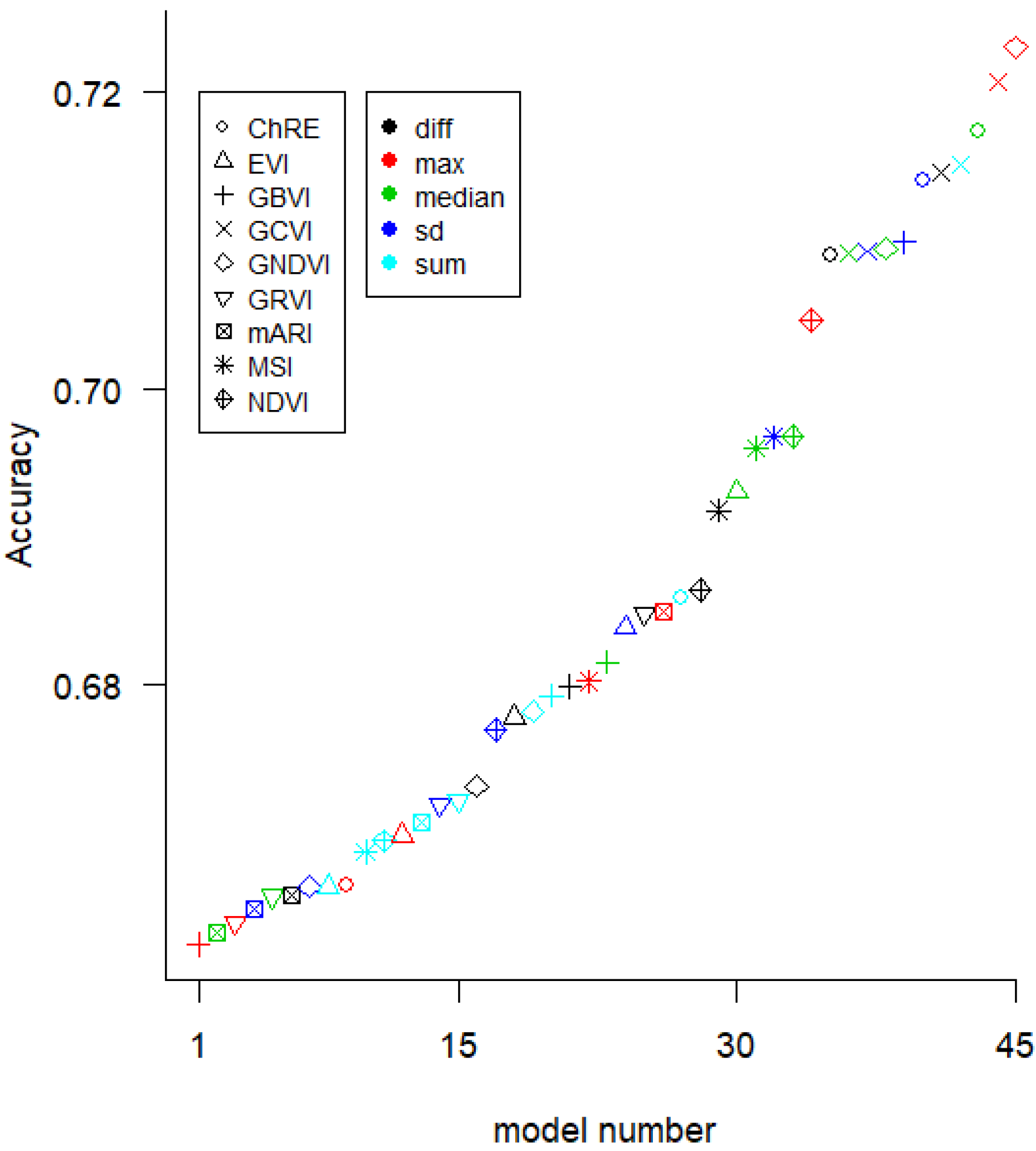
We used three modeling methods for the yield prediction models. First, we created 360 univariate ordinary least-squares (OLS) linear models (which we refer to as “LR-1”), one for each yield measurement, VI, and aggregation method (8 yield measurement methods × 9 VIs × 5 aggregation methods). Second, we created a Random Forest (RF) model using the 15 VI-(aggregation method) variables that performed best in the univariate linear models. Third, we made OLS regression models with two predictor variables (referred to as linear regression-2 “LR-2” in the text) for all 990 pairs of the 45 VI variables (9 VIs × 5 aggregation methods).

Models were evaluated with five-fold cross-validation. We assessed model fit with the proportion of explained variance ($R^2$) as the square of the Pearson correlation coefficient between observed and predicted values. We computed model accuracy (A) (Equation (1)) as one minus the root-mean-squared error (RMSE) standardized by the mean yield.

$$A_{efm}=1-\frac{\sqrt{\frac{{\sum }_{i=0}^n{({\hat{y}}_{ifm}-y_e)}^2}{n}}}{{\overline{y}}_e}$$

(1)

where y is crop yield for observation (field) i, field sampling method f, modeling method m, and number of observations n. $\overline{y}$ is the mean observed crop yield and $\hat{y}$ the predicted crop yield. Subscript e indicates the data used for the evaluation and can have these values: internal (INT), external (EXT), and extrapolation (TRA); see below. Thus, ${\hat{y}}_{ifm}$ refers to the predicted yield of field i using sampling method f and modeling method m and $y_e$ observed crop yield for a given evaluation method e. $A_{efm}$ refers either to $A_{INT}$, $A_{EXT}$, or $A_{TRA}$.

$A_{INT}$ (internal accuracy) is the standard RMSE. A weakness of this standard measure is that the observed data may be biased, and a high $A_{INT}$ could reflect that the model reproduces this bias. $A_{EXT}$ (external accuracy) evaluates the model with the “true yield”, as measured from the harvest of the entire field. This measure allows us to distinguish between a model that fits bad data well (high $A_{INT}$, but low $A_{EXT}$) from a model that predicts well (high $A_{EXT}$ and likely a high $A_{INT}$ as well). Furthermore, we evaluated the ability of models to extrapolate to other areas by using evaluation data from the regions other than the data used to fit the model ($A_{TRA}$). To calculate $A_{TRA}$, we used the fields from two woredas as the training data for the model and evaluated the model accuracy when predicting on the remaining woreda, for example using samples from the Dera and Fenote Selam woredas to predict the yield in Merawi.

We also computed a NULL model N (Equation (2)), which expresses the accuracy of using the mean value of all observations (either internal, external, or extrapolation) to predict the yield.

$$N_{ef}=1-\frac{\sqrt{\frac{{\sum }_{i=0}^n{({\hat{y}}_{if}-{\overline{y}}_e)}^2}{n}}}{{\overline{y}}_e}$$

(2)

We used the NULL model to compute the model gain G (Equation (3)), which is the model accuracy A minus the accuracy of the NULL model N

$$G_{efm}=A_{efm}-N_{ef}$$

(3)

As such, $G_{INT}$ gives the change in model accuracy compared to using the mean value, $G_{EXT}$ gives the change in model accuracy compared to the mean true yield, and $G_{TRA}$ gives the improvement to the models’ ability to extrapolate across regions compared to the mean true yield in the regions predicted.

2.5. Sample Size and Model Quality

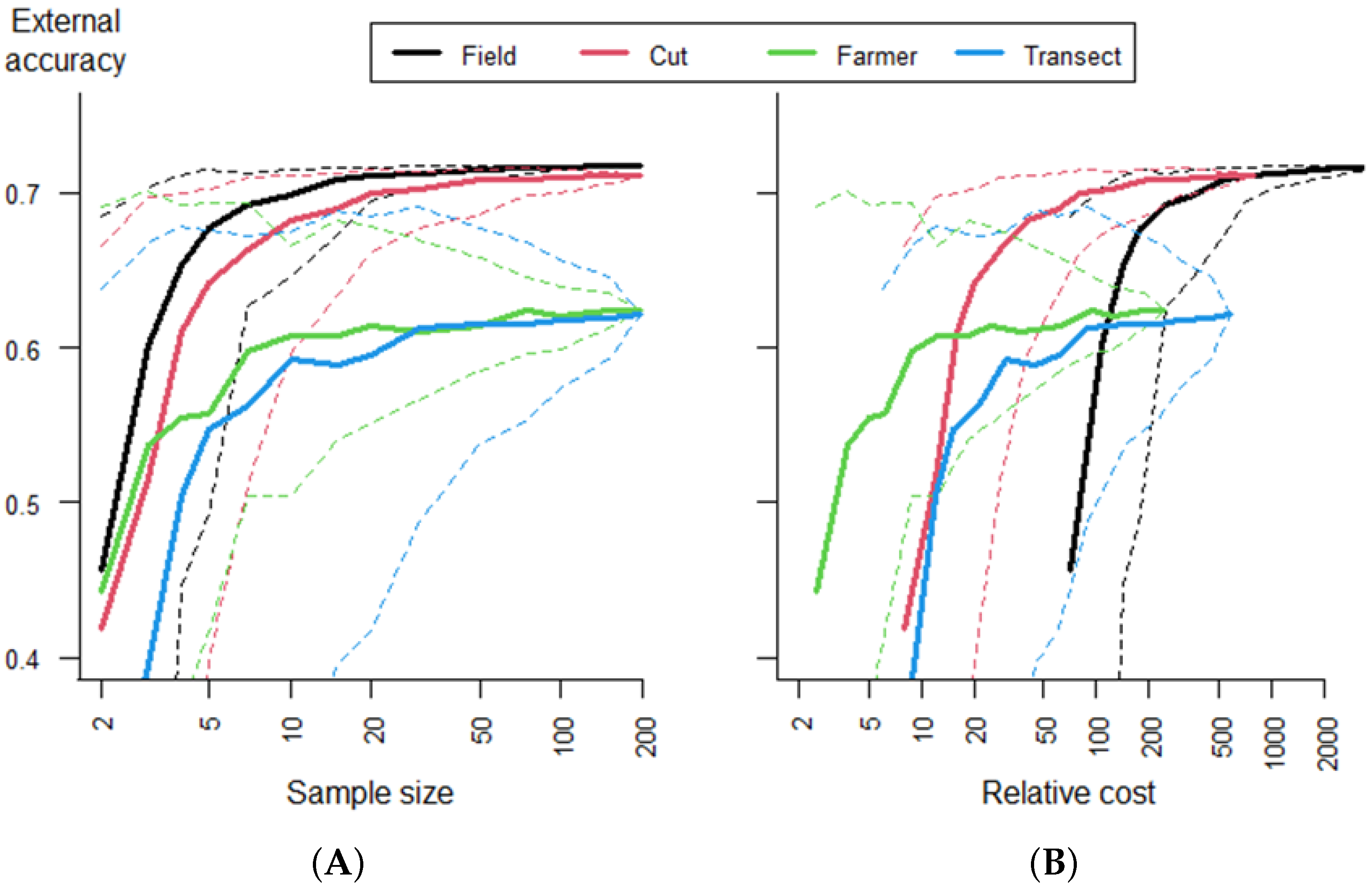
We estimated the cost per sample for each field method based on the time expense in the field for each method (Table 1). We assessed the tradeoff between the sample size (cost) and model accuracy using Monte Carlo simulation. For each field method, we drew 200 samples from the entire data set for each of the following sample sizes: 2, 3, 4, 5, 7, 10, 15, 20, 30, 50, 75, 100, 150, and 196, where each sample is one field. For each draw, all regression models were fit and evaluated. In the results, the “group” of each method was used in addition to the 8 methods. Groups include field (full field), cut (random cut, center cut, and three cuts), farmer (farmer yield and farmer production), and transect (mid- and edge transect).

3. Results

3.1. Field-Based Yield Estimates

The range of full-field harvest maize yields was between 898 and 11,158 kg/ha, with 80% between 4261 and 7338 kg/ha and a median of 6021 kg/ha. The association between the maize yield estimated from a sample and the true yield, as measured by the full-field harvest, strongly depended on the measurement method. Linear regression models of the yield estimated as a function of the true yield had an $R^2$ between 0.03 and 0.59 (Figure 1). The diagonal cuts method had the highest $R^2$ (0.59) and a slope of 0.84. The other two crop-cut methods had a slope that was closer to one (0.87), but a slightly lower model fit: the random cut $R^2$ was 0.47, while the center cut $R^2$ was 0.43. The model fit for transect estimates were much lower ($R^2$ = 0.2, with slopes of 0.7–0.75). There was hardly any association between the farmer estimates and the true yield. $R^2$ was 0.05 for the farmer yield (slope = 0.21) and 0.03 for the farmer production (slope = 0.18). Farmer estimates tended to be biased towards lower yields, while the transect methods were biased towards higher yields (Figure 1).

3.2. Internal and External Accuracy

The best models of maize yield as a function of one or more vegetation indices were more influenced by the field data than by the modeling method (

Table 3. Proportion of variation explained ($R^2$) for yield prediction models. The highest score for any of the 45 single-variable linear regression models (LR-1) or for the 990 two-variable linear regression models (LR-2) and for Random Forest (RF) models.

Field Method	LR-1	LR-2	RF
Farmer yield	0.10	0.14	0.06
Farmer production	0.11	0.14	0.09
Edge transect	0.11	0.16	0.08
Mid-transect	0.07	0.13	0.07
Random cut	0.31	0.35	0.35
Center cut	0.26	0.30	0.29
Diagonal cuts	0.26	0.35	0.32
Full field	0.44	0.52	0.52

). In all cases, the model with the full-field data had the highest $R^2$, followed by the models fit with crop cut data. The linear model with two variables (LR-2) had the highest $R^2$ values for the different sampling methods, and the Random Forest (RF) performed similarly for the full-field data. The single-variable regression models (LR-1) performed better than Random Forest for the farmer and transect yield estimates (Table 3).

The internal accuracy ($A_{INT}$) for the best predictor variables was between 0.72 and 0.75 for the three modeling methods when using the full-field data and ranged from 0.61 to 0.68 for the different crop cut samples. $A_{INT}$ was higher for the farmer estimates than for the transect data, and it was particularly low for the mid-transect (

Table 4. Internal ($A_{INT}$) and external accuracy ($A_{EXT}$) and gain ($G_{INT}$ and $G_{EXT}$) for models predicting maize yield from reflectance based on data from different field methods. Internal measures are based on standard cross-validation using data from a possibly inaccurate sample, whereas external measures compare predictions with true yield values. Accuracy is 1 for a perfect model and lower for other models. Gain is zero if the model is not better than the NULL model of observed mean yield. For each field method, we show the highest score for any of the 45 single-variable linear regression models (LR-1) or for the 990 two-variable linear regression models (LR-2) and for the Random Forest (RF) model.

	${\mathit{A}}_{\mathit{INT}}$			${\mathit{A}}_{\mathit{EXT}}$			${\mathit{G}}_{\mathit{INT}}$			${\mathit{G}}_{\mathit{EXT}}$
Field Method	LR-1	LR-2	RF	LR-1	LR-2	RF	LR-1	LR-2	RF	LR-1	LR-2	RF
Farmer yield	0.60	0.61	0.58	0.62	0.62	0.61	0.01	0.02	-0.01	0.04	0.05	0.03
Farmer prod.	0.64	0.65	0.64	0.64	0.65	0.63	0.01	0.02	0.01	0.04	0.05	0.02
Edge transect	0.55	0.56	0.54	0.57	0.59	0.55	0.02	0.03	0.01	0.05	0.07	0.03
Mid-transect	0.51	0.52	0.49	0.64	0.66	0.62	0.01	0.03	0.00	0.06	0.07	0.03
Random cut	0.61	0.63	0.62	0.72	0.74	0.73	0.07	0.09	0.08	0.09	0.12	0.11
Center cut	0.61	0.62	0.61	0.71	0.73	0.72	0.06	0.07	0.06	0.09	0.12	0.10
Diagonal cuts	0.66	0.68	0.68	0.71	0.73	0.73	0.05	0.07	0.07	0.09	0.11	0.11
Full field	0.72	0.74	0.75	0.72	0.74	0.75	0.09	0.12	0.12	0.09	0.12	0.12

, Figure 2).

For the crop cut data, the external accuracy ($A_{EXT}$) was higher than the internal accuracy ($A_{INT}$), and it was very similar for the different modeling methods (between 0.71 and 0.74) and hardly different from the accuracy for the full-field data (by definition, $A_{INT}$ and $A_{EXT}$ are the same for the full-field data). $A_{EXT}$ was very similar to $A_{INT}$ for the farmer estimates, but $A_{EXT}$ was higher for the mid-transect method, which performed as good as or better than the other non-crop cut measures, whereas the edge transect performed very poorly by this measure (Table 4, Figure 2).

For all modeling methods, the choice of VIs was very important when considering external accuracy and gain. VI selection caused a large amount of variability within each sampling method (Figure 2, Figure A1 and Figure A2). However, this sensitivity to the choice of predictor variables was much less when considering the internal measures for farmer estimates and transects (contrast the variation in the horizontal and vertical axes in Figure 2). For the LR-1 models of the full-field data, GNDVI-max was the best predictor, followed by the GCVI-max (Figure A1). For the LR-2 models, GNDVI-max, GCVI-max and ChRe-median were the best predictors, followed by GCVI-sum and GCVI-difference (Figure A2). The most important variables in the RF model were GNDVI-max, GCVI-based measures and ChRe-based measures for the crop cut methods (

Table A1. The variables of importance by field measurement method for Random Forest averaged across the five fold cross validation.

	Field Method
Variable Importance	Farmer Yield	Farmer Prod.	Edge Transect	Mid Transect	Random Cut	Center Cut	Diagonal Cuts	Full Field
1	MSI.sd	GCVI.median	ChRE.diff	ChRE.diff	GCVI.max	GNDVI.max	GNDVI.max	GCVI.max
2	GNDVI.median	GNDVI.median	MSI.sd	GCVI.diff	GNDVI.max	GCVI.max	GCVI.max	GNDVI.max
3	GBVI.sd	ChRE.diff	GCVI.sum	ChRE.sd	GCVI.diff	GNDVI.median	GCVI.diff	ChRE.sd
4	ChRE.median	MSI.sd	GBVI.sd	GCVI.sum	ChRE.median	GCVI.diff	GBVI.sd	GCVI.diff
5	GCVI.sum	GCVI.sum	ChRE.sd	GBVI.sd	ChRE.diff	GCVI.median	ChRE.diff	GBVI.sd
6	GCVI.diff	GBVI.sd	GCVI.sd	GCVI.sd	GCVI.sd	GBVI.sd	GCVI.median	ChRE.median
7	ChRE.sd	ChRE.sd	GCVI.diff	GNDVI.median	ChRE.sd	ChRE.diff	ChRE.sd	ChRE.diff
8	GCVI.median	GCVI.sd	NDVI.median	GCVI.median	GCVI.median	MSI.median	GNDVI.median	MSI.sd
9	GCVI.sd	ChRE.median	MSI.median	MSI.median	GNDVI.median	MSI.sd	ChRE.median	GCVI.sd
10	NDVI.median	NDVI.median	GNDVI.median	MSI.sd	MSI.sd	ChRE.median	GCVI.sd	MSI.median
11	NDVI.max	NDVI.max	GCVI.median	NDVI.median	MSI.median	ChRE.sd	NDVI.max	GCVI.sum
12	ChRE.diff	GCVI.diff	GCVI.max	GCVI.max	GBVI.sd	GCVI.sum	MSI.sd	GCVI.median
13	MSI.median	MSI.median	NDVI.max	GNDVI.max	NDVI.median	GCVI.sd	NDVI.median	GNDVI.median
14	GNDVI.max	GCVI.max	GNDVI.max	ChRE.median	NDVI.max	NDVI.median	GCVI.sum	NDVI.max
15	GCVI.max	GNDVI.max	ChRE.median	NDVI.max	GCVI.sum	NDVI.max	MSI.median	NDVI.median

).

With the full-field data, the internal gain ($G_{INT}$) was 0.09 with LR-1 and 0.12 with the other two algorithms (Table 4). It was less than 0.03 for the transect and farmer methods and between 0.05 and 0.09 for crop cut methods. Similar to the accuracy, the external gain ($G_{EXT}$) was also higher than $G_{INT}$, but $G_{EXT}$ was still only between 0.03 and 0.06 for the farmer and transect methods. It was between 0.09 and 0.12 for the crop cut methods, that is, when using crop cut data, the improvement in yield estimation relative to the NULL model was on the order of 15%.

3.3. Extrapolation Accuracy

Extrapolation accuracy ($A_{TRA}$) was generally lower than external accuracy ($A_{EXT}$), especially for the RF models with farmer and transect data, but the difference was very small for the crop cut and full-field data (Figure 3). The extrapolation accuracy for single-variable linear models using farmer yield or farmer production data was higher than the external accuracy ($A_{EXT}$) and about as high as the $A_{TRA}$ of the best LR-2 and RF models. Extrapolation gain ($G_{TRA}$) was generally higher than $G_{EXT}$ (as expected, as the NULL model was not expected to be very good for extrapolation), especially for the LR-2 models and for farmer yield and farmer production with LR-1 or LR-2. However, it was much lower for the RF models with edge transect and farmer area data (Figure 3).

3.4. Sample Size

All models improved with sample size up to ca. 20 to 30 samples when considering their median value of the 100 Monte Carlo simulations (Figure 4). However, the accuracy of the lowest 10% was much lower, especially for the transect methods. For the crop cut methods, the 10–90 percentile range for 50 samples was very close to that of the accuracy obtained with all 196 observations.

Crop cuts and full-field samples were hardly distinguishable in terms of the sample size effect on model quality, and given that crop cuts are cheaper, that method was more cost effective (Figure 4). Likewise, farmer estimates were more cost effective than transect methods. Farmer-based estimates were only more cost effective than crop cuts at very low costs (<20 farmer estimates, or <5 crop cuts). Above that expenditure, crop-cut-based models performed much better.

4. Discussion

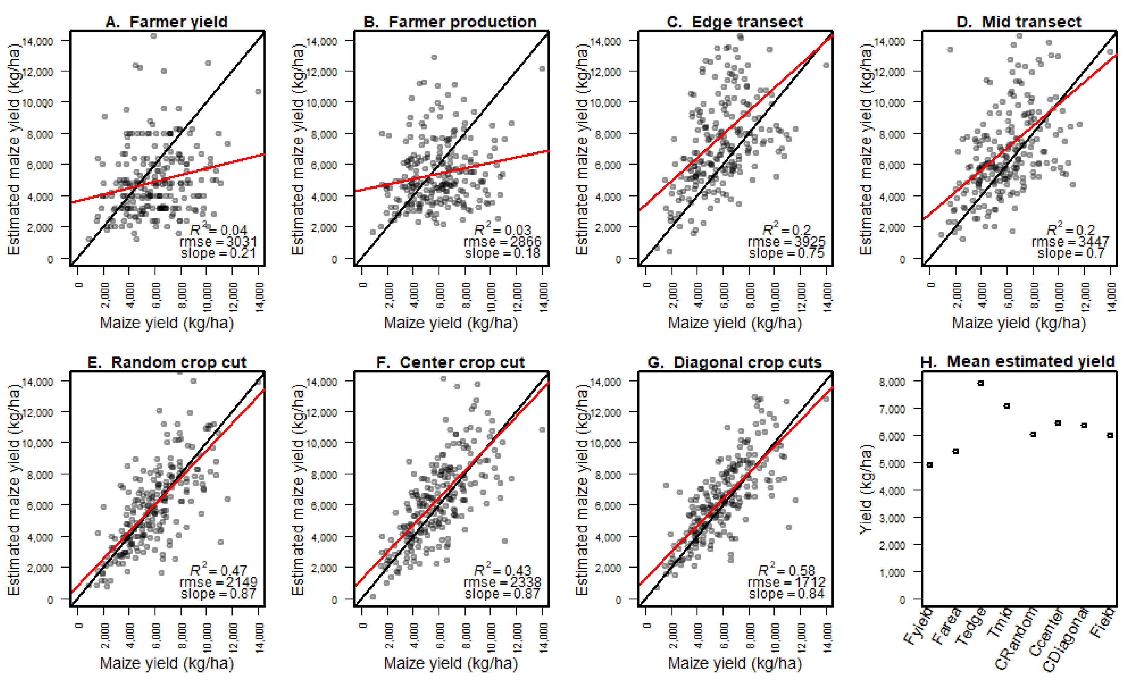
We compared models predicting maize yield from satellite reflectance data and field data from eight different yield measurement methods. We found that crop cut data accurately predicted full-field harvest data and that the models that used crop cut data were as accurate as those based on the full-field harvest data. We also found that crop cuts are highly cost-effective relative to other field methods to estimate crop yield. While farmer estimates were cheaper to obtain, they were only competitive with crop cuts at very small expenditures (<20 farmer estimates) and low accuracy. Our findings clearly indicated that for research under similar conditions, crop cuts should be used to build models to predict yield. The type of crop cut protocol used did not have a strong effect on model quality when using remote sensing to predict yield, but a single random location crop cut performed best. It was possible to obtain good results, on average, with relatively small sample sizes in the order of 30 crop cuts, but larger sample sizes improved the average accuracy and reduced the variability.

The transect methods performed poorly, and given that their costs are similar to crop cuts, there seems to be no good reason for using them, especially as it may be difficult to obtain an accurate plant density estimate with the transect methods. The advantage of the remote-sensing-based models relative to the NULL model (model gain) was relatively small even though we had a wide range of yield values. However, the gain was higher for crop cut methods, indicating that remote sensing is not a solution for fixing poor field data, but rather that it can further increase the value of good field data.

While taking multiple crop cuts per field gave a better direct estimate of yield, it did not lead to better remote sensing models than when using a single crop cut. This is unsurprising because the slope of the regression line between the crop cut yield estimate and the true yield was closer to one for the single crop cut data than for three crop cuts. Thus, while the better goodness of fit scores (R${}^2$ and RMSE) showed that the three crop cuts data were less noisy, the random location single-crop cut data were less biased—perhaps because the three cuts were taken along a diagonal. The ideal number of cuts and the size of the cuts should depend on in-field variability, and the results may also depend on the size of the cuts. The 16 m${}^2$ crop cut size has been used in other research [16,33]; however, smaller areas have also been used and the size can affect data quality. Given the high fixed cost of traveling to a field and obtaining permission to take a sample, we would recommend taking multiple cuts of at least 16 m${}^2$. Future work could evaluate the use of historical or in-season satellite data to estimate within-field variability to guide the amount and location of crop cuts.

The quality of farmer yield estimates may vary considerably by crop, region, and method employed. Our farmer estimates were elicited just prior to harvesting, rather than post-harvest, which is more commonly the case in survey data. Post-harvest estimates can be more accurate [34], as farmers will have observed and perhaps measured the amount harvested, for example through sales transactions. Farmers’ estimates of field size may be inaccurate, in particular due to rounding of the size of smaller fields [34]. However, we did not find a clear difference in crop yield estimates when using farmer estimates of both production and field size or only using farmer-estimated production combined with the researcher-determined field size. We found that farmers tended to underestimate yield, which is consistent with other studies (e.g., [14]). However, the most important shortcoming was that the relationship between the farmer estimate and the actual yield was very weak. Farmer yield estimates are commonly used in survey-based research, and our results suggest that a critical evaluation of their quality is important. Farmer estimates have been used to reconstruct time series of yield to support remote-sensing-based modeling for crop insurance [2,35]. It has been shown that with longer recall times, farmers tend to overestimate production and underestimate or forget the effect of marginally productive plots [36]. This suggests that farmer estimates may be more valid in a relative sense (bad and good years) than for absolute numbers.

The accuracy of our models was comparable with other studies of maize yield in East Africa [9,10,30]. However, our models are not directly comparable to studies that use additional predictor variables such as household size [34] and climatic variables [3,11]. We found that external accuracy was generally higher than internal accuracy, meaning that for most methods, the models predicted the full-field yield better than they predicted the estimated yield data on which the model was based. External accuracy being higher than internal accuracy was due to the noise (measurement error) in the sample-based field data used to evaluate the models, which led to an overestimation of the error. This implies that remote-sensing-based models may generally perform somewhat better than the reported (internal) cross-validation-based estimates suggest.

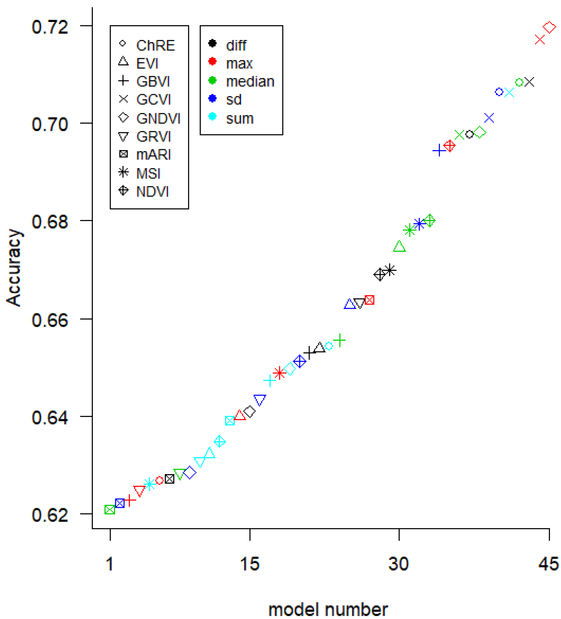
There was not a substantial difference in accuracy between the LR-1, LR-2, and RF modeling methods. However, the VI selected was important for accuracy. It has been reported that GCVI and Red edge VIs are useful in yield prediction for nitrogen-limited systems [9,24]. These VIs worked well with our data, though GNDVI performed best, in addition to GCVI and indices that used the Red edge, as reported by others [37]. The cumulative NDVI, which has been often used to predict yield, was one of the least accurate methods in our study. Many studies use the VI from a single date or a few dates [10] as the dependent variables in linear models of yield, due to the lack of available cloud-free imagery. More clarity is needed on what temporal aggregations to use and on the stability and generalizability of models based on a single date.

Model gain increased when using the remote sensing models to extrapolate, showing that the models had some degree of generality, making them useful for predicting in other (nearby) regions. Previous work indicated that the yield–VI relationship is very site-specific [38], and it is also dependent on the crop growth stage. We found that the differences between field methods were less pronounced for extrapolation between regions. Further study is needed to determine the generalizability of yield estimates from remote-sensing-based models across regions.

5. Conclusions

We found that crop cuts were an effective field method for estimating yield. Remote sensing models based on crop cut data generated predictions that were as accurate as those based on full-field harvest data, but at a much lower cost. Other methods did not perform well. Further work is needed to better understand the effect of different crop cut protocols and how well they perform under other conditions. There is also a need to better understand the best methods for predictor variable (VIs) selection and model fitting, especially in the context of extrapolation. Further development of accurate, low-cost yield predictions from high-quality field data and remote sensing data is a promising approach to filling data gaps on crop productivity in Sub-Saharan Africa and other data-sparse regions.

References

1. Eze, E.; Girma, A.; Zenebe, A.A.; Zenebe, G. Feasible crop insurance indexes for drought risk management in Northern Ethiopia. Int. J. Disaster Risk Reduct. 2020, 47, 101544. [Google Scholar] [CrossRef]
2. Benami, E.; Jin, Z.; Carter, M.R.; Ghosh, A.; Hijmans, R.J.; Hobbs, A.; Kenduiywo, B.; Lobell, D.B. Uniting remote sensing, crop modeling and economics for agricultural risk management. Nat. Rev. Earth Environ. 2021, 2, 140–159. [Google Scholar] [CrossRef]
3. Zinyengere, N.; Mhizha, T.; Mashonjowa, E.; Chipindu, B.; Geerts, S.; Raes, D. Using seasonal climate forecasts to improve maize production decision support in Zimbabwe. Agric. For. Meteorol. 2011, 151, 1792–1799. [Google Scholar] [CrossRef]
4. Delincé, J. Recent Practices and advances for AMIS Crop Yield Forecasting at Farm and Parcel Level: A Review; Food and Agriculture Organization of the United Nations: Rome, Italy, 2017. [Google Scholar]
5. Bonilla-Cedrez, C.; Chamberlin, J.; Hijmans, R.J. Fertilizer and grain prices constrain food production in sub-Saharan Africa. Nat. Food 2021, 2, 766–772. [Google Scholar] [CrossRef]
6. Fritz, S.; See, L.; Bayas, J.C.L.; Waldner, F.; Jacques, D.; Becker-Reshef, I.; Whitcraft, A.; Baruth, B.; Bonifacio, R.; Crutchfield, J.; et al. A comparison of global agricultural monitoring systems and current gaps. Agric. Syst. 2019, 168, 258–272. [Google Scholar] [CrossRef]
7. Lobell, D.B.; Di Tommaso, S.; You, C.; Yacoubou Djima, I.; Burke, M.; Kilic, T. Sight for sorghums: Comparisons of satellite-and ground-based sorghum yield estimates in mali. Remote Sens. 2020, 12, 100. [Google Scholar] [CrossRef] [Green Version]
8. Awad, M.M. Toward precision in crop yield estimation using remote sensing and optimization techniques. Agriculture 2019, 9, 54. [Google Scholar] [CrossRef] [Green Version]
9. Jin, Z.; Azzari, G.; You, C.; Di Tommaso, S.; Aston, S.; Burke, M.; Lobell, D.B. Smallholder maize area and yield mapping at national scales with Google Earth Engine. Remote Sens. Environ. 2019, 228, 115–128. [Google Scholar] [CrossRef]
10. Lobell, D.B.; Azzari, G.; Burke, M.; Gourlay, S.; Jin, Z.; Kilic, T.; Murray, S. Eyes in the Sky, Boots on the Ground: Assessing Satellite- and Ground-Based Approaches to Crop Yield Measurement and Analysis. Am. J. Agric. Econ. 2020, 102, 202–219. [Google Scholar] [CrossRef]
11. Prasad, A.K.; Chai, L.; Singh, R.P.; Kafatos, M. Crop yield estimation model for Iowa using remote sensing and surface parameters. Int. J. Appl. Earth Obs. Geoinf. 2006, 8, 26–33. [Google Scholar] [CrossRef]
12. Lima, J.d.J.A.d.; Maldaner, L.F.; Molin, J.P. Sensor fusion with narx neural network to predict the mass flow in a sugarcane harvester. Sensors 2021, 21, 4530. [Google Scholar] [CrossRef]
13. Maldaner, L.F.; de Paula Corrêdo, L.; Canata, T.F.; Molin, J.P. Predicting the sugarcane yield in real-time by harvester engine parameters and machine learning approaches. Comput. Electron. Agric. 2021, 181, 105945. [Google Scholar] [CrossRef]
14. Wahab, I. In-season plot area loss and implications for yield estimation in smallholder rainfed farming systems at the village level in Sub-Saharan Africa. GeoJournal 2020, 85, 1553–1572. [Google Scholar] [CrossRef] [Green Version]
15. Paliwal, A.; Jain, M. The Accuracy of Self-Reported Crop Yield Estimates and Their Ability to Train Remote Sensing Algorithms. Front. Sustain. Food Syst. 2020, 4, 1–10. [Google Scholar] [CrossRef] [Green Version]
16. Gourlay, S.; Kilic, T.; Lobell, D. Could the Debate Be Over? Errors in Farmer-Reported Production and Their Implications for the Inverse Scale-Productivity Relationship in Uganda; The World Bank: Washington, DC, USA, 2017. [Google Scholar]
17. Sapkota, T.B.; Jat, M.L.; Jat, R.K.; Kapoor, P.; Stirling, C. Yield Estimation of Food and Non-Food Crops in Smallholder Production Systems; Springer: Berlin/Heidelberg, Germnay, 2016; pp. 163–174. [Google Scholar] [CrossRef] [Green Version]
18. Diskin, P. Agricultural Productivity Indicators Measurement Guide; Food Security and Nutrition Monitoring (IMPACT) Project; IMPACT: Rome, Italy, 1997. [Google Scholar]
19. Buckland, S.T.; Borchers, D.L.; Johnston, A.; Henrys, P.A.; Marques, T.A. Line transect methods for plant surveys. Biometrics 2007, 63, 989–998. [Google Scholar] [CrossRef] [PubMed]
20. van de Voorde, T.F.; van der Putten, W.H.; Bezemer, T.M. The importance of plant–soil interactions, soil nutrients, and plant life history traits for the temporal dynamics of Jacobaea vulgaris in a chronosequence of old-fields. Oikos 2012, 121, 1251–1262. [Google Scholar] [CrossRef]
21. Kornher, L. Maize markets in Eastern and Southern Africa (ESA) in the context of climate change. In The State of Agricultural Commodity Markets (SOCO); FAO: Rome, Italy, 2018; Available online: https://www.fao.org/publications/card/en/c/CA2155EN/ (accessed on 10 April 2022).
22. Funk, C.; Budde, M.E. Phenologically-tuned MODIS NDVI-based production anomaly estimates for Zimbabwe. Remote Sens. Environ. 2009, 113, 115–125. [Google Scholar] [CrossRef]
23. Fernandez-Ordonez, Y.M.; Soria-Ruiz, J. Maize crop yield estimation with remote sensing and empirical models. Int. Geosci. Remote Sens. Symp. (IGARSS) 2017, 2017, 3035–3038. [Google Scholar] [CrossRef]
24. Lin, S.; Li, J.; Liu, Q.; Li, L.; Zhao, J.; Yu, W. Evaluating the Effectiveness of Using Vegetation Indices Based on Red-Edge Reflectance from Sentinel-2 to Estimate Gross Primary Productivity. Remote Sens. 2019, 11, 1303. [Google Scholar] [CrossRef] [Green Version]
25. Mirasi, A.; Mahmoudi, A.; Navid, H.; Valizadeh Kamran, K.; Asoodar, M.A. Evaluation of sum-NDVI values to estimate wheat grain yields using multi-temporal Landsat OLI data. Geocarto Int. 2019, 6049, 1–16. [Google Scholar] [CrossRef]
26. Peng, Y.; Gitelson, A.A. Application of chlorophyll-related vegetation indices for remote estimation of maize productivity. Agric. For. Meteorol. 2011, 151, 1267–1276. [Google Scholar] [CrossRef]
27. Sharma, L.K.; Bu, H.; Denton, A.; Franzen, D.W. Active-optical sensors using red NDVI compared to red edge NDVI for prediction of corn grain yield in north Dakota, U.S.A. Sensors 2015, 15, 27832–27853. [Google Scholar] [CrossRef] [PubMed]
28. Cui, Z.; Kerekes, J.P. Potential of red edge spectral bands in future landsat satellites on agroecosystem canopy green leaf area index retrieval. Remote Sens. 2018, 10, 1458. [Google Scholar] [CrossRef] [Green Version]
29. Prey, L.; Hu, Y.; Schmidhalter, U. High-Throughput Field Phenotyping Traits of Grain Yield Formation and Nitrogen Use Efficiency: Optimizing the Selection of Vegetation Indices and Growth Stages. Front. Plant Sci. 2020, 10, 1672. [Google Scholar] [CrossRef] [PubMed] [Green Version]
30. Burke, M.; Lobell, D.B. Satellite-based assessment of yield variation and its determinants in smallholder African systems. Proc. Natl. Acad. Sci. USA 2017, 114, 2189–2194. [Google Scholar] [CrossRef] [Green Version]
31. Lange, M.; Doktor, D. Phenex: Auxiliary Functions for Phenological Data Analysis; R Package Version 1.4-5; R Package Vignette: Madison, WI, USA, 2017. [Google Scholar]
32. Ghosh, A.; Mandel, A.K.B.; Hijmans, R. Luna: Tools for Satellite Remote Sensing (Earth Observation) Data Processing; R Package Version 0.3-2; R Package Vignette: Madison, WI, USA, 2020. [Google Scholar]
33. Kosmowski, F.; Ambel, A.; Tsegay, A.H.; Negawo, A.T.; Carling, J.; Kilian, A.; Agency, C.S. A large-scale dataset of barley, maize and sorghum variety identification using DNA fingerprinting in Ethiopia. Data 2021, 6, 58. [Google Scholar] [CrossRef]
34. Food and Agriculture Organization of the United States (FAO). Methodology for Estimation of Crop Area and Crop Yield under Mixed and Continuous Cropping; Technical Report; FAO: Rome, Italy, 2017. [Google Scholar]
35. Kenduiywo, B.K.; Carter, M.R.; Ghosh, A.; Hijmans, R.J. Evaluating the quality of remote sensing products for agricultural index insurance. PLoS ONE 2021, 16, e0258215. [Google Scholar] [CrossRef]
36. Wollburg, P.; Tiberti, M.; Zezza, A. Recall length and measurement error in agricultural surveys. Food Policy 2021, 100, 102003. [Google Scholar] [CrossRef]
37. Vallentin, C.; Harfenmeister, K.; Itzerott, S.; Kleinschmit, B.; Conrad, C.; Spengler, D. Suitability of satellite remote sensing data for yield estimation in northeast Germany. Precis. Agric. 2022, 23, 52–82. [Google Scholar] [CrossRef]
38. Turvey, C.G.; McLaurin, M.K. Applicability of the normalized difference vegetation index (NDVI) In index-based crop insurance design. Weather Clim. Soc. 2012, 4, 271–284. [Google Scholar] [CrossRef]
Figure 1. Maize yield (kg/ha) estimates from seven field sampling methods versus the true maize yield that was measured by harvesting the entire field. The black lines are the identity (y = x), and the red line is a linear regression model, with the associated adjusted R 2 displayed on each plot. The final panel shows the mean yield estimate by the sampling method; see Table 1.
Remotesensing 14 01995 g001
Figure 2. Internal and external accuracy and gain for models using data from 8 different field sampling methods to predicting maize yield with 1 or more of 45 Sentinel-2 reflectance-data-derived predictor variables. Single predictor variable (LR-1) and Random Forest (RF) (Panels (A,B); the Random Forest model is indicated with a + sign), and two-predictor-variable linear regression models (LR-2, Panels (C,D)).
Remotesensing 14 01995 g002
Figure 3. External accuracy vs. extrapolation accuracy and external gain vs. extrapolation gain for the yield prediction model that performed best in terms of external accuracy, for models based on data from eight field data collection methods (symbols) and three algorithms (colors).
Remotesensing 14 01995 g003
Figure 4. Maize yield prediction external accuracy for single-variable linear models (LR-1) using GNDVI-maximum as the predictor variable for four groupings of the eight field-based yield estimation techniques as a function of (A) sample size and (B) cost. Cost is expressed as a relative measure of effort where farmer estimates cost 1 unit and a full-field harvest is 35.6-times that amount of effort. Both sample size and relative cost are on a log-scale. Computed with Monte Carlo simulation (n = 200); the thick line is the median, and the dashed lines are the 0.05 and 0.95 quantiles. The values for the field estimation techniques were computed as the mean of their respective more disaggregated measures (see Table 1).
Remotesensing 14 01995 g004