
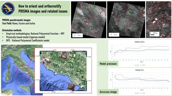
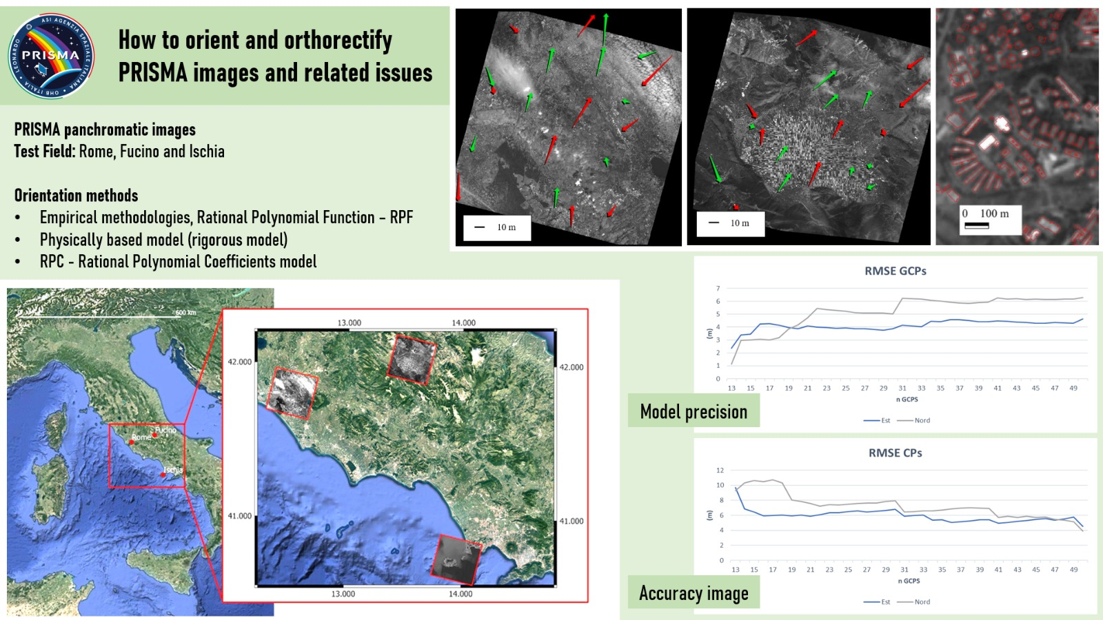
How to Orient and Orthorectify PRISMA Images and Related Issues


Abstract
:
1. Introduction
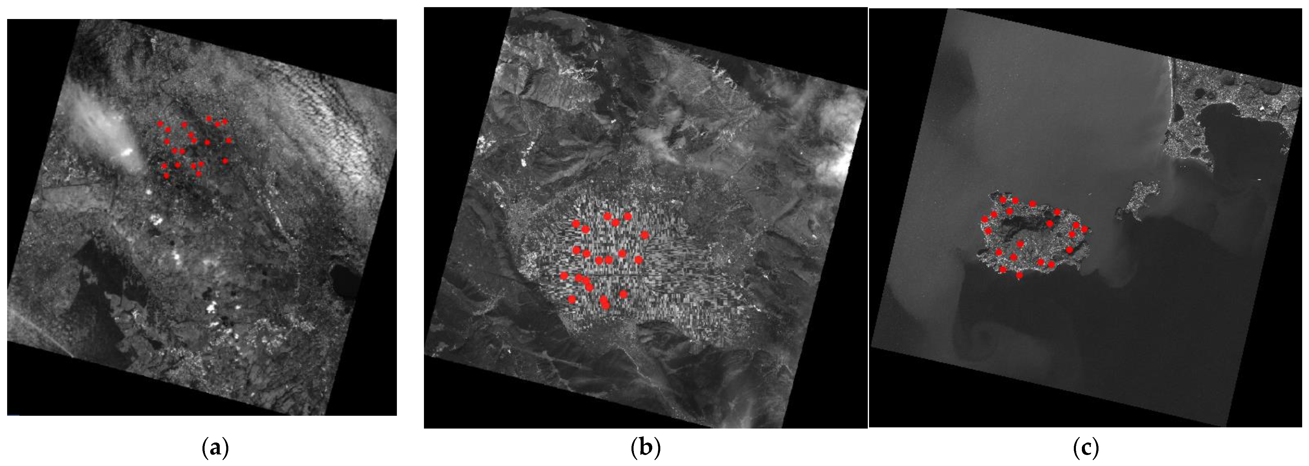
2. Materials and Methods
2.1. Export Procedure for Specific Bands and Related Issues
2.2. Orthorectification of PRISMA Images
3. Results and Discussion
3.1. Rigorous Model
3.1.1. Results of Rigorous Model

| Parameter | Value | Source |
|---|---|---|
| Across-track angle | 0.42 deg | Observing Angle |
| Along-track angle | 0 deg | Observing Angle |
| IFOV | 48 mrad | [32] |
| Altitude | 615 km | [30] |
| Period | 97 m | [30] |
| Semi-major axis | 6992.935 km | [31] |
| Eccentricity | 0.0011403 | [33] |
| Inclination | 97.851° | [32] |
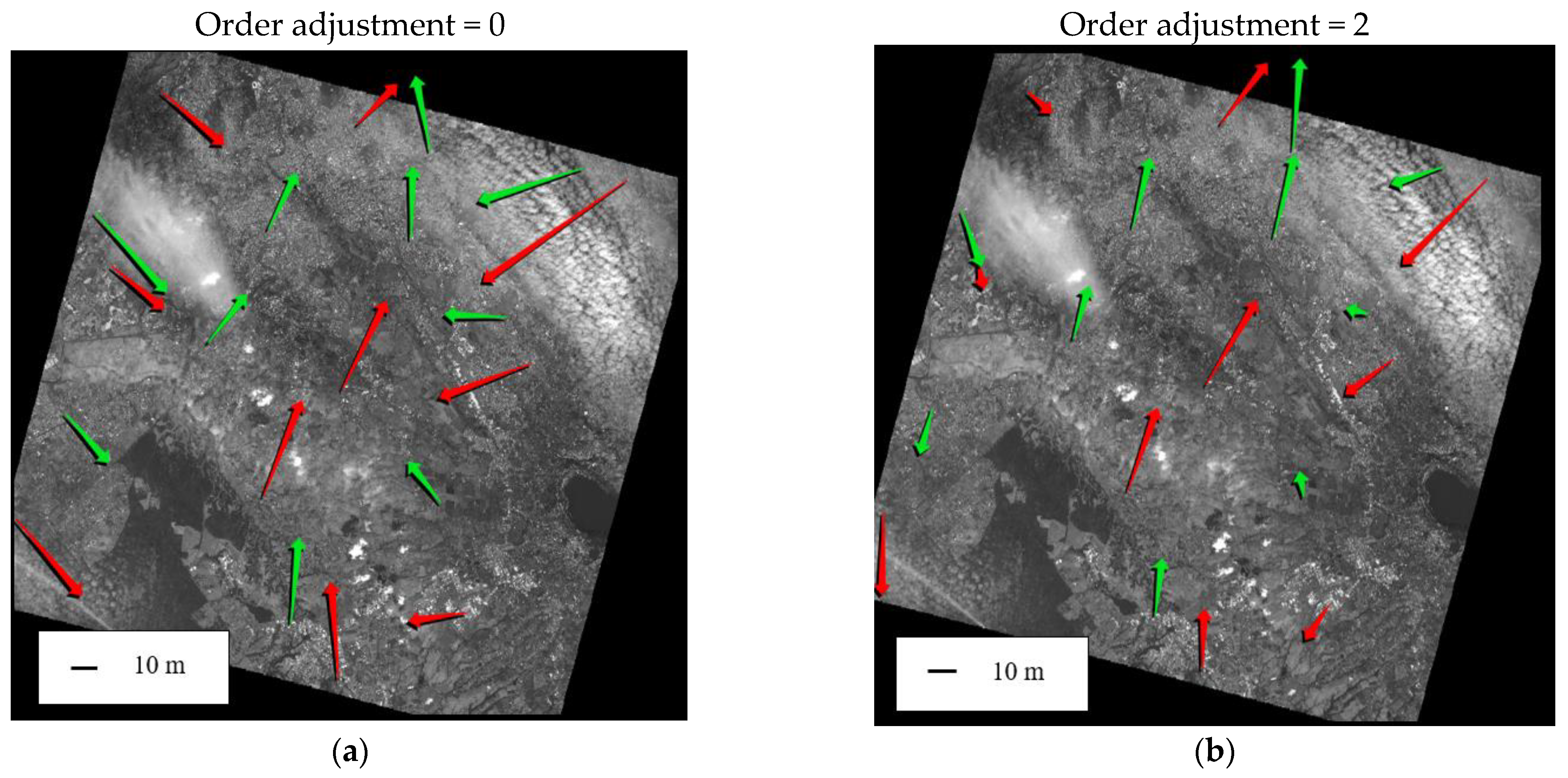
3.1.2. Discussion of Rigorous Model
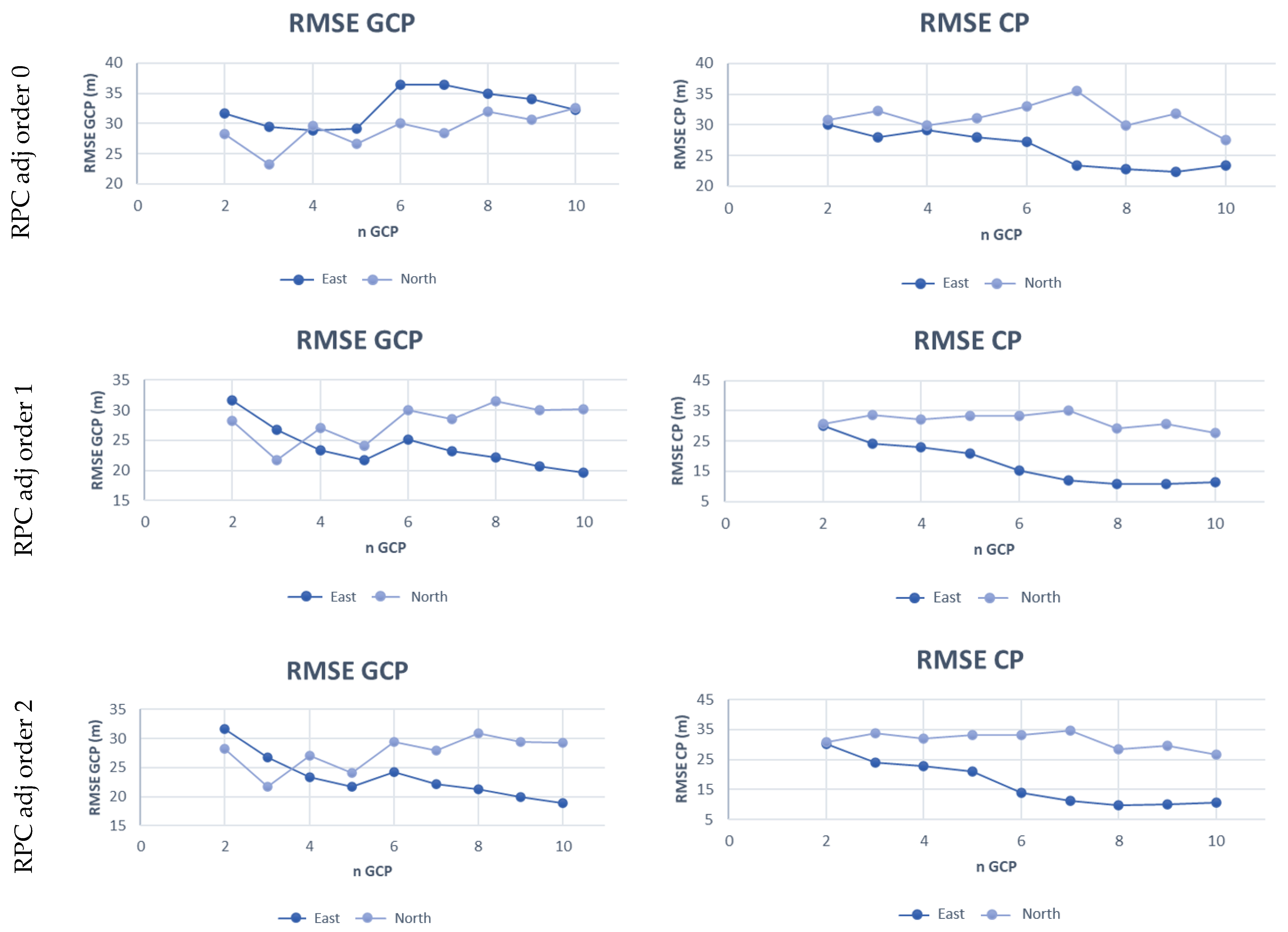
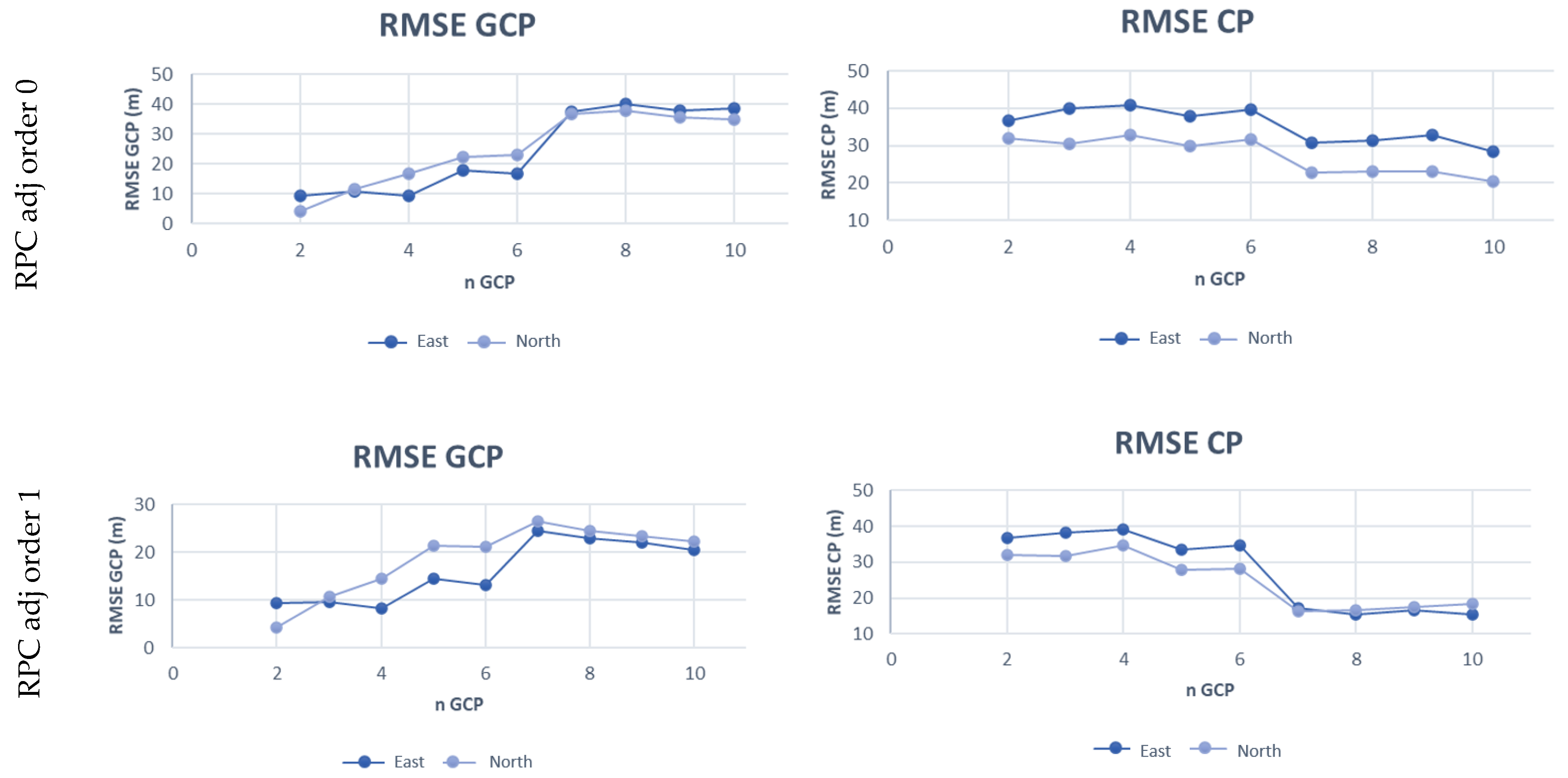
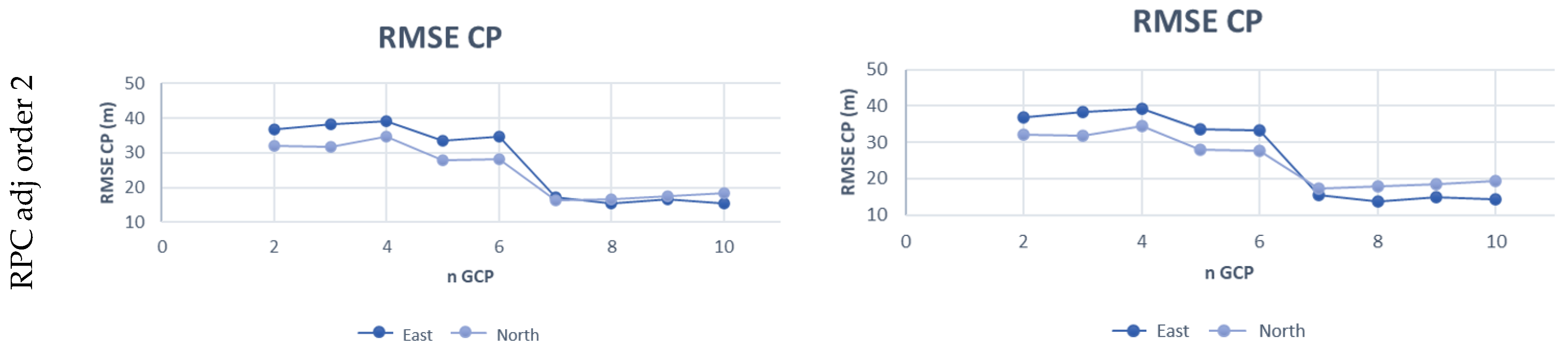
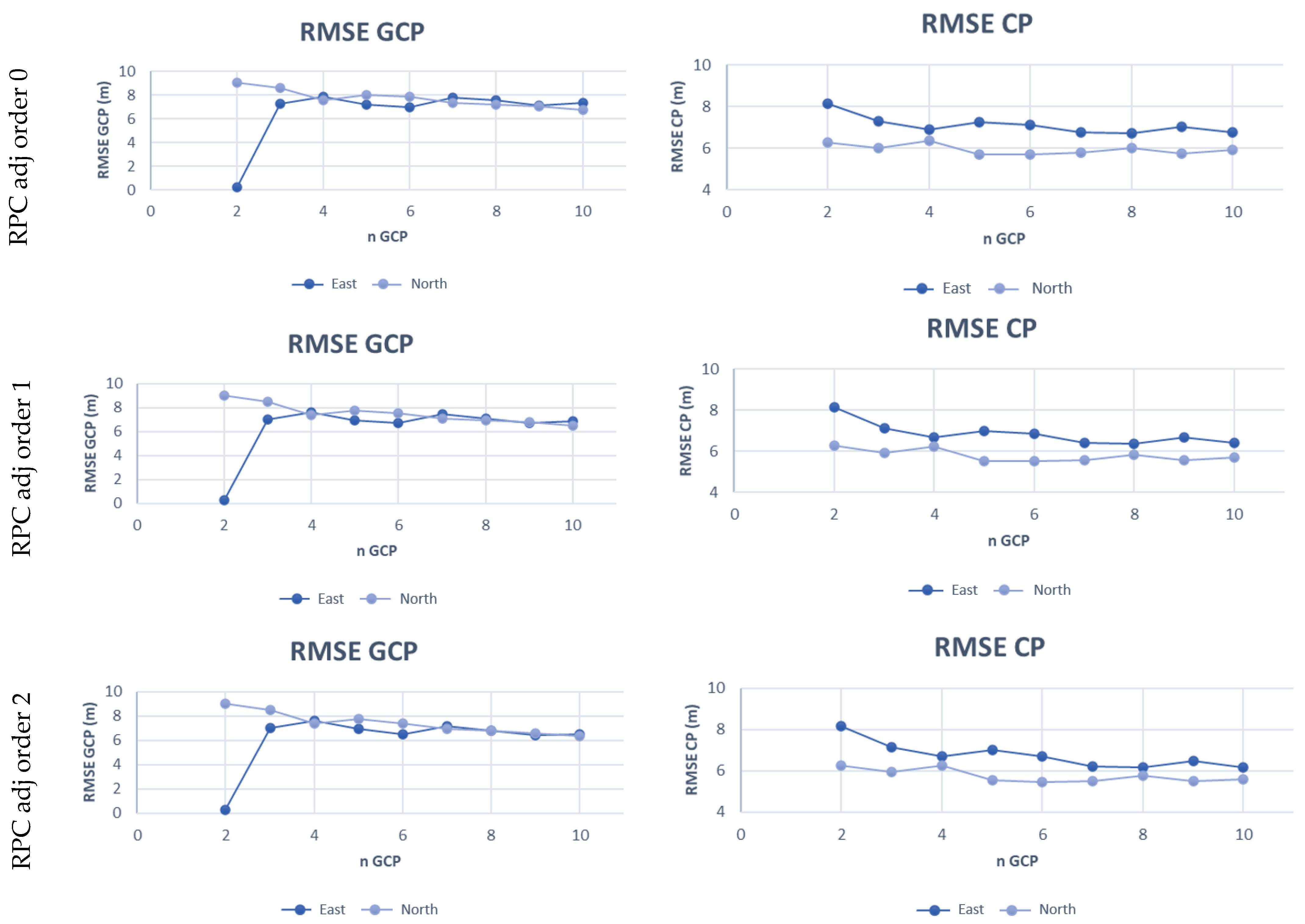
3.2. Results of RPC Model
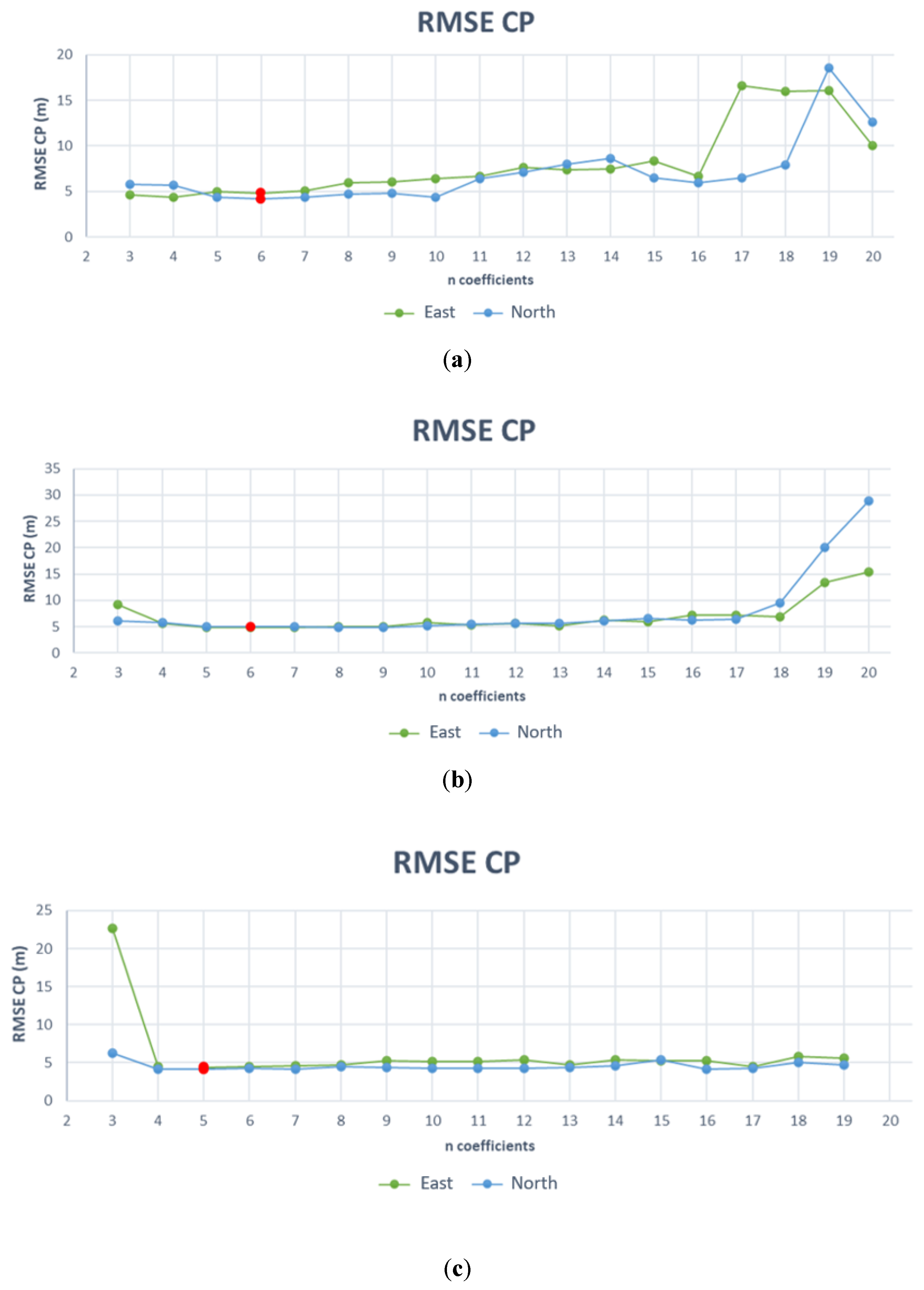
3.3. RPF Model
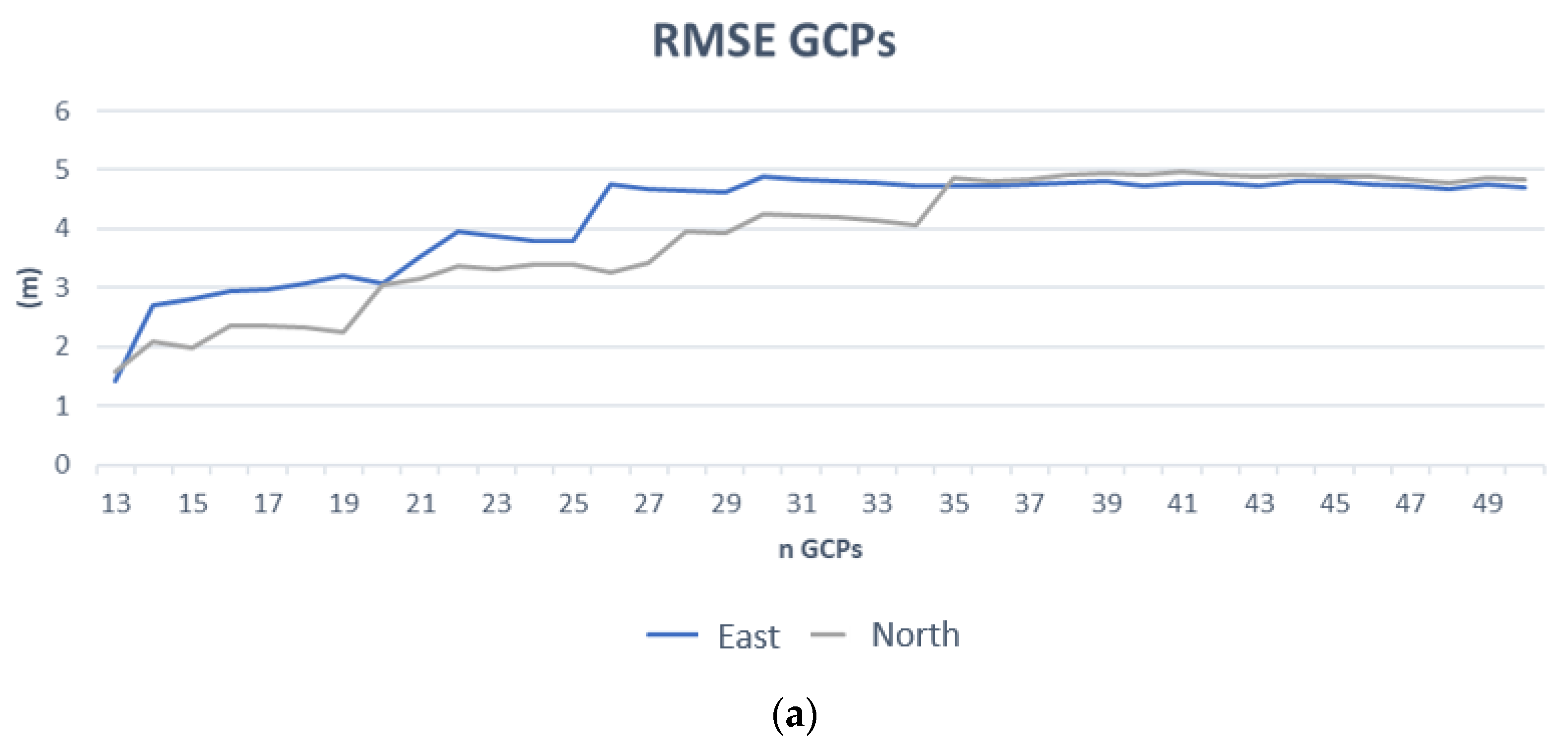
3.3.1. Results of RPF Model
3.3.2. Discussion of RPF Model
4. Conclusions
Author Contributions
Funding
Institutional Review Board Statement
Informed Consent Statement
Acknowledgments
Conflicts of Interest
Appendix A

| RPC Bundle Adjustment Solution | N. of GCPs (N. of CP) | RMSE Value of CP Discrepancies. Units Are in Metres | |
|---|---|---|---|
| E | N | ||
| Spatial Intersection | None (20) | 135.128 | 88.883 |
| RPC order 0: X0, Y0 | 2 (18) | 22.968 | 22.47 |
| RPC order 0: X0, Y0 | 7 (13) | 18134 | 23.208 |
| RPC order 1: X0, X1, X2, Y0, Y1, Y2 | 4 (16) | 14.668 | 23.068 |
| RPC order 1: X0, X1, X2, Y0, Y1, Y2 | 7 (13) | 12.96 | 23.177 |
| RPC order 1: X0, X1, X2, Y0, Y1, Y2 | 10 (10) | 9.139 | 22.769 |
| RPC order 2: X0, X1, X2, X3, X4, X5, Y0, Y1, Y2, Y3, Y4, Y5 | 7 (13) | 12.058 | 22.866 |
| RPC order 2: X0, X1, X2, X3, X4, X5, Y0, Y1, Y2, Y3, Y4, Y5 | 10 (10) | 8.106 | 22.467 |
| RPC Bundle Adjustment Solution | N. of GCPs (N. of CP) | RMSE Value of CP Discrepancies. Units Are in Metres | |
|---|---|---|---|
| E | N | ||
| Spatial Intersection | None (20) | 137.997 | 106.319 |
| RPC order 0: X0, Y0 | 2 (18) | 7.842 | 14.759 |
| RPC order 0: X0, Y0 | 7 (13) | 7.881 | 7.355 |
| RPC order 1: X0, X1, X2, Y0, Y1, Y2 | 4 (16) | 7.338 | 7.726 |
| RPC order 1: X0, X1, X2, Y0, Y1, Y2 | 7 (13) | 7.827 | 5.9 |
| RPC order 1: X0, X1, X2, Y0, Y1, Y2 | 10 (10) | 7.63 | 5.98 |
| RPC order 2: X0, X1, X2, X3, X4, X5, Y0, Y1, Y2, Y3, Y4, Y5 | 7 (13) | 7.836 | 5.824 |
| RPC order 2: X0, X1, X2, X3, X4, X5, Y0, Y1, Y2, Y3, Y4, Y5 | 10 (10) | 7.722 | 5.809 |
| RPC Bundle Adjustment Solution | N. of GCPs (N. of CP) | RMSE Value of CP Discrepancies. Units Are in Metres | |
|---|---|---|---|
| E | N | ||
| Spatial Intersection | None (20) | 156.498 | 57.906 |
| RPC order 0: X0, Y0 | 2 (18) | 5.911 | 21.938 |
| RPC order 0: X0, Y0 | 7 (13) | 5.719 | 19.891 |
| RPC order 1: X0, X1, X2, Y0, Y1, Y2 | 4 (16) | 6.422 | 26.909 |
| RPC order 1: X0, X1, X2, Y0, Y1, Y2 | 7 (13) | 5.601 | 19.708 |
| RPC order 1: X0, X1, X2, Y0, Y1, Y2 | 10 (10) | 6.017 | 20.066 |
| RPC order 2: X0, X1, X2, X3, X4, X5, Y0, Y1, Y2, Y3, Y4, Y5 | 7 (13) | 5.461 | 19.254 |
| RPC order 2: X0, X1, X2, X3, X4, X5, Y0, Y1, Y2, Y3, Y4, Y5 | 10 (10) | 5.854 | 19.507 |
| RPC Bundle Adjustment Solution | N. of GCPs (N. of CP) | RMSE Value of CP Discrepancies. Units Are in Metres | |
|---|---|---|---|
| E | N | ||
| Spatial Intersection | None (20) | 61.103 | 30.784 |
| RPC order 0: X0, Y0 | 2 (18) | 22.488 | 21.314 |
| RPC order 0: X0, Y0 | 7 (13) | 17.95 | 18.11 |
| RPC order 1: X0, X1, X2, Y0, Y1, Y2 | 4 (16) | 20.433 | 18.245 |
| RPC order 1: X0, X1, X2, Y0, Y1, Y2 | 7 (13) | 18.934 | 17.415 |
| RPC order 1: X0, X1, X2, Y0, Y1, Y2 | 10 (10) | 17.157 | 17.141 |
| RPC order 2: X0, X1, X2, X3, X4, X5, Y0, Y1, Y2, Y3, Y4, Y5 | 7 (13) | 19.231 | 17.627 |
| RPC order 2: X0, X1, X2, X3, X4, X5, Y0, Y1, Y2, Y3, Y4, Y5 | 10 (10) | 17.212 | 17.099 |

| RPC Bundle Adjustment Solution | N. of GCPs (N. of CP) | RMSE value of CP Discrepancies. Units Are in Metres | |
|---|---|---|---|
| E | N | ||
| Spatial Intersection | None (20) | 145.989 | 99.858 |
| RPC order 0: X0, Y0 | 2 (18) | 5.439 | 14.128 |
| RPC order 0: X0, Y0 | 7 (13) | 5.478 | 15.798 |
| RPC order 1: X0, X1, X2, Y0, Y1, Y2 | 4 (16) | 5.359 | 11.891 |
| RPC order 1: X0, X1, X2, Y0, Y1, Y2 | 7 (13) | 5.365 | 12.217 |
| RPC order 1: X0, X1, X2, Y0, Y1, Y2 | 10 (10) | 4.759 | 11.402 |
| RPC order 2: X0, X1, X2, X3, X4, X5, Y0, Y1, Y2, Y3, Y4, Y5 | 7 (13) | 5.317 | 11.414 |
| RPC order 2: X0, X1, X2, X3, X4, X5, Y0, Y1, Y2, Y3, Y4, Y5 | 10 (10) | 4.833 | 10.582 |
| RPC Bundle Adjustment Solution | N. of GCPs (N. of CP) | RMSE Value of CP Discrepancies. Units Are in Metres | |
|---|---|---|---|
| E | N | ||
| Spatial Intersection | None (20) | 158.24 | 71.255 |
| RPC order 0: X0, Y0 | 2 (18) | 11.925 | 24.684 |
| RPC order 0: X0, Y0 | 7 (13) | 9.409 | 26.421 |
| RPC order 1: X0, X1, X2, Y0, Y1, Y2 | 4 (16) | 11.043 | 22.122 |
| RPC order 1: X0, X1, X2, Y0, Y1, Y2 | 7 (13) | 8.672 | 24.179 |
| RPC order 1: X0, X1, X2, Y0, Y1, Y2 | 10 (10) | 8.37 | 21.756 |
| RPC order 2: X0, X1, X2, X3, X4, X5, Y0, Y1, Y2, Y3, Y4, Y5 | 7 (13) | 8.818 | 23.152 |
| RPC order 2: X0, X1, X2, X3, X4, X5, Y0, Y1, Y2, Y3, Y4, Y5 | 10 (10) | 8.667 | 20.454 |
| RPC Bundle Adjustment Solution | N. of GCPs (N. of CP) | RMSE Value of CP Discrepancies. Units Are in Metres | |
|---|---|---|---|
| E | N | ||
| Spatial Intersection | None (20) | 66.662 | 32.143 |
| RPC order 0: X0, Y0 | 2 (18) | 21.436 | 29.653 |
| RPC order 0: X0, Y0 | 7 (13) | 18.004 | 17.514 |
| RPC order 1: X0, X1, X2, Y0, Y1, Y2 | 4 (16) | 17.631 | 20.029 |
| RPC order 1: X0, X1, X2, Y0, Y1, Y2 | 7 (13) | 17.41 | 16.395 |
| RPC order 1: X0, X1, X2, Y0, Y1, Y2 | 10 (10) | 17.071 | 15.243 |
| RPC order 2: X0, X1, X2, X3, X4, X5, Y0, Y1, Y2, Y3, Y4, Y5 | 7 (13) | 17.369 | 16.287 |
| RPC order 2: X0, X1, X2, X3, X4, X5, Y0, Y1, Y2, Y3, Y4, Y5 | 10 (10) | 17.022 | 15.102 |
References
- Koçal, A.; Duzgun, H.S.; Karpuz, C. Discontinuity Mapping with Automatic Lineament Extraction from High Resolution Satellite Imagery; ISPRS XX: Istanbul, Turkey, 2004; pp. 12–23. [Google Scholar]
- Chen, T.; Trinder, J.C.; Niu, R. Object-Oriented Landslide Mapping Using ZY-3 Satellite Imagery, Random Forest and Mathematical Morphology, for the Three-Gorges Reservoir, China. Remote Sens. 2017, 9, 333. [Google Scholar] [CrossRef] [Green Version]
- Lu, H.; Ma, L.; Fu, X.; Liu, C.; Wang, Z.; Tang, M.; Li, N. Landslides Information Extraction Using Object-Oriented Image Analysis Paradigm Based on Deep Learning and Transfer Learning. Remote Sens. 2020, 12, 752. [Google Scholar] [CrossRef] [Green Version]
- Rostami, M.; Kolouri, S.; Eaton, E.; Kim, K. Deep Transfer Learning for Few-Shot SAR Image Classification. Remote Sens. 2019, 11, 1374. [Google Scholar] [CrossRef] [Green Version]
- Baiocchi, V.; Brigante, R.; Dominici, D.; Milone, M.V.; Mormile, M.; Radicioni, F. Automatic three-dimensional features extraction: The case study of L’Aquila for collapse identification after April 06, 2009 earthquake. Eur. J. Remote Sens. 2014, 47, 413–435. [Google Scholar] [CrossRef]
- Transon, J.; D’Andrimont, R.; Maugnard, A.; Defourny, P. Survey of Hyperspectral Earth Observation Applications from Space in the Sentinel-2 Context. Remote Sens. 2018, 10, 157. [Google Scholar] [CrossRef] [Green Version]
- Pignatti, S.; Acito, N.; Amato, U.; Casa, R.; Bonis, R.d.; Diani, M.; Laneve, G.; Matteoli, S.; Palombo, A.; Pascucci, S.; et al. Development of algorithms and products for supporting the Italian hyperspectral PRISMA mission: The SAP4PRISMA project. In Proceedings of the 2012 IEEE International Geoscience and Remote Sensing Symposium, Munich, Germany, 22–27 July 2012; pp. 127–130. [Google Scholar]
- Guarini, R.; Loizzo, R.; Facchinetti, C.; Longo, F.; Ponticelli, B.; Faraci, M.; Dami, M.; Cosi, M.; Amoruso, L.; de Pasquale, V.; et al. Prisma Hyperspectral Mission Products. In Proceedings of the IEEE International Geoscience and Remote Sensing Symposium, IGARSS ’18, Valencia, Spain, 22–27 July 2018; pp. 179–182. [Google Scholar]
- Loizzo, R.; Daraio, M.; Guarini, R.; Longo, F.; Lorusso, R.; Dini, L.; Lopinto, E. Prisma Mission Status and Perspective. In Proceedings of the IEEE International Geoscience and Remote Sensing Symposium, IGARSS ’19, Yokohama, Japan, 28 July–2 August 2019; pp. 4503–4506. [Google Scholar]
- Giardino, C.; Bresciani, M.; Braga, F.; Fabbretto, A.; Ghirardi, N.; Pepe, M.; Gianinetto, M.; Colombo, R.; Cogliati, S.; Ghebrehiwot, S.; et al. First Evaluation of PRISMA Level 1 Data for Water Applications. Sensors 2020, 20, 4553. [Google Scholar] [CrossRef] [PubMed]
- Vangi, E.; D’Amico, G.; Francini, S.; Giannetti, F.; Lasserre, B.; Marchetti, M.; Chirici, G. The New Hyperspectral Satellite PRISMA: Imagery for Forest Types Discrimination. Sensors 2021, 21, 1182. [Google Scholar] [CrossRef] [PubMed]
- Busetto, L.; Ranghetti, L. Prismaread: A Tool for Facilitating Access and Analysis of PRISMA L1/L2 Hyperspectral Imagery v1.0.0. 2020. Available online: https://lbusett.github.io/prismaread/ (accessed on 22 February 2022).
- Toutin, T. Review article: Geometric processing of remote sensing images: Models, algorithms and methods. Int. J. Remote Sens. 2004, 25, 1893–1924. [Google Scholar] [CrossRef]
- Poli, D. A Rigorous Model for Spaceborne Linear Array Sensors. Photogramm. Eng. Remote Sens. 2007, 73, 187–196. [Google Scholar] [CrossRef] [Green Version]
- Mikhail, E.M.; Bethel, J.S.; McGlone, J.C. Introduction to Modern Photogrammetry; Wiley: Hoboken, NJ, USA, 2001; ISBN 978-0-471-30924-6. [Google Scholar]
- Fraser, C.S.; Hanley, H.B. Bias-compensated RPCs for Sensor Orientation of High-resolution Satellite Imagery. Photogramm. Eng. Remote Sens. 2005, 71, 909–915. [Google Scholar] [CrossRef]
- Tong, X.; Liu, S.; Weng, Q. Bias-corrected rational polynomial coefficients for high accuracy geo-positioning of QuickBird stereo imagery. ISPRS J. Photogramm. Remote Sens. 2010, 65, 218–226. [Google Scholar] [CrossRef]
- Meguro, Y.; Fraser, C.S. Georeferencing accuracy of Geoeye-1 stereo imagery: Experiences in a Japanese test field. Int. Arch. Photogramm. Remote Sens. Spat. Inf. Sci. 2010, 38, 1069–1072. [Google Scholar]
- Poli, D.; Toutin, T. Review of developments in geometric modelling for high resolution satellite pushbroom sensors. Photogramm. Rec. 2012, 27, 58–73. [Google Scholar] [CrossRef]
- Rupnik, E.; Deseilligny, M.P.; Delorme, A.; Klinger, Y. Refined satellite image orientation in the free open-source photogrammetric tools apero/micmac. ISPRS Ann. Photogramm. Remote Sens. Spat. Inf. Sci. 2016, III-1, 83–90. [Google Scholar] [CrossRef] [Green Version]
- Hanley, H.B.; Fraser, C.S. Sensor orientation for high-resolution satellite imagery: Further insights into bias-compensated RPCs. Photogramm. Eng. Remote Sens. 2004, 71. Available online: https://www.researchgate.net/publication/228806391_Sensor_orientation_for_high-resolution_satellite_imagery_Further_insights_into_bias-compensated_RPCs (accessed on 22 February 2022).
- Jacobsen, K. Systematic geometric image errors of very high resolution optical satellites. ISPRS Int. Arch. Photogramm. Remote Sens. Spat. Inf. Sci. 2018, XLII-1, 233–238. [Google Scholar] [CrossRef] [Green Version]
- Zhou, G.; Li, R. Accuracy Evaluation of Ground Points from IKONOS High-Resolution Satellite imagery. Photogramm. Eng. Remote. Sens. 2000, 66, 1103–1112. [Google Scholar]
- Baiocchi, V.; Giannone, F.; Monti, F.; Vatore, F. ACYOTB plugin: Tool for accurate orthorectification in open-source environments. ISPRS Int. J. Geo Inf. 2019, 9, 11. [Google Scholar] [CrossRef] [Green Version]
- Poli, D.; Remondino, F.; Angiuli, E.; Agugiaro, G. Radiometric and geometric evaluation of GeoEye-1, WorldView-2 and Pléiades-1A stereo images for 3D information extraction. ISPRS J. Photogramm. Remote Sens. 2015, 100, 35–47. [Google Scholar] [CrossRef]
- Agugiaro, G.; Poli, D.; Remondino, F. Testfield Trento: Geometric Evaluation Of Very High Resolution Satellite Imagery. ISPRS Int. Arch. Photogramm. Remote Sens. Spat. Inf. Sci. 2012, XXXIX-B1, 191–196. [Google Scholar] [CrossRef] [Green Version]
- Zheng, X.; Huang, Q.; Wang, J.; Wang, T.; Zhang, G. Geometric Accuracy Evaluation of High-Resolution Satellite Images Based on Xianning Test Field. Sensors 2018, 18, 2121. [Google Scholar] [CrossRef] [PubMed] [Green Version]
- Tarquini, S.; Isola, I.; Favalli, M.; Battistini, A. TINITALY, a Digital Elevation Model of Italy with a 10 Meters Cell Size (Version 1.0) [Data Set]; Istituto Nazionale di Geofisica e Vulcanologia (INGV): Rome, Italy, 2007. [CrossRef]
- National Imagery and Mapping Agency. “The Compendium of Controlled Extensions (CE) for the National Imagery Transmission Format (NITF)”, VERSION 2.1, 16 November 2000. Available online: http://geotiff.maptools.org/STDI-0002_v2.1.pdf (accessed on 22 February 2022).
- Loizzo, R.; Ananasso, C.; Guarini, R.; Lopinto, E.; Candela, L.; Pisani, A.R. The prisma hyperspectral mission. In Proceedings of the Living Planet Symposium, Prague, Czech Republic, 9–13 May 2016; pp. 9–13. [Google Scholar]
- PRISMA: La Missione Iperspettrale Nazionale, Conferenza 2018. Available online: http://conferenzecisam.it/convegni/c-i-s-a-m-2018-1/documenti/Loizzo_PRISMA%20La%20missione%20iperspettrale%20nazionale.pdf (accessed on 22 February 2022).
- IFAC CNR, Progetto Optima. 2014. Available online: http://www.ifac.cnr.it/corsari/meteors/private/OPTIMA%20-%20PRISMA%20Products%20and%20Applications%20-%20140930.pdf (accessed on 22 February 2022).
- Guarini, R.; Loizzo, R.; Longo, F.; Mari, S.; Scopa, T.; Varacalli, G. Overview of the PRISMA space and ground segment and its hyperspectral products. In Proceedings of the IEEE International Geoscience and Remote Sensing Symposium (IGARSS), Fort Worth, TX, USA, 23–28 July 2017; pp. 431–434. [Google Scholar] [CrossRef]

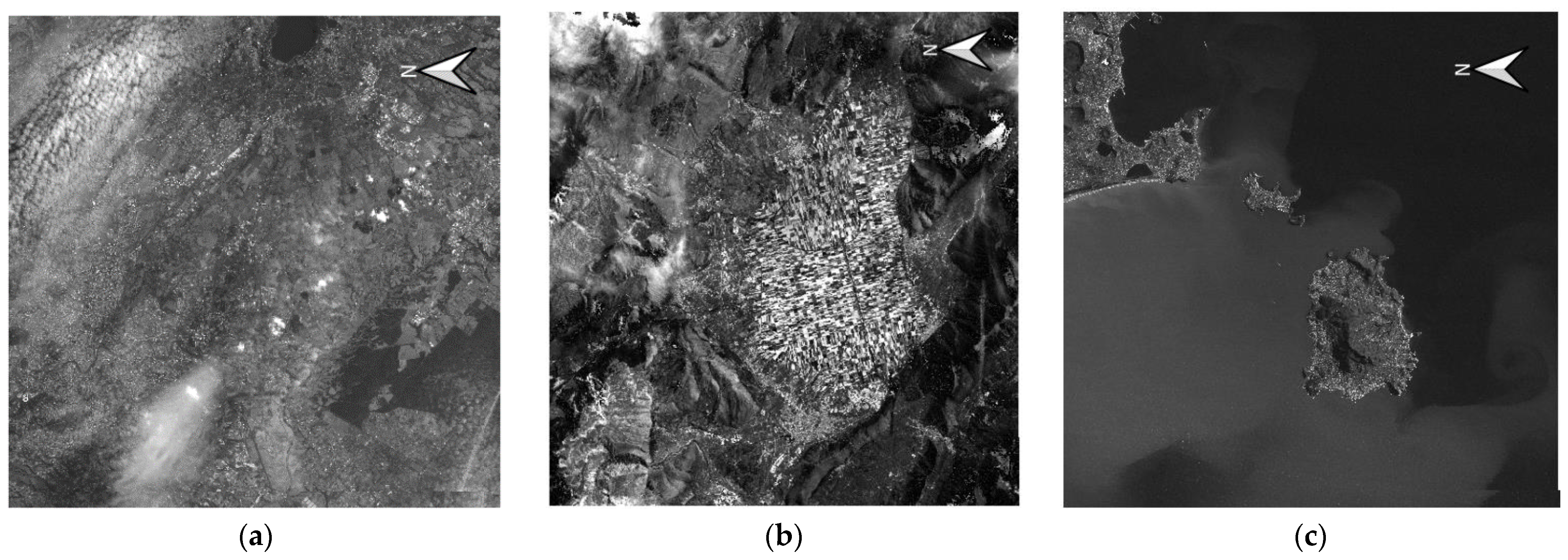


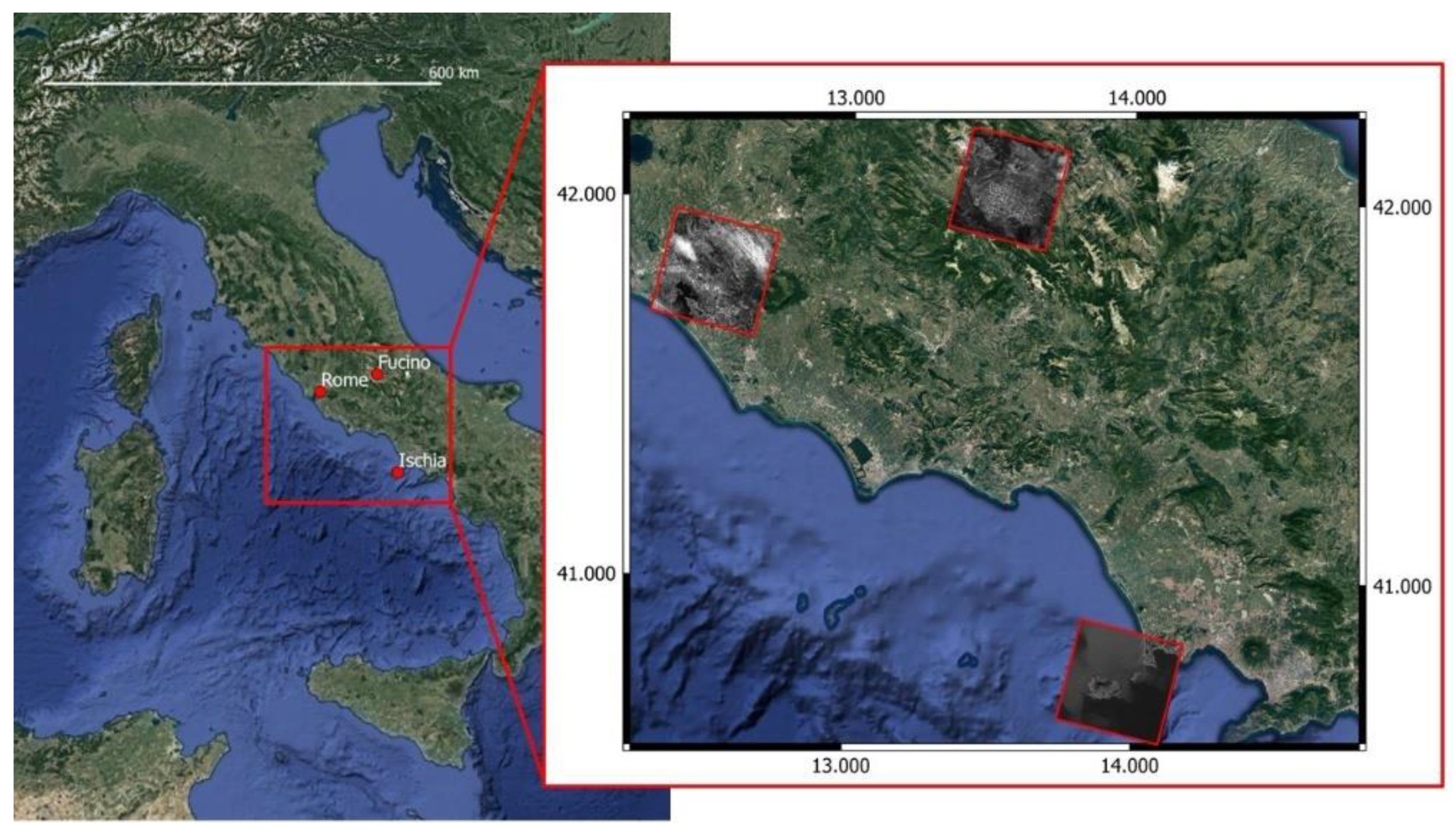
| Test Field | Approximate Range of Orthometric Heights | View Zenith Angle | Geomorphology and Notable Features |
|---|---|---|---|
| Rome | 0 to 596 m | 0.420° | Low relief and mountainous area |
| Fucino | 500 m to 2475 m | 1.459° | Mountainous terrain |
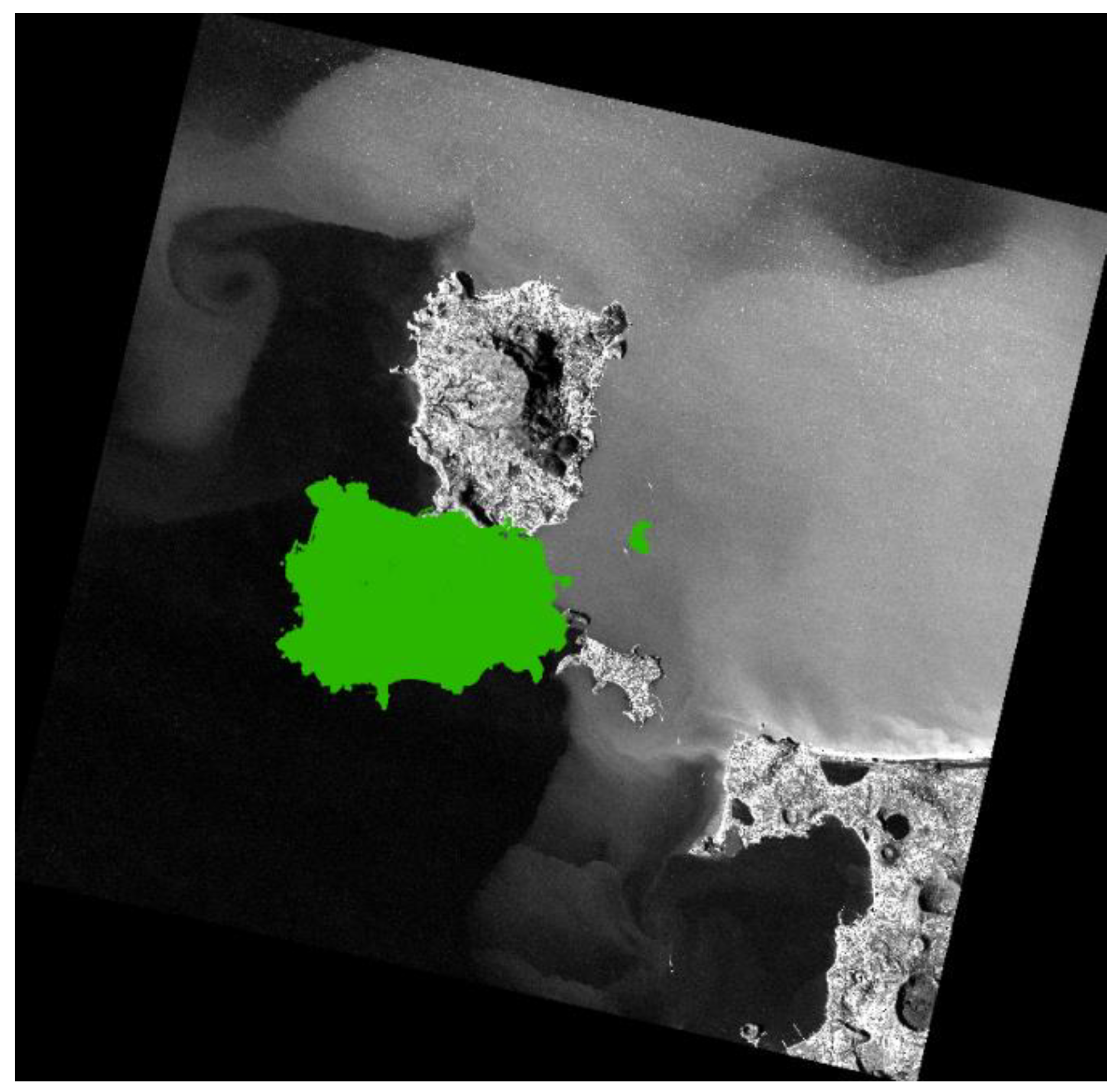
| Ischia | 0 to 777 m | 12.435° | Mountainous terrain appears only in the central part of the whole image |
| RPC Parameters | Min Number of GCPs | |
|---|---|---|
| RPC adjustment order = 0 | X0, Y0 | 1 |
| RPC adjustment order = 1 | X0, X1, X2, Y0, Y1, Y2 | 3 |
| RPC adjustment order = 2 | X0, X1, X2, X3, X4, X5, Y0, Y1, Y2, Y3, Y4, Y5 | 6 |
| N. of GCPs (N. of CP) | RMSE Value of Ground Checkpoint Discrepancies. Units Are in Metres | |
|---|---|---|
| E | N | |
| 7 GCP | 13.322 | 30.662 |
| 10 GCP | 13.699 | 27.117 |
| 15 GCP | 12.533 | 23.704 |
| 20 GCP | 12.925 | 22.046 |
| RPC Bundle Adjustment Solution | N. of GCPs (N. of CP) | RMSE Value of CP Discrepancies. Units Are in Metres | |
|---|---|---|---|
| E | N | ||
| Spatial Intersection | None (20) | 59.43 | 35.922 |
| RPC order 0: X0, Y0 | 2 (18) | 8.156 | 6.268 |
| RPC order 0: X0, Y0 | 7 (13) | 7.821 | 5.766 |
| RPC order 1: X0, X1, X2, Y0, Y1,Y2 | 4 (16) | 6.697 | 6.257 |
| RPC order 1: X0, X1, X2, Y0, Y1,Y2 | 7 (13) | 6.434 | 5.586 |
| RPC order 1: X0, X1, X2, Y0, Y1,Y2 | 10 (10) | 6.397 | 5.703 |
| RPC order 2: X0, X1, X2, X3, X4, X5, Y0, Y1, Y2, Y3, Y4, Y5 | 7 (13) | 5.489 | 5.489 |
| RPC order 2: X0, X1, X2, X3, X4, X5, Y0, Y1, Y2, Y3, Y4, Y5 | 10 (10) | 6.183 | 5.593 |
| RPC Bundle Adjustment Solution | N. of GCPs (N. of CP) | RMSE Value of CP Discrepancies. Units Are in Metres | |
|---|---|---|---|
| E | N | ||
| Spatial Intersection | None (20) | 130.762 | 80.972 |
| RPC order 0: X0, Y0 | 2 (18) | 30.077 | 30.783 |
| RPC order 0: X0, Y0 | 7 (13) | 23.423 | 35.518 |
| RPC order 1: X0, X1, X2, Y0, Y1, Y2 | 4 (16) | 22.884 | 32 |
| RPC order 1: X0, X1, X2, Y0, Y1, Y2 | 7 (13) | 12.004 | 35.091 |
| RPC order 1: X0, X1, X2, Y0, Y1, Y2 | 10 (10) | 11.368 | 27.62 |
| RPC order 2: X0, X1, X2, X3, X4, X5, Y0, Y1, Y2, Y3, Y4, Y5 | 7 (13) | 11.173 | 34.684 |
| RPC order 2: X0, X1, X2, X3, X4, X5, Y0, Y1, Y2, Y3, Y4, Y5 | 10 (10) | 10.553 | 26.68 |
| RPC Bundle Adjustment Solution | N. of GCPs (N. of CP) | RMSE Value of CP Discrepancies. Units Are in Metres | |
|---|---|---|---|
| E | N | ||
| Spatial Intersection | None (20) | 127.618 | 83.365 |
| RPC order 0: X0, Y0 | 2 (18) | 36.77 | 32.052 |
| RPC order 0: X0, Y0 | 7 (13) | 30.873 | 22.698 |
| RPC order 1: X0, X1, X2, Y0, Y1, Y2 | 4 (16) | 39.267 | 34.575 |
| RPC order 1: X0, X1, X2, Y0, Y1, Y2 | 7 (13) | 17.276 | 16.441 |
| RPC order 1: X0, X1, X2, Y0, Y1, Y2 | 10 (10) | 15.31 | 18.439 |
| RPC order 2: X0, X1, X2, X3, X4, X5, Y0, Y1, Y2, Y3, Y4, Y5 | 7 (13) | 15.38 | 17.263 |
| RPC order 2: X0, X1, X2, X3, X4, X5, Y0, Y1, Y2, Y3, Y4, Y5 | 10 (10) | 14.46 | 19.386 |
| RPC Bundle Adjustment Solution | N. of GCPs (N. of CP) | RMSE Value of CP Discrepancies. Units Are in Metres | |
|---|---|---|---|
| E | N | ||
| Spatial Intersection | None (20) | 138.763 | 102.29 |
| RPC order 0: X0, Y0 | 2 (18) | 5.857 | 5.231 |
| RPC order 0: X0, Y0 | 7 (13) | 4.361 | 4.68 |
| RPC order 1: X0, X1, X2, Y0, Y1, Y2 | 4 (16) | 4.234 | 5.847 |
| RPC order 1: X0, X1, X2, Y0, Y1, Y2 | 7 (13) | 4.335 | 4.753 |
| RPC order 1: X0, X1, X2, Y0, Y1, Y2 | 10 (10) | 3.168 | 4.99 |
| RPC order 2: X0, X1, X2, X3, X4, X5, Y0, Y1, Y2, Y3, Y4, Y5 | 7 (13) | 4.325 | 4.786 |
| RPC order 2: X0, X1, X2, X3, X4, X5, Y0, Y1, Y2, Y3, Y4, Y5 | 10 (10) | 3.157 | 5.014 |
| RPC Bundle Adjustment Solution | N. of GCPs (N. of CP) | RMSE Value of CP Discrepancies. Units Are in Metres | |
|---|---|---|---|
| E | N | ||
| Spatial Intersection | None (20) | 144.924 | 108.254 |
| RPC order 0: X0, Y0 | 2 (18) | 5.194 | 4.08 |
| RPC order 0: X0, Y0 | 7 (13) | 4.38 | 5.001 |
| RPC order 1: X0, X1, X2, Y0, Y1, Y2 | 4 (16) | 5.142 | 4.3 |
| RPC order 1: X0, X1, X2, Y0, Y1, Y2 | 7 (13) | 4.222 | 4.938 |
| RPC order 1: X0, X1, X2, Y0, Y1, Y2 | 10 (10) | 4.329 | 4.373 |
| RPC order 2: X0, X1, X2, X3, X4, X5, Y0, Y1, Y2, Y3, Y4, Y5 | 7 (13) | 4.116 | 4.902 |
| RPC order 2: X0, X1, X2, X3, X4, X5, Y0, Y1, Y2, Y3, Y4, Y5 | 10 (10) | 4.201 | 4.315 |
| RPC Bundle Adjustment Solution | RMSE Value of CP Discrepancies. Units Are in Metres | |
|---|---|---|
| E | N | |
| RPC order 0 | 18.012 | 23.486 |
| RPC order 1 | 17.824 | 23.327 |
| Test Field | N. of GCPs (N. of CP) | RMSE Value of CP Discrepancies. Units Are in Metres | |
|---|---|---|---|
| E | N | ||
| Rome | 6 (54) | 4.811 | 4.173 |
| Fucino | 6 (54) | 4.792 | 5.009 |
| Ischia | 5 (55) | 4.404 | 4.105 |
| Test Field | N. of GCPs (N. of CP) | RMSE Value of CP Discrepancies. Units Are in Metres | |
|---|---|---|---|
| E | N | ||
| Rome | 40 | 4.74 | 4.635 |
| Fucino | 40 | 5.408 | 6.904 |
Publisher’s Note: MDPI stays neutral with regard to jurisdictional claims in published maps and institutional affiliations. |
© 2022 by the authors. Licensee MDPI, Basel, Switzerland. This article is an open access article distributed under the terms and conditions of the Creative Commons Attribution (CC BY) license (https://creativecommons.org/licenses/by/4.0/).
Share and Cite
Baiocchi, V.; Giannone, F.; Monti, F. How to Orient and Orthorectify PRISMA Images and Related Issues. Remote Sens. 2022, 14, 1991. https://doi.org/10.3390/rs14091991
Baiocchi V, Giannone F, Monti F. How to Orient and Orthorectify PRISMA Images and Related Issues. Remote Sensing. 2022; 14(9):1991. https://doi.org/10.3390/rs14091991
Chicago/Turabian StyleBaiocchi, Valerio, Francesca Giannone, and Felicia Monti. 2022. "How to Orient and Orthorectify PRISMA Images and Related Issues" Remote Sensing 14, no. 9: 1991. https://doi.org/10.3390/rs14091991
APA StyleBaiocchi, V., Giannone, F., & Monti, F. (2022). How to Orient and Orthorectify PRISMA Images and Related Issues. Remote Sensing, 14(9), 1991. https://doi.org/10.3390/rs14091991