Article

Spectral Method for Liming Recommendation in Oxisol Based on the Prediction of Chemical Characteristics Using Interval Partial Least Squares Regression

by
Glaucio Leboso Alemparte Abrantes dos Santos
1,*,
Marcos Renan Besen
1,
Renato Herrig Furlanetto
1,
Luís Guilherme Teixeira Crusiol
1,2,
Marlon Rodrigues
1,
Amanda Silveira Reis
1,
Karym Mayara de Oliveira
1,
Carolina Fedrigo Coneglian
1,
Roney Berti de Oliveira
3,
Marcelo Augusto Batista
1 and
Marcos Rafael Nanni
1
1
Department of Agronomy, State University of Maringá (UEM), Maringá 87020-900, PR, Brazil
2
Key Laboratory of Agricultural Remote Sensing, Ministry of Agriculture/CAAS-CIAT Joint Laboratory in Advanced Technologies for Sustainable Agriculture, Institute of Agricultural Resources and Regional Planning, Chinese Academy of Agricultural Sciences, Beijing 100081, China
3
Department of Civil Engineering, State University of Maringá (UEM), Maringá 87020-900, PR, Brazil
*
Author to whom correspondence should be addressed.
Remote Sens. 2022, 14(9), 1972; https://doi.org/10.3390/rs14091972
Submission received: 27 December 2021 / Revised: 13 February 2022 / Accepted: 14 February 2022 / Published: 20 April 2022

Abstract

:
Thousands of chemical analyses are carried out annually with the aim of recommending soil correction; however, these analyses are expensive, destructive, time-consuming, and can be harmful to the environment. As an alternative to conventional analysis methods, diffuse reflectance spectroscopy has been proposed as an option for evaluating the chemical characteristics of soil. The selection of variables has also emerged as an alternative to improve the performance of PLSR (partial least squares regression), as it decreases the root mean square error (RMSE) and increases the accuracy of the models. However, few studies have used a previous selection of variables for the construction of PLSR models to estimate the chemical characteristics of soil. In this context, the hypothesis in this study was that it is possible to calculate the liming recommendation in Oxisol based on the chemical characteristics estimated by PLSR, with a previous selection of variables using iPLS (Interval PLS). The objective was to calculate the need for liming based on chemical characteristics estimated via iPLS selection and PLSR modeling of specific wavelengths of soil reflectance. The experimental area was treated with different application rates of limestone, with and without incorporation, and phosphogypsum was applied in additional treatments. Soil assessments were carried out 5, 12, 24, and 36 months after the application of the treatments, using six layers: 0.00–0.05, 0.05–0.10, 0.10–0.20, 0.20–0.30, 0.30–0.40 and 0.40–0.60 m. Samples were subjected to conventional laboratory analyses, and spectral readings (400–2500 nm) were obtained with a spectroradiometer. The spectral curves were subjected to the iPLS variable selection method to generate PLSR models of the chemical characteristics used to calculate the liming recommendation. The chemical characteristics of the soil, such as Ca2+, sum of bases (SB), effective cation exchange capacity (CTCe), cation exchange capacity (CTC), and base saturation (BS), could be estimated, with values of R2 ranging from 0.83 to 0.92 in the calibration and validation steps, and from 0.84 to 0.90 for the prediction step (in the fourth assessment). The liming recommendation calculated based on the chemical characteristics predicted from the PLSR models showed a strong correlation (r > 0.86) with the liming recommendation calculated by conventional laboratory techniques. The fourth soil assessment yielded the best correlation coefficient (r = 0.95).

1. Introduction

A large proportion of the world’s agriculture in tropical and subtropical environments is carried out on oxisols. Most Brazilian oxisols impose limitations on the establishment and development of the main crops due to the acidity of these soils, the presence of toxic elements (such as Al3+ and Mn2+), and low levels of basic cations (such as Ca2+ and Mg2+), which restrict the development of the plant root system and reduce their ability to absorb water and nutrients, especially in regions or periods of low water availability [1,2,3,4,5]. The adverse effects of soil acidity on plants occur both in the surface layer (0.0–0.2 m) and in the subsurface (depth > 0.2 m) of acidic soils. Thus, to promote greater efficiency of water and nutrient absorption by plants, and hence to enlarge yields, the surface acidity must be reduced and the chemical environment in the subsurface improved.
The application of limestone (liming) aims to correct acidity (increasing the pH), which reduces the toxic effects of high concentrations of Al3+ and Mn2+ and increases the levels of Ca2+ and Mg2+ in the soil. Liming also increases the effective CTC and decreases the leaching of bases, and is, therefore, considered one of the practices that most contributes to the increase of fertilizer efficiency, and as one of the pillars for obtaining higher yield and increased agricultural profitability and sustainability [2,6,7,8]. Since liming mainly improves the characteristics of the soil surface, especially in a no-till system, the application of phosphogypsum is an alternative to surface liming, as this improves the root environment in the subsurface of the soil and, under certain conditions, makes limestone incorporation unnecessary [9,10].
In 2020, Brazilian agribusiness used about 45 million tons of limestone, representing an increase in consumption of almost 60% over the previous 20 years and 45% over the previous 10 years [11]. Despite this increase in limestone consumption in Brazil, it is estimated that the ideal consumption would be around 70 million tons per year [11]. This increase in limestone consumption is directly related to soil analysis. The characteristics used to estimate liming recommendations are obtained through conventional laboratory analyses; although these are reliable techniques, they are expensive, destructive, time-consuming, and require reagents which can cause harm to the environment. Furthermore, the sample density is limited by the costs of laboratory tests and operational logistics [12,13,14,15].
As an alternative to conventional soil analysis methods, diffuse reflectance spectroscopy has been used to quickly, non-destructively, and cost-effectively assess soil characteristics [16,17]. The use of this technique to determine the chemical, physical and mineralogical properties of soil has shown favorable results in the regions of the visible (Vis) (350–750 nm), near-infrared (NIR) (750–1100 nm), and shortwave infrared (SWIR) (1100–2500 nm) ranges. The availability of such a large set of spectral information allows researchers to estimate multiple soil characteristics from a single reflectance spectrum [16,18,19,20,21].
Several studies have demonstrated the potential of diffuse reflectance spectroscopy to estimate exchangeable soil ions, such as Ca2+, Mg2+, K+, P, and SO42−, and pH [22,23,24,25,26,27,28]. This is made possible by the interaction between electromagnetic radiation and soil particles, which causes chemical bonds to vibrate at specific frequencies. This specificity allows for the evaluation of different soil characteristics once the reflectance is known [29,30].
Multivariate statistical techniques can be used to build prediction models for specific soil characteristics based on soil reflectance. However, these techniques need to be robust and accurate, given the large volumes of data. Among the different statistical methods, partial least squares regression (PLSR) is one of the most used [27,31,32,33,34].
Initially, it was supposed that the inclusion of more spectral regions would improve the accuracy of PLSR models, but several studies have found that the use of the full spectrum can cause overfitting. The selection of variables technique has emerged as an alternative to minimize this problem, as it improves the performance of regression, decreases the root mean square error (RMSE), and increases the accuracy of the models [35,36,37,38]. In this context, an interactive algorithm called Interval PLS (iPLS) was developed to generate local PLS models in subintervals of the spectral curve of interest. iPLS selects variables with relevant information in different spectral subdivisions, thus focusing on critical spectral regions and removing interference from other regions [39].
The iPLS algorithm selects a relevant subset of intervals (a subset of wavelengths) for each of the soil characteristics individually, which results in superior models compared to the use of the entire Vis-NIR spectrum, and hence decreases the complexity of the models by removing redundant information from the spectra [40]. When iPLS has split the spectra into different ranges, a PLSR validation model is applied to each of them. The interval that gives the lowest prediction error is modeled again by adding the remaining intervals, one by one, until the error no longer decreases [41].
Although many studies have reported the use of the Vis-NIR-SWIR range to predict soil characteristics, studies that have used a previous selection of variables for constructing PLSR models to estimate the necessary chemical characteristics are still rare in terms of calculating liming recommendations. These could make it possible in the future to develop cheaper sensors (or even cameras using specific wavelengths) which would not need to operate in the full Vis-NIR-SWIR range.
Based on current progress in this area, the hypothesis of this study is that it is possible to calculate liming recommendations for oxisols based on the chemical characteristics estimated by PLSR, with previous application of variable selection by iPLS. Our objective was therefore to calculate the need for liming based on the chemical characteristics estimated by iPLS selection and PLSR modeling of specific wavelengths of soil reflectance.

2. Materials and Methods

2.1. Experimental Area

The experiment (Figure 1) was carried out at the experimental farm of the Cooperativa Agroindustrial Mourãoense (COAMO), located in Campo Mourão, State of Paraná, Brazil (24°05′28″ S, 52°21′31″ W; altitude 605 m) and was evaluated between 2016 and 2019.
According to the Köppen classification, the climate in this region is classified as (Cfa), a humid subtropical climate with hot summers. The annual average temperature is 20–21 °C (in the coldest quarter, the average temperature is 16–17 °C, and in the warmest, 27–28 °C), and the annual precipitation ranges from 1600 to 1800 mm [42]. The weather data (minimum and maximum temperatures and rainfall) for the experimental area between June 2016 and May 2019 are shown in Figure 2. During this period, the accumulated precipitation was approximately 5484 mm.
Before the experiment, the area had been managed with a no-till approach since 2008, with the following crops: oats (2008), corn (2008/2009), oats (2009), soybeans (2009/2010), wheat (2010), soybeans (2010)/2011) and corn (2011/2012). Since 2012, alternating crops of soybeans and wheat have been cultivated.
The soil within the experimental area was classified as a Latossolo Vermelho distroférrico típico [43], corresponding to a ferralsol [44] and an oxisol [45] of very clayey texture (740 g kg−1 clay). This soil analysis was carried out on 18 May 2016 (Table 1).

2.2. Implementation of the Experiment

The experimental design used was that of complete blocks with treatments distributed at random in a 2 × 4 crossed factorial scheme with three additional treatments and four blocks (giving a total of 11 treatments). These treatments included two types of limestone scale application (superficial and incorporated) and four base saturation levels (V%), corresponding to 44% (without correction), 60%, 70%, and 90%. Three additional treatments were applied that involved the use of phosphogypsum: V% 60 + 3.71 Mg ha−1 of phosphogypsum (60G50), V% 70 + 3.71 Mg ha−1 of phosphogypsum (70G50), and V% 70 + 7.42 Mg ha−1 of phosphogypsum (70G100). Each experimental plot was 12 m in length and 7 m in width, giving a total of 44 experimental plots of 84 m2.
The limestone application rates were calculated based on the elevation of base saturation recommended for the state of Paraná [5]. The application rates of phosphogypsum were calculated using the formula proposed by Sousa et al. [46], where the clay content was multiplied by 50 to obtain the recommended application rate and by 100 for twice the recommended application rate. The applied dolomitic limestone had a relative total neutralizing power (RTNP) of 80%. The treatments were applied on 10 June 2016, and the limestone application rates used are given in Table 1.
Limestone was incorporated using a moldboard plow with an effective depth of incorporation of 0.20 m, followed by harrowing with a plow harrow containing 20 28” discs (Ø 0.71 m) and then light harrowing with a harrow containing 42 20” discs (Ø 0.51 m) to level the ground.

2.3. Soil Assessment and Chemical Analysis

Four soil assessments were performed at 5, 12, 24, and 36 months after the treatments were applied on 10 June 2016. The sampled profile was stratified into six layers: 0.00–0.05, 0.05–0.10, and 0.10–0.20 m (with a cutting shovel) and 0.20–0.30, 0.30–0.40, and 0.40–0.60 (with the aid of a Dutch auger). Two subsamples were collected within each experimental plot to obtain a composite sample. On each soil assessment date (5, 12, 24, and 36 months after applying the treatments), 264 samples were collected, giving a total of 1056 soil samples.
The soil samples were oven-dried at 40 °C, and passed through a 2 mm sieve [5]. Exchangeable Ca2+, Mg2+, and Al3+ were extracted using a KCl 1 mol L−1 (1:10 v/v soil/solution). Exchangeable Ca2+ and Mg2+ contents were determined by atomic absorption spectrophotometry with an air-acetylene flame. Exchangeable Al3+ was determined by titration (NaOH 0.0125 mol L −1). Exchangeable K+ was extracted using Mehlich-1 solution (H2SO4 0.0125 mol L−1 and HCl 0.05 mol L−1 at a ratio of 1:10 (v/v) soil/solution) and determined by flame emission spectroscopy. Phosphorus (P) was extracted by Mehlich-1 (H2SO4 0.0125 mol L−1 and HCl 0.05 mol L−1 at a ratio of 1:10 (v/v) soil/solution) and was determined by UV-Vis spectrophotometry. Extraction of S-SO42− was performed using calcium phosphate (500 mg L−1 P) in acetic acid 2.0 mol L−1 (1:2.5 v/v), and the concentration was determined using a UV/Vis spectrophotometer. Soil pH was determined in a CaCl2 0.01 mol L−1 suspension (at a soil/solution ratio of 1:2.5 v/v). Following the procedures described by Pavan et al. [47], the potential acidity was determined using SMP buffer solution. Except for the potential acidity, the other methodologies were those of Silva et al. [48].
The sum of bases (SB) was calculated by adding the Ca2+, Mg2+, and K+ contents. In naturally acidic and intensely leached soils, the values for Na+ and NH4+ are very low (practically negligible) and these were therefore excluded from the calculation of BS. The effective cation-exchange capacity (CECe = SB + Al3+), cation exchange capacity at pH 7 (CEC = SB + H+Al), base saturation (BS = (SB/CEC) × 100) and aluminum saturation (m% = (Al3+/CECe) × 100) were also calculated. The chemical characteristics of the soil were subjected to a descriptive statistical analysis.

2.4. Acquisition and Processing of Spectral Data

Soil samples were placed in Petri dishes 9 cm in diameter, and spectral readings were acquired in the spectral range 350–2500 nm (Vis-NIR) with a Fieldspec 3 Jr spectroradiometer (ASD Inc, Boulder, CO, USA), with a spectral resolution of 3 nm between 350 and 700 nm and 10 nm between 700 nm and 2500 nm.
The geometry used to collect spectral data was adopted from Demattê et al. [49] and Nanni et al. [50]: a white Spectralon plate was used as a reflectance standard with 100% reflectance, as per Labsphere Reflectance Calibration Laboratory (LABSPHERE Inc., North Sutton, NH, USA); and a 650 W halogen lamp was used as a light source, positioned 0.35 m from the sample and with a zenith angle of 30°. The optical sensor was placed in an upright position 0.08 m away from the sample. The soil reflectance was measured at the center of the sample, as shown in Figure 3.
For each soil sample, three readings were performed by rotating the Petri dish through 120° [50,51], to avoid any bias due to the arrangement of particles. The reflectance factor was obtained, which expresses the ratio between the radiant flux of the soil sample and the radiant flux reflected by the reference standard under the same geometry and lighting conditions [52].
The collected spectra were corrected using the “splice correction” routine of the ViewSpecPro 6.0 software package (ASD Inc, Boulder, CO, USA). This routine aims to eliminate steps (or offsets) in the original spectra caused by phase differences between the measurements of the three detectors used with the spectroradiometer: VNIR (350–1000 nm), SWIR 1 (1000–1800 nm), and SWIR 2 (1800–2500 nm). Parts of the spectral curve generated for each sample were removed due to noise, mainly at the beginning and end of the spectral curve. The final spectrum band used for analysis was 400–2400 nm, with a total of 2001 bands.
Several techniques were tested for the preprocessing of the curves, to eliminate or smooth the curves and reduce interference related to the sensor, in order to give better calibration and prediction results. This preprocessing is usually performed in chemometrics with spectral data to reduce optical interference in spectra unrelated to the chemical composition of the sample [22,28,50]. Unscrambler X 10.4.1 software (Camo Software, Oslo, Norway) was used for this step.
Of the preprocessing methods tested at this stage, the Savitzky–Golay approach [53] resulted in the best performance of the model, with a first-order polynomial and a five-point segment about the central point. This technique is a digital polynomial filter in which each value in the signal series is replaced with a new value obtained from a polynomial fit to successive subsets of adjacent data points. The fit is performed using linear least squares (with 2n + 1 neighboring points), where n can be equal to or greater than the order of the polynomial. The more neighbors used in the averaging process, the smoother the signal becomes. Least squares smoothing suppresses noise while maintaining signal information [54].

2.5. Discriminant Analysis

After smoothing the curves, a discriminant analysis was performed on the spectral responses from the soil samples with 11 treatments, from the six sampled layers (0.00–0.05, 0.05–0.10, 0.10–0.20, 0.20–0.30, 0.30–0.40, and 0.40–0.60 m).
SAS software (SAS Institute Inc., Cary, NC, USA) was used for this discriminant analysis, using the STEPDISC and DISCRIM procedures. The STEPDISC procedure was executed by the FORWARD method at 5% probability, and began with no variables in the model. PROC STEPDISC inserted the variable that contributed the most to the model’s discriminatory power at each step, as measured by Wilks’ lambda. The process ended when none of the unselected variables met the entry criteria [55].
The variables that best explained the differences among the treatments and the sampled layers were selected to compose the discriminant model. This procedure generated discriminant models through linear combinations of predictor variables (wavelengths) [55].
Using SAS software, a simulation was performed to test the quality of the models obtained. In this simulation, 70% of the spectral curves were randomly selected and used to construct a new discriminant model, which was later tested using the remaining 30% of the spectral curves. This simulation process was repeated 50 consecutive times [50,56,57].

2.6. Partial Least Squares Regression

After the discriminant analysis, variables were selected based on the iPLS method, using PLS Toolbox 8.9.2 (Eigenvector Research Inc., Wenatchee, WA, USA), a plugin for MatLab software (MathWorks Inc., Natick, MA, USA). PLS Toolbox was operated in “forward” mode, where intervals are successively included in the analysis. The program was set to automatic mode, in which the iPLS algorithm continued to add (or remove) gaps until the RMSE no longer improved. The size of the intervals was defined as “one” (1 = one variable per interval), meaning that the number of selected intervals was equal to the number of selected variables [58].
PLSR was performed after selecting the wavelengths, using Unscrambler X 10.4.1 software (Camo Software, Oslo, Norway) with the NIPALS algorithm [59]. PLSR was conducted in three steps, consisting of calibration, validation, and prediction. The model quality parameters obtained in the validation steps indicated whether the models were suitable for use in predicting the chemical characteristics of the soil.
The database was randomized using Unscrambler X 10.4.1 software (Camo Software, Oslo, Norway), and was divided into two groups: the calibration and validation set (containing 75% of the samples) and the prediction set (containing the remaining 25% of the samples). PLSR models were created to quantify the following chemical characteristics of the soil: Ca2+, Mg2+, K+, P, SO42−, pH, Al3+, H+Al, SB, CECe, CEC, m%, and BS.
In this study, we used the following statistical parameters as indicators of the goodness of fit of the regression models: the coefficient of determination (R2), root mean square error (RMSE), systematic error (BIAS), relative percentage deviation (RPD), and the ratio of performance to interquartile range (RPIQ).
R2 values were classified according to Wenjun et al. [60], Williams [61], Viscarra Rossel et al. [34], and Saeys et al. [62], where: R2 < 0.50 represented models with poor predictions, which were only able to distinguish between high and low values; R2 between 0.50 and 0.65 indicated models with moderate predictions that could be used for evaluation and correlation; R2 between 0.65 and 0.80 represented good prediction models that allowed for quantitative predictions; R2 between 0.80 and 0.90 indicated very good quantitative prediction models; and R2 ≥ 0.90 represented excellent quantitative prediction models.
The RPD values were interpreted following Chang et al. [63] and the results were divided into three categories: highly reliable models with RPD > 2 (which can be used for quantitative analysis and making predictions); reliable models with 1.4 < RPD < 2; and unreliable models for predictions with RPD < 1.4.
Four categories of models were defined based on the RPIQ values: an RPIQ score of between 2.02 and 2.70 indicates a poor model, which can only distinguish between high and low; an RPIQ of between 2.70 and 3.37 represents a regular model, in which quantitative predictions are possible; an RPIQ of between 3.37 and 4.05 represents a good quantitative model; and RPIQ > 4.05 implies an excellent model [64].

2.7. Spectral-Based Method for Liming Recommendation

The chemical characteristics predicted by the PLSR calibration models were used for liming recommendation (LR) using the base saturation method, as follows:
L R ( M g   ) = × C E C
where BS2 is the desired base saturation (70%), BS1 is the current base saturation; RPTN is the relative power of total neutralization (100%); and CEC is the cation exchange capacity at pH 7 (cmolc dm−3), according to SBCS/NEPAR [5].
A correlation analysis was then performed between the estimated liming recommendation using the characteristics obtained by the PLSR models (based only on the prediction dataset), and the calculated liming recommendation, using the characteristics obtained by conventional laboratory techniques.

3. Results and Discussion

3.1. Soil Chemical Characteristics

Laboratory analyses of the soil samples from the six different layers (0.00–0.05, 0.05–0.10, 0.10–0.20, 0.20–0.30, 0.30–0.40, and 0.40–0.60 m) indicated a large variability in the results of the four soil assessments (Table 2). This was as expected, due to the large variability of the chemical characteristics in the soil profile, particularly when compared to the surface layers (which had higher SB, CECe, and BS content) and subsurface layers (with lower SB, CECe, and BS content). The smallest coefficients of variance were obtained for H+Al and CEC, as this oxisol showed only slight mineralogical and texture variations along the profile. The highest values of the coefficient of variance (CV) were observed for P (118.68% in the second soil assessment), S-SO42− (160.89% in the first soil assessment), and Al3+ (93.89% in the first soil assessment). The lowest CVs were observed for pH (7.44% in the fourth soil assessment), H+Al (16.83% in the fourth soil assessment), and CEC (18.32% in the first soil assessment).
The minimum and maximum levels of Ca2+ increased after the application of the treatments (5 to 24 months after application). In the fourth soil assessment (36 months after application), the Ca2+ content was found to have decreased. The Mg2+ content did not vary significantly among the different soil assessments. The SB increased after the treatments were applied, but the values in the fourth soil assessment were similar to those in the first soil assessment. This can be explained by the extraction of bases by the cultures and their leaching. Similar behavior was observed for CECe, CEC, and BS (Table 2).

3.2. Spectral Modeling: Discriminant Analysis

The selection of variables for the discriminant analysis performed among treatments, using PROC STEPDISC at 5% probability, did not select any variable. Thus, the discriminant analysis between treatments was interrupted. The discriminant analysis performed to discriminate the different soil layers sampled was completed. The accuracy of the discriminant analysis of the four soil assessments is illustrated in Figure 4.
It was observed that the 0.00–0.05 m layer had the highest accuracy in terms of the classification of samples among soil assessments, ranging from 96.27–100% in the calibration step and 92.46–100% in the validation phase. The discriminant model of the 0.00–0.05 m layer in the fourth soil assessment reached 100% accuracy in both the calibration and validation steps. This separation of the 0.00–0.05 m layer was probably due to the higher content of organic matter and SB, which are usually higher in the first centimeters of the soil profile, thus distinguishing it from the other layers.
The 0.40–0.60 m layer also obtained a high accuracy percentage, ranging from 84.58–90.63% in the calibration step and 74.06–86.49% in the validation step for the different soil assessments. This difference was probably due to the lower content of organic matter and SB in the 0.40–0.60 m layers.
The intermediate soil layers between 0.05 and 0.40 m had an accuracy ranging from 65.59–95.22% in the calibration step and 51.74–85.14% in the validation step. The lower accuracy of these discriminant models is due to the larger variation observed among the spectral curves of these layers.
It was observed that the models had a high percentage accuracy, indicating that this statistical technique is valid and sensitive in terms of the differentiation of the layers. In the fourth soil assessment, even in the intermediate layers, the percentage of success was higher than 89.1% in the calibration step and 68.4% in the validation step (Figure 4).
The results from the discriminant analysis indicate that the differences among the sampled soil layers had a larger influence on the PLSR models than the differences between the applied treatments.

3.3. Spectral Modeling: iPLS

An example of the selection of iPLS variables from the reflectance curves (400–2400 nm) for CEC prediction in the second soil assessment can be seen in Figure 5. A validation PLSR model was applied to each of the intervals of the reflectance curves, and after variable selection, a decrease was observed in the RMSE from 0.608 (red line, using all variables) to 0.34 cmolc dm−3 (blue line, using only the selected variables).
The wavelengths selected by the iPLS algorithm for each soil characteristic are shown in Figure 6. Note that for each chemical characteristic, different wavelengths were selected in the four assessments due to the variability in these characteristics (Table 2) over the assessment period. For characteristics with lower variability, such as CEC, the selected wavelengths were more similar among the soil assessments. Furthermore, for the Ca2+ and Mg2+ content, the selected wavelengths of close to 1.690 and 2.300 nm are related to the applied dolomitic limestone (CaMg (CO3)2) [65].

3.4. Spectral Modeling: PLSR

The statistical parameters of the PLSR models developed in the first soil assessment are shown in Table 3. The characteristics of Ca2+ and K+ content, P, SB, CECe, CEC, and BS had values for R2 ranging from 0.70 to 0.86 in the calibration and validation steps, and were therefore classified as good or very good prediction models. In the prediction step, the values of R2 ranged from 0.63 to 0.82, giving models with moderate to very good quantitative prediction capabilities. Our values were similar to those found by Rodrigues et al. [28] for Ca2+, K+, and P (with R2 above 0.76 in the calibration and validation steps), and were higher than those found by Veum et al. [66] for Ca2+, K+, and P.
Of the PLSR models developed in the first soil assessment (Table 3), those for K+, P, and CECe stood out, with values of R2 of above 0.81. For P, the prediction R2 was 0.82, while for K+, the value was 0.81, both of which were higher than those reported by Zornoza et al. [22]. With R2 values of above 0.80, these models provide a very good estimate of the characteristics. For Mg2+, it was not possible to perform the prediction step, possibly due to the low value of R2 in both the calibration and the validation steps. For S-SO42−, Al3+, and m%, it was not possible to develop good models, as they could not explain the variability of the data.
For the RMSE value in the validation step (Table 3), there was a slight variation compared to the calibration step, indicating models with good predictive capacity. These low RMSE values agree with the coefficients of determination, which were classified as good and very good. The same results were found in the other evaluations (Table 4, Table 5 and Table 6).
Based on the RPD results (Table 3), the PLSR models in the calibration phase were classified as highly reliable for Ca2+, K+, SB, CECe and CEC, reliable for Mg2+, P, pH, and BS, and unreliable for S-SO42−, Al3+, H+Al, and m%. Our RPD values were higher than those reported by Veum et al. [66] for Ca2+, Mg2+, K+, P, and pH.
Based on the RPIQ values from the first evaluation (Table 3), the PLSR models were classified as poor for Ca2+, pH, and BS (in which only high and low values are distinguishable), regular for P, SB, and CECe (in which quantitative predictions are possible), and good for CEC (representing a good quantitative model). These results show that the RPIQ parameter proved to be more rigorous than the other parameters for the classification of the developed models; even so, it was still possible to obtain regular and good models. In particular, the PLSR model for CEC was classified as good based on the RPIQ. Both the R2 and the RPD demonstrated that this was a good and highly reliable model.
In general, an improvement was seen in most PLSR models with iPLS selection (Table 3) compared to PLSR models without iPLS selection (Table A1), although no improvement was observed for S-SO42−, pH, Al+3, H+Al, and m%. The R2 values in the calibration step were higher by about 16% for Mg2+ and P, 9% for CECe and CEC, and 4.5% for SB and BS (Table A1). For Ca2+ and K+, no increase in R2 was observed. There was an average reduction of 16% in the calibration RMSE with iPLS for Ca2+, Mg2+, K+, P, SB, CECe, CEC, and BS compared to the PLSR models without iPLS selection; in particular, the RMSE values for K+, P and CEC showed reductions of 20%, 33% and 24%, respectively. In the validation phase, there was an average increase of 10% in the R2 values for Ca2+, Mg2+, K+, P, SB, CECe, CEC, and BS, where the values for Mg2+, P, CECe, and CEC showed increases of 16%, 16%, 11% and 11%, respectively. In the same way as for the calibration step, there was an average reduction of 16% in the RMSE for the validation step with iPLS, and in particular, the RMSE values for P, SB, CECe, and CEC showed reductions of 31%, 22%, 18%, and 27%, respectively. K+ and P stood out in the prediction phase, as they showed increases in R2 of 15% and 27% and reductions in the RMSE of 17% and 53%, respectively. The prediction RMSE for CEC was also noteworthy, with a reduction of 33%.
In the second soil assessment (Table 4), the PLSR models of Ca2+, K+, P, SB, CECe, CEC, and BS achieved the highest values of R2, ranging from 0.73 to 0.90 in the calibration and validation steps; in the prediction step, the values of R2 ranged from 0.67 to 0.91. This range of R2 values indicates that the models have good to excellent quantitative prediction capabilities. These values were higher than those reported by Pinheiro et al. [26] and Veum et al. [66]. The results from the second soil assessment were also superior to those of the first assessment (Table 3).
In addition, the PLSR models developed for the prediction of SB, CECe, and CEC achieved R2 values of above 0.85; the value for CEC reached 0.91 (Table 4), and the model had lower numbers of variables (93) and factors (three) compared to those of SB and CECe. For S-SO42−, Al3+, H+Al, and m%, it was not possible to develop good models in the second soil assessment (Table 4), as they could not explain the data variability.
Based on the RPD values (Table 4), the PLSR models of the calibration phase were classified as highly reliable for Ca2+, P, SB, CECe, CEC and BS, reliable for Mg2+, K+ and pH, and unreliable for S-SO42−, Al3+, H+Al, and m%. Note that there was an improvement in the RPD for BS compared to the first evaluation, which was accompanied by an increase in R2 values in all phases.
Based on the RPIQ values for the second evaluation (Table 4), the PLSR models were classified as poor for pH (meaning that only high and low values were distinguishable), regular for Ca2+, P, SB, and BS (meaning that quantitative predictions were possible), good for CECe, and excellent for CEC. These RPIQ values show an improvement in the predictive capacity of the models compared to the first evaluation, mainly for Ca2+, CECe, CEC, and BS. The PLSR model for CEC, in particular, was classified as excellent based on the RPIQ, and was shown to be a very good and highly reliable model based on both the R2 and the RPD.
The better accuracy in the second evaluation can be explained by the longer reaction time for the limestone and phosphogypsum, which allowed for higher values of SB, CECe, CEC, and BS (Table 2). As a result of this greater amplitude, more robust models were obtained with a better fit.
In general, there was an improvement in most PLSR models with iPLS selection (Table 4) compared to models without iPLS selection (Table A1). However, again, no improvements were observed for S-SO42−, pH, Al+3, or H+Al, and these results were repeated in the other evaluations. After iPLS selection, the R2 values in the calibration step were increased by 22% for Mg2+, 18% for K+, and 13% for SB and BS. Regarding the calibration RMSE, there was an average reduction of 28% for Ca2+, Mg2+, K+, P, SB, CECe, CEC, and BS compared to PLSR models without iPLS selection, where the results for K+, SB, CEC, and BS showed reductions of 30%, 43%, 36% and 29%, respectively. In the validation phase, there was an average increase of 14% in the R2 values for Ca2+, Mg2+, K+, P, SB, CECe, CEC, and BS; the R2 values for Mg2+, K+, SB, and BS showed increases of 26%, 19%, 15% and 18%, respectively. In the validation stage, there was an average reduction of 30% of the RMSE with iPLS, with the RMSE for SB, CECe, and CEC showing reductions of 46%, 35%, and 30%, respectively. In the prediction phase, the results for SB, CECe, and BS showed increases of 24%, 19%, and 35% in the values of R2, and reductions in the RMSE of 38%, 36%, and 26%, respectively. Another noteworthy result was the prediction RMSE for CEC, with a reduction of 22%.
PLSR models with similar adjustments to the second soil assessment were also found for the third (Table 5) and fourth soil assessments (Table 6), two and three years after the treatment application (2016), respectively. In the fourth soil assessment, the PLSR models of Ca2+, K+, SB, CECe, CEC, and BS achieved the highest values of R2, ranging from 0.83 to 0.92 in the calibration and validation steps and from 0.70 to 0.90 for the prediction step. This range of R2 values indicates that these models have a good or very good capacity for quantitative prediction. These values were higher than those reported by Pinheiro et al. [26] and Terra et al. [25], but lower than those found by Rodrigues et al. [28] for Ca2+ and K+, for all three steps (calibration, validation, and prediction). However, it was not possible to develop good models for S-SO42−, pH, Al3+, H+Al, and m% for the calibration, validation, and prediction steps of the third and fourth soil assessments (Table 5 and Table 6). The prediction models for CEC and SB for the fourth soil assessment (Table 6) were notable, with R2 values of 0.89 and 0.90, respectively, indicating a very good or excellent capacity for quantitative prediction.
For the RPD values, the results for the third assessment were similar to those of the second assessment (Table 5). The PLSR models for the calibration phase were classified as highly reliable for Ca2+, K+, P, SB, CECe, and CEC, reliable for Mg2+, pH and BS, and unreliable for S-SO42−, Al3+, H+Al, and m%.
Based on the RPIQ values of the third assessment (Table 5), the PLSR models were classified as poor for Mg2+ (meaning that only high and low values were distinguishable), regular for Ca2+, K+, P, pH, and BS (meaning that quantitative predictions were possible), good for SB and CECe (meaning that these were good quantitative models), and excellent for CEC. There was an improvement in the predictive capacity of the SB model compared with the second evaluation, and this was classified as a good quantitative model. The classification of the PLSR model for CEC remained excellent, based on the RPIQ.
A comparison between PLSR models with iPLS selection (Table 5) and PLSR models without iPLS selection (Table A1) indicates that the R2 values for the calibration stage increased by 7% for Ca2+ and Mg2+, and 8% for SB and CEC. In terms of the calibration RMSE, there was an average reduction of 14% for Ca2+, Mg2+, K+, P, SB, CECe, CEC, and BS compared to the PLSR models without iPLS selection; in particular, the SB and CEC models showed reductions of 21% and 38%, respectively. In the validation phase, there was an average increase of 8% in the R2 values for Ca2+, Mg2+, K+, P, SB, CECe, CEC, and BS. The R2 values for Mg2+ and SB were notable, with increases of 16% and 10%, respectively. Regarding the validation RMSE, there was an average reduction of 18% in the RMSE with iPLS, and in particular, the RMSE values for Ca2+, SB, and CEC showed reductions of 21%, 26%, and 43%, respectively. In the prediction phase, the results for K+ were notable, and showed an increase of 16% in R2 and a reduction in RMSE of 29%. However, in the prediction phase, the PLSR models with iPLS developed in the third evaluation were not improved for most features, compared to the PLSR models without iPLS.
The RPD values found in the fourth evaluation (Table 6) indicate that the PLSR models of the calibration phase can be classified as highly reliable for Ca2+, K+, P, SB, CECe, CEC, and BS, reliable for Mg2+ and pH, and unreliable for S-SO42−, Al3+, H+Al, and m. The classification for the BS model was elevated to highly reliable, demonstrating the evolution of the BS parameters throughout the evaluations.
Based on the RPIQ values for the fourth evaluation (Table 6), the PLSR models were classified as poor for Mg2+, pH, Al3+, H+Al (meaning that only high and low values are distinguishable), regular for K+ (meaning that quantitative predictions are possible), good for Ca2+ and P, and excellent for SB, CECe, CEC, and BS. The predictive capacity of the SB, CECe, and BS models improved compared to the other assessments, and these were classified as excellent quantitative models.
The PLSR model for CEC remained excellent based on the RPIQ values over the last three evaluations, a result that can be explained by the association of CEC with mineralogy and soil granulometry [2]. Numerous studies have been performed using Vis-NIR-SWIR reflectance spectroscopy to predict the physical characteristics of soil, such as granulometry [50,67]. The relationship of Vis-NIR-SWIR spectroscopy with the characteristics and physics of soil is already well established; however, works that include exchangeable ions, SB, CECe, CEC, and BS are still scarce, and mainly involve variable selection.
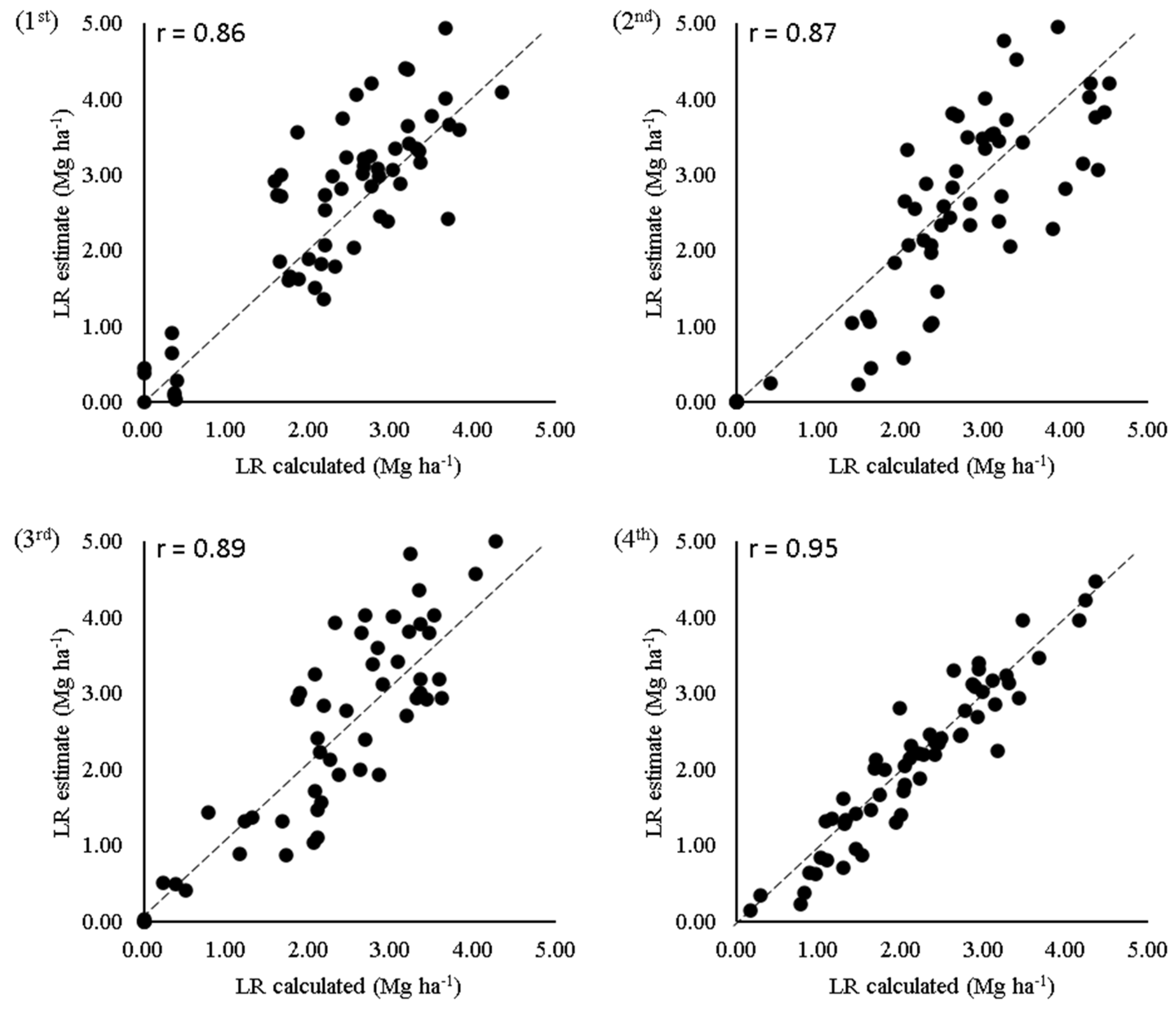
Since both the CEC and BS are necessary to calculate liming recommendations using the BS method [5], the results for R2, RPD, and RPIQ show that it is possible to calculate liming recommendations based on the values estimated by the CEC and BS PLSR models.
Once again, an improvement was noted in most PLSR models with iPLS selection (Table 6) compared to models without iPLS selection (Table A1). After iPLS selection, the R2 values at the calibration stage were on average 4% higher, and in particular, the results for Ca2+ and BS showed increases of 7% and 9%, respectively. There was an average reduction of 18% in the calibration RMSE for models with iPLS for Ca2+, K+, SB, CECe, CEC, and BS compared to the PLSR models without iPLS selection; notable results were seen for Ca2+ and BS, which showed reductions of 39% and 27%, respectively. In the validation phase, there was an average increase of 4% in the R2 values for Ca2+, Mg2+, K+, P, SB, CECe, CEC, and BS, and the values of R2 for Mg2+ and BS increased by 7% and 8%, respectively. Again, in the validation phase, there was an average reduction of 13% in the RMSE for models with iPLS, where the values for Ca2+, K+, and BS showed reductions of 31%, 14%, and 17%, respectively. The results for K+ and BS were notable in the prediction phase, as these showed increases of 13% and 12% in R2 and reductions of 11% and 48% in RMSE, respectively. The prediction results for the RMSE for CEC were also significant, with a reduction of 50%. For Ca2+ and Mg2+, there were increases in RMSE of 15% and 4%, respectively, in the models with iPLS. These results indicate a greater reduction in the RMSE in the models with iPLS, particularly for the CEC and BS, which are characteristics used for liming recommendation in the BS method [5].
In most cases, the reduction in the RMSE values obtained by the PLSR models with iPLS (in the four evaluations) improved the predictive capacity of these models, since the RMSE measures the differences between the estimated values and the real values, and hence quantifies the accuracy of the model. Reductions in the RMSE values therefore gave rise to better accuracy for these models.
Furthermore, for all the characteristics studied for the four soil samples (Table 3, Table 4, Table 5 and Table 6), the systematic error values (BIAS) in the calibration and validation phases were close to zero; these results demonstrate the very low bias of the model in regard to the estimated characteristics [68]. Willmott [69] states that PLSR models are considered to be good when the BIAS approaches zero, similarly to the results in the prediction phase for characteristics with R2 above 0.6 (Table 3, Table 4, Table 5 and Table 6).
Thus, there was a gradual evolution of the statistical parameters from the first to the fourth assessment; this may have been because as the treatments (limestone and phosphogypsum) reacted with the soil over the years, greater amplitudes in the chemical characteristics of the soil were generated, allowing us to find better models.

3.5. Spectral-Based Method for Liming Recommendation

Figure 7 shows the results of a correlation analysis between the estimated liming recommendation using the characteristics obtained by the PLSR models, and the calculated liming recommendation using the characteristics obtained by conventional laboratory techniques. The first soil assessment showed the lowest correlation (r = 0.86), and the correlation values increased up to the fourth soil assessment, for which the correlation coefficient was 0.95. These results therefore show that over the four soil assessments (5, 12, 24, and 36 months after the application of treatments), the liming recommendations based on the chemical characteristics obtained by the PLSR models became progressively more correlated with the liming recommendations calculated based on the chemical characteristics obtained by conventional laboratory techniques. This was probably due to the limestone reaction time. Several studies of Brazilian soils have demonstrated that three years is sufficient for all of the applied limestone to undergo reaction [6,70,71]. Thus, for our very clayey Oxisol, liming recommendations based on multivariate statistical modeling of soil reflectance should preferably be made three years after the last liming, as in this case, the prediction models for CEC and BS had values of R2 for prediction of 0.90 (Table 6).

4. Conclusions

Our models were shown to discriminate between the layers sampled from the soil profile with high accuracy, although models discriminating among treatments could not be developed.
The use of iPLS selection gave rise to an increase in R2 and a reduction in the RMSE values for most PLSR models developed for all four soil assessments, which improved the accuracy of these models.
We were able to estimate the soil chemical characteristics by selecting wavelengths using the iPLS method and PLSR modeling, and, in particular, for Ca2+, SB, CTCe, CTC, and BS. The statistical parameters of these models gradually improved until the fourth assessment. The values of R2 ranged from 0.83 to 0.92 in the calibration and validation steps, and from 0.84 to 0.90 in the prediction step (in the fourth assessment).
The PLSR models of CEC and BS made it possible to calculate a liming recommendation based on the chemical characteristics estimated by the PLSR models. This estimate was positively correlated (r > 0.86) with the liming recommendation calculated based on the chemical characteristics obtained by conventional laboratory techniques. The fourth soil assessment yielded the best correlation coefficient (r = 0.95).
Our results demonstrate that the use of Vis-NIR-SWIR spectroscopy in conjunction with the selection of iPLS variables technique has strong potential in terms of predicting soil chemical characteristics, and can complement conventional analyses of these characteristics. This approach has several advantages, as it has a low cost, does not use toxic reagents, and can be used when many soil samples are required, for example in precision agriculture. In addition, the possibility of using a smaller number of wavelengths to estimate soil chemical characteristics may enable the use of cheaper sensors and automated recommendations for liming tropical soils. However, more work on wavelength selection for PLSR modeling needs to be done.

Author Contributions

Conceptualization, G.L.A.A.d.S., M.R.B., M.A.B. and M.R.N.; methodology, G.L.A.A.d.S., M.R.B., R.H.F., L.G.T.C., M.R., M.A.B. and M.R.N.; software, G.L.A.A.d.S. and R.H.F.; formal analysis, G.L.A.A.d.S., M.R.B., R.H.F., M.R., A.S.R., K.M.d.O. and C.F.C.; data curation, G.L.A.A.d.S., M.R.B., M.A.B. and M.R.N.; writing—original draft preparation, G.L.A.A.d.S.; writing—review and editing, G.L.A.A.d.S., M.R.B., R.H.F., L.G.T.C., M.R., A.S.R., K.M.d.O., C.F.C., R.B.d.O., M.A.B. and M.R.N.; visualization, L.G.T.C., M.R. and R.H.F.; supervision, M.A.B. and M.R.N.; project administration, M.A.B. and M.R.N.; funding acquisition, M.A.B. and M.R.N. All authors have read and agreed to the published version of the manuscript.

Funding

This work was funded by the Coordenação de Aperfeiçoamento de Pessoal de Nível Superior (CAPES PROEX 88882.344501/2019-01), through a doctoral fellowship grant to the first author and resources to carry out the project analyses.

Institutional Review Board Statement

Not applicable.

Informed Consent Statement

Not applicable.

Data Availability Statement

Not applicable.

Acknowledgments

We want to thank COAMO Cooperativa Agroindustrial for allowing this study to be carried out, and particularly João Carlos Bonani, Marcos Vinicios Garbiate, Cristiano Luis Kosinski, and Marcelo Sumiya.

Conflicts of Interest

The authors declare no conflict of interest. The funders had no role in the design of the study; in the collection, analyses, or interpretation of data; in the writing of the manuscript; or in the decision to publish the results.

Appendix A

Table A1. Statistical parameters of the PLSR models developed from the four soil assessments (without iPLS selection).
PLSRCa2+Mg2+K+PS-SO42−pHAl3+H+AlSBCECeCECmBS
cmolc dm−3mg dm−3 cmolc dm−3%
First Assessment
Factors5552136755565
Cal.R20.750.490.760.620.010.420.230.310.770.790.760.310.67
RMSE0.590.370.0620.1527.690.360.150.760.810.740.678.548.98
Val.R20.700.430.740.610.000.400.140.180.720.750.740.210.62
RMSE0.660.400.0620.5428.040.370.160.820.890.800.719.179.68
Pred.R20.730.390.690.600.020.440.140.300.750.770.720.220.65
RMSE0.700.390.0721.3929.610.370.160.800.890.810.7110.439.88
Second Assessment
Factors8559192955625
Cal.R20.780.510.610.720.040.530.050.400.750.780.900.140.62
RMSE0.740.500.139.7619.100.270.220.801.191.050.5610.9111.05
Val.R20.740.460.590.650.030.430.030.260.710.750.880.130.59
RMSE0.820.530.1410.9619.320.300.220.891.271.110.6111.0111.58
Pred.R20.690.320.570.610.050.320.000.160.650.700.860.000.47
RMSE0.780.570.1210.0424.170.310.200.781.241.100.629.4611.91
Third Assessment
Factors610631107867597
Cal.R20.760.680.760.720.000.530.270.270.790.830.800.390.67
RMSE0.770.430.079.1420.670.290.240.921.080.911.0110.279.64
Val.R20.740.580.730.700.000.410.160.120.760.800.780.260.61
RMSE0.820.490.089.5220.870.330.251.011.171.011.0711.3410.51
Pred.R20.710.480.640.720.000.360.130.200.800.840.810.100.64
RMSE0.920.470.098.8111.190.340.241.081.040.880.8611.8910.34
Fourth Assessment
Factors6534210109654106
Cal.R20.860.600.800.820.170.660.530.540.870.880.880.600.79
RMSE0.430.410.086.344.860.210.160.450.660.590.578.156.97
Val.R20.840.550.790.810.150.560.380.400.850.860.870.470.76
RMSE0.470.430.086.674.940.250.180.510.700.640.599.547.48
Pred.R20.820.570.650.730.090.430.100.300.840.860.810.270.79
RMSE0.460.430.108.087.060.280.180.630.700.630.728.787.09
Ca2+, Mg2+, and Al3+ contents were extracted using KCl 1.0 mol L−1; K+ and P contents were extracted using Mehlich-1; pH CaCl2 (0.01 mol L−1) at a soil:solution rate of 1:2.5; H+Al was extracted using the SMP method; CECe: effective cation exchange capacity; CEC: cation exchange capacity at pH 7; m: aluminum saturation; BS: base saturation; R2: coefficient of determination; RMSE: root mean square error.

References

  1. Malavolta, E. Seminário Sobre Corretivos Agrícolas; Fundação Cargil: São Paulo, Brazil, 1985; pp. 313–357. [Google Scholar]
  2. Novais, R.F.; Alvarez, V.H.; de Barros, M.F.; Fontes, R.L.F.; Cantarutti, R.B.; Neves, J.C.L. Fertilidade Do Solo; SBCS: Viçosa, Brazil, 2007. [Google Scholar]
  3. Bayer, C.; Bissani, C.A.; Zanatta, J.A. Química de Solos Em Plantio Direto. In Manejo Da Fertil; De Solos Em Plantio Direto: Guarapuava Fapa, Brazil, 2006; pp. 7–26. [Google Scholar]
  4. Ernane, P.R. Química Do Solo e Disponibilidade de Nutrientes; Ernani, P.R., Ed.; 2008; p. 230. ISBN 8590844005. Available online: https://www.amazon.com.br/Qu%C3%ADmica-do-Solo-Disponibilidade-Nutrientes/dp/8590844005 (accessed on 1 January 2022).
  5. SBCS/NEPAR. Manual de Adubação e Calagem Para o Estado Do Paraná Curitiba; Sociedade Brasileira de Ciência do Solo—Núcleo Estadual Paraná: Estadual Paraná, Brazil, 2017; p. 482. ISBN 978-85-69416-07-0. [Google Scholar]
  6. Sousa, D.M.G.; Lobato, E. Calagem Avaliada Em Plantio Direto Num Latossolo Do Cerrado. Embrapa Cerrados-Fôlder/Folheto/Cart. (INFOTECA-E) 2004. Available online: https://www.infoteca.cnptia.embrapa.br/infoteca/bitstream/doc/567445/1/p200218.pdf (accessed on 1 January 2022).
  7. Caires, E.F. Controle Da Acidez e Melhoria Do Ambiente Radicular No Sistema Plantio Direto. In Fertilidade do Solo e Nutrição de Plantas no Sistema Plantio Direto; Ponta Grossa Assoc& Dos Eng, Agrônomos Dos Campos Gerais/University Estadual De Ponta Grossa: Estadual De Ponta Grossa, Brazil, 2011; pp. 23–68. [Google Scholar]
  8. Lopes, A.S.; Silva, M.C.; Guilherme, L.R.G. Acidez Do Solo e Calagem; ANDA: São Paulo, Brazil, 1990; p. 22. [Google Scholar]
  9. Caires, E.F.; Blum, J.; Barth, G.; Garbuio, F.J.; Kusman, M.T. Alterações Químicas Do Solo e Resposta Da Soja Ao Calcário e Gesso Aplicados Na Implantação Do Sistema Plantio Direto. Rev. Bras. De Ciência Do Solo 2003, 27, 275–286. [Google Scholar] [CrossRef]
  10. Costa, C.H.M.; Castro, G.S.A.; Ferrari Neto, J.; Guimarães, T.M. Gessagem No Sistema Plantio Direto. J. Agron. Sci. 2015, 201–215. [Google Scholar]
  11. Abracal Consumo Aparente Por Estado–Período 1992/2020. Available online: https://abracal.com.br/site/estatisticas/ (accessed on 27 January 2022).
  12. Demattê, J.A.M.; Alves, M.R.; Gallo, B.C.; Fongaro, C.T.; Souza, A.B.E.; Romero, D.J.; Sato, M.V. Hyperspectral Remote Sensing as an Alternative to Estimate Soil Attributes. Rev. Ciência Agronômica 2015, 46, 223–232. [Google Scholar] [CrossRef]
  13. Cherubin, M.R.; Santi, A.L.; Eitelwein, M.T.; Amado, T.J.C.; Simon, D.H.; Damian, J.M. Dimensão Da Malha Amostral Para Caracterização Da Variabilidade Espacial de Fósforo e Potássio Em Latossolo Vermelho. Pesqui. Agropecuária Bras. 2015, 50, 168–177. [Google Scholar] [CrossRef] [Green Version]
  14. Nanni, M.R.; Povh, F.P.; Demattê, J.A.M.; de Oliveira, R.B.; Chicati, M.L.; Cezar, E. Optimum Size in Grid Soil Sampling for Variable Rate Application in Site-Specific Management. Sci. Agric. 2011, 68, 386–392. [Google Scholar] [CrossRef] [Green Version]
  15. Furlanetto, R.H.; Rafael Nanni, M.; Guilherme Teixeira Crusiol, L.; Silva, G.F.C.; Junior, A.D.O.; Sibaldelli, R.N.R. Identification and Quantification of Potassium (K+) Deficiency in Maize Plants Using an Unmanned Aerial Vehicle and Visible/near-Infrared Semi-Professional Digital Camera. Int. J. Remote Sens. 2021, 42, 8783–8804. [Google Scholar] [CrossRef]
  16. Viscarra Rossel, R.A.; Adamchuk, V.I.; Sudduth, K.A.; McKenzie, N.J.; Lobsey, C. Proximal Soil Sensing: An Effective Approach for Soil Measurements in Space and Time. Adv. Agron. 2011, 113, 243–291. [Google Scholar]
  17. Kodaira, M.; Shibusawa, S. Using a Mobile Real-Time Soil Visible-near Infrared Sensor for High Resolution Soil Property Mapping. Geoderma 2013, 199, 64–79. [Google Scholar] [CrossRef]
  18. Viscarra Rossel, R.A.; Jeon, Y.S.; Odeh, I.O.A.; McBratney, A.B. Using a Legacy Soil Sample to Develop a Mid-IR Spectral Library. Soil Res. 2008, 46, 1–16. [Google Scholar] [CrossRef]
  19. Bellon-Maurel, V.; Fernandez-Ahumada, E.; Palagos, B.; Roger, J.-M.; McBratney, A. Critical Review of Chemometric Indicators Commonly Used for Assessing the Quality of the Prediction of Soil Attributes by NIR Spectroscopy. TrAC Trends Anal. Chem. 2010, 29, 1073–1081. [Google Scholar] [CrossRef]
  20. Chabrillat, S.; Ben-Dor, E.; Viscarra Rossel, R.A.; Demattê, J.A.M. Quantitative Soil Spectroscopy. Appl. Environ. Soil Sci. 2013, 2013, 616578. [Google Scholar] [CrossRef]
  21. Das, B.S.; Sarathjith, M.C.; Santra, P.; Sahoo, R.N.; Srivastava, R.; Routray, A.; Ray, S.S. Hyperspectral Remote Sensing: Opportunities, Status and Challenges for Rapid Soil Assessment in India. Curr. Sci. 2015, 108, 860–868. [Google Scholar] [CrossRef]
  22. Zornoza, R.; Guerrero, C.; Mataix-Solera, J.; Scow, K.M.; Arcenegui, V.; Mataix-Beneyto, J. Near Infrared Spectroscopy for Determination of Various Physical, Chemical and Biochemical Properties in Mediterranean Soils. Soil Biol. Biochem. 2008, 40, 1923–1930. [Google Scholar] [CrossRef] [PubMed] [Green Version]
  23. Du, C.; Zhou, J. Evaluation of Soil Fertility Using Infrared Spectroscopy–A Review. Clim. Change Intercropping Pest Control. Benef. Microorg. 2009, 7, 453–483. [Google Scholar]
  24. Tekin, Y.; Kuang, B.; Mouazen, A.M. Potential of On-Line Visible and near Infrared Spectroscopy for Measurement of PH for Deriving Variable Rate Lime Recommendations. Sensors 2013, 13, 10177–10190. [Google Scholar] [CrossRef]
  25. Terra, F.S.; Demattê, J.A.M.; Viscarra Rossel, R.A. Spectral Libraries for Quantitative Analyses of Tropical Brazilian Soils: Comparing Vis–NIR and Mid-IR Reflectance Data. Geoderma 2015, 255–256, 81–93. [Google Scholar] [CrossRef]
  26. Pinheiro, É.; Ceddia, M.; Clingensmith, C.; Grunwald, S.; Vasques, G. Prediction of Soil Physical and Chemical Properties by Visible and Near-Infrared Diffuse Reflectance Spectroscopy in the Central Amazon. Remote Sens. 2017, 9, 293. [Google Scholar] [CrossRef] [Green Version]
  27. Bai, L.; Wang, C.; Zang, S.; Wu, C.; Luo, J.; Wu, Y. Mapping Soil Alkalinity and Salinity in Northern Songnen Plain, China with the HJ-1 Hyperspectral Imager Data and Partial Least Squares Regression. Sensors 2018, 18, 3855. [Google Scholar] [CrossRef] [Green Version]
  28. Rodrigues, M.; Nanni, M.R.; Cezar, E.; Abrantes dos Santos, G.L.A.; Silveira Reis, A.; de Oliveira, K.M. Evaluation of the Use of Spectroradiometry for the Determination of Soil Exchangeable Ions after the Application of Mining Coproducts. Appl. Spectrosc. Rev. 2020, 55, 491–508. [Google Scholar] [CrossRef]
  29. Ben-Dor, E.; Banin, A. Near-infrared Analysis as a Rapid Method to Simultaneously Evaluate Several Soil Properties. Soil Sci. Soc. Am. J. 1995, 59, 364–372. [Google Scholar] [CrossRef]
  30. Ben-Dor, E.; Chabrillat, S.; Demattê, J.A.M.; Taylor, G.R.; Hill, J.; Whiting, M.L.; Sommer, S. Using Imaging Spectroscopy to Study Soil Properties. Remote Sens. Environ. 2009, 113, S38–S55. [Google Scholar] [CrossRef]
  31. Janik, L.J.; Merry, R.H.; Skjemstad, J.O. Can Mid Infrared Diffuse Reflectance Analysis Replace Soil Extractions? Aust. J. Exp. Agric. 1998, 38, 681. [Google Scholar] [CrossRef]
  32. Reeves, J.B.; McCarty, G.W.; Meisinger, J.J. Near Infrared Reflectance Spectroscopy for the Analysis of Agricultural Soils. J. Near Infrared Spectrosc. 1999, 7, 179–193. [Google Scholar] [CrossRef]
  33. Nanni, M.R.; Cezar, E.; da Silva Junior, C.A.; Silva, G.F.C.; da Silva Gualberto, A.A. Partial Least Squares Regression (PLSR) Associated with Spectral Response to Predict Soil Attributes in Transitional Lithologies. Arch. Agron. Soil Sci. 2018, 64, 682–695. [Google Scholar] [CrossRef]
  34. Viscarra Rossel, R.A.; Walvoort, D.J.J.; McBratney, A.B.; Janik, L.J.; Skjemstad, J.O. Visible, near Infrared, Mid Infrared or Combined Diffuse Reflectance Spectroscopy for Simultaneous Assessment of Various Soil Properties. Geoderma 2006, 131, 59–75. [Google Scholar] [CrossRef]
  35. Li, H.; Liang, Y.; Xu, Q.; Cao, D. Key Wavelengths Screening Using Competitive Adaptive Reweighted Sampling Method for Multivariate Calibration. Anal. Chim. Acta 2009, 648, 77–84. [Google Scholar] [CrossRef]
  36. Xiaobo, Z.; Jiewen, Z.; Povey, M.J.W.; Holmes, M.; Hanpin, M. Variables Selection Methods in Near-Infrared Spectroscopy. Anal. Chim. Acta 2010, 667, 14–32. [Google Scholar] [CrossRef]
  37. Vohland, M.; Ludwig, M.; Thiele-Bruhn, S.; Ludwig, B. Determination of Soil Properties with Visible to Near-and Mid-Infrared Spectroscopy: Effects of Spectral Variable Selection. Geoderma 2014, 223, 88–96. [Google Scholar] [CrossRef]
  38. Sarathjith, M.C.; Das, B.S.; Wani, S.P.; Sahrawat, K.L. Variable Indicators for Optimum Wavelength Selection in Diffuse Reflectance Spectroscopy of Soils. Geoderma 2016, 267, 1–9. [Google Scholar] [CrossRef]
  39. Wise, B.M.; Gallagher, N.B.; Bro, R.; Shaver, J.; Windig, W.; Koch, R.S. PLS Toolbox 4.0. 2007. Available online: http://mitr.p.lodz.pl/raman/jsurmacki/pliki/zajecia/LMDiT/cw3/LMDiT_PLS_Manual_4.pdf (accessed on 1 January 2022).
  40. Nørgaard, L.; Saudland, A.; Wagner, J.; Nielsen, J.P.; Munck, L.; Engelsen, S.B. Interval Partial Least-Squares Regression (iPLS): A Comparative Chemometric Study with an Example from Near-Infrared Spectroscopy. Appl. Spectrosc. 2000, 54, 413–419. [Google Scholar] [CrossRef]
  41. Andersen, C.M.; Bro, R. Variable Selection in Regression—A Tutorial. J. Chemom. 2010, 24, 728–737. [Google Scholar] [CrossRef]
  42. Caviglione, J.H.; Kiihl, L.R.B.; Caramori, P.H.; Oliveira, D.; Galdino, J.; Borrozino, E.; Pugsley, L. Cartas Climáticas do Estado do Paraná [CD-ROM]. In Proceedings of the Congresso E Mostra De Agroinformática, Ponta Grossa, Paraná, Brazil, 18–20 October 2000. [Google Scholar]
  43. Santos, H.G.; Jacomine, P.K.T.; Dos Anjos, L.H.C.; De Oliveira, V.A.; Lumbreras, J.F.; Coelho, M.R.; De Almeida, J.A.; de Araujo Filho, J.C.; Oliveira, J.B.; Cunha, T.J.F. Sistema Brasileiro de Classificação de Solos; Embrapa: Brasília, Brazil, 2018; ISBN 8570358172. [Google Scholar]
  44. WRB. International Soil Classification System for Naming Soils and Creating Legends for Soil Maps; Fao Rome: Rome, Italy, 2015. [Google Scholar]
  45. Staff, S.S. Soil Taxonomy: A Basic System of Soil Classification for Making and Interpreting Soil Surveys. In Agriculture Handbook; Routledge: London, UK, 1999; Volume 436. [Google Scholar]
  46. Souza, D.M.G.; Lobato, E.; Rein, T.A. Uso Do Gesso Agrícola Nos Solos Dos Cerrados. Planaltina Embrapa Cerrados 2005, 19. [Google Scholar]
  47. Pavan, M.A.; Bloch, M.D.F.; Zempulski, H.D.C.; Miyazawa, M.; Zocoler, D.C. Manual de Análise Química de Solo e Controle de Qualidade; IAPAR: Londrina, Brazil, 1992; Volume 76. [Google Scholar]
  48. Silva, F.C.D.A.S. Manual de Análises Químicas de Solos, Plantas e Fertilizantes, 2nd ed.; Embrapa Informação Tecnológica; Embrapa Solos Brasília: Rio de Janeiro, Brazil, 2009; Volume 2. [Google Scholar]
  49. Demattê, J.A.M.; Toledo, A.M.A.; Simões, M.S. Metodologia Para Reconhecimento de Três Solos Por Sensores: Laboratorial e Orbital. Rev. Bras. De Ciência Do Solo 2004, 28, 877–889. [Google Scholar] [CrossRef] [Green Version]
  50. Nanni, M.R.; Demattê, J.A.M.; Rodrigues, M.; dos Santos, G.L.A.A.; Reis, A.S.; de Oliveira, K.M.; Cezar, E.; Furlanetto, R.H.; Crusiol, L.G.T.; Sun, L. Mapping Particle Size and Soil Organic Matter in Tropical Soil Based on Hyperspectral Imaging and Non-Imaging Sensors. Remote Sens. 2021, 13, 1782. [Google Scholar] [CrossRef]
  51. Nanni, M.R.; Demattê, J.A.M. Comportamento Da Linha Do Solo Obtida Por Espectrorradiometria Laboratorial Para Diferentes Classes de Solo. Rev. Bras. De Ciência Do Solo 2006, 30, 1031–1038. [Google Scholar] [CrossRef]
  52. Nicodemus, F.E.; Richmond, J.C.; Hsia, J.J.; Ginsberg, I.W.; Limperis, T. Geometrical Considerations and Nomenclature for Reflectance. NBS Monogr. 1992, 160, 4. [Google Scholar]
  53. Savitzky, A.; Golay, M.J.E. Smoothing and Differentiation of Data by Simplified Least Squares Procedures. Anal. Chem. 1964, 36, 1627–1639. [Google Scholar] [CrossRef]
  54. Jahani, S.; Setarehdan, S.K.; Boas, D.A.; Yücel, M.A. Motion Artifact Detection and Correction in Functional Near-Infrared Spectroscopy: A New Hybrid Method Based on Spline Interpolation Method and Savitzky–Golay Filtering. Neurophotonics 2018, 5, 015003. [Google Scholar] [CrossRef] [Green Version]
  55. Karimi, Y.; Prasher, S.O.; McNairn, H.; Bonnell, R.B.; Dutilleul, P.; Goel, P.K. Classification Accuracy of Discriminant Analysis, Artificial Neural Networks, and Decision Trees for Weed and Nitrogen Stress Detection in Corn. Trans. ASAE 2005, 48, 1261–1268. [Google Scholar] [CrossRef]
  56. Nanni, M.R.; Demattê, J.A.M.; Fiorio, P.R. Análise Discriminante Dos Solos Por Meio Da Resposta Espectral No Nível Terrestre. Pesqui. Agropecuária Bras. 2004, 39, 995–1006. [Google Scholar] [CrossRef] [Green Version]
  57. Cezar, E.; Nanni, M.R.; Demattê, J.A.M.; Chicati, M.L.; de Oliveira, R.B. Estimativa de Atributos Do Solo Por Meio de Espectrorradiometria Difusa. Rev. Bras. De Ciência Do Solo 2013, 37, 858–868. [Google Scholar] [CrossRef] [Green Version]
  58. Wise, B.M.; Gallagher, N.B.; Bro, R.; Shaver, J.M.; Windig, W.; Koch, R.S. Chemometrics Tutorial for PLS_Toolbox and Solo. Eig. Res. Inc. 2006, 3905, 102–159. [Google Scholar]
  59. Höskuldsson, A. PLS Regression Methods. J. Chemom. 1988, 2, 211–228. [Google Scholar] [CrossRef]
  60. Wenjun, J.; Zhou, S.; Jingyi, H.; Shuo, L. In Situ Measurement of Some Soil Properties in Paddy Soil Using Visible and Near-Infrared Spectroscopy. PLoS ONE 2014, 9, e105708. [Google Scholar] [CrossRef] [Green Version]
  61. Williams, P.; Manley, M.; Antoniszyn, J. Near Infrared Technology: Getting the Best out of Light; African Sun Media: Stellenbosch, South Africa, 2019; ISBN 1928480306. [Google Scholar]
  62. Saeys, W.; Mouazen, A.M.; Ramon, H. Potential for Onsite and Online Analysis of Pig Manure Using Visible and Near Infrared Reflectance Spectroscopy. Biosyst. Eng. 2005, 91, 393–402. [Google Scholar] [CrossRef]
  63. Chang, C.-W.; Laird, D.A.; Mausbach, M.J.; Hurburgh, C.R. Near-Infrared Reflectance Spectroscopy-Principal Components Regression Analyses of Soil Properties. Soil Sci. Soc. Am. J. 2001, 65, 480–490. [Google Scholar] [CrossRef] [Green Version]
  64. Ludwig, B.; Vormstein, S.; Niebuhr, J.; Heinze, S.; Marschner, B.; Vohland, M. Estimation Accuracies of near Infrared Spectroscopy for General Soil Properties and Enzyme Activities for Two Forest Sites along Three Transects. Geoderma 2017, 288, 37–46. [Google Scholar] [CrossRef]
  65. Abdelmalik, K.W. Landsat 8: Utilizing Sensitive Response Bands Concept for Image Processing and Mapping of Basalts. Egypt. J. Remote Sens. Space Sci. 2020, 23, 263–274. [Google Scholar] [CrossRef]
  66. Veum, K.S.; Sudduth, K.A.; Kremer, R.J.; Kitchen, N.R. Estimating a Soil Quality Index with VNIR Reflectance Spectroscopy. Soil Sci. Soc. Am. J. 2015, 79, 637–649. [Google Scholar] [CrossRef]
  67. Cezar, E.; Nanni, M.R.; Guerrero, C.; da Silva Junior, C.A.; Cruciol, L.G.T.; Chicati, M.L.; Silva, G.F.C. Organic Matter and Sand Estimates by Spectroradiometry: Strategies for the Development of Models with Applicability at a Local Scale. Geoderma 2019, 340, 224–233. [Google Scholar] [CrossRef]
  68. Mark, H.; Workman, J., Jr. Bias and Slope Correction. Spectroscopy 2017, 32, 24–30. [Google Scholar]
  69. Willmott, C.J. Some Comments on the Evaluation of Model Performance. Bull. Am. Meteorol. Soc. 1982, 63, 1309–1313. [Google Scholar] [CrossRef] [Green Version]
  70. Quaggio, J.A.; Mascarenhas, H.A.A.; Bataglia, O.C. Resposta Da Soja à Aplicação de Doses Crescentes de Calcário Em Latossolo Roxo Distrófico de Cerrado, II. Efeito Residual [Soybean response to application of crescent rates of liming on Cerrado dystrophic dusky-red latosol. II. Residual effect]. Rev. Bras. De Cienc. Do Solo 1982, 6, 113–118. [Google Scholar]
  71. De Sousa, D.M.G.; Lobato, E. Cerrado: Correção Do Solo e Adubação.[Cerrado: Soil Correction and Fertilization]; Embrapa Cerrados: Planaltina, Brazil, 2004; p. 416. [Google Scholar]
Figure 1. Location of the experimental area in the municipality of Campo Mourão, State of Paraná, Brazil.
Remotesensing 14 01972 g001
Figure 2. Minimum and maximum temperatures (°C) and precipitation (mm) for the experimental area (June 2016 to May 2019).
Remotesensing 14 01972 g002
Figure 3. Experimental setup used to obtain spectral data from soil samples.
Remotesensing 14 01972 g003
Figure 4. Accuracy of the discriminant models for calibration and validation of the four soil assessments (1st = first assessment; 2nd = second assessment; 3rd = third assessment; 4th = fourth assessment) of six different layers (A = 0.00–0.05 m, B = 0.05–0.10 m, C = 0.10–0.20 m, D = 0.20–0.30 m, E = 0.30–0.40 m, F = 0.40–0.60 m).
Remotesensing 14 01972 g004
Figure 5. Example of selection of iPLS variables for CEC in the second soil assessment. The Y-axis unit is in reflectance factor for the mean sample, and for RMSECV is in cmolc dm−3.
Remotesensing 14 01972 g005
Figure 6. Wavelengths selected by the iPLS method for each variable in the four soil assessments: (a) Ca2+, (b) Mg2+, (c) K+, (d) P, (e) S-SO4−2, (f) pH, (g) Al3+, (h) H+Al, (i) SB, (j) CECe, (k) CEC, (l) m%, and (m) BS.
Remotesensing 14 01972 g006
Figure 7. Correlations between the calculated liming recommendation (LR) (based on chemical characteristics obtained by conventional laboratory techniques) and the liming recommendation (LR) estimated using PLSR models (based on the chemical characteristics obtained by the PLSR models) for four soil assessments (1st = first assessment; 2nd = second assessment; 3rd = third assessment; 4th = fourth assessment).
Remotesensing 14 01972 g007
Table 1. Chemical characterization of the soil before treatment in 2016 and limestone application rates used.
TreatmentLayerCa2+Mg2+K+PpHH+AlCECmBSLime Rate
mcmolc dm−3mg dm−3CaCl2cmolc dm−3%Mg ha−1
IL BS% 440.00–0.202.860.580.3922.814.975.359.182.0541.72-
0.20–0.402.040.390.287.914.755.968.674.9131.26-
IL BS% 600.00–0.202.730.630.2323.554.795.559.144.0139.282.3
0.20–0.402.140.510.207.144.825.158.004.0435.63-
IL BS% 700.00–0.203.240.880.2921.375.084.619.020.0048.892.3
0.20–0.402.780.700.2510.265.234.448.170.0045.65-
IL BS% 900.00–0.203.030.990.3020.885.075.559.870.0043.775.6
0.20–0.402.300.740.257.804.844.968.252.9539.88-
SL BS% 440.00–0.203.520.740.2621.385.005.159.670.8846.74-
0.20–0.402.120.410.205.084.745.157.886.5134.64-
SL BS% 600.00–0.203.470.90.2630.065.164.969.590.0048.281.4
0.20–0.402.140.560.198.024.924.787.672.6937.68-
SL BS% 700.00–0.203.111.000.2413.735.244.288.630.0050.412.1
0.20–0.402.550.770.226.125.144.447.980.0044.36-
SL BS% 900.00–0.203.571.460.2122.445.414.289.520.0055.044.1
0.20–0.402.040.730.188.674.805.158.14.8436.42-
BS60+G50 *0.00–0.204.110.860.2623.185.294.289.510.0054.990.6
0.20–0.402.400.450.205.684.974.617.660.9739.82-
BS70+G50 *0.00–0.203.090.700.1926.745.004.618.590.7546.332.5
0.20–0.401.710.340.155.394.605.357.550.1229.14-
BS70+G100 **0.00–0.203.160.650.1934.345.064.968.960.0044.642.8
0.20–0.402.010.310.147.144.755.357.818.2131.50-
* represents an application rate of 3.71 and ** represents an application rate of 7.42 Mg ha−1 phosphogypsum (G) applied in 2016. The phosphogypsum rate (GR) was calculated as a function of the clay soil content according to the formula GR = 50 × clay (%), as proposed by Sousa et al. [47]. The highest GR application rate was determined based on twice the recommended application rate [GR = 100 × clay (%)]. IL indicates incorporated liming; SL indicates surface liming; G indicates phosphogypsum; Ca2+, Mg2+ and Al3+ contents were extracted using KCl 1.0 mol L−1; K+ and P contents were extracted using Mehlich-1; pH CaCl2 (0.01 mol L−1) at a soil:solution ratio of 1:2.5; H+Al was extracted using the SMP method; CEC is the cation exchange capacity at pH 7 (CEC = Ca2+ + Mg2+ + K+ + H+Al); m represents the aluminum saturation [m=(Al3+/Ca2++Mg2++K++Al3+) × 100]; BS is the base saturation [BS = (Ca2+ + Mg2+ + K+/CEC)].
Table 2. Descriptive analysis of the chemical characteristics of the soil over the four soil assessments.
Statistics *Ca2+Mg2+K+PS-SO42−pHAl3+H+AlSBCECeCECmBS
cmolc dm−3mg dm−3CaCl2cmolc dm−3%
First assessment (five months)
Minimum0.230.140.060.641.653.530.002.540.560.945.040.006.93
Maximum6.803.220.61133.31168.466.580.917.768.598.6111.7758.4275.65
Mean1.770.730.2228.6917.645.080.184.752.722.907.479.7934.21
Std. dev.1.230.520.1233.2428.390.490.170.921.721.631.3710.7215.92
CV %69.3871.7557.57115.87160.899.5693.8919.3963.4956.3418.32109.5146.54
Second assessment (12 months)
Minimum0.310.170.010.250.004.320.062.540.641.255.180.738.36
Maximum7.933.400.87101.40112.806.091.257.1510.0010.1012.7466.2278.80
Mean2.310.840.2315.0821.484.990.284.773.373.658.1411.6938.19
Std. dev.1.560.710.2017.8921.040.390.220.992.302.181.7611.2217.62
CV %67.4984.9790.26118.6897.967.8678.4420.7968.2259.8721.6495.9146.15
Third assessment (24 months)
Minimum0.360.130.050.361.534.220.022.860.641.405.330.238.35
Maximum8.593.390.71107.42258.186.211.5610.0711.4911.6313.5270.8678.20
Mean2.290.850.2316.6419.674.970.335.103.373.708.4713.6836.54
Std. dev.1.630.750.1517.1618.790.430.271.112.382.252.2113.0317.00
CV %71.1787.8065.16103.1195.548.6081.8721.8570.6060.6726.0795.2346.52
Fourth assessment (36 months)
Minimum0.190.120.020.763.704.320.042.600.571.274.460.519.58
Maximum5.463.540.7777.9038.536.101.227.158.568.6412.2068.1575.08
Mean1.810.820.2213.8310.224.940.304.082.863.166.9513.5238.21
Std. dev.1.140.650.1715.225.930.370.220.691.811.691.6512.3815.38
CV %62.8278.2376.93110.0458.027.4475.0016.8363.2253.4623.6991.5840.24
* The data follow the normal Kolmogorov–Smirnov distribution (p-value ≤ 0.01). Ca2+, Mg2+ and Al3+ contents were extracted using KCl 1.0 mol L−1; K+ and P contents were extracted using Mehlich-1; pH CaCl2 (0.01 mol L−1) with a soil:solution ratio of 1:2.5; H+Al was extracted using the SMP method; CECe is the effective cation exchange capacity; CEC is the cation exchange capacity at pH 7; m is the aluminum saturation; BS is the base saturation; CV is the coefficient of variance; std. dev. is the standard deviation.
Table 3. Statistical parameters of PLSR models developed from the first soil assessment (with iPLS selection).
PLSRCa2+Mg2+K+PS-SO42−pHAl3+H+AlSBCECeCECmBS
cmolc dm−3mg dm−3 cmolc dm−3%
Variables109138153679823225126961327113663
Factors5733143355354
CalibrationR20.760.580.760.740.000.590.100.180.810.860.840.260.70
RMSE0.550.350.0515.1628.240.300.160.820.700.630.549.198.40
BIAS0.000.000.000.000.000.000.000.000.000.000.000.000.00
RPD2.041.542.041.961.001.561.051.102.292.712.501.161.83
RPIQ2.581.681.922.760.352.091.361.302.973.194.041.442.52
ValidationR20.740.510.750.730.000.560.070.140.790.840.830.190.68
RMSE0.570.380.0615.6228.720.320.170.850.730.680.569.678.71
BIAS0.060.000.00−0.01−0.070.000.000.000.000.000.000.01−0.02
RPD1.961.432.001.921.001.511.041.082.182.512.431.111.77
RPIQ2.491.541.602.680.351.961.281.262.852.963.891.372.43
PredictionR20.750.000.810.820.000.530.010.270.720.810.730.300.63
RMSE0.710.740.0614.0128.520.300.180.811.040.610.668.9710.37
BIAS0.360.580.012.02−3.45−0.020.060.020.23−0.030.45−1.115.84
RPD2.001.002.292.361.001.461.011.171.892.801.921.201.64
RPIQ2.000.791.602.980.352.091.211.322.003.303.301.472.04
Ca2+, Mg2+, and Al3+ contents were extracted using KCl 1.0 mol L−1; K+ and P contents were extracted using Mehlich-1; pH CaCl2 (0.01 mol L−1) at a soil:solution ratio of 1:2.5; H+Al was extracted using the SMP method; CECe is the effective cation exchange capacity; CEC is the cation exchange capacity at pH 7; m indicates the aluminum saturation; BS is the base saturation; R2 is the coefficient of determination; RMSE is the root mean square error; BIAS is the systematic error; RPD represents the relative percentage deviation; RPIQ is the ratio of performance to interquartile range.
Table 4. Statistical parameters of PLSR models developed from the second soil assessment (with iPLS selection).
PLSRCa2+Mg2+K+PS-SO42−pHAl3+H+AlSBCECeCECmBS
cmolc dm−3mg dm−3 cmolc dm−3%
Variables136181172168362202371751241309382170
Factors9565194966317
CalibrationR20.840.650.740.760.070.620.110.480.860.850.900.230.76
RMSE0.590.420.108.1418.760.230.200.690.830.770.469.778.57
BIAS0.000.000.000.000.000.000.000.000.000.000.000.000.00
RPD2.501.691.962.041.041.621.061.392.672.583.161.142.04
RPIQ3.091.671.992.740.692.221.291.883.293.555.421.532.73
ValidationR20.800.620.730.740.060.540.050.380.840.840.900.160.72
RMSE0.650.430.118.5918.960.260.210.760.870.820.4710.239.15
BIAS0.000.000.000.000.010.000.000.000.000.000.00−0.030.02
RPD2.241.621.921.961.031.471.031.272.502.503.161.091.89
RPIQ2.801.631.812.590.681.961.231.713.143.345.301.462.55
PredictionR20.810.470.700.670.090.200.000.000.850.860.910.030.72
RMSE0.680.530.108.9123.860.360.231.260.900.810.5111.199.45
BIAS0.12−0.03−0.031.51−1.49−0.12−0.07−0.89−0.170.220.283.07−0.01
RPD2.291.371.831.741.051.121.001.002.582.673.331.021.89
RPIQ2.681.331.992.500.541.421.121.033.033.384.881.332.47
Ca2+, Mg2+, and Al3+ contents were extracted using KCl 1.0 mol L−1; K+ and P contents were extracted using Mehlich-1; pH CaCl2 (0.01 mol L−1) at a soil:solution ratio of 1:2.5; H+Al was extracted using the SMP method; CECe is the effective cation exchange capacity; CEC is the cation exchange capacity at pH 7; m represents the aluminum saturation; BS is the base saturation; R2 is the coefficient of determination; RMSE is the root mean square error; BIAS is the systematic error; RPD is the relative percentage deviation; and RPIQ is the ratio of performance to interquartile range.
Table 5. Statistical parameters of PLSR models developed from the third soil assessment (with iPLS selection).
PLSRCa2+Mg2+K+PS-SO42−pHAl3+H+AlSBCECeCECmBS
cmolc dm−3mg dm−3 cmolc dm−3%
Variables8161882418324124482586535
Factors810547108278484
CalibrationR20.820.730.780.770.180.740.360.050.860.860.870.390.67
RMSE0.650.400.078.0118.810.230.211.130.890.840.7310.099.64
BIAS0.000.000.000.000.000.000.000.000.000.000.000.000.00
RPD2.361.922.132.091.101.961.251.032.672.672.771.281.74
RPIQ3.142.022.852.940.482.891.611.033.673.634.241.602.71
ValidationR20.810.690.750.770.090.700.290.030.840.820.860.320.65
RMSE0.680.430.078.3519.900.250.221.150.930.950.7510.749.95
BIAS0.000.000.000.050.000.000.000.000.010.010.00−0.03−0.02
RPD2.291.802.002.091.051.831.191.022.502.362.671.211.69
RPIQ3.001.872.852.820.462.661.531.013.513.214.131.502.62
PredictionR20.710.000.760.280.000.000.000.000.770.870.800.180.66
RMSE0.980.850.0711.11108.204.990.770.961.080.760.8511.8010.06
BIAS0.53−0.660.01−7.50104.704.96−0.730.120.02−0.030.18−0.091.16
RPD1.861.002.041.181.001.001.001.002.092.772.241.101.71
RPIQ2.080.952.852.120.080.130.441.213.024.013.651.362.59
Ca2+, Mg2+, and Al3+ contents were extracted using KCl 1.0 mol L−1; K+ and P contents were extracted using Mehlich-1; pH CaCl2 (0.01 mol L−1) at a soil:solution ratio of 1:2.5; H+Al was extracted using the SMP method; CECe is the effective cation exchange capacity; CEC is the cation exchange capacity at pH 7; m represents the aluminum saturation; BS is the base saturation; R2 is the coefficient of determination; RMSE is the root mean square error; BIAS is the systematic error; RPD is the relative percentage deviation; and RPIQ is the ratio of performance to interquartile range.
Table 6. Statistical parameters of the PLSR models developed from the fourth soil assessment (with iPLS selection).
PLSRCa2+Mg2+K+PS-SO42−pHAl3+H+AlSBCECeCECmBS
cmolc dm−3mg dm−3 cmolc dm−3%
Variables134819564811371261019011723114647
Factors10534310910775610
CalibrationR20.920.630.840.840.160.750.490.670.880.890.910.470.87
RMSE0.310.420.076.515.110.180.160.370.620.560.509.275.47
BIAS0.000.000.000.000.000.000.000.000.000.000.000.000.00
RPD3.541.642.502.501.092.001.401.742.893.023.331.372.77
RPIQ4.052.142.853.470.902.502.112.274.284.234.961.754.34
ValidationR20.890.590.830.820.120.680.380.590.870.870.890.370.83
RMSE0.360.440.076.825.280.210.170.420.650.610.569.016.38
BIAS0.000.000.000.00−0.010.000.000.000.01−0.01−0.05−0.180.04
RPD3.021.562.432.361.071.771.271.562.772.773.021.262.43
RPIQ3.492.052.853.310.882.141.992.004.083.884.431.803.72
PredictionR20.840.010.750.580.190.000.000.000.860.890.900.000.90
RMSE0.540.450.097.906.183.150.361.660.640.840.4815.424.79
BIAS0.840.300.013.961.06−3.14−0.081.480.08−0.490.17−12.64−0.12
RPD2.501.012.001.541.111.001.001.002.673.023.161.003.16
RPIQ2.332.02.222.860.750.140.940.514.152.825.171.054.96
Ca2+, Mg2+, and Al3+ contents were extracted using KCl 1.0 mol L−1; K+ and P contents were extracted using Mehlich-1; pH CaCl2 (0.01 mol L−1) at a soil:solution ratio of 1:2.5; H+Al was extracted using the SMP method; CECe is the effective cation exchange capacity; CEC is the cation exchange capacity at pH 7; m represents the aluminum saturation; BS is the base saturation; R2 is the coefficient of determination; RMSE is the root mean square error; BIAS is the systematic error; RPD is the relative percentage deviation; and RPIQ is the ratio of performance to interquartile range.
Publisher’s Note: MDPI stays neutral with regard to jurisdictional claims in published maps and institutional affiliations.

