
Multi-View Structural Feature Extraction for Hyperspectral Image Classification

Abstract
:1. Introduction
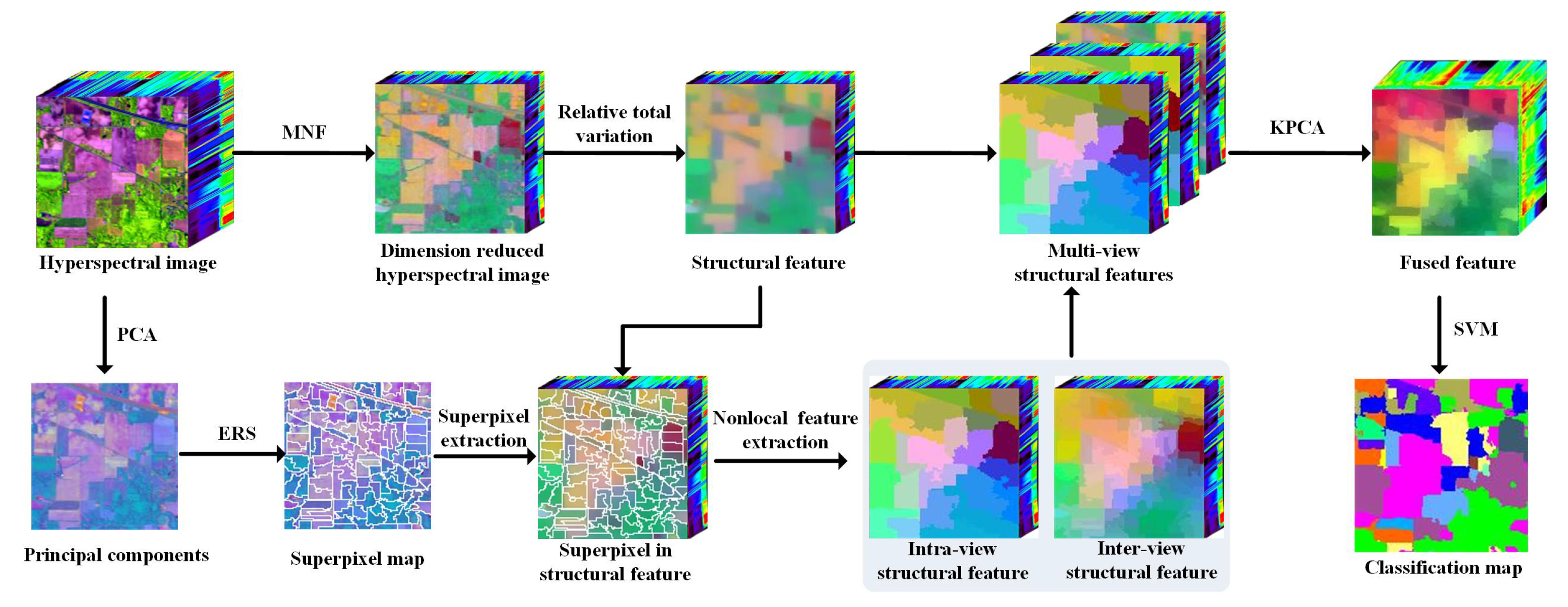
2. Method
2.1. Dimension Reduction
2.2. Multi-View Feature Generation
2.3. Feature Fusion
| Algorithm 1 Multi-view structural feature extraction |
| Input: Input hyperspectral image I; Output: Hyperspectral image feature
|
3. Experiments
3.1. Experimental Setup
3.2. Classification Results
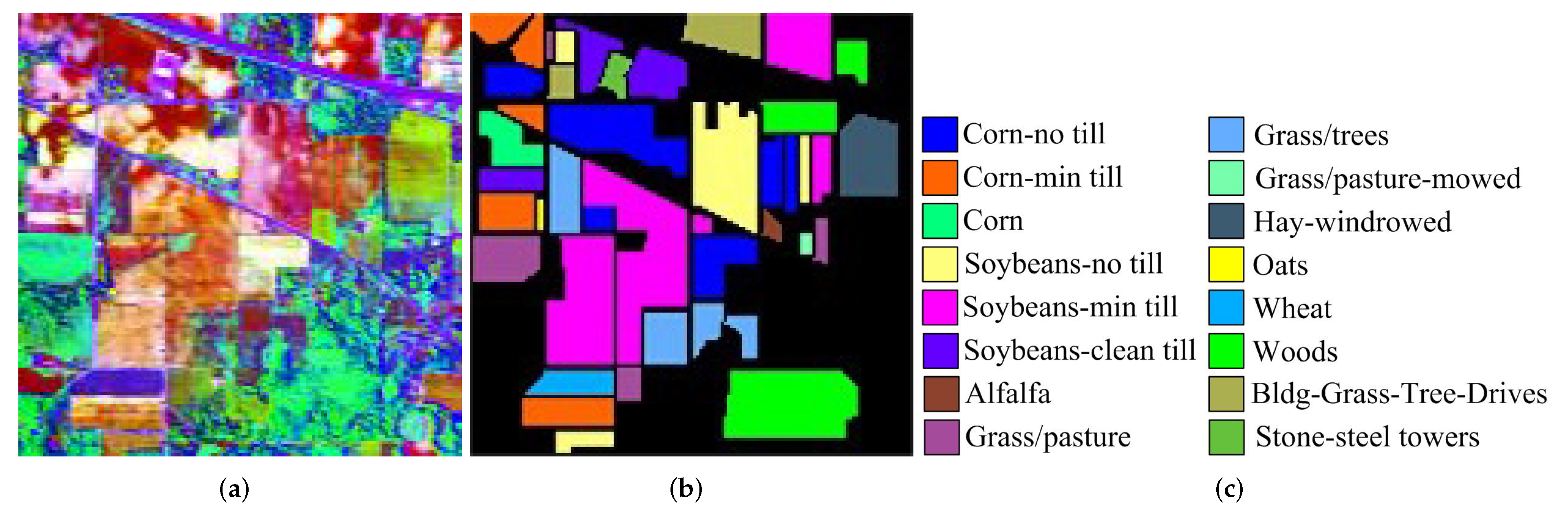
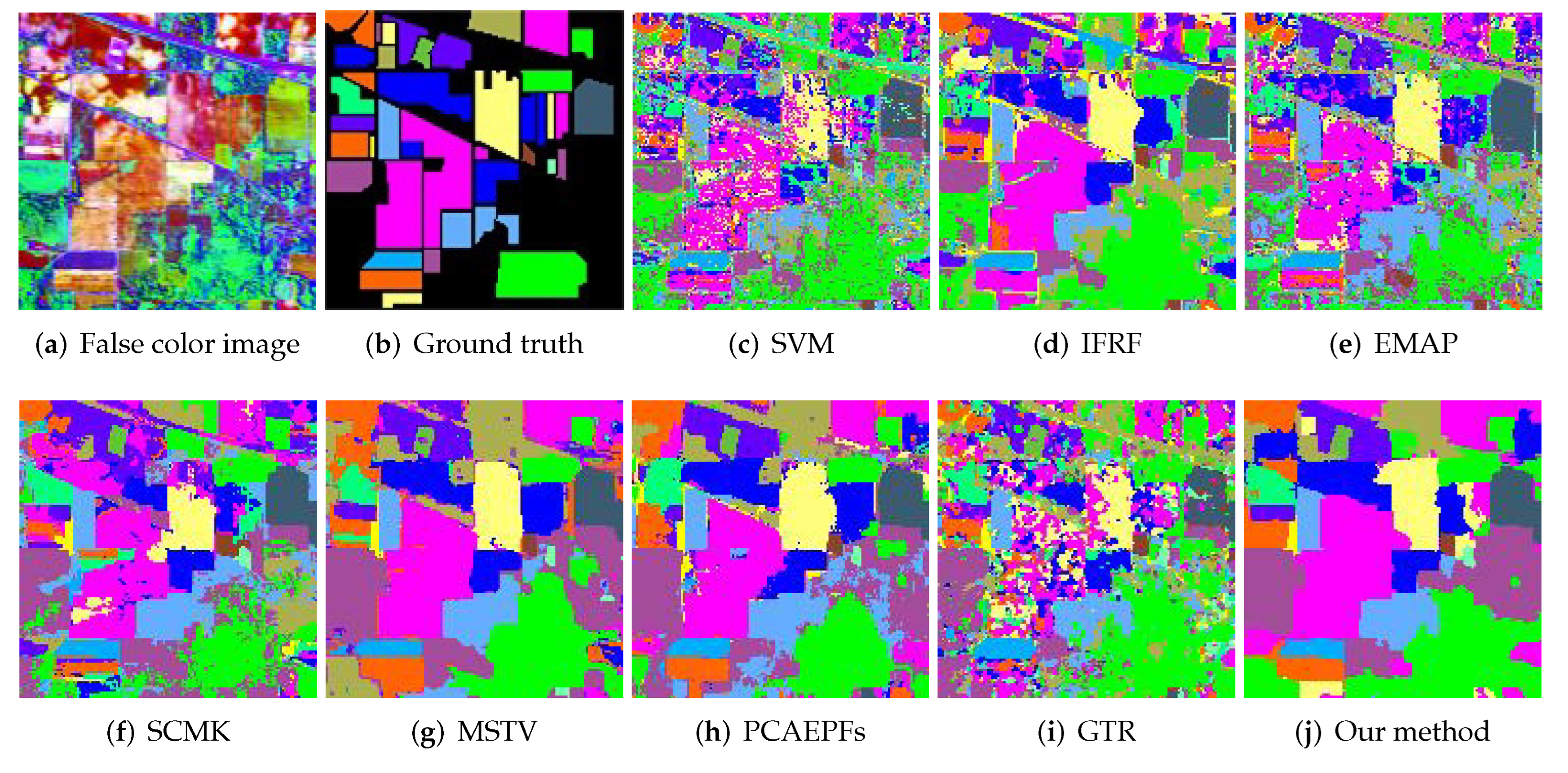
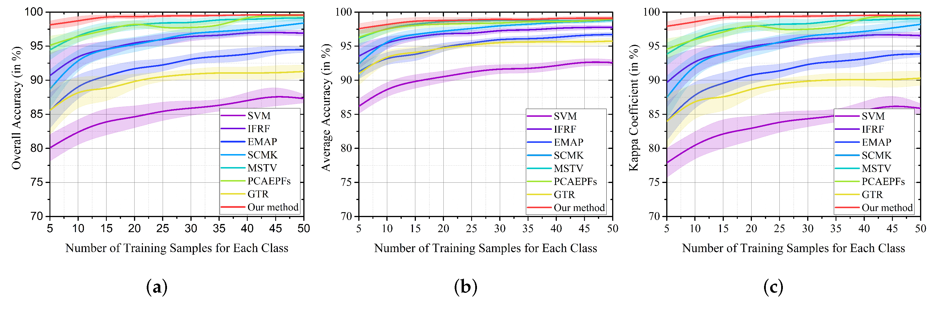
3.2.1. Indian Pines Dataset
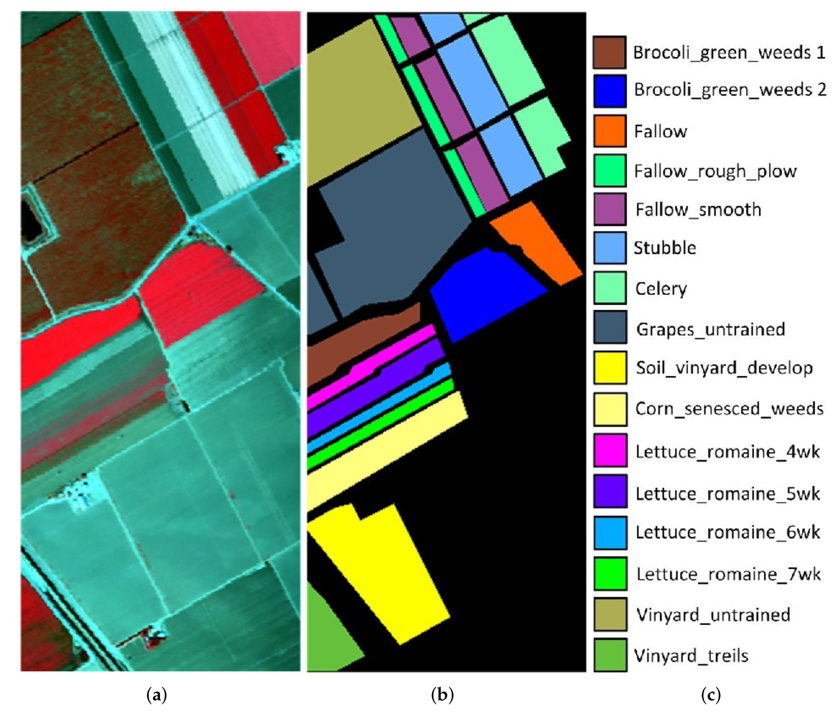
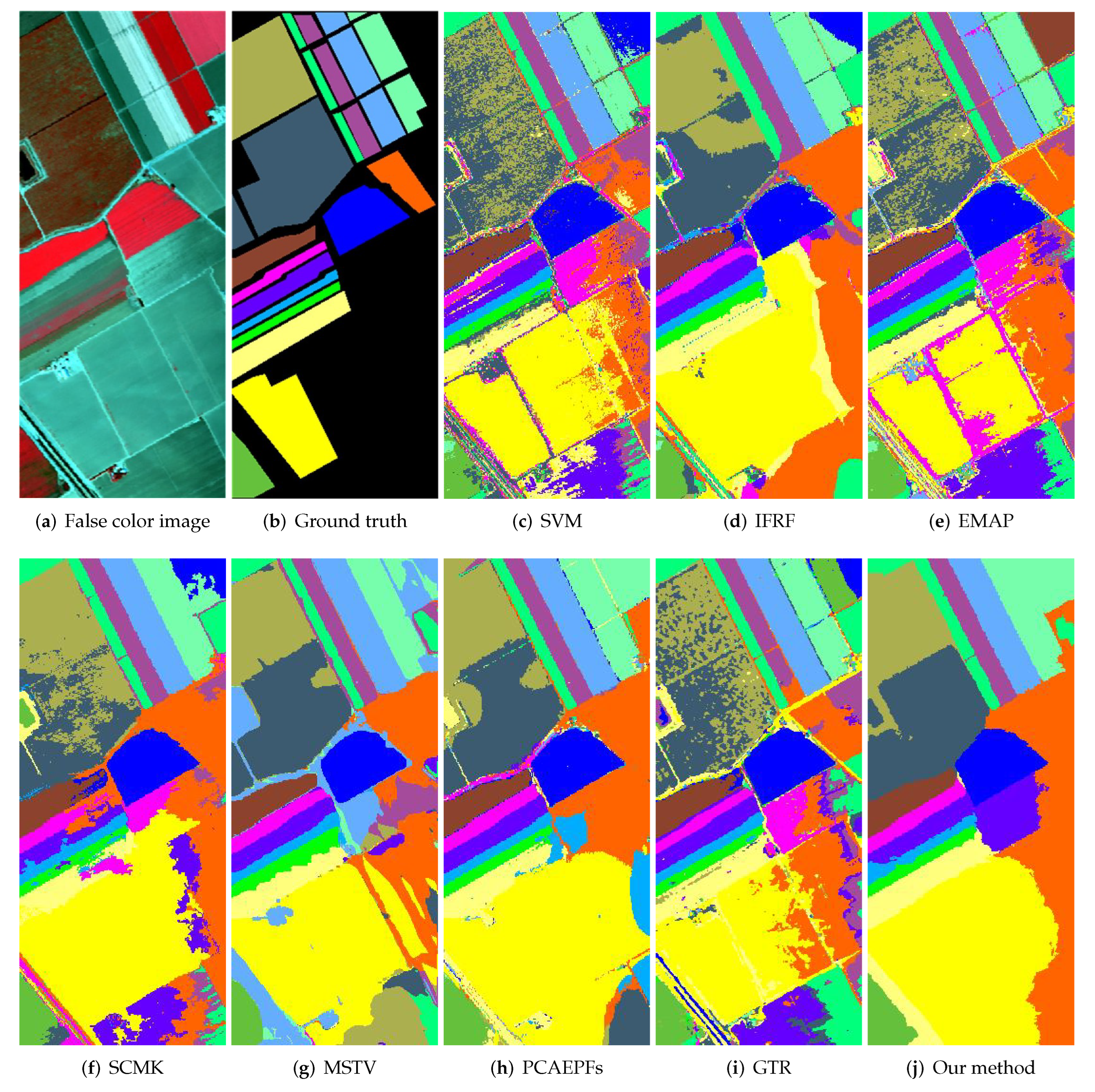
3.2.2. Salinas Dataset
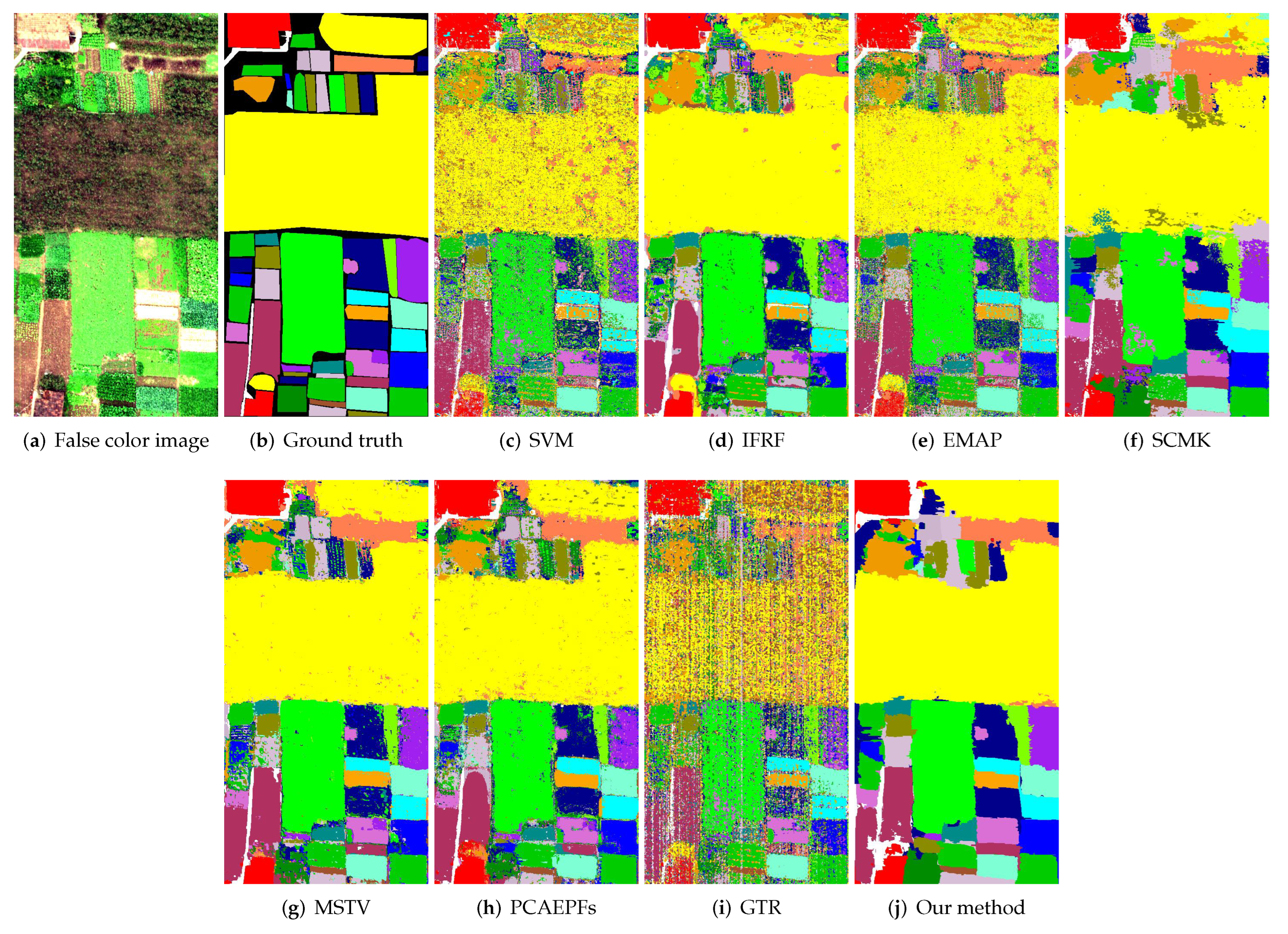
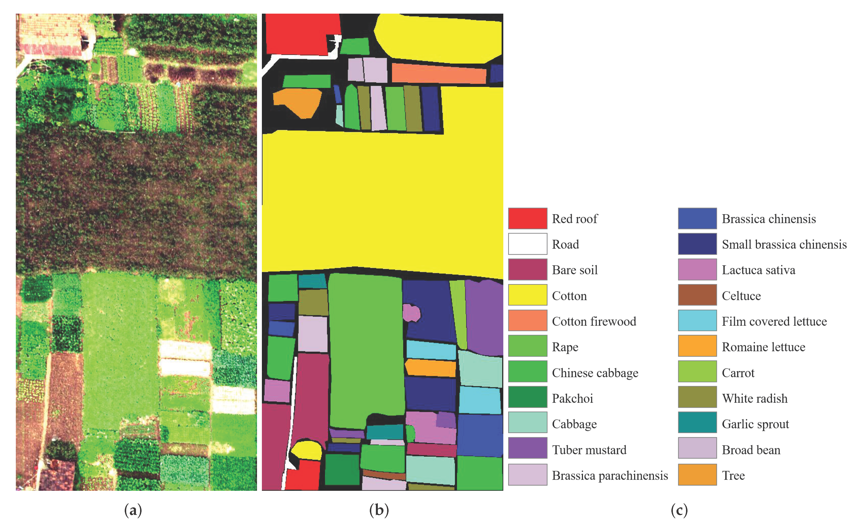
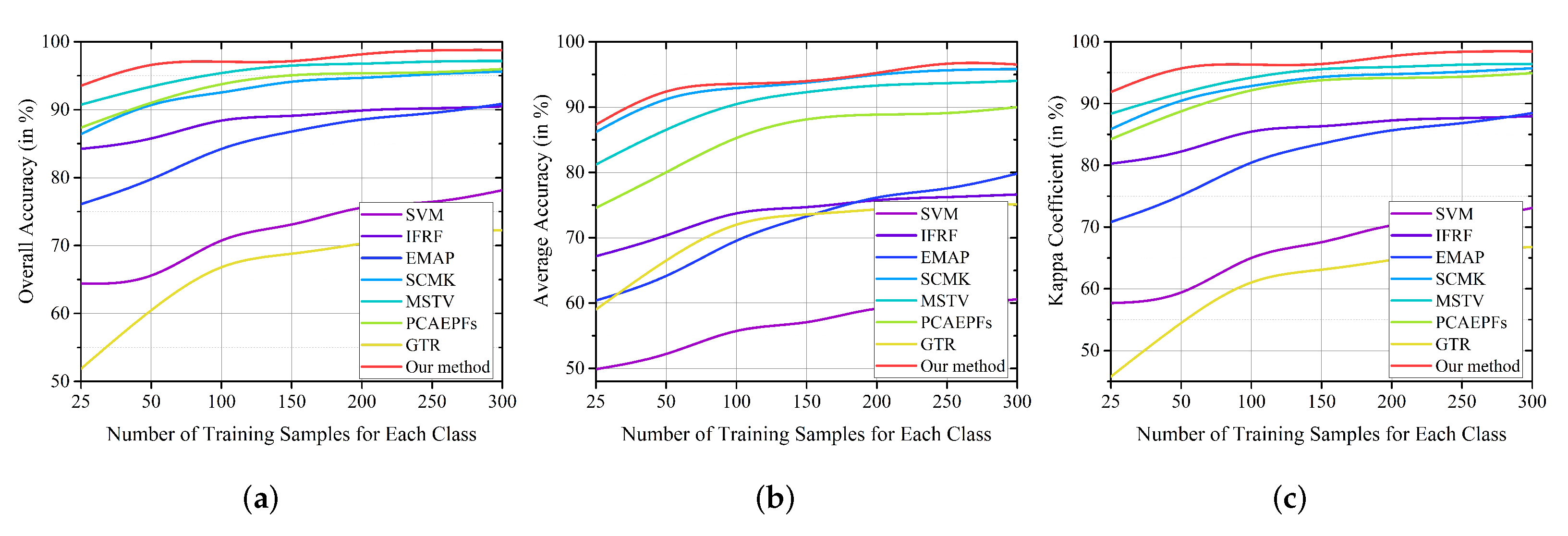
3.2.3. Honghu Dataset
4. Discussion
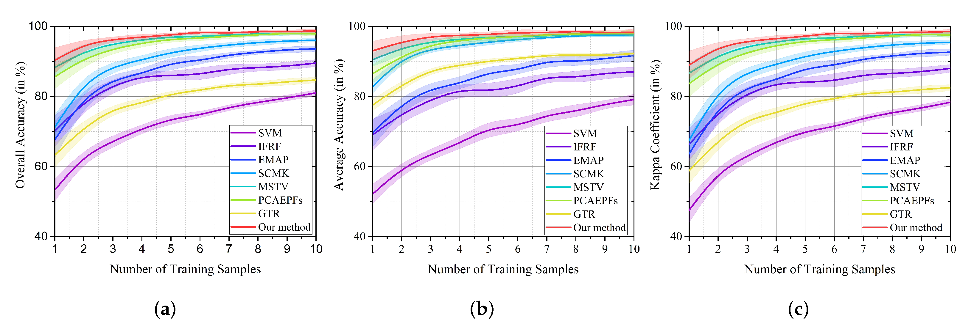
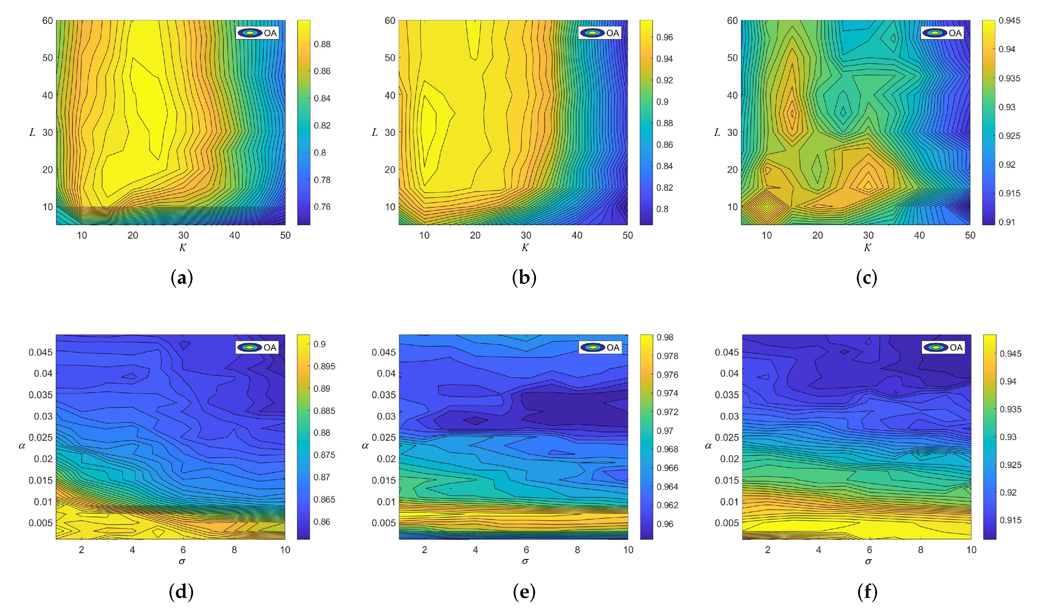
4.1. The Influence of Different Parameters
4.2. The Influence of Three Different Views
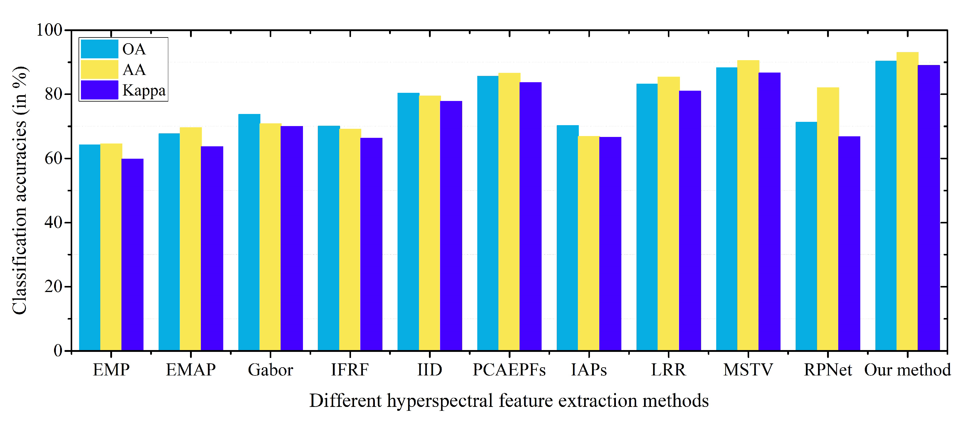
4.3. Effect of Different Hyperspectral Feature Methods
4.4. Computing Time
5. Conclusions
Author Contributions
Funding
Data Availability Statement
Acknowledgments
Conflicts of Interest
Abbreviations
| MNF | Minimum noise fraction |
| HSI | Hyperspectral image |
| PCA | Principal component analysis |
| ICA | Independent component analysis |
| APs | Attribute profiles |
| EMAP | Extended morphological attribute profiles |
| CNN | Convolutional neural network |
| ERS | Entropy rate superpixel |
| KPCA | Kernel PCA |
| SVM | Support vector machine |
| AVIRIS | Airborne Visible Infrared Imaging Spectrometer |
| CA | Class accuracy |
| OA | Overall accuracy |
| AA | Average accuracy |
| IFRF | Image fusion and recursive filtering |
| SCMK | Superpixel-based classification via multiple kernels |
| MSTV | Multi-scale total variation |
| PCAEPFs | PCA-based edge-preserving features |
| GTR | Generalized tensor regression |
| EMP | Extended morphological profiles |
| Gabor | Gabor filtering |
| IID | Intrinsic image decomposition |
| IAPs | Invariant attribute profiles |
| LRR | Low rank representation |
| RPNet | Random patches network |
References
- Rasti, B.; Hong, D.; Hang, R.; Ghamisi, P.; Kang, X.; Chanussot, J.; Benediktsson, J.A. Feature Extraction for Hyperspectral Imagery: The Evolution From Shallow to Deep: Overview and Toolbox. IEEE Geosci. Remote Sens. Mag. 2020, 8, 60–88. [Google Scholar] [CrossRef]
- Duan, P.; Lai, J.; Ghamisi, P.; Kang, X.; Jackisch, R.; Kang, J.; Gloaguen, R. Component Decomposition-Based Hyperspectral Resolution Enhancement for Mineral Mapping. Remote Sens. 2020, 12, 2903. [Google Scholar] [CrossRef]
- Liang, J.; Zhou, J.; Tong, L.; Bai, X.; Wang, B. Material Based Salient Object Detection from Hyperspectral Images. Pattern Recognit. 2018, 76, 476–490. [Google Scholar] [CrossRef] [Green Version]
- Li, S.; Zhang, K.; Duan, P.; Kang, X. Hyperspectral Anomaly Detection With Kernel Isolation Forest. IEEE Trans. Geosci. Remote Sens. 2020, 58, 319–329. [Google Scholar] [CrossRef]
- Duan, P.; Lai, J.; Kang, J.; Kang, X.; Ghamisi, P.; Li, S. Texture-Aware Total Variation-Based Removal of Sun Glint in Hyperspectral Images. ISPRS J. Photogramm. Remote Sens. 2020, 166, 359–372. [Google Scholar] [CrossRef]
- Stuart, M.B.; McGonigle, A.J.S.; Willmott, J.R. Hyperspectral Imaging in Environmental Monitoring: A Review of Recent Developments and Technological Advances in Compact Field Deployable Systems. Sensors 2019, 19, 3071. [Google Scholar] [CrossRef] [Green Version]
- Prasad, S.; Bruce, L.M. Limitations of Principal Components Analysis for Hyperspectral Target Recognition. IEEE Geosci. Remote Sens. Lett. 2008, 5, 625–629. [Google Scholar] [CrossRef]
- Kang, X.; Xiang, X.; Li, S.; Benediktsson, J.A. PCA-Based Edge-Preserving Features for Hyperspectral Image Classification. IEEE Trans. Geosci. Remote Sens. 2017, 55, 7140–7151. [Google Scholar] [CrossRef]
- Wang, J.; Chang, C.I. Independent Component Analysis-Based Dimensionality Reduction with Applications in Hyperspectral Image Analysis. IEEE Trans. Geosci. Remote Sens. 2006, 44, 1586–1600. [Google Scholar] [CrossRef]
- Gao, L.; Zhao, B.; Jia, X.; Liao, W.; Zhang, B. Optimized Kernel Minimum Noise Fraction Transformation for Hyperspectral Image Classification. Remote Sens. 2017, 9, 548. [Google Scholar] [CrossRef] [Green Version]
- Zhang, Y.; Kang, X.; Li, S.; Duan, P.; Benediktsson, J.A. Feature Extraction from Hyperspectral Images using Learned Edge Structures. Remote Sens. Lett. 2019, 10, 244–253. [Google Scholar] [CrossRef]
- Marpu, P.R.; Pedergnana, M.; Dalla Mura, M.; Benediktsson, J.A.; Bruzzone, L. Automatic Generation of Standard Deviation Attribute Profiles for Spectral–Spatial Classification of Remote Sensing Data. IEEE Geosci. Remote Sens. Lett. 2013, 10, 293–297. [Google Scholar] [CrossRef]
- Dalla Mura, M.; Villa, A.; Benediktsson, J.A.; Chanussot, J.; Bruzzone, L. Classification of Hyperspectral Images by Using Extended Morphological Attribute Profiles and Independent Component Analysis. IEEE Geosci. Remote Sens. Lett. 2011, 8, 542–546. [Google Scholar] [CrossRef] [Green Version]
- Kang, X.; Li, S.; Benediktsson, J.A. Feature Extraction of Hyperspectral Images With Image Fusion and Recursive Filtering. IEEE Trans. Geosci. Remote Sens. 2014, 52, 3742–3752. [Google Scholar] [CrossRef]
- Duan, P.; Kang, X.; Li, S.; Ghamisi, P. Noise-Robust Hyperspectral Image Classification via Multi-Scale Total Variation. IEEE J. Sel. Top. Appl. Earth Obs. Remote Sens. 2019, 12, 1948–1962. [Google Scholar] [CrossRef]
- Duan, P.; Ghamisi, P.; Kang, X.; Rasti, B.; Li, S.; Gloaguen, R. Fusion of Dual Spatial Information for Hyperspectral Image Classification. IEEE Trans. Geosci. Remote Sens. 2021, 59, 7726–7738. [Google Scholar] [CrossRef]
- Xia, J.; Bombrun, L.; Adalı, T.; Berthoumieu, Y.; Germain, C. Spectral–Spatial Classification of Hyperspectral Images Using ICA and Edge-Preserving Filter via an Ensemble Strategy. IEEE Trans. Geosci. Remote Sens. 2016, 54, 4971–4982. [Google Scholar] [CrossRef] [Green Version]
- Cui, B.; Xie, X.; Hao, S.; Cui, J.; Lu, Y. Semi-Supervised Classification of Hyperspectral Images Based on Extended Label Propagation and Rolling Guidance Filtering. Remote Sens. 2018, 10, 515. [Google Scholar] [CrossRef] [Green Version]
- Sellars, P.; Aviles-Rivero, A.I.; Schönlieb, C.B. Superpixel Contracted Graph-Based Learning for Hyperspectral Image Classification. IEEE Trans. Geosci. Remote Sens. 2020, 58, 4180–4193. [Google Scholar] [CrossRef] [Green Version]
- Li, Y.; Lu, T.; Li, S. Subpixel-Pixel-Superpixel-Based Multiview Active Learning for Hyperspectral Images Classification. IEEE Trans. Geosci. Remote Sens. 2020, 58, 4976–4988. [Google Scholar] [CrossRef]
- Li, Q.; Zheng, B.; Yang, Y. Spectral-Spatial Active Learning With Structure Density for Hyperspectral Classification. IEEE Access 2021, 9, 61793–61806. [Google Scholar] [CrossRef]
- Chen, Y.; Jiang, H.; Li, C.; Jia, X.; Ghamisi, P. Deep Feature Extraction and Classification of Hyperspectral Images Based on Convolutional Neural Networks. IEEE Trans. Geosci. Remote Sens. 2016, 54, 6232–6251. [Google Scholar] [CrossRef] [Green Version]
- Liu, B.; Yu, X.; Zhang, P.; Yu, A.; Fu, Q.; Wei, X. Supervised Deep Feature Extraction for Hyperspectral Image Classification. IEEE Trans. Geosci. Remote Sens. 2018, 56, 1909–1921. [Google Scholar] [CrossRef]
- Kang, X.; Zhuo, B.; Duan, P. Dual-Path Network-Based Hyperspectral Image Classification. IEEE Geosci. Remote Sens. Lett. 2019, 16, 447–451. [Google Scholar] [CrossRef]
- Xie, Z.; Hu, J.; Kang, X.; Duan, P.; Li, S. Multi-Layer Global Spectral-Spatial Attention Network for Wetland Hyperspectral Image Classification. IEEE Trans. Geosci. Remote Sens. 2021, 58, 3232–3245. [Google Scholar]
- Hang, R.; Li, Z.; Liu, Q.; Ghamisi, P.; Bhattacharyya, S.S. Hyperspectral Image Classification With Attention-Aided CNNs. IEEE Trans. Geosci. Remote Sens. 2021, 59, 2281–2293. [Google Scholar] [CrossRef]
- Hong, D.; Han, Z.; Yao, J.; Gao, L.; Zhang, B.; Plaza, A.; Chanussot, J. SpectralFormer: Rethinking Hyperspectral Image Classification with Transformers. IEEE Trans. Geosci. Remote Sens. 2022, 60, 1–15. [Google Scholar] [CrossRef]
- Duan, P.; Xie, Z.; Kang, X.; Li, S. Self-Supervised Learning-Based Oil Spill Detection of Hyperspectral Images. Sci. China Technol. Sci. 2022, 65, 793–801. [Google Scholar] [CrossRef]
- Xu, X.; Li, J.; Li, S. Multiview Intensity-Based Active Learning for Hyperspectral Image Classification. IEEE Trans. Geosci. Remote Sens. 2018, 56, 669–680. [Google Scholar] [CrossRef]
- Zhou, X.; Prasad, S.; Crawford, M.M. Wavelet-Domain Multiview Active Learning for Spatial-Spectral Hyperspectral Image Classification. IEEE J. Sel. Top. Appl. Earth Obs. Remote Sens. 2016, 9, 4047–4059. [Google Scholar] [CrossRef]
- Green, A.; Berman, M.; Switzer, P.; Craig, M. A Transformation for Ordering Multispectral Data in terms of Image Quality with Implications for Noise Removal. IEEE Trans. Geosci. Remote Sens. 1988, 26, 65–74. [Google Scholar] [CrossRef] [Green Version]
- Xu, L.; Yan, Q.; Xia, Y.; Jia, J. Structure Extraction from Texture via Relative Total Variation. ACM Trans. Graph. 2012, 31, 1–10. [Google Scholar] [CrossRef]
- Liu, M.Y.; Tuzel, O.; Ramalingam, S.; Chellappa, R. Entropy-Rate Clustering: Cluster Analysis via Maximizing a Submodular Function Subject to a Matroid Constraint. IEEE Trans. Pattern Anal. Mach. Intell. 2014, 36, 99–112. [Google Scholar] [CrossRef] [PubMed]
- Schölkopf, B.; Smola, A.; Müller, K.R. Kernel Principal Component Analysis. In Artificial Neural Networks—ICANN’97, Proceedings of the 7th International Conference, Lausanne, Switzerland, 8–10 October 1997 Proceeedings; Gerstner, W., Germond, A., Hasler, M., Nicoud, J.D., Eds.; Springer: Berlin/Heidelberg, Germany, 1997; pp. 583–588. [Google Scholar]
- Duan, P.; Kang, X.; Li, S.; Ghamisi, P.; Benediktsson, J.A. Fusion of Multiple Edge-Preserving Operations for Hyperspectral Image Classification. IEEE Trans. Geosci. Remote Sens. 2019, 57, 10336–10349. [Google Scholar] [CrossRef]
- Duan, P.; Kang, X.; Li, S.; Ghamisi, P. Multichannel Pulse-Coupled Neural Network-Based Hyperspectral Image Visualization. IEEE Trans. Geosci. Remote Sens. 2020, 58, 2444–2456. [Google Scholar] [CrossRef]
- Hang, R.; Liu, Q.; Hong, D.; Ghamisi, P. Cascaded Recurrent Neural Networks for Hyperspectral Image Classification. IEEE Trans. Geosci. Remote Sens. 2019, 57, 5384–5394. [Google Scholar] [CrossRef] [Green Version]
- Melgani, F.; Bruzzone, L. Classification of Hyperspectral Remote Sensing Images with Support Vector Machines. IEEE Trans. Geosci. Remote Sens. 2004, 42, 1778–1790. [Google Scholar] [CrossRef] [Green Version]
- Fang, L.; Li, S.; Duan, W.; Ren, J.; Benediktsson, J.A. Classification of Hyperspectral Images by Exploiting Spectral–Spatial Information of Superpixel via Multiple Kernels. IEEE Trans. Geosci. Remote Sens. 2015, 53, 6663–6674. [Google Scholar] [CrossRef] [Green Version]
- Liu, J.; Wu, Z.; Xiao, L.; Sun, J.; Yan, H. Generalized Tensor Regression for Hyperspectral Image Classification. IEEE Trans. Geosci. Remote Sens. 2020, 58, 1244–1258. [Google Scholar] [CrossRef]
- Benediktsson, J.; Palmason, J.; Sveinsson, J. Classification of Hyperspectral Data from Urban Areas Based on Extended Morphological Profiles. IEEE Trans. Geosci. Remote Sens. 2005, 43, 480–491. [Google Scholar] [CrossRef]
- He, L.; Li, J.; Plaza, A.; Li, Y. Discriminative Low-Rank Gabor Filtering for Spectral–Spatial Hyperspectral Image Classification. IEEE Trans. Geosci. Remote Sens. 2017, 55, 1381–1395. [Google Scholar] [CrossRef]
- Kang, X.; Li, S.; Fang, L.; Benediktsson, J.A. Intrinsic Image Decomposition for Feature Extraction of Hyperspectral Images. IEEE Trans. Geosci. Remote Sens. 2015, 53, 2241–2253. [Google Scholar] [CrossRef]
- Hong, D.; Wu, X.; Ghamisi, P.; Chanussot, J.; Yokoya, N.; Zhu, X.X. Invariant Attribute Profiles: A Spatial-Frequency Joint Feature Extractor for Hyperspectral Image Classification. IEEE Trans. Geosci. Remote Sens. 2020, 58, 3791–3808. [Google Scholar] [CrossRef] [Green Version]
- Rasti, B.; Ulfarsson, M.O.; Sveinsson, J.R. Hyperspectral Feature Extraction Using Total Variation Component Analysis. IEEE Trans. Geosci. Remote Sens. 2016, 54, 6976–6985. [Google Scholar] [CrossRef]
- Xu, Y.; Du, B.; Zhang, F.; Zhang, L. Hyperspectral Image Classification via a Random Patches Network. ISPRS J. Photogramm. Remote Sens. 2018, 142, 344–357. [Google Scholar] [CrossRef]


| No. | Indian Pines Dataset | Salinas Dataset | Honghu Dataset | ||||||
|---|---|---|---|---|---|---|---|---|---|
| Name | Train | Test | Name | Train | Test | Name | Train | Test | |
| 1 | Alfalfa | 6 | 40 | Weeds_1 | 5 | 2004 | Red roof | 25 | 14,016 |
| 2 | Corn_N | 7 | 1421 | Weeds_2 | 5 | 3721 | Road | 25 | 3487 |
| 3 | Corn_M | 6 | 824 | Fallow | 5 | 1971 | Bare soil | 25 | 21,796 |
| 4 | Corn | 6 | 231 | Fallow_P | 5 | 1389 | Cotton | 25 | 163,260 |
| 5 | Grass_M | 6 | 477 | Fallow_S | 5 | 2673 | Cotton firewood | 25 | 6193 |
| 6 | Grass_T | 6 | 724 | Stubble | 5 | 3954 | Rape | 25 | 44,532 |
| 7 | Grass_P | 6 | 22 | Celery | 5 | 3574 | Chinese cabbage | 25 | 24,078 |
| 8 | Hay_W | 7 | 471 | Grapes | 5 | 11,266 | Packchoi | 25 | 4029 |
| 9 | Oats | 6 | 14 | Soil | 5 | 6198 | Cabbage | 25 | 10,794 |
| 10 | Soybean_N | 7 | 965 | Corn | 5 | 3273 | Tuber mustard | 25 | 12,369 |
| 11 | Soybean_M | 8 | 2447 | Lettuce_4 | 5 | 1063 | Brassica parachinensis | 25 | 10,990 |
| 12 | Soybean_C | 6 | 587 | Lettuce_5 | 5 | 1922 | Brassica chinensis | 25 | 8929 |
| 13 | Wheat | 6 | 199 | Lettuce_6 | 5 | 911 | Small Brassica chinensis | 25 | 22,482 |
| 14 | Woods | 6 | 1259 | Lettuce_7 | 5 | 1065 | Lactuca sativa | 25 | 7331 |
| 15 | Buildings | 6 | 380 | Vinyard_U | 5 | 7263 | Celtuce | 25 | 977 |
| 16 | Stone | 7 | 86 | Vinyard_T | 5 | 1802 | Film covered | 25 | 7237 |
| 17 | Total | 102 | 10,147 | Total | 80 | 54,049 | Romaine lettuce | 25 | 2985 |
| 18 | Carrot | 25 | 3192 | ||||||
| 19 | White radish | 25 | 8687 | ||||||
| 20 | Garlic sprout | 25 | 3461 | ||||||
| 21 | Broad bean | 25 | 1303 | ||||||
| 22 | Tree | 25 | 4015 | ||||||
| Total | 550 | 386,143 | |||||||
| Class | SVM | IFRF | EMAP | SCMK | MSTV | PCAEPFs | GTR | Our Method |
|---|---|---|---|---|---|---|---|---|
| 1 | 31.53 (9.74) | 63.03 (27.93) | 94.21 (9.19) | 98.00 (1.05) | 95.92 (10.41) | 98.02 (4.65) | 96.75 (2.06) | 100.0 (0.00) |
| 2 | 47.00 (6.00) | 70.64 (15.98) | 59.74 (8.25) | 60.27 (11.34) | 86.93 (5.35) | 76.38 (7.21) | 55.64 (8.15) | 86.37 (5.87) |
| 3 | 34.03 (14.66) | 48.62 (12.35) | 53.23 (13.54) | 57.23 (13.07) | 71.01 (8.26) | 73.79 (13.56) | 47.42 (8.58) | 83.07 (16.27) |
| 4 | 26.70 (6.66) | 52.45 (11.34) | 36.54 (6.17) | 94.42 (4.94) | 67.17 (9.51) | 66.83 (7.53) | 72.47 (11.74) | 86.05 (10.51) |
| 5 | 63.24 (9.75) | 75.81 (10.59) | 67.96 (10.27) | 78.97 (12.76) | 97.49 (3.45) | 93.86 (6.29) | 83.06 (9.97) | 98.30 (3.94) |
| 6 | 79.83 (8.04) | 91.26 (4.32) | 90.31 (3.84) | 89.78 (11.19) | 98.70 (2.05) | 94.28 (3.29) | 88.07 (5.81) | 99.96 (0.13) |
| 7 | 31.35 (14.53) | 57.65 (21.85) | 61.05 (20.27) | 97.27 (2.35) | 98.70 (2.10) | 73.05 (31.40) | 99.09 (2.87) | 80.73 (25.62) |
| 8 | 95.57 (2.12) | 99.89 (0.27) | 100.0 (0.00) | 100.0 (0.00) | 100.0 (0.00) | 100.0 (0.00) | 88.77 (7.52) | 100.0 (0.00) |
| 9 | 17.18 (8.59) | 28.91 (13.60) | 40.28 (10.36) | 100.0 (0.00) | 96.67 (10.54) | 72.87 (21.18) | 98.57 (4.52) | 98.08 (4.27) |
| 10 | 41.51 (5.35) | 66.42 (8.13) | 52.5 (10.53) | 67.95 (13.90) | 81.22 (9.40) | 78.55 (10.42) | 54.30 (8.60) | 90.70 (8.08) |
| 11 | 60.65 (8.31) | 73.91 (6.22) | 75.15 (9.85) | 59.69 (9.88) | 92.28 (4.04) | 90.14 (4.52) | 41.52 (11.20) | 89.40 (6.90) |
| 12 | 29.10 (5.43) | 56.65 (9.17) | 48.07 (5.31) | 65.54 (9.57) | 78.81 (12.25) | 77.19 (12.22) | 67.00 (8.52) | 83.81 (15.76) |
| 13 | 79.14 (3.12) | 74.79 (12.60) | 85.46 (9.48) | 100.0 (0.00) | 100.0 (0.00) | 97.45 (4.78) | 99.25 (1.09) | 100.0 (0.00) |
| 14 | 88.92 (5.36) | 93.03 (4.09) | 91.79 (4.98) | 81.92 (9.64) | 99.54 (0.65) | 99.66 (0.45) | 85.77 (9.36) | 99.61 (0.24) |
| 15 | 33.04 (7.36) | 59.07 (13.37) | 65.61 (14.81) | 76.47 (11.34) | 89.69 (10.56) | 93.72 (5.04) | 65.53 (11.80) | 93.78 (6.94) |
| 16 | 76.05 (19.59) | 93.16 (5.08) | 90.53 (7.63) | 97.79 (0.37) | 93.82 (3.82) | 98.37 (1.07) | 97.67 (4.17) | 98.80 (0.02) |
| OA | 53.30 (3.23) | 70.09 (4.51) | 67.70 (5.14) | 71.20 (3.52) | 88.25 (2.45) | 85.58 (3.35) | 63.25 (3.46) | 90.32 (3.58) |
| AA | 52.18 (2.78) | 69.08 (4.43) | 69.53 (3.88) | 82.83 (1.89) | 90.49 (1.93) | 86.51 (2.53) | 77.55 (1.61) | 93.04 (2.75) |
| Kappa | 47.57 (3.44) | 66.35 (4.72) | 63.67 (5.52) | 67.50 (3.90) | 86.63 (2.77) | 83.65 (3.75) | 58.79 (3.59) | 88.96 (4.02) |
| Classes | SVM | IFRF | EMAP | SCMK | MSTV | PCAEPFs | GTR | Our Method |
|---|---|---|---|---|---|---|---|---|
| 1 | 99.13 (0.97) | 99.95 (0.16) | 99.98 (0.05) | 97.53 (5.50) | 100.0 (0.00) | 100.0 (0.00) | 97.33 (2.25) | 100.0 (0.00) |
| 2 | 98.74 (1.00) | 98.66 (1.31) | 99.75 (0.14) | 98.90 (3.48) | 99.97 (0.05) | 99.95 (0.08) | 99.84 (0.32) | 100.0 (0.00) |
| 3 | 79.50 (8.77) | 98.34 (1.93) | 94.55 (2.25) | 96.40 (7.65) | 97.87 (2.83) | 97.72 (2.38) | 85.58 (8.80) | 99.47 (0.10) |
| 4 | 96.00 (2.41) | 91.59 (3.95) | 95.93 (1.39) | 90.01 (8.71) | 96.90 (1.79) | 93.19 (4.02) | 99.83 (0.07) | 97.03 (0.28) |
| 5 | 94.01 (7.06) | 97.08 (1.77) | 96.66 (6.27) | 97.93 (1.56) | 96.86 (1.49) | 98.98 (3.21) | 90.12 (6.82) | 99.96 (0.01) |
| 6 | 99.79 (0.53) | 100.0 (0.00) | 99.41 (0.73) | 99.75 (0.00) | 98.34 (2.92) | 99.98 (0.04) | 98.89 (2.86) | 99.97 (0.01) |
| 7 | 95.27 (3.61) | 97.43 (2.27) | 96.27 (3.16) | 99.85 (0.06) | 96.23 (5.52) | 99.92 (0.06) | 99.18 (0.65) | 99.83 (0.01) |
| 8 | 64.94 (4.82) | 91.99 (3.74) | 80.00 (7.80) | 69.96 (8.23) | 92.73 (5.95) | 93.66 (6.53) | 69.49 (11.96) | 98.22 (2.96) |
| 9 | 98.66 (0.87) | 98.95 (0.67) | 98.99 (0.21) | 99.91 (0.19) | 98.61 (1.03) | 99.58 (0.46) | 98.84 (0.95) | 99.33 (0.67) |
| 10 | 77.21 (6.38) | 97.51 (1.62) | 87.98 (4.27) | 82.44 (14.88) | 95.02 (7.28) | 99.31 (0.97) | 80.51 (10.31) | 98.98 (0.19) |
| 11 | 82.43 (10.35) | 93.20 (3.51) | 79.41 (10.37) | 94.93 (5.93) | 99.65 (0.78) | 95.04 (4.63) | 96.43 (2.38) | 97.42 (7.25) |
| 12 | 89.11 (7.96) | 94.98 (5.23) | 88.64 (6.36) | 91.05 (12.43) | 99.11 (1.13) | 94.71 (4.32) | 98.12 (5.45) | 98.62 (2.48) |
| 13 | 79.04 (12.81) | 83.39 (11.25) | 92.32 (3.45) | 93.94 (10.28) | 95.32 (6.68) | 91.81 (11.56) | 98.79 (0.71) | 81.85 (6.29) |
| 14 | 85.09 (12.77) | 84.15 (17.99) | 97.23 (1.08) | 88.92 (3.95) | 89.54 (10.17) | 92.54 (10.36) | 91.01 (5.19) | 94.81 (6.19) |
| 15 | 46.93 (5.71) | 70.34 (13.57) | 56.84 (7.75) | 82.66 (11.52) | 84.53 (7.06) | 84.52 (8.47) | 65.16 (14.05) | 95.59 (4.72) |
| 16 | 93.27 (5.57) | 99.12 (0.76) | 96.43 (2.26) | 93.83 (10.51) | 97.68 (4.67) | 99.96 (0.08) | 86.38 (7.44) | 100.0 (0.00) |
| OA | 80.08 (1.96) | 90.67 (3.33) | 85.54 (2.57) | 88.70 (2.84) | 94.46 (1.47) | 95.12 (1.37) | 85.59 (3.54) | 98.13 (0.59) |
| AA | 86.19 (1.07) | 93.54 (1.84) | 91.27 (1.07) | 92.38 (2.16) | 96.14 (1.18) | 96.30 (0.94) | 90.96 (1.67) | 97.57 (0.75) |
| Kappa | 77.87 (2.15) | 89.66 (3.65) | 83.97 (2.81) | 87.47 (3.15) | 93.84 (1.64) | 94.56 (1.53) | 83.97 (3.94) | 97.92 (0.67) |
| Classes | SVM | IFRF | EMAP | SCMK | MSTV | PCAEPFs | GTR | Our Method |
|---|---|---|---|---|---|---|---|---|
| 1 | 88.17 | 98.22 | 91.04 | 86.91 | 97.73 | 89.84 | 75.41 | 89.69 |
| 2 | 54.73 | 67.79 | 64.54 | 86.23 | 73.31 | 78.28 | 57.36 | 57.95 |
| 3 | 88.51 | 96.16 | 92.62 | 93.44 | 93.27 | 96.64 | 61.13 | 97.83 |
| 4 | 96.12 | 99.31 | 98.30 | 87.64 | 99.50 | 99.56 | 44.66 | 99.72 |
| 5 | 17.85 | 57.84 | 23.49 | 98.66 | 63.24 | 52.07 | 55.53 | 79.29 |
| 6 | 85.18 | 90.83 | 89.97 | 89.74 | 93.78 | 93.26 | 69.41 | 99.40 |
| 7 | 74.00 | 89.38 | 81.95 | 77.24 | 89.62 | 88.44 | 50.93 | 95.81 |
| 8 | 6.09 | 16.05 | 10.73 | 90.02 | 43.87 | 31.39 | 42.74 | 97.99 |
| 9 | 91.60 | 99.21 | 89.67 | 94.61 | 90.23 | 86.79 | 90.75 | 97.82 |
| 10 | 49.29 | 73.45 | 73.62 | 76.59 | 91.88 | 83.72 | 32.99 | 99.44 |
| 11 | 28.17 | 58.82 | 41.50 | 77.43 | 69.88 | 64.28 | 21.36 | 79.63 |
| 12 | 43.33 | 61.20 | 52.56 | 93.64 | 64.18 | 61.54 | 43.77 | 96.26 |
| 13 | 50.58 | 77.54 | 70.86 | 70.73 | 79.52 | 81.99 | 30.38 | 78.44 |
| 14 | 43.35 | 70.73 | 60.01 | 86.77 | 90.14 | 78.77 | 61.29 | 80.40 |
| 15 | 3.97 | 31.73 | 23.46 | 97.24 | 57.05 | 51.69 | 82.80 | 91.99 |
| 16 | 80.93 | 93.51 | 87.57 | 94.53 | 99.01 | 98.66 | 82.34 | 98.37 |
| 17 | 54.39 | 72.82 | 62.17 | 93.10 | 85.53 | 92.66 | 73.80 | 97.09 |
| 18 | 21.83 | 32.85 | 39.27 | 95.08 | 72.90 | 67.53 | 74.91 | 68.77 |
| 19 | 48.88 | 64.45 | 51.52 | 64.06 | 83.41 | 58.41 | 56.23 | 74.37 |
| 20 | 38.00 | 54.19 | 59.34 | 99.86 | 79.59 | 65.60 | 46.06 | 88.71 |
| 21 | 11.04 | 24.32 | 38.85 | 100.00 | 86.11 | 43.46 | 71.14 | 91.70 |
| 22 | 21.50 | 47.34 | 25.73 | 99.55 | 82.90 | 76.21 | 73.23 | 89.30 |
| OA | 64.43 | 84.23 | 76.11 | 86.41 | 90.74 | 87.37 | 51.87 | 94.01 |
| AA | 49.88 | 67.17 | 60.39 | 88.18 | 81.21 | 74.58 | 59.01 | 88.64 |
| Kappa | 57.68 | 80.27 | 70.82 | 85.86 | 88.37 | 84.23 | 45.79 | 92.47 |
| Local-View | Intra-View | Inter-View | OA | AA | Kappa | Time (s) |
|---|---|---|---|---|---|---|
| ✓ | 87.22 | 85.08 | 85.51 | 3.68 | ||
| ✓ | 86.22 | 86.78 | 84.38 | 3.87 | ||
| ✓ | 87.35 | 90.66 | 85.63 | 3.95 | ||
| ✓ | ✓ | 88.32 | 89.41 | 86.71 | 4.17 | |
| ✓ | ✓ | 88.96 | 91.21 | 87.43 | 4.31 | |
| ✓ | ✓ | 88.25 | 92.07 | 86.58 | 4.48 | |
| ✓ | ✓ | ✓ | 90.32 | 93.04 | 88.96 | 5.36 |
| Datasets | SVM | IFRF | EMAP | SCMK | MSTV | PCAEPFs | GTR | Our Method |
|---|---|---|---|---|---|---|---|---|
| Indian Pines | 5.53 | 2.32 | 3.25 | 4.49 | 4.35 | 2.67 | 2.04 | 5.36 |
| Salinas | 21.08 | 2.68 | 4.56 | 3.23 | 12.34 | 12.98 | 2.49 | 19.35 |
| Honghu | 128.26 | 16.55 | 69.94 | 15.75 | 45.67 | 20.79 | 9.37 | 102.23 |
Publisher’s Note: MDPI stays neutral with regard to jurisdictional claims in published maps and institutional affiliations. |
© 2022 by the authors. Licensee MDPI, Basel, Switzerland. This article is an open access article distributed under the terms and conditions of the Creative Commons Attribution (CC BY) license (https://creativecommons.org/licenses/by/4.0/).
Share and Cite
Liang, N.; Duan, P.; Xu, H.; Cui, L. Multi-View Structural Feature Extraction for Hyperspectral Image Classification. Remote Sens. 2022, 14, 1971. https://doi.org/10.3390/rs14091971
Liang N, Duan P, Xu H, Cui L. Multi-View Structural Feature Extraction for Hyperspectral Image Classification. Remote Sensing. 2022; 14(9):1971. https://doi.org/10.3390/rs14091971
Chicago/Turabian StyleLiang, Nannan, Puhong Duan, Haifeng Xu, and Lin Cui. 2022. "Multi-View Structural Feature Extraction for Hyperspectral Image Classification" Remote Sensing 14, no. 9: 1971. https://doi.org/10.3390/rs14091971
APA StyleLiang, N., Duan, P., Xu, H., & Cui, L. (2022). Multi-View Structural Feature Extraction for Hyperspectral Image Classification. Remote Sensing, 14(9), 1971. https://doi.org/10.3390/rs14091971