Article

Near-Surface and High-Resolution Satellite Time Series for Detecting Crop Phenology

Department of Geography and Geographic Information Science, University of Illinois at Urbana-Champaign, Urbana, IL 61801, USA
*
Author to whom correspondence should be addressed.
Remote Sens. 2022, 14(9), 1957; https://doi.org/10.3390/rs14091957
Submission received: 2 March 2022 / Revised: 15 April 2022 / Accepted: 17 April 2022 / Published: 19 April 2022

Abstract

:
Detecting crop phenology with satellite time series is important to characterize agroecosystem energy-water-carbon fluxes, manage farming practices, and predict crop yields. Despite the advances in satellite-based crop phenological retrievals, interpreting those retrieval characteristics in the context of on-the-ground crop phenological events remains a long-standing hurdle. Over the recent years, the emergence of near-surface phenology cameras (e.g., PhenoCams), along with the satellite imagery of both high spatial and temporal resolutions (e.g., PlanetScope imagery), has largely facilitated direct comparisons of retrieved characteristics to visually observed crop stages for phenological interpretation and validation. The goal of this study is to systematically assess near-surface PhenoCams and high-resolution PlanetScope time series in reconciling sensor- and ground-based crop phenological characterizations. With two critical crop stages (i.e., crop emergence and maturity stages) as an example, we retrieved diverse phenological characteristics from both PhenoCam and PlanetScope imagery for a range of agricultural sites across the United States. The results showed that the curvature-based Greenup and Gu-based Upturn estimates showed good congruence with the visually observed crop emergence stage (RMSE about 1 week, bias about 0–9 days, and R square about 0.65–0.75). The threshold- and derivative-based End of greenness falling Season (i.e., EOS) estimates reconciled well with visual crop maturity observations (RMSE about 5–10 days, bias about 0–8 days, and R square about 0.6–0.75). The concordance among PlanetScope, PhenoCam, and visual phenology demonstrated the potential to interpret the fine-scale sensor-derived phenological characteristics in the context of physiologically well-characterized crop phenological events, which paved the way to develop formal protocols for bridging ground-satellite phenological characterization.

1. Introduction

Vegetation phenology regulates the biosphere’s seasonal carbon, nutrient, and water dynamics, and is a first-order control on ecosystem processes and productivity [1,2,3,4]. It is also a sensitive indicator of the biological impacts of climate change and mediates vegetation feedbacks to the climate system by influencing the biogeochemical and physical processes (e.g., carbon sequestration, surface albedo, and energy balance) [5,6,7,8]. In agricultural systems, crop phenology maintains a crucial role in estimating crop net primary production and yields, modeling surface energy-water-carbon fluxes, and managing farming practices (e.g., irrigation scheduling, fertilizer management, and harvesting operations) [9,10,11]. These crop management activities largely depend on crop phenological development stages, as biochemical and physiological characteristics (e.g., light use efficiency) of crops differ seasonally along the growth trajectory [12]. The crops at different phenological stages exhibit divergent responses to environmental changes and weather anomalies [12,13,14]. For instance, the anthesis stage of corn is particularly susceptible to heat stress, and elevated temperature at this stage has damaging effects on the corn growth, causing subsequent yield loss [15,16]. As climate change is inclined to increase the frequency of heat stress and other extreme weather events, detecting the crop phenological progress throughout the season is critical in supporting resilient and sustainable agricultural development.
Time series of satellite imagery facilitates the characterization of crop phenological patterns over space and time and expands the scope of crop phenological monitoring beyond traditional field observations [17,18,19]. The remotely sensed spectral reflectances and derived vegetation indices across the electromagnetic regions have been widely studied to track the seasonal dynamics of crop growth, and to derive critical phenological transition dates (e.g., onset of greenness) in association with crop biological growth stages (e.g., crop emergence) [20,21]. Specifically, a range of curve-fitting-based phenological models has been developed to smooth the satellite time series as well as to capture the seasonal variations in crop canopy development along the phenological trajectory [22]. Those curve-fitting-based models include the double logistic function and its variants, the Quadrat function, the Savitzky-Golay function, the Fourier transform (or harmonic) function, the wavelet function, the asymmetric Gaussian function, and the spline-relevant functions [23,24,25,26,27]. With the modeled seasonal dynamics through satellite time series, crop phenological transition dates characteristic of biological events of canopy phenology can further be extracted using phenophase analysis methods. The phenophase analysis methods include the threshold-based method (e.g., defined thresholds based on the curve amplitude), the curve derivative method (e.g., first and second derivatives of the curve), the curvature change rate method (e.g., extremes in curvature change rate of the curve), the moving average method (e.g., a departure from the moving average-based trend), and the pheno-network method (e.g., bridging coefficient in the phenology-tailored complex network) [28,29,30,31,32]. Those methods are designed to characterize distinct changes in canopy biophysical or biochemical properties that tend to be connected with crop phenophase transitions. In particular, Diao [19] developed a remote sensing phenological monitoring framework that systematically integrates a combination of curve-fitting and phenophase analysis methods for crop phenological characterization, and found that a range of corn and soybean phenological stages can be estimated under the devised framework with the phenological reference of district-level Crop Progress Reports (CPRs), the United States Department of Agriculture (USDA). To date, remotely sensed time series analysis of crop phenology has been mostly conducted at coarse spatial resolutions, as a tradeoff of the satellites (e.g., Moderate Resolution Imaging Spectroradiometer [MODIS]) to secure high temporal revisit rates for repeated monitoring. However, the pixels at coarse spatial resolutions may contain a heterogeneous matrix of agricultural fields with varying planted and harvested schedules, which confounds the crop phenological signal and makes it challenging to be connected to field-based crop phenological observations, particularly for smallholder and precision agricultural systems. The decoupling between satellite- and field-based phenological characterizations caused by the scale disparity has remained a significant hurdle in the phenological studies [33].
Over the recent years, near-surface remote sensing (e.g., digital repeat photography and Drone imagery) has emerged as valuable tools for bridging the gap between ground-based phenological observations at local scales and satellite-based phenological measures at ecosystem scales [34,35,36]. In particular, the North American PhenoCam network, initiated in 2008, is established to provide systematic and consistent canopy phenological monitoring with unifying observation protocols using digital cameras, and now includes more than 500 camera sites across different biomes [37,38,39]. Similar phenological camera networks have also been established in Europe (e.g., European Phenology Camera Network), Japan (e.g., Japanese Phenological Eyes Network), Australia (e.g., Australian PhenoCam Network), etc., [40,41,42]. Those phenological cameras can take repeated photos of vegetation in time-lapse mode (e.g., every 30 min from sunrise to sunset of the day) from a fixed position in the field to track vegetation dynamics throughout the season [43,44]. On one hand, the high-frequency digital repeat photography embodies rich color and structural information of vegetation to enable systematic visual phenological interpretations over the course of a year. On the other hand, the digital numbers recorded by the photography and derived indices (e.g., Green Chromatic Coordinate [GCC]) can be analyzed in a time series fashion, analogous to satellite time series phenological analysis, to track the canopy seasonal phenological development trajectory at the organism-to-ecosystem level. The phenophase transition dates (e.g., onset of greenness) can subsequently be extracted from such seasonal trajectory for sensor-based phenological characterizations [35,45]. With the dual potential roles, the phenological cameras have been explored to evaluate and validate the satellite-based (e.g., MODIS, Advanced Very High Resolution Radiometer (AVHRR), Visible Infrared Imaging Radiometer Suite (VIIRS), and Landsat) phenological measures, to refine the phenological and earth system models, and to study the vegetation responses to climate change [34,35,46,47,48,49,50,51]. Yet most of those near-surface remote sensing studies have been focused on forest and grassland ecosystems [35,46,47,48,50,51]. Little attention has been directed to assessing the linkage between sensor-derived phenological characteristics and visually observed crop growth stages in agricultural systems. Despite the fine-scale enhanced phenological monitoring, near-surface remote sensing may be limited by its spatial coverage, time span, and sensor geometry and configurations.
Apart from near-surface remote sensing, the accelerated development of satellite remote sensing opens up new opportunities to reconcile ground-level crop scouting and satellite-based agricultural phenological monitoring. During the past several years, the emergence of innovative satellite platforms, namely satellite constellations, has largely boosted our capability to monitor land surface dynamics. The PlanetScope satellite constellation (more than 130 CubeSats with the 3-unit form factor of 10 × 10 × 30 cm, and a mass of approximately 4 kg), launched by Planet Labs, can provide the near nadir-view coverage of the earth on a daily basis at fine spatial resolutions (i.e., 3–5 m spatial resolution) [52]. With the improved spatial and temporal characteristics, the PlanetScope imagery can potentially address the mixed phenology issue due to landscape heterogeneity under relatively coarse satellite spatial resolutions, as well as resolve the spatial coverage and potential sensor limitations of near-surface remote sensing [53,54,55,56]. It may shed light on how satellite-derived phenological measures can be aligned with field-observed crop phenological growth stages, particularly in spatially fragmented and heterogeneous landscapes. The PlanetScope time series has been found to improve the phenological characterizations in forest and rangeland systems [57,58,59,60]. In agricultural systems, this high-resolution imagery has been explored to detect the crop sowing and growth stages at the field scale [61,62]. However, there is still a dearth of research rigorously validating the crop phenological growth characterization results from this high-resolution imagery with regard to on-the-ground crop stage progress.
The goal of this study is to systematically assess near-surface phenological cameras and high-resolution satellite time series in reconciling sensor- and ground-based crop phenological characterizations. As the two most critical means to detect crop phenology at fine scales, near-surface and high-resolution remote sensing provide distinct yet complementary measures to facilitate direct comparisons to visually observed crop stages for phenological validations, a long-standing challenge in phenological studies. Specifically, we aim to (1) interpret the fine-scale sensor-derived phenological characteristics in the context of visually-observed crop phenological events, (2) evaluate the role of the near-surface phenological cameras in characterizing the crop phenological dynamics with a diverse range of corn and soybean PhenoCam sites, and (3) systematically compare a set of phenological measures from high-resolution PlanetScope imagery, PhenoCams, and visual observations for coupled ground and sensor-based crop growth characterizations. Despite the increasing use of PhenoCam-derived phenological metrics to validate satellite-based ones, the fine-scale crop phenological comparison between PhenoCam and PlanetScope imagery is lacking. The enhanced understanding of fine-scale phenological characterizations in association with ground crop growth observations will benefit more precise and sustainable stage-specific agricultural management, especially in spatially heterogeneous or smallholder agricultural systems.

2. Materials and Methods

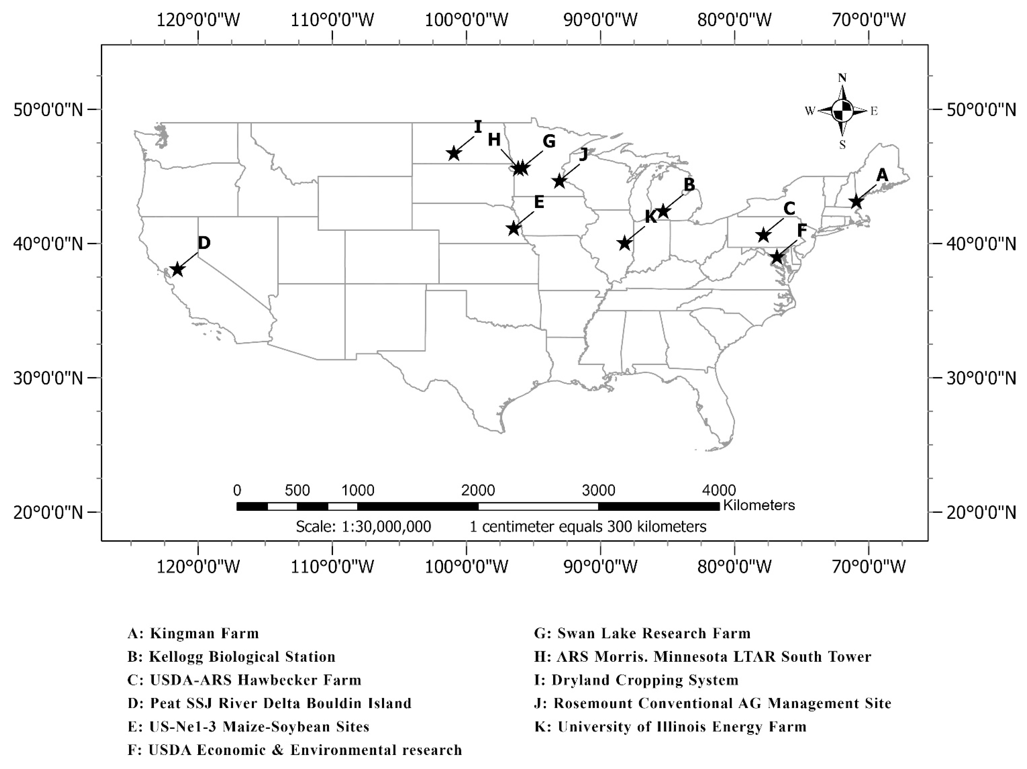
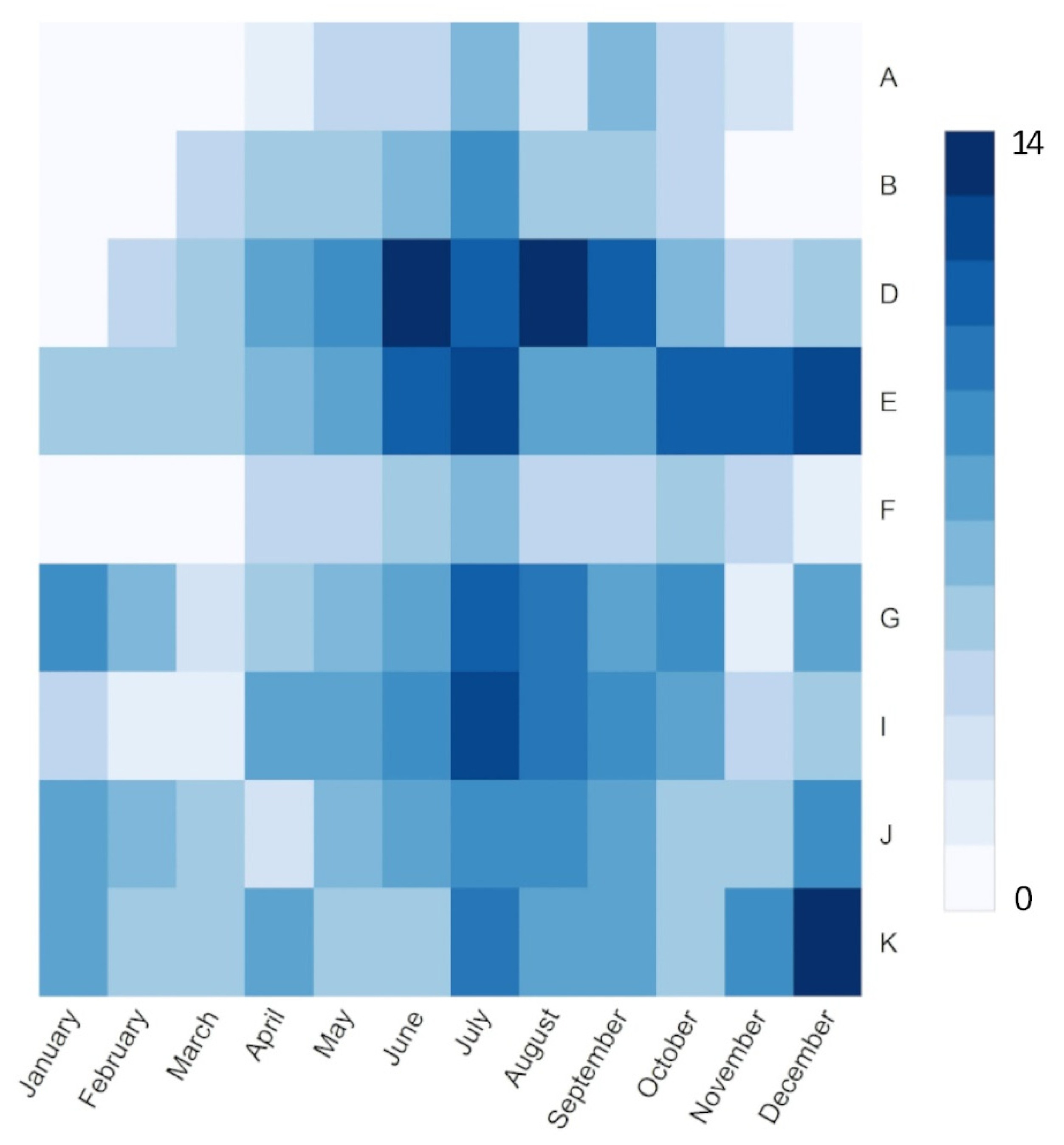
2.1. Study Sites and Data

As the two most cultivated crops in the US, corn, and soybean are selected for phenological characterization in this study. Our study sites comprise major corn and soybean sites in the US of the North American PhenoCam network, with longitudes spanning from 100.93°W to 121.54°W, and latitudes from 38.11°N to 46.76°N (Figure 1). The study sites include the Kingman Farm Site (Strafford County, NH, USA), Kellogg Biological Station Site (Barry County, MI, USA), USDA-ARS Hawbecker Farm Site (Huntingdon County, PA, USA), Peat SSJ River Delta Bouldin Island Site (San Joaquin County, CA, USA), US-Ne1-3 Maize-Soybean Site (Saunders County, NE, USA), USDA Economic and Environmental Research Site (Prince George’s County, MD, USA), Swan Lake Research Farm Site (Stevens County, MN, USA), ARS Morris Minnesota LTAR South Tower Site (Stevens County, MN, USA), Dryland Cropping System Site (Morton County, ND, USA), Rosemount Conventional AG Management Site (Dakota County, MN, USA), and University of Illinois Energy Farm Site (Champaign County, IL, USA) (Table 1). Those sites are selected with the careful assessment of the camera configuration (e.g., field of view and white balance), image availability and quality (e.g., illumination geometry and weather conditions), and site characteristics (e.g., cropping system and landscape homogeneity) [38,63].
The near-surface PhenoCam imagery of all the sites for the years 2010–2019 was acquired from the PhenoCam server (https://phenocam.sr.unh.edu/webcam/; accessed on 15 November 2020). The number of years for each site may vary, depending on the timing of site establishment. The PhenoCam imagery includes three bands (i.e., blue, green, and red), and provides the canopy-scale observation of crops, with each one taken about every 30 or 60 min throughout the year. In this study, only the images from 10:00 a.m. to 2:00 p.m. local time are considered to reduce the influence of illumination difference and atmospheric interference [44]. Most of the sites are type I or type II sites (Table 1). Type I sites utilize prescribed NetCam SC IR cameras (StarDot Technologies, Buena Park, CA, USA), and type II sites do not use the prescribed NetCam cameras. Yet for both site types, the cameras are generally deployed via a standardized phenological monitoring protocol with site personnel actively engaged in camera maintenance to ensure the image quality [38]. Specifically, the cameras are mounted to towers (or other secure points) taller than the crops of interest and are angled downward at 20–40° to obtain canopy views of the crops. The cameras are typically pointed north to minimize shadow and lens flare effects and are set to a fixed white balance to eliminate confounding variation in imaging sensor response. Some sites may contain several cameras, with each monitoring an agricultural field. For example, the US-Ne1-3 Maize-Soybean site has three cameras, which point to the US-Ne1 irrigated continuous maize field, the US-Ne2 irrigated maize-soybean rotation field, and the US-Ne3 rainfed maize-soybean rotation field, respectively. We then removed the site-years with images of relatively low quality or significant amount of missing data during the growing season to ensure the quality of PhenoCam observations. In total, there are 41 PhenoCam site-year observations for corn, and 16 PhenoCam site-year observations for soybean.
Besides the PhenoCam imagery, we also acquired the PlanetScope surface reflectance (Version 2.0) time series of the study sites from 2017 to 2019. The PlanetScope imagery is under the near nadir-view and has four bands (i.e., blue, green, red, and near-infrared), with a 3.7 m average ground sample distance and daily revisit frequency. The PlanetScope imagery was atmospherically corrected to surface reflectance using the 6S atmospheric model by the Planet Labs and was then filtered using the associated quality assurance layer, followed by the visual inspection, to remove the images that were contaminated by snow, cloud, and cloud shadow. With the year-long PlanetScope time series available starting from 2017, the number of PlanetScope site-year observations is a subset of that of PhenoCam site-year ones. Across the study sites, there are 21 PlanetScope site-year observations for corn and 10 PlanetScope site-year observations for soybean. The average number of cloud-free PlanetScope images per month varies across the study sites, with about 6 to 10 images per month during the growing season for most of the sites (Figure 2).

2.2. Methodology

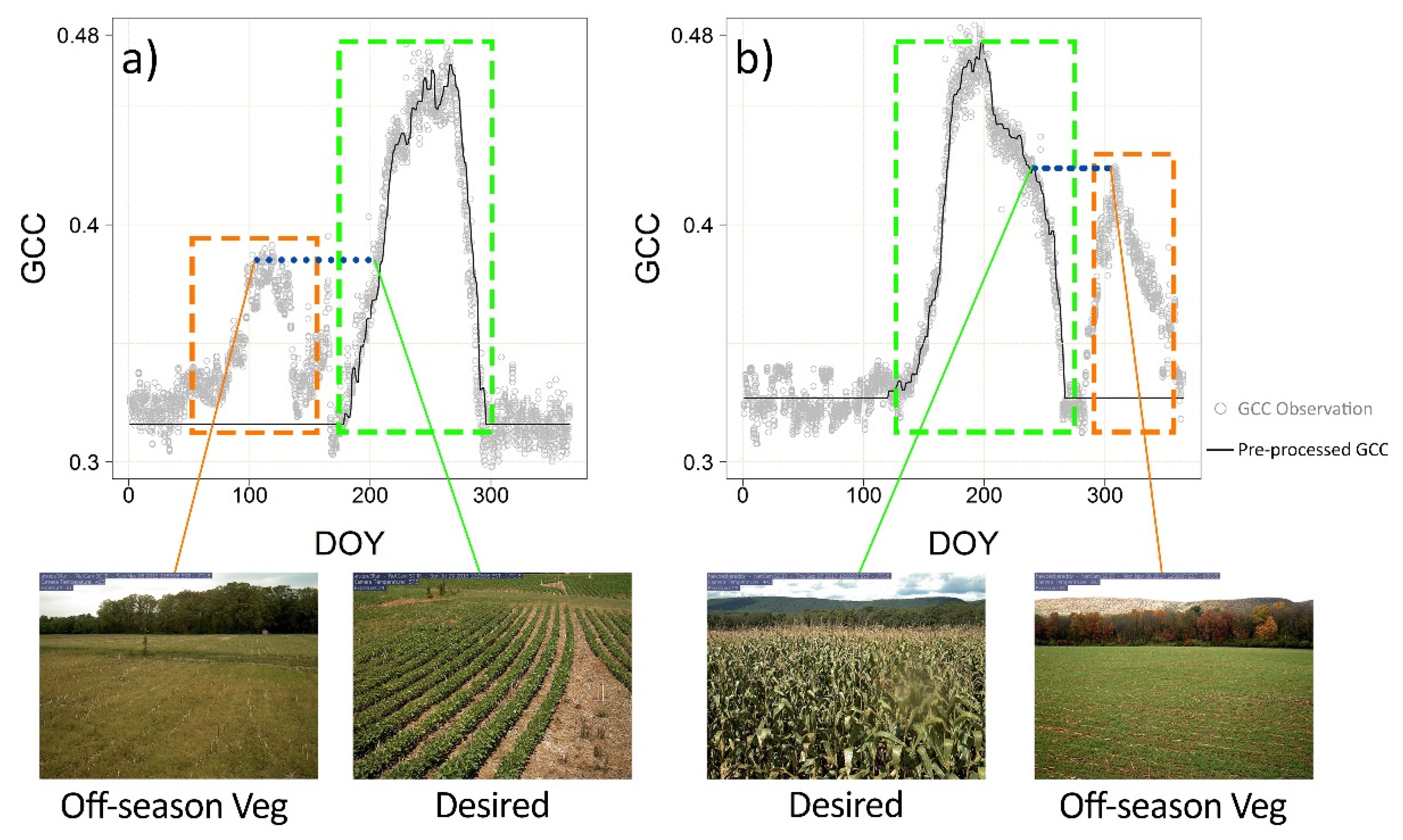
2.2.1. Imagery Pre-Processing

For the PhenoCam imagery of each study site, we first delineated a region of interest (ROI) of the crop canopy in the imagery for the subsequent phenological analysis. The ROI was delineated to cover the crop canopies located in the foreground of imagery to be representative of the broader landscape of each site while avoiding the non-target species (e.g., weed), soil, and sky. Delineation of an ROI in the foreground further diminished the effects of adverse weather conditions (e.g., cloud and fog), which could negatively affect the quality of characteristic phenology from PhenoCams [46]. The GCC time series of the ROI was then extracted from the imagery. GCC was calculated using Equation (1).
GCC = G D N R D N + G D N + B D N
Here, G D N , R D N , and B D N denote the average pixel digital numbers over the ROI for the green, red, and blue bands of the imagery, respectively.
GCC was developed to characterize the canopy greenness and had been extensively used in the RGB (red, green, and blue) imagery for monitoring canopy seasonal dynamics [37,63]. As GCC values tended to be reduced by snow or sub-optimal lighting conditions, we further generated the three-day composite using the 90th percentile value of GCC calculated over a three-day moving window to reduce the impacts of the variation in weather conditions, atmospheric interference, and illumination geometry [44]. As regards the PlanetScope imagery of each study site, we also delineated an ROI that took into account the corresponding PhenoCam location, PhenoCam orientation, and landscape characteristics, so the ROI in the PlanetScope imagery could approximate the crop canopy characteristics of that of the corresponding PhenoCam data. As the most widely used vegetation index, the normalized difference vegetation index (NDVI) was calculated from the PlanetScope ROI to generate the seasonal time series curves.
For both PhenoCam and PlanetScope, the extracted time series were subsequently filtered using the spline function to remove the outliers and spurious observations. The spline filter fitted a smoothing spline curve to the time series and detected the outliers based on the deviations from the curve. The degree of smoothing in the filter was determined using Akaike’s Information Criterion [38]. The resultant time series was further smoothed using the median of a three-point moving window to remove the remaining noise. The median smoothing was conducted iteratively until the time series became stable. During the dormant seasons, the time series might be affected by weeds, cover crops, etc., (Figure 3). The local fluctuations (e.g., orange box in Figure 3) caused by the off-season vegetation covers might confound the phenological patterns of the target crop species. We thus delimited the time series into segments, with each one representing a growth cycle, using the curve turning points (e.g., peaks and pits). The time series segments outside the growth cycle of the target crop species were replaced by the median dormant season values (e.g., the black curve in Figure 3). With the imagery pre-preprocessing, we attempted to remove the outliers and undesired off-season vegetation signals while retaining the seasonal phenological trajectory of the target crop species.

2.2.2. Crop Phenological Modeling

For both PhenoCam and PlanetScope imagery, the pre-processed time series was fitted using the Beck double logistic model [64]. The double logistic model had been widely utilized to model the vegetation phenological dynamics, as the parameters of the model could be linked with the characteristic phenological process [24]. The model could also capture the relatively short growing season of crops without overestimating the growing season duration [19]. Built on the double logistic model, the Beck model was employed in this study to model the pre-processed seasonal time series as a function of time using six unique parameters (Equation (2)).
V I ( t ) = w V I + ( m V I w V I ) × ( 1 1 + e ( a 1 × ( t a 2 ) ) + 1 1 + e ( b 1 × ( t b 2 ) ) 1 )
Here, VI(t) denotes the modeled value of a vegetation index (e.g., GCC or NDVI) at time t. wVI is the baseline value of the vegetation index during the dormant season and is determined through the imagery pre-processing (Section 2.2.1). mVI is the maximum value of the vegetation index throughout the growing season. a2 is the inflection point in the curve upward (or greening) direction and a1 controls the corresponding rate of curve increase at a2. Similarly, b2 is the inflection point in the curve downward (or senescing) direction and b1 denotes the corresponding rate of curve decrease at b2. The parameters in the Beck model were estimated using the iterative non-linear least squares.
The Beck double logistic model maintained two unique properties to improve the phenological modeling process. First, the Beck model replaced the dormant season vegetation index values lower than a pre-defined dormant value with that pre-defined one to reduce the impact of snow, ice, cloud, etc. In this study, the pre-defined dormant value was the median dormant season value of a vegetation index identified in image pre-processing (Section 2.2.1). Second, the Beck model incorporated a weighting factor that placed lighter weights on the values overestimated by the fitted model to diminish the influence of adverse weather conditions (e.g., sub-optimal illumination conditions) negatively biasing the observed values.
We also tested two other generalized double logistic models (e.g., Elmore and Klosterman models) with additional parameters considered for tracking the crop seasonal phenological dynamics [35,65]. The Elmore double logistic model could account for the declining trend of vegetation greenness in the summer months, while the Klosterman double logistic model took into account the varying changing rates near the asymptotes of the logistic functions as well as the changes of observation values during both dormant and summer periods. Despite the more generalized functions, these two models had degraded performance in our study sites compared to the Beck double logistic model, partly due to the lack of summer green-down process in certain agricultural sites or the increasingly large number of parameters to be optimized. Thus, the Beck double logistic model was employed in this study as the functional representation of phenological time series for retrieving the crop phenological transition dates.

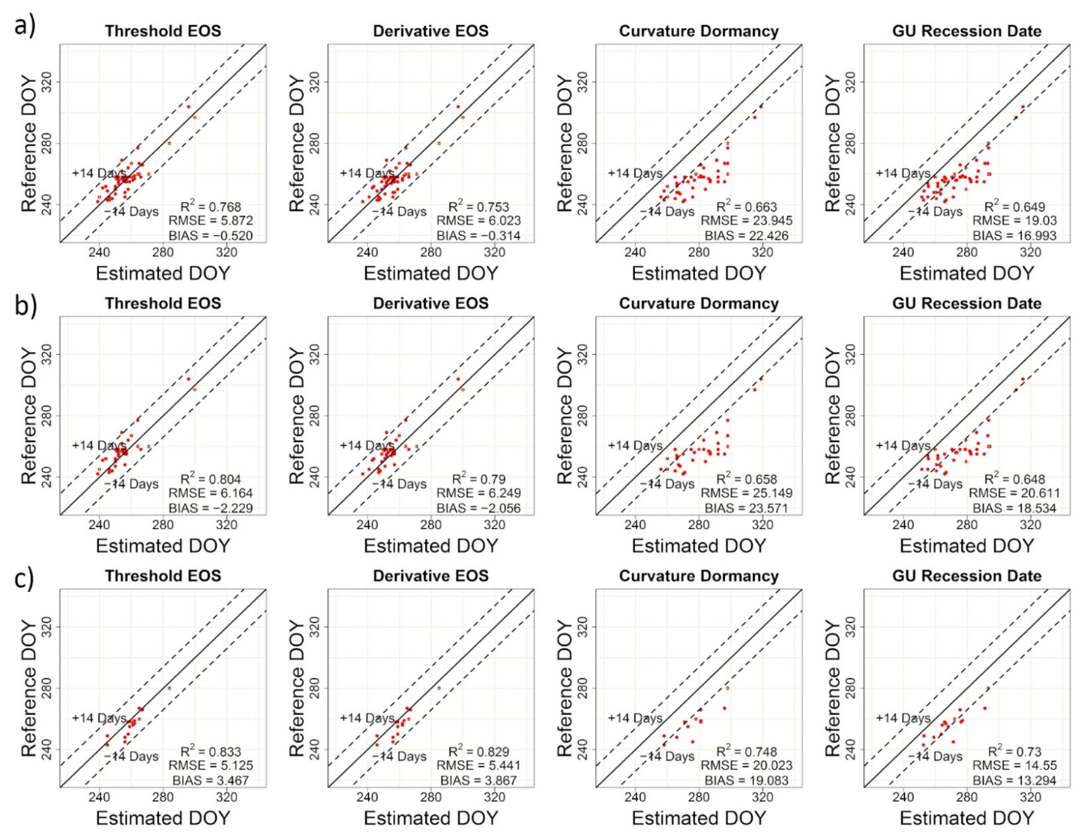
2.2.3. Crop Phenological Transition Date Analysis

With the Beck fitted time series, the phenological transition dates were then retrieved using four phenophase analysis methods, namely the time series threshold-based method (TRS-based method hereafter), the time series derivative-based method (DER-based method hereafter), the time series curvature-based method (CUR-based method hereafter), and the time series Gu-based method. For each of the methods, we retrieved relevant phenological metrics corresponding to the Start of greenness rising Season (i.e., SOS), as well as the metrics corresponding to the End of greenness falling Season (i.e., EOS). The retrieved metric-specific SOS would be compared with crop visual emergence observations, and the metric-specific EOS would be compared with crop visual maturity observations.
The TRS-based method identified critical phenophases by extracting the dates when the Beck fitted curve reached 50% of the seasonal amplitude of vegetation index. Due to the difficulty in arbitrarily defining a universal threshold applicable to different vegetation indices or crops of varying biophysical characteristics [17], we only tested 50% of the amplitude, a widely used threshold in phenological studies, in both curve upward and downward directions to represent the TRS-based SOS and EOS in this study. The DER-based method retrieved the phenological transition dates corresponding to the local extremes in the first derivative of the Beck fitted curve. The retrieved dates of maximum and minimum derivative values correspond to DER-based SOS and EOS, respectively. For the CUR-based method, it identified the local maxima/minima in the curvature change rate for the phenophase estimation [24]. During the greenness rising period, the CUR-based method extracted two phenological metrics, namely Greenup and Maturity, corresponding to the two local maxima in the change rate of the curvature. During the greenness falling period, it extracted another two phenological metrics, namely Senescence and Dormancy, corresponding to the two local minima in the curvature change rate. The Gu-based method extracted the phenological transition dates by leveraging the recovery, senescence, and boundary lines (i.e., base and plateau lines). The recovery line was a line tangent to the curve at the maximum point of the curve’s first derivative. Similarly, the senescence line was a line tangent to the curve at the minimum point of the first derivative. The base and plateau lines were the horizontal lines with median dormant season and maximum vegetation index values, respectively. During the greenness rising period, the Gu-based method extracted the Upturn Date (UD) and Stabilization Date (SD) phenological metrics by intersecting the recovery line with the base and plateau lines, respectively. During the greenness falling period, it retrieved the Downturn Date (DD) and Recession Date (RD) metrics by intersecting the senescence line with the plateau and the baselines, respectively. More information about the Gu-based phenological extraction could be found in Gu, et al. [66].
With the four phenophase analysis methods, a diverse range of metric-specific SOS and EOS characteristics of crop phenological transitioning could be retrieved. Specifically, the TRS-based SOS, DER-based SOS, CUR-based Greenup and Maturity, and Gu-based UD and SD metrics would be compared to the emerged stages of crops. The TRS-based EOS, DER-based EOS, CUR-based Senescence and Dormancy, and Gu-based DD and RD metrics would be compared to the mature stages of crops.

2.2.4. Accuracy Assessment

To assess the accuracy of PlanetScope and PhenoCam-retrieved crop phenological transition dates, we conducted visual interpretations of crop emergence and maturity for each site-year using the digital repeat photography of the PhenoCams. Compared to field-based phenological observations, the PhenoCam photos could enhance the temporal resolutions of observations, expand the geographical coverage, and reduce costs. In this study, the crop phenology of the 57 PhenoCam site-year observations was visually interpreted via a consistent protocol. Specifically, the crop emergence was interpreted when the crops were first visible within the defined ROI of the PhenoCam photos. The crop maturity was interpreted when the crop leaves were approximately 50% yellow within the ROI.
We evaluated the concordance among the PlanetScope, PhenoCam, and visually observed crop phenology using the statistical measures of root mean square error (RMSE), bias, and R square. These statistics quantified the magnitude of differences among the characteristic phenology, the average signed difference, and the degree of the variation in one type of phenological measurement explained by another, respectively.

3. Results

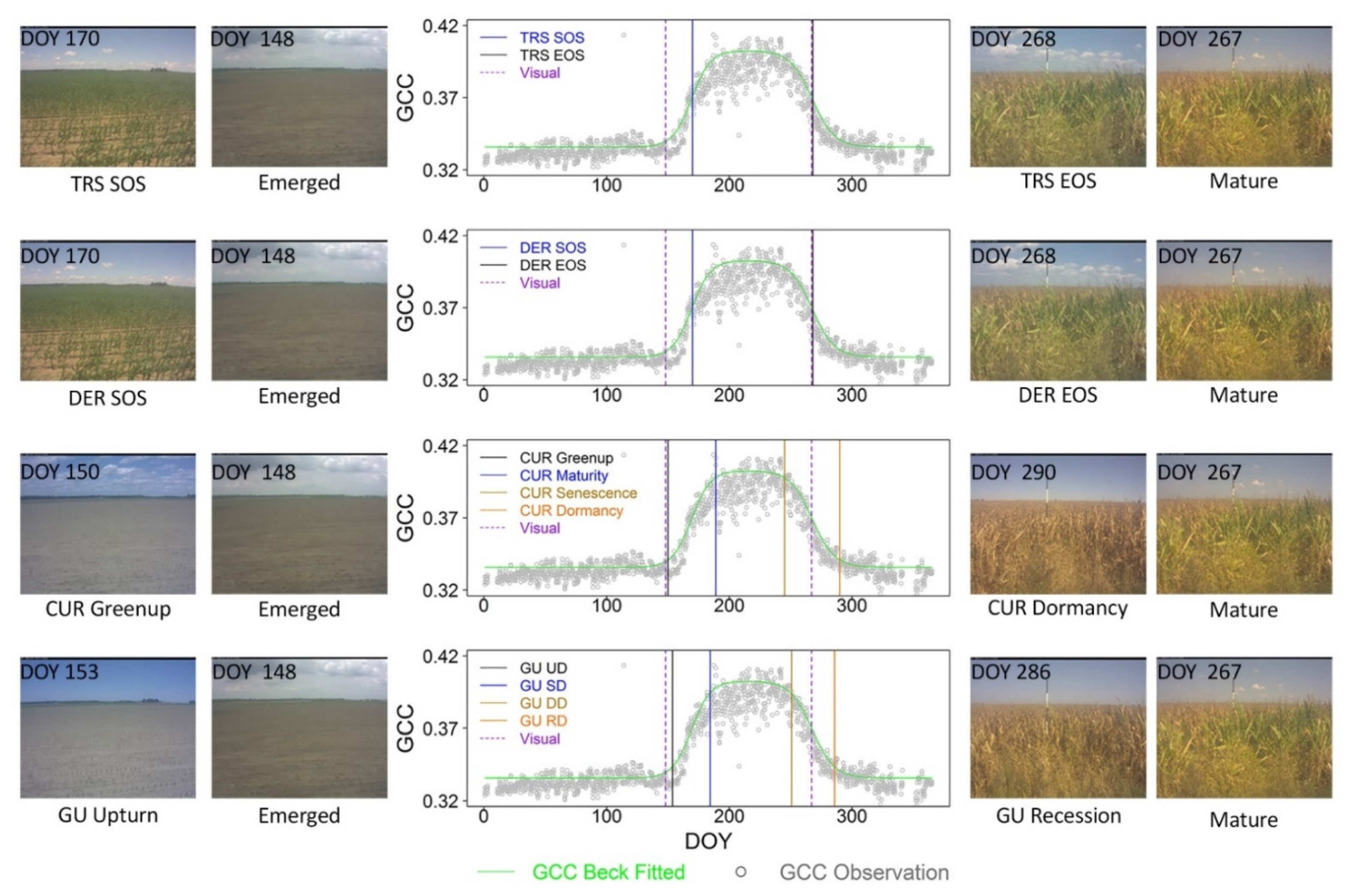
3.1. Fine-Scale Sensor-Based Crop Phenological Characterization

The fine-scale sensor-derived crop phenological characterizations facilitated direct comparisons with visually observed phenological events. With the corn site in the University of Illinois Energy Farm in 2017 as an example, the Beck phenological model fitted to GCC observations was shown in Figure 4. The weighting scheme in Beck diminished the impacts of negatively biased values. The RMSE of the Beck fitting was about 0.01.
At this site, the crop emergence date through the visual observation was about the day of the year (DOY) 148 in 2017, with the consideration of a series of preceding and succeeding PhenoCam photos. The TRS- and DER-based SOS measures were about DOY 170 when the corn had developed several leaves on the ground. The CUR-based Greenup and Maturity estimates were about DOY 150 and DOY 189, respectively. As for the Gu-based method, the UD and SD phenological transition dates were about DOY 153 and DOY 184, respectively. Among the PhenoCam-retrieved phenological characteristics, the CUR-based Greenup and Gu-based UD measures were closer to the visually observed crop emergence date. The corresponding PhenoCam photos exhibited comparable crop status and landscape patterns upon comparison to the photo of crop emergence (Figure 4). The CUR-based Maturity and Gu-based SD estimates, on the other hand, approached the end of the corn vegetative stage when most of the plant leaves were developed.
The crop maturity date by the visual comparison of a series of PhenoCam photos was about DOY 267 when about 50% of corn leaves turned yellow. Among the phenological transition date estimates, the TRS- and DER-based EOS estimates were about DOY 268, of which the crop growth status was comparable to the visually observed one. The CUR-based Senescence and Gu-derived DD dates were about DOY 245 and DOY 250, respectively. During these time periods, the crop was in the reproductive stage with the leave color starting to turn yellow. The CUR-based Dormancy and Gu-derived RD estimates were around DOY 290 and DOY 285, respectively. The corn was ready to be harvested at that time.
The PlanetScope imagery was also analyzed for this specific site-year (Figure 5). About 80 PlanetScope images over the course of the year were downloaded and pre-processed. The Beck phenological model was fitted to pre-processed NDVI observations with the RMSE being 0.016. The phenological characteristics were also estimated to be compared with visually observed crop emergence and maturity dates. Similar to PhenoCam-derived measures, the CUR-based Greenup (DOY 154) and Gu-based UD (DOY 158) estimates were more aligned with the visually observed crop emergence date (DOY 148), upon comparison with TRS- and DER-based SOS estimates (about DOY 173). The TRS- and DER-based EOS estimates (about DOY 262) had better agreement with the visually observed crop maturity date (DOY 267), compared to the CUR-based Dormancy (DOY 291) and Gu-derived RD (DOY 287) estimates. The consistency between the PhenoCam and PlanetScope estimates indicated the potential of interpreting the fine-scale sensor-derived phenological characteristics in the context of visually observed crop phenological events. Given the characteristic positions of estimated transition dates, the visually observed crop emergence date would be compared with TRS-based SOS, DER-based SOS, CUR-based Greenup, and Gu-based UD in subsequent sections. The visually observed crop maturity date would be compared to TRS-based EOS, DER-based EOS, CUR-based Dormancy, and Gu-based RD measures.

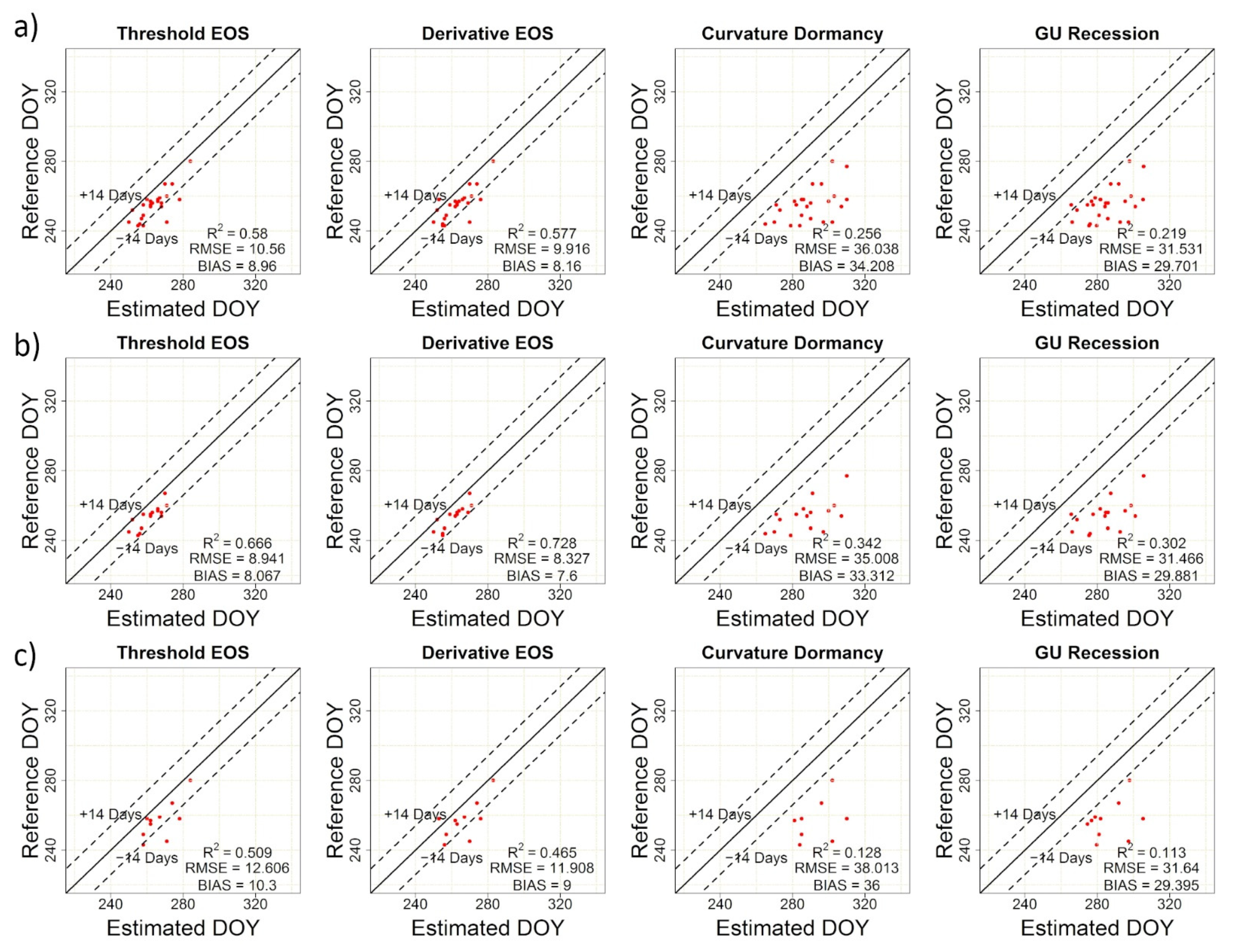
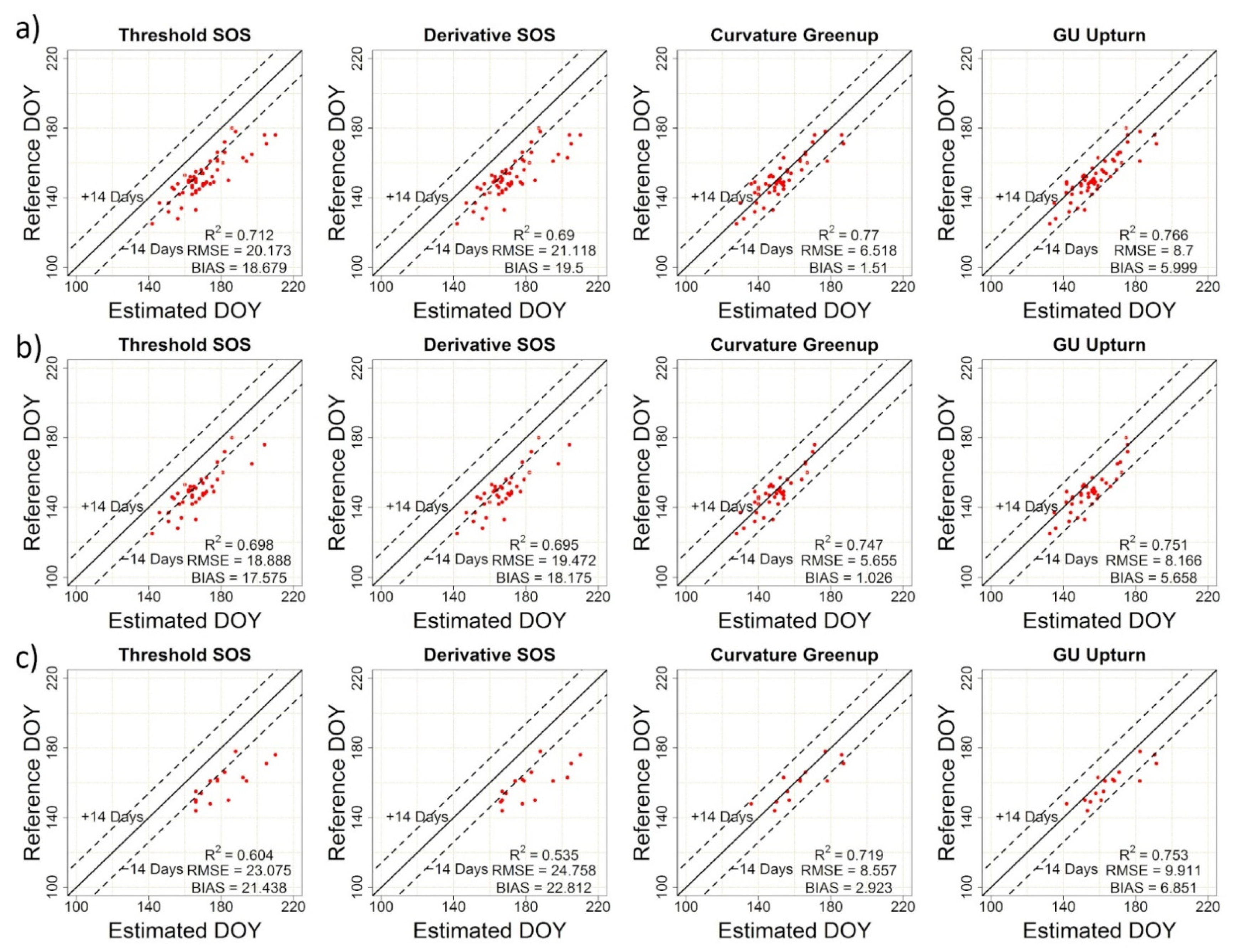
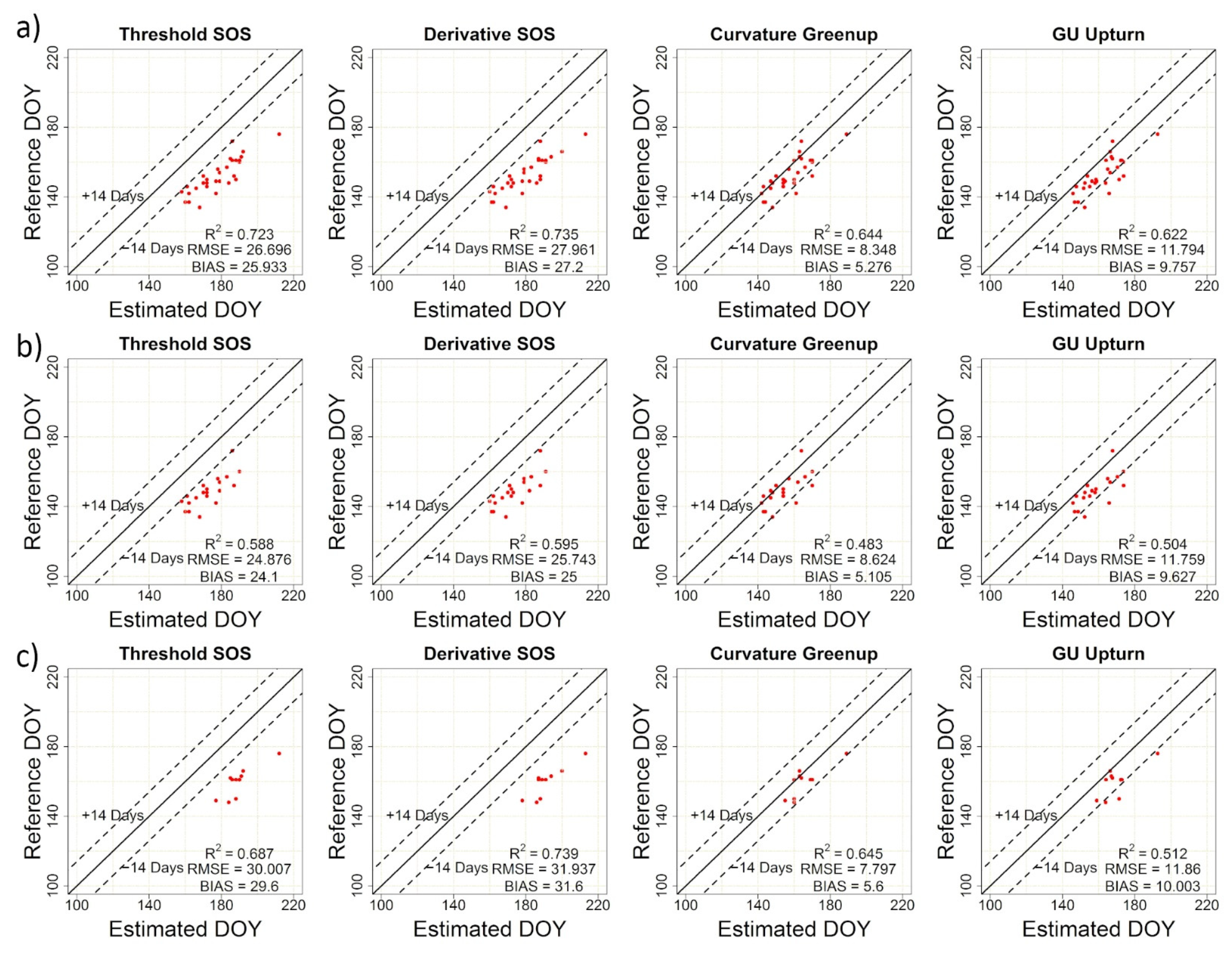
3.2. Concordance between Near-Surface Phenology and Visual Assessment

The 57 PhenoCam site-year photos were visually interpreted via a consistent protocol. The crop emergence dates ranged from DOY 125 to 180 (corn: DOY 125 to 180; soybean: DOY 144 to 178). The crop maturity dates ranged from DOY 242 to 304 (corn: DOY 242 to 304; soybean: DOY 243 to 280). Among all the transition metrics, the CUR-based Greenup and Gu-based UD estimates showed higher degrees of concordance to crop emergence visual observations across sites and years, compared to TRS- and DER-based SOS metrics (Figure 6 and Table 2). Upon comparison to all the corn and soybean emergence observations, the estimated CUR-based Greenup dates were about within one week difference (RMSE = 6.518 days), with most of the comparison points (red dots in Figure 6) distributed along the one-to-one line (bias = 1.51 days). About 77% of the spatiotemporal variance of the emergence observations could be explained by the CUR-based Greenup estimates. Similarly, the Gu-based UD estimates were linearly correlated with the visually observed crop emergence dates, with corresponding R square equal to 0.766, bias being 5.999 days, and RMSE being 8.624 days. The TRS- and DER-based SOS measures, however, were about three weeks delayed from visual observations (about 20 days for both RMSE and bias). With these two metrics, most of the comparison points deviated from the one-to-one line, and the metric dates were much later than the observed ones in PhenoCam photos.
The relationships between PhenoCam and visual assessments were further analyzed for corn and soybean separately. For corn, the average difference between the CUR-based Greenup estimates and visual estimates was within one week (RMSE = 5.655 days), and the corresponding bias was about 1 day. The variation in corn visual emergence across PhenoCam sites and years could be captured by the Greenup estimates with an R square value of 0.747. Similar comparison results were also found in the Gu-based UD estimates (i.e., R square = 0.751, RMSE = 8.166 days, and bias = 5.658 days). The TRS- and DER-based SOS measures had relatively large differences compared to visual observations (about 18 days for both RMSE and bias). Comparable to corn transition date estimates, the soybean CUR-based Greenup and Gu-based UD metrics were about one week different from visually observed emergence dates (RMSE = 8.557 days for Greenup and RMSE = 9.911 days for UD), and those metrics could explain more than 70% of the variation in observed soybean emergence over space and time. The TRS- and DER-based SOS estimates, on the other hand, were more than three weeks away from visual soybean phenological references, with most of the comparison points deviating from the one-to-one line. Both the collective and separate analysis of crop species indicated that the visual change in photos caused by the emergence of crops could be closely linked with CUR- and Gu-based characteristic phenology from the photo-derived GCC seasonal trajectory.
We also compared the phenological transition date retrievals in the downward seasonal trajectory with visually observed crop maturity dates for all the PhenoCam observations. Among all the retrieval metrics, the TRS- and DER-based EOS measures exhibited better congruence with crop maturity visual observations across PhenoCam sites, compared to CUR-based Dormancy and Gu-based RD estimates (Figure 7). The retrieved EOS estimates of all the corn and soybean sites were aligned with visually observed mature dates, with RMSE around 5 days, almost no bias, and R square about 0.75. Comparable EOS-based agreement results were also found in the separate analysis for corn (RMSE around 6 days, bias around 2 days and R square about 0.8) and soybean (RMSE around 5 days, bias around 3 days and R square about 0.83). Those agreement results indicated that visually assessed timing of crops entering the maturity stages with 50% of leaves turning yellow could be approximated by the EOS measures, regardless of crop species considered in this study. Both the collective and separate analysis of corn and soybean sites further showed that the CUR-based Dormancy and Gu-based RD measures were more than two weeks delayed in connecting with crop maturity phenological status. These two measures tended to approach the harvest stage of crops, such as those shown in the 2017 corn site in the University of Illinois Energy Farm (Figure 4).
The collection of agricultural site observations of the PhenoCam network facilitated the understanding of how to crop phenological metrics retrieved from camera canopy-level GCC dynamics related to visually observed phenological events from the same camera photos. The nature and magnitude of covariation between near-surface phenology and visual assessment across sites and years depended on the characteristics of retrieved phenological metrics, with crop emergence more approximated by CUR-based Greenup and Gu-based UD estimates, and crop maturity by TRS- and DER-based EOS estimates (Table 2).

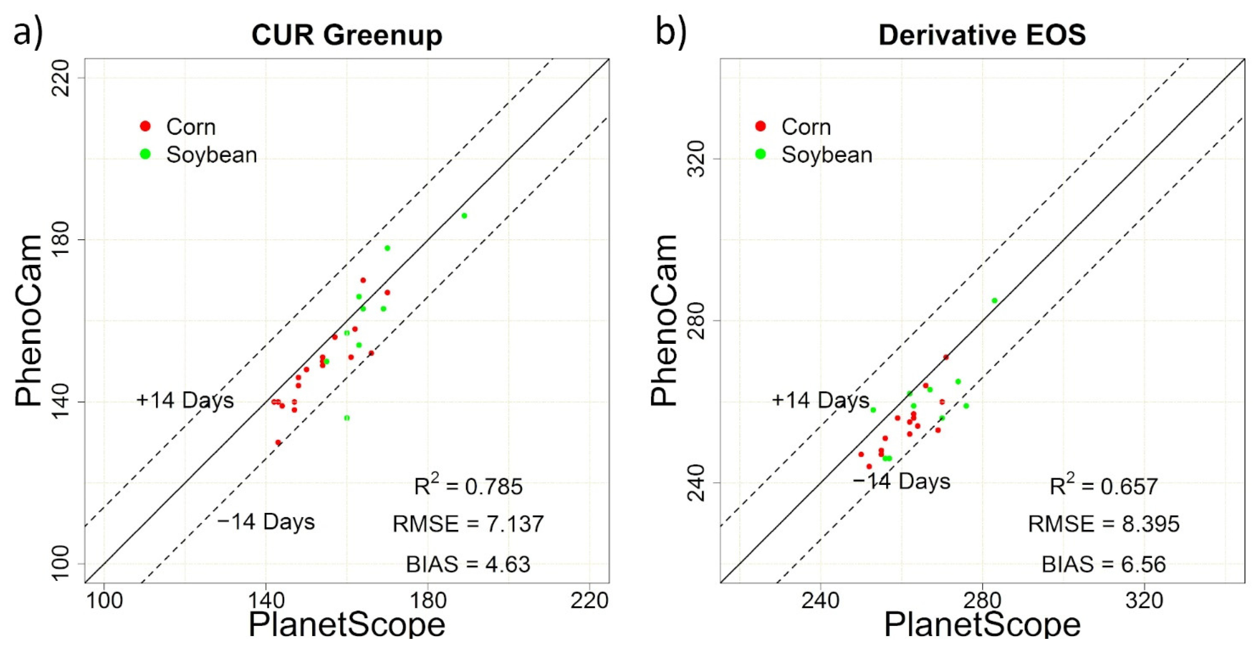
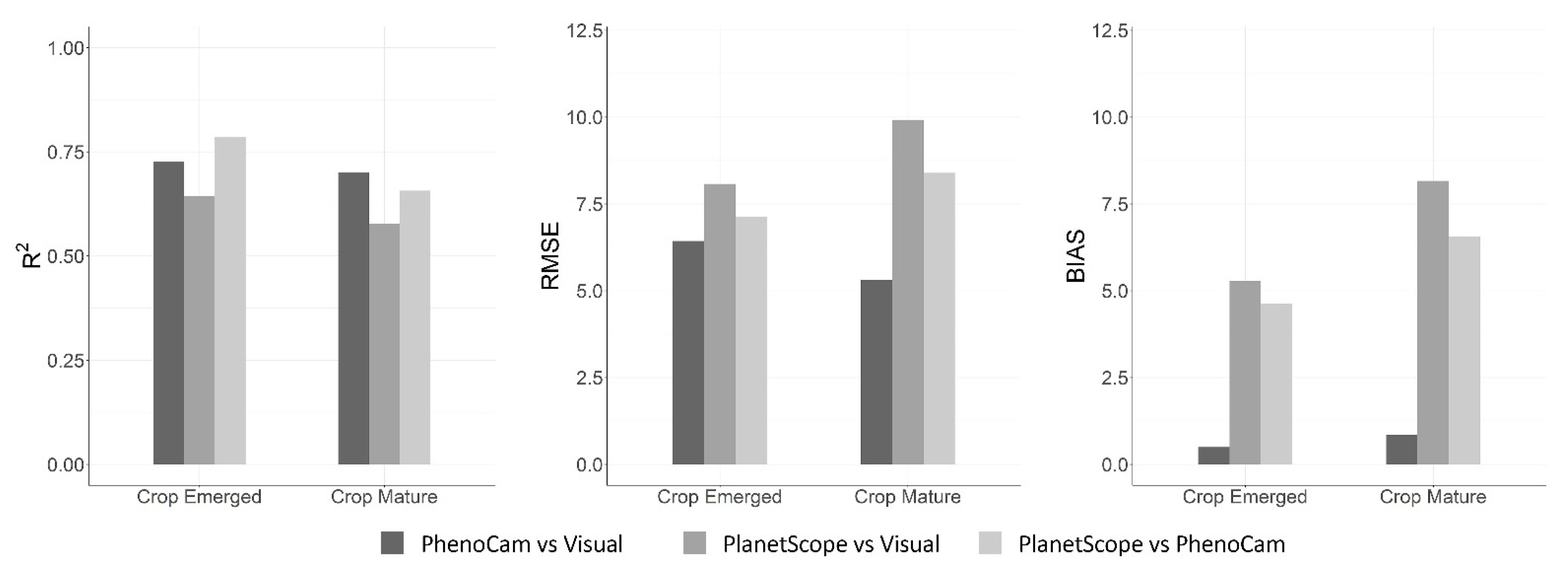
3.3. Concordance among PlanetScope, Near-Surface and Visual Phenology

For the PhenoCam sites that had PlanetScope observations, we further evaluated the degree to which the transition date metrics from the PlanetScope NDVI time series aligned with the visually assessed phenological events from corresponding PhenoCam photos. With the 31 PlanetScope site-year observations, comparable characteristic patterns as those in PhenoCam were found among the transition date metrics, though the PlanetScope-based measures tended to be positively biased with delayed estimations of visually observed phenological events. As for crop emergence, the CUR-based Greenup and Gu-based UD estimates showed better alignment with visual assessments compared to TRS- and DER-based SOS measures (Figure 8). The RMSEs and biases ranged from 1–2 weeks (for Greenup and UD metrics) to 3–4 weeks (for SOS metrics). In particular, the CUR-based Greenup achieved the lowest RMSE (8.348 days) with most of the estimates falling within the one-week interval of emergence observations (bias = 5.276 days) and explained about 65% of the variation in the observed ones. We further conducted the analysis for the corn and soybean sites, respectively. For both species, the CUR-based Greenup estimates attained better agreements with the visual ones (RMSE = 8.624 days and bias = 5.105 days for corn; RMSE = 7.797 days and bias = 5.6 days for soybean) among all the derived transition date metrics.
With regard to crop maturity, the TRS- and DER-based EOS estimates from the PlanetScope time series had about one week difference upon comparison to visual ones in terms of both RMSE and bias (Figure 9). The CUR-based Dormancy and Gu-based RD measures, on the other hand, were positively biased with more than four weeks delayed (bias = 34.208 days for Dormancy and RMSE = 29.701 days for RD). The EOS estimates, with an R square of about 0.58, explained more variance in the maturity observations compared to Dormancy and RD ones (R square of about 0.25). Similar metric patterns were also observed in the separate analysis of the corn and soybean sites, with the crop maturity more approximated by the EOS measures. For corn, the DER-based EOS measure achieved the lowest RMSE (8.327 days) and bias (7.6 days) and explained about 73% of the variance in the corn maturity observations across sites and years. As regards soybean, the RMSE and bias of the DER-based EOS were also the lowest (RMSE = 11.908 days and bias = 9 days) and its R square value was 0.465.
The comparisons conducted for PlanetScope, PhenoCam, and visual phenology indicated the divergent correspondence between transition date metrics and visually observed phenological events. For both PhenoCam and PlanetScope, the CUR-based Greenup exhibited a strong relationship with the photo-based crop emergence observations (Table 2 and Table 3). The DER-based EOS reconciled well with the crop maturity observations. The comparable correspondence patterns between PhenoCam and PlanetScope suggested the potential of connecting fine-scale sensor-derived phenological measures with crop phenological events of biological implications. The CUR-based Greenup and DER-based EOS measures, with their respective good performance, were utilized for the subsequent analysis of the coupled ground and sensor-based crop phenological characterizations.
To further assess the degree to which the PhenoCam-derived metrics aligned with the PlanetScope-based ones, we retrieved the CUR-based Greenup and DER-based EOS measures from both PhenoCam and PlanetScope using all the shared site-year observations (Figure 10). For the CUR-based Greenup, most of the PhenoCam-PlanetScope pairs were distributed along the one-to-one line with the corn in red color and the soybean in green color in Figure 10. About 78.5% of the variance in the PlanetScope-derived Greenup measures was explained by the PhenoCam-based ones. The average measuring difference was 7.137 days using RMSE and 4.63 days using bias. With regard to the DER-based EOS, the PhenoCam-PlanetScope pairs were also aligned along the one-to-one line, with the corresponding R square being 0.657, bias being 6.56 days, and RMSE being 8.395 days. For both measures, the high degree of concordance between PlanetScope and PhenoCam demonstrated the linkage between near-surface and high-resolution satellite-based phenology and indicated the coherence of those fine-scale sensors in retrieving crop phenological characteristics. The RMSEs of about one week between PhenoCam- and PlanetScope-based measures were possibly attributed to the difference in the sensor field of view, viewing angles, and sensor configurations, as well as the difference in crop seasonal dynamics captured by the different vegetation indices.
Finally, we evaluated the concordance among PlanetScope, PhenoCam, and visual phenology with all the shared site-year observations using the CUR-based Greenup and DER-based EOS (Figure 11 and Table 4). Both PhenoCam- and PlanetScope-derived metrics showed a good relationship with crop visual phenological observations. By comparison with visual crop emergence, PhenoCam-derived CUR Greenup estimates were within one week difference (RMSE = 6.43 days), almost no bias, and attained the R square of 0.73. The PlanetScope-based Greenup estimates showed a slightly positive bias (5.28 days), partly due to the use of PhenoCam imagery for visual phenological assessments. Similarly strong correspondence with visual crop maturity was found for both PhenoCam- and PlanetScope-based DER EOS (RMSE = 5.31 days and R square = 0.70 for PhenoCam; RMSE = 9.92 days and R square = 0.58 for PlanetScope), with PlanetScope estimates slightly positive biased (bias = 8.16 days). The congruence among PhenoCam, PlanetScope, and visual crop phenology demonstrated the potential of employing the PhenoCam GCC time series from the RGB imagery to identify critical crop phenological stages, as well as leveraging high-resolution satellite time series for crop phenological detection. The direct comparisons between PlanetScope and visual phenology, along with those between PhenoCam and visual phenology, indicated the linkage of these fine-scale sensors in terms of scale and representation for the coupled ground and sensor-based crop phenological characterizations.

4. Discussion

As two important growth stages, the crop emerged, and mature stages determine the length of the crop growing season and have noted implications for agricultural biogeochemical cycles and crop primary production. We assessed the near-surface PhenoCam and high-resolution PlanetScope imagery in characterizing these two stages of corn and soybean, in comparison with corresponding visual observations. The diverse set of fine-scale sensor-derived phenological metrics had varying agreements with visually observed ones, with RMSE ranging from about 5 days to more than 30 days, indicating the importance of selecting appropriate transition date analysis methods. For both PhenoCam and PlanetScope derived metrics, the CUR-based Greenup and Gu-based UD estimates showed good congruence with visual crop emergence observations (e.g., about one-week RMSE value, small bias, and R square around 0.77 for PhenoCam-Visual emerged comparisons; about 8–11 days RMSE value, 5–9 days bias, and R square around 0.6 for PlanetScope-Visual emerged comparisons). The TRS- and DER-based SOS metrics, on the other hand, deviated from visual crop emergence observations, with RMSE about three weeks for PhenoCam-Visual comparisons and four weeks for PlanetScope-Visual comparisons. The TRS- and DER-based EOS estimates reconciled well with visually observed crop maturity dates, with about 5 days RMSE value, almost no bias, and R square over 0.75 for PhenoCam-Visual mature comparisons, and about 9 days RMSE and bias values with R square around 0.6 for PlanetScope-Visual mature comparisons. Yet the CUR-based Dormancy and Gu-based RD estimates showed a large difference from crop maturity observations. The RMSE and bias of these two estimates were about 3 weeks for PhenoCam-Visual comparisons and more than four weeks for PlanetScope-Visual comparisons. The agreements resonated with our previously developed crop phenological monitoring framework, yet from a novel fine-scale perspective, to shed light on how sensor-derived phenological characteristics could be directly interpreted in the context of visually observed crop phenological stages of physiological significance.
Among the transition date analysis methods, the DER-, CUR-, and Gu-based methods extracted critical crop phenophases based on characteristic points of time series curves (e.g., local maxima/minima in the curvature change rate). By contrast, the TRS-based method identified phenophases via flexibly defined thresholds. In this study, the TRS-based EOS metrics with the 50% threshold aligned well with the visual crop maturity measures. Yet the TRS-based SOS metrics, estimated with the 50% threshold, were much delayed compared to visual crop emergence observations. We further tested a range of threshold values from 5% to 60% with an increment of 5% and found that TRS-based SOS metrics with lower threshold values (e.g., 10%) tended to achieve lower RMSE and Bias values, yet lower R square values for both PhenoCam-Visual emerged comparisons (Figure S1) and PlanetScope-Visual emerged comparisons (Figure S2). With the crop emergence being defined as the timing when the crops were first visible in the PhenoCam photos, the earlier detection dates by lower thresholds of the TRS-based method might be closer to visual emergence dates. Those detection results, however, were also sensitive to noises and fluctuations of time-series curves, leading to lower R square values. For different vegetation indices, crop species, and geographical regions, different thresholds might be needed for the optimized performance of TRS-based methods [17,67,68], which could pose challenges for crop phenology detection from a practical viewpoint.
The establishment of the PhenoCam and other phenology camera-relevant networks has largely facilitated the phenological characterization of individual organisms to landscapes via near-surface remote sensing. With the PhenoCams, we conducted systematic and consistent visual crop phenological interpretations across agricultural sites, as well as retrieved canopy-level phenological metrics through the corresponding GCC time series. The PhenoCam photos, with the sub-daily temporal resolution, enabled the high-quality visual assessment of crop emergence and maturity stages over space and time. For our study sites, the crops exhibited wide ranges of emergence dates (DOY 125 to 180) and maturity dates (DOY 242 to 304) with the visual assessment, due to varying weather, soil, and management conditions of those sites. This visual assessment overcame the labor-intensive issue of field phenological observations, broadened the spatial coverage, and enhanced the connections with pheno-metrics from the GCC-based seasonal trajectory. The pheno-metrics, as shown in this study, could be characterized by different transition date analysis methods. The selection of the analysis methods affected the metric retrieval accuracy (e.g., RMSE, bias, and R square), and thus the correspondence with visually targeted crop phenological stages. The high degree of concordance between CUR-based Greenup and crop emergence (RMSE = 6.43 days, bias = 0.5 days, and R square = 0.73), and between DER-based EOS and crop maturity (RMSE = 5.31 days, bias = 0.85 days, and R square = 0.7), demonstrated the capability of PhenoCams in the fine-scale crop phenological characterizations for precise agricultural management. This could be further enhanced with the continually increasing phenology monitoring network on the global scale. With the unique roles of phenological interpretations and estimations, PhenoCams drastically facilitated the reconciliation of visual- and sensor-assessed crop phenology across broad spatial extents and helped tackle the long-standing challenge of interpreting the sensor-retrieved phenology in the crop growth and physiology-relevant context.
The PlanetScope image time series opened the door for satellite-based crop phenological detection at both high spatial and temporal resolutions and provided unique opportunities to be linked with visual and near-surface crop phenology. Our analysis results indicated that the PlanetScope-derived phenological metrics showed consistent comparison patterns as those from the PhenoCams, with PlanetScope-derived CUR Greenup approaching crop emergence (RMSE = 8.35 days, bias = 5.28 days, and R square = 0.64), and DER EOS for crop maturity (RMSE = 9.92 days, bias = 8.16 days, and R square = 0.58). The good performance of these metrics demonstrated the potential of leveraging the PlanetScope imagery for satellite-based fine-scale phenological retrieval in direct connection with observed crop phenological stages. This connection, in terms of scale and representation, eased the challenge of satellite-based crop phenological validation, which was typically conducted using the satellite imagery of moderate- to coarse- spatial resolutions upon comparison to crop phenological reference at aggregated levels (e.g., district-level or state-level crop progress reports) [19]. It thus facilitated the identification of critical phenological transition dates that were characteristic of crop physiological growth stages using the satellite time series. The PlanetScope time series, with its spatial and temporal resolutions, provided an effective avenue for the fine-scale agricultural seasonal dynamic monitoring and management, though its scientific quality might not be as rigorous as that of other satellites (e.g., MODIS and Landsat) employed for phenological studies [59,69]. Further inter-sensor radiometric calibrations of the PlanetScope imagery to improve the radiometric consistency would be desired in future studies [53]. Yet the calibration procedure usually involved the acquisition of the PlanetScope imagery of a relatively large spatial extent to be compared with corresponding reference imagery typically of coarser spatial resolutions (e.g., acquisition of PlanetScope and MODIS imagery of the same spatial extent), which could be financially prohibitive across the study sites.
The concordance among PlanetScope, PhenoCam, and visual phenology indicated the role of near-surface and high-resolution remote sensing in bridging ground-based phenological observations with conventional satellite-based phenological measures, which were usually derived from the coarse spatial resolution images (e.g., MODIS), and more recently moderate resolution ones (e.g., Harmonized Landsat and Sentinel-2). The scale difference in the conventional satellite-based phenological studies made it challenging to understand how the seasonal trend captured by remote sensing could be reconciled with crop phenological development trajectory. In recent years, the increasing studies of near-surface remote sensing showed the capability of the PhenoCams in tracking the phenological dynamics across the organism-to-ecosystem scales. Besides the PhenoCams, our study also demonstrated the potential of the PlanetScope imagery in facilitating the ground-satellite phenological bridging, which could further benefit the understanding of the effects of scale and representation in phenological retrievals. Yet compared to the PhenoCams, the PlanetScope phenological estimates showed a slightly positive bias for both crop emergence (bias = 4.63 days) and maturity (bias = 6.56 days) in this study. The relatively delayed estimates from the PlanetScope were partially attributed to the difference between the PhenoCam field of view and the associated satellite pixel, and the difference in crop phenological trajectories captured by the different vegetation indices. During the stage of crop emergence, the weak signal of vegetation and associated strong signal of soil background made the capturing of the subtle change of the emergence more difficult in the satellite imagery, compared to near-surface remote sensing. The bias for the crop maturity stage could partially be explained by the heterogeneous status of crop coloration under the camera and satellite field of view. Additionally, the near-surface remote sensing-derived GCC index typically registered the greenness of crop canopies, while the satellite-derived NDVI captured both photosynthetic and structural status. The lag of structural changes in crop growth relative to the changes in its color and pigments might also cause detection bias [70].
In this study, both near-surface PhenoCams and high-resolution PlanetScope imagery showed strong couplings with the observed crop emergence and maturity stages. At fine spatial scales, the coupling relationships also had great potential to be extended to other crop-specific phenological stages (e.g., the silking stage of corn), with the Beck phenological model and appropriately retrieved phenological metrics. Yet as a retroactive approach, the Beck phenological model may have limited ability to conduct near real-time crop phenology monitoring. Compared to natural and managed non-agricultural systems, the crop growth and phenological development in the agricultural systems usually exhibited more diverse and heterogeneous patterns across farm fields. The characterization of these diverse field-level phenological patterns, driven by a combination of climate and farming practices (e.g., sowing date and fertilizer application), could largely be enabled using near-surface and high-resolution satellite imagery. The capability of both imagery in characterizing fine-scale variability in crop phenology had important implications for the efforts toward more sustainable agricultural management and farm-level decision-making, particularly in small-holder agricultural systems. As the influence of weather extremes and farming practices on crop yields varied across phenological stages, such capability facilitated more precise and targeted stage-specific management practices (e.g., fertilizer and harvest scheduling), as well as the improved characterization of yield gap or loss under varying weather conditions at the field to sub-field levels.

5. Conclusions

In this study, we assessed the near-surface PhenoCam and high-resolution PlanetScope time series in characterizing two critical crop phenological stages for a range of agricultural sites across the US. Among the transition date analysis methods, the CUR-based Greenup and Gu-based UD estimates from both PhenoCam and PlanetScope imagery showed good congruence with the visually observed crop emergence stage. The TRS- and DER-based EOS estimates reconciled well with visual crop maturity observations. The concordance among PlanetScope, PhenoCam, and visual phenology demonstrated the potential to interpret the fine-scale sensor-derived phenological characteristics in the context of physiologically well-characterized crop phenological events. This concordance could further facilitate the use of both fine-scale sensors in calibrating and validating phenological models, understanding the relationships between canopy phenology and agroecosystem processes (e.g., gross primary production and carbon-nutrient-water cycling), as well as paving the way to develop formal protocols for bridging ground-satellite phenological characterization. Overall, the intercomparison analysis in this study should increase our capability in retrieving the fine-scale phenological characteristics tied closely to the tangible crop growth stages on the ground and support an improved understanding of global agricultural production, particularly in heterogeneous and small-holder agricultural systems.

Supplementary Materials

The following supporting information can be downloaded at: https://www.mdpi.com/article/10.3390/rs14091957/s1, Figure S1: The accuracy statistics of comparisons between the PhenoCam GCC-based TRS-SOS and the visually observed emergence under different thresholds for the shared corn and soybean sites. Figure S2: The accuracy statistics of comparisons between the PlanetScope NDVI-based TRS-SOS and the visually observed emergence under different thresholds for the shared corn and soybean sites.

Author Contributions

Conceptualization, C.D. and G.L.; methodology, C.D. and G.L.; software, G.L.; validation, C.D. and G.L.; formal analysis, C.D. and G.L.; investigation, C.D. and G.L.; resources, C.D.; data curation, G.L.; writing—original draft preparation, C.D.; writing—review and editing, C.D. and G.L.; visualization, G.L.; supervision, C.D.; project administration, C.D.; funding acquisition, C.D. All authors have read and agreed to the published version of the manuscript.

Funding

This research was funded by the National Science Foundation, grant number 2048068, and the National Aeronautics and Space Administration, grant number 80NSSC21K0946.

Data Availability Statement

This study uses the PlanetScope imagery from the Planet Labs under the education and research program (https://www.planet.com/; accessed on 10 June 2021), and the PhenoCam imagery that is publicly available from the North American PhenoCam network (https://phenocam.sr.unh.edu/webcam/; accessed on 15 November 2020).

Acknowledgments

We gratefully acknowledge the North American PhenoCam network for providing the PhenoCam imagery, and the Planet Labs for providing the PlanetScope imagery.

Conflicts of Interest

The authors declare no conflict of interest. The funders had no role in the design of the study; in the collection, analyses, or interpretation of data; in the writing of the manuscript, or in the decision to publish the results.

References

  1. Richardson, A.D.; Andy Black, T.; Ciais, P.; Delbart, N.; Friedl, M.A.; Gobron, N.; Hollinger, D.Y.; Kutsch, W.L.; Longdoz, B.; Luyssaert, S.; et al. Influence of spring and autumn phenological transitions on forest ecosystem productivity. Philos. Trans. R. Soc. B Biol. Sci. 2010, 365, 3227–3246. [Google Scholar] [CrossRef] [PubMed] [Green Version]
  2. Tang, J.; Körner, C.; Muraoka, H.; Piao, S.; Shen, M.; Thackeray, S.J.; Yang, X. Emerging opportunities and challenges in phenology: A review. Ecosphere 2016, 7, e01436. [Google Scholar] [CrossRef] [Green Version]
  3. Piao, S.; Friedlingstein, P.; Ciais, P.; Viovy, N.; Demarty, J. Growing season extension and its impact on terrestrial carbon cycle in the Northern Hemisphere over the past 2 decades. Glob. Biogeochem. Cycles 2007, 21, GB3018. [Google Scholar] [CrossRef]
  4. Morisette, J.T.; Richardson, A.D.; Knapp, A.K.; Fisher, J.I.; Graham, E.A.; Abatzoglou, J.; Wilson, B.E.; Breshears, D.D.; Henebry, G.M.; Hanes, J.M.; et al. Tracking the rhythm of the seasons in the face of global change: Phenological research in the 21st century. Front. Ecol. Environ. 2009, 7, 253–260. [Google Scholar] [CrossRef] [Green Version]
  5. Walther, G.-R.; Post, E.; Convey, P.; Menzel, A.; Parmesan, C.; Beebee, T.J.C.; Fromentin, J.-M.; Hoegh-Guldberg, O.; Bairlein, F. Ecological responses to recent climate change. Nature 2002, 416, 389–395. [Google Scholar] [CrossRef] [PubMed]
  6. Peñuelas, J.; Rutishauser, T.; Filella, I. Phenology Feedbacks on Climate Change. Science 2009, 324, 887–888. [Google Scholar] [CrossRef] [Green Version]
  7. Richardson, A.D.; Keenan, T.F.; Migliavacca, M.; Ryu, Y.; Sonnentag, O.; Toomey, M. Climate change, phenology, and phenological control of vegetation feedbacks to the climate system. Agric. For. Meteorol. 2013, 169, 156–173. [Google Scholar] [CrossRef]
  8. Piao, S.; Liu, Q.; Chen, A.; Janssens, I.A.; Fu, Y.; Dai, J.; Liu, L.; Lian, X.; Shen, M.; Zhu, X. Plant phenology and global climate change: Current progresses and challenges. Glob. Chang. Biol. 2019, 25, 1922–1940. [Google Scholar] [CrossRef]
  9. Bolton, D.K.; Friedl, M.A. Forecasting crop yield using remotely sensed vegetation indices and crop phenology metrics. Agric. For. Meteorol. 2013, 173, 74–84. [Google Scholar] [CrossRef]
  10. Sakamoto, T.; Gitelson, A.A.; Arkebauer, T.J. MODIS-based corn grain yield estimation model incorporating crop phenology information. Remote Sens. Environ. 2013, 131, 215–231. [Google Scholar] [CrossRef]
  11. Lokupitiya, E.; Denning, S.; Paustian, K.; Baker, I.; Schaefer, K.; Verma, S.; Meyers, T.; Bernacchi, C.J.; Suyker, A.; Fischer, M. Incorporation of crop phenology in Simple Biosphere Model (SiBcrop) to improve land-atmosphere carbon exchanges from croplands. Biogeosciences 2009, 6, 969–986. [Google Scholar] [CrossRef] [Green Version]
  12. Hickman, J.; Shroyer, J. Corn Production Handbook; Publication C: Manhattan, KS, USA, 1994. [Google Scholar]
  13. Lobell, D.B.; Hammer, G.L.; McLean, G.; Messina, C.; Roberts, M.J.; Schlenker, W. The critical role of extreme heat for maize production in the United States. Nat. Clim. Chang. 2013, 3, 497–501. [Google Scholar] [CrossRef]
  14. Lobell, D.B.; Roberts, M.J.; Schlenker, W.; Braun, N.; Little, B.B.; Rejesus, R.M.; Hammer, G.L. Greater Sensitivity to Drought Accompanies Maize Yield Increase in the U.S. Midwest. Science 2014, 344, 516–519. [Google Scholar] [CrossRef] [PubMed]
  15. Lobell, D.B.; Schlenker, W.; Costa-Roberts, J. Climate Trends and Global Crop Production Since 1980. Science 2011, 333, 616–620. [Google Scholar] [CrossRef] [Green Version]
  16. Schlenker, W.; Roberts, M.J. Nonlinear temperature effects indicate severe damages to U.S. crop yields under climate change. Proc. Natl. Acad. Sci. USA 2009, 106, 15594–15598. [Google Scholar] [CrossRef] [Green Version]
  17. Gao, F.; Anderson, M.C.; Zhang, X.; Yang, Z.; Alfieri, J.G.; Kustas, W.P.; Mueller, R.; Johnson, D.M.; Prueger, J.H. Toward mapping crop progress at field scales through fusion of Landsat and MODIS imagery. Remote Sens. Environ. 2017, 188, 9–25. [Google Scholar] [CrossRef] [Green Version]
  18. Diao, C.; Yang, Z.; Gao, F.; Zhang, X.; Yang, Z. Hybrid phenology matching model for robust crop phenological retrieval. ISPRS J. Photogramm. Remote Sens. 2021, 181, 308–326. [Google Scholar] [CrossRef]
  19. Diao, C. Remote sensing phenological monitoring framework to characterize corn and soybean physiological growing stages. Remote Sens. Environ. 2020, 248, 111960. [Google Scholar] [CrossRef]
  20. Wardlow, B.D.; Kastens, J.H.; Egbert, S.L. Using USDA Crop Progress Data for the Evaluation of Greenup Onset Date Calculated from MODIS 250-Meter Data. Photogramm. Eng. Remote Sens. 2006, 72, 1225–1234. [Google Scholar] [CrossRef] [Green Version]
  21. Gao, F.; Anderson, M.C.; Johnson, D.M.; Seffrin, R.; Wardlow, B.; Suyker, A.; Diao, C.; Browning, D.M. Towards Routine Mapping of Crop Emergence within the Season Using the Harmonized Landsat and Sentinel-2 Dataset. Remote Sens. 2021, 13, 5074. [Google Scholar] [CrossRef]
  22. Zeng, L.; Wardlow, B.D.; Xiang, D.; Hu, S.; Li, D. A review of vegetation phenological metrics extraction using time-series, multispectral satellite data. Remote Sens. Environ. 2020, 237, 111511. [Google Scholar] [CrossRef]
  23. Jönsson, P.; Eklundh, L. TIMESAT—A program for analyzing time-series of satellite sensor data. Comput. Geosci. 2004, 30, 833–845. [Google Scholar] [CrossRef] [Green Version]
  24. Zhang, X.; Friedl, M.A.; Schaaf, C.B.; Strahler, A.H.; Hodges, J.C.F.; Gao, F.; Reed, B.C.; Huete, A. Monitoring vegetation phenology using MODIS. Remote Sens. Environ. 2003, 84, 471–475. [Google Scholar] [CrossRef]
  25. Sakamoto, T.; Yokozawa, M.; Toritani, H.; Shibayama, M.; Ishitsuka, N.; Ohno, H. A crop phenology detection method using time-series MODIS data. Remote Sens. Environ. 2005, 96, 366–374. [Google Scholar] [CrossRef]
  26. Diao, C.; Wang, L. Development of an invasive species distribution model with fine-resolution remote sensing. Int. J. Appl. Earth Obs. Geoinf. 2014, 30, 65–75. [Google Scholar] [CrossRef]
  27. Brown, M.E.; de Beurs, K.M. Evaluation of multi-sensor semi-arid crop season parameters based on NDVI and rainfall. Remote Sens. Environ. 2008, 112, 2261–2271. [Google Scholar] [CrossRef]
  28. Diao, C. Innovative pheno-network model in estimating crop phenological stages with satellite time series. ISPRS J. Photogramm. Remote Sens. 2019, 153, 96–109. [Google Scholar] [CrossRef]
  29. White, M.A.; Thornton, P.E.; Running, S.W. A continental phenology model for monitoring vegetation responses to interannual climatic variability. Glob. Biogeochem. Cycles 1997, 11, 217–234. [Google Scholar] [CrossRef]
  30. Diao, C. Complex network-based time series remote sensing model in monitoring the fall foliage transition date for peak coloration. Remote Sens. Environ. 2019, 229, 179–192. [Google Scholar] [CrossRef]
  31. Reed, B.C.; Brown, J.F.; VanderZee, D.; Loveland, T.R.; Merchant, J.W.; Ohlen, D.O. Measuring phenological variability from satellite imagery. J. Veg. Sci. 1994, 5, 703–714. [Google Scholar] [CrossRef]
  32. Gao, F.; Anderson, M.; Daughtry, C.; Karnieli, A.; Hively, D.; Kustas, W. A within-season approach for detecting early growth stages in corn and soybean using high temporal and spatial resolution imagery. Remote Sens. Environ. 2020, 242, 111752. [Google Scholar] [CrossRef]
  33. White, M.A.; De Beurs, K.M.; Didan, K.; Inouye, D.W.; Richardson, A.D.; Jensen, O.P.; O’keefe, J.; Zhang, G.; Nemani, R.R.; Van Leeuwen, W.J.D.; et al. Intercomparison, interpretation, and assessment of spring phenology in North America estimated from remote sensing for 1982–2006. Glob. Chang. Biol. 2009, 15, 2335–2359. [Google Scholar] [CrossRef]
  34. Richardson, A.D. Tracking seasonal rhythms of plants in diverse ecosystems with digital camera imagery. New Phytol. 2019, 222, 1742–1750. [Google Scholar] [CrossRef] [PubMed] [Green Version]
  35. Klosterman, S.T.; Hufkens, K.; Gray, J.M.; Melaas, E.; Sonnentag, O.; Lavine, I.; Mitchell, L.; Norman, R.; Friedl, M.A.; Richardson, A.D. Evaluating remote sensing of deciduous forest phenology at multiple spatial scales using PhenoCam imagery. Biogeosciences 2014, 11, 4305–4320. [Google Scholar] [CrossRef] [Green Version]
  36. Klosterman, S.; Richardson, A.D. Observing Spring and Fall Phenology in a Deciduous Forest with Aerial Drone Imagery. Sensors 2017, 17, 2852. [Google Scholar] [CrossRef] [Green Version]
  37. Richardson, A.D.; Hufkens, K.; Milliman, T.; Frolking, S. Intercomparison of phenological transition dates derived from the PhenoCam Dataset V1.0 and MODIS satellite remote sensing. Sci. Rep. 2018, 8, 5679. [Google Scholar] [CrossRef] [Green Version]
  38. Richardson, A.D.; Hufkens, K.; Milliman, T.; Aubrecht, D.M.; Chen, M.; Gray, J.M.; Johnston, M.R.; Keenan, T.F.; Klosterman, S.T.; Kosmala, M.; et al. Tracking vegetation phenology across diverse North American biomes using PhenoCam imagery. Sci. Data 2018, 5, 180028. [Google Scholar] [CrossRef]
  39. Brown, T.B.; Hultine, K.R.; Steltzer, H.; Denny, E.G.; Denslow, M.W.; Granados, J.; Henderson, S.; Moore, D.; Nagai, S.; SanClements, M.; et al. Using phenocams to monitor our changing Earth: Toward a global phenocam network. Front. Ecol. Environ. 2016, 14, 84–93. [Google Scholar] [CrossRef] [Green Version]
  40. Wingate, L.; Ogée, J.; Cremonese, E.; Filippa, G.; Mizunuma, T.; Migliavacca, M.; Moisy, C.; Wilkinson, M.; Moureaux, C.; Wohlfahrt, G.; et al. Interpreting canopy development and physiology using a European phenology camera network at flux sites. Biogeosciences 2015, 12, 5995–6015. [Google Scholar] [CrossRef] [Green Version]
  41. Nasahara, K.N.; Nagai, S. Review: Development of an in situ observation network for terrestrial ecological remote sensing: The Phenological Eyes Network (PEN). Ecol. Res. 2015, 30, 211–223. [Google Scholar] [CrossRef]
  42. Moore, C.E.; Brown, T.; Keenan, T.F.; Duursma, R.A.; van Dijk, A.I.J.M.; Beringer, J.; Culvenor, D.; Evans, B.; Huete, A.; Hutley, L.B.; et al. Reviews and syntheses: Australian vegetation phenology: New insights from satellite remote sensing and digital repeat photography. Biogeosciences 2016, 13, 5085–5102. [Google Scholar] [CrossRef] [Green Version]
  43. Richardson, A.D.; Jenkins, J.P.; Braswell, B.H.; Hollinger, D.Y.; Ollinger, S.V.; Smith, M.-L. Use of digital webcam images to track spring green-up in a deciduous broadleaf forest. Oecologia 2007, 152, 323–334. [Google Scholar] [CrossRef] [PubMed]
  44. Sonnentag, O.; Hufkens, K.; Teshera-Sterne, C.; Young, A.M.; Friedl, M.; Braswell, B.H.; Milliman, T.; O’Keefe, J.; Richardson, A.D. Digital repeat photography for phenological research in forest ecosystems. Agric. For. Meteorol. 2012, 152, 159–177. [Google Scholar] [CrossRef]
  45. Keenan, T.F.; Darby, B.; Felts, E.; Sonnentag, O.; Friedl, M.A.; Hufkens, K.; O’Keefe, J.; Klosterman, S.; Munger, J.W.; Toomey, M.; et al. Tracking forest phenology and seasonal physiology using digital repeat photography: A critical assessment. Ecol. Appl. 2014, 24, 1478–1489. [Google Scholar] [CrossRef] [PubMed] [Green Version]
  46. Hufkens, K.; Friedl, M.; Sonnentag, O.; Braswell, B.H.; Milliman, T.; Richardson, A.D. Linking near-surface and satellite remote sensing measurements of deciduous broadleaf forest phenology. Remote Sens. Environ. 2012, 117, 307–321. [Google Scholar] [CrossRef]
  47. Baumann, M.; Ozdogan, M.; Richardson, A.D.; Radeloff, V.C. Phenology from Landsat when data is scarce: Using MODIS and Dynamic Time-Warping to combine multi-year Landsat imagery to derive annual phenology curves. Int. J. Appl. Earth Obs. Geoinf. 2017, 54, 72–83. [Google Scholar] [CrossRef]
  48. Melaas, E.K.; Sulla-Menashe, D.; Gray, J.M.; Black, T.A.; Morin, T.H.; Richardson, A.D.; Friedl, M.A. Multisite analysis of land surface phenology in North American temperate and boreal deciduous forests from Landsat. Remote Sens. Environ. 2016, 186, 452–464. [Google Scholar] [CrossRef]
  49. Zhang, X.; Jayavelu, S.; Liu, L.; Friedl, M.A.; Henebry, G.M.; Liu, Y.; Schaaf, C.B.; Richardson, A.D.; Gray, J. Evaluation of land surface phenology from VIIRS data using time series of PhenoCam imagery. Agric. For. Meteorol. 2018, 256–257, 137–149. [Google Scholar] [CrossRef]
  50. Liu, Y.; Hill, M.J.; Zhang, X.; Wang, Z.; Richardson, A.D.; Hufkens, K.; Filippa, G.; Baldocchi, D.D.; Ma, S.; Verfaillie, J.; et al. Using data from Landsat, MODIS, VIIRS and PhenoCams to monitor the phenology of California oak/grass savanna and open grassland across spatial scales. Agric. For. Meteorol. 2017, 237–238, 311–325. [Google Scholar] [CrossRef]
  51. Browning, D.M.; Karl, J.W.; Morin, D.; Richardson, A.D.; Tweedie, C.E. Phenocams Bridge the Gap between Field and Satellite Observations in an Arid Grassland Ecosystem. Remote Sens. 2017, 9, 1071. [Google Scholar] [CrossRef] [Green Version]
  52. Foster, C.; Mason, J.; Vittaldev, V.; Leung, L.; Beukelaers, V.; Stepan, L.; Zimmerman, R. Constellation Phasing with Differential Drag on Planet Labs Satellites. J. Spacecr. Rocket. 2018, 55, 473–483. [Google Scholar] [CrossRef]
  53. Houborg, R.; McCabe, M.F. A Cubesat enabled Spatio-Temporal Enhancement Method (CESTEM) utilizing Planet, Landsat and MODIS data. Remote Sens. Environ. 2018, 209, 211–226. [Google Scholar] [CrossRef]
  54. Houborg, R.; McCabe, M.F. High-Resolution NDVI from Planet’s Constellation of Earth Observing Nano-Satellites: A New Data Source for Precision Agriculture. Remote Sens. 2016, 8, 768. [Google Scholar] [CrossRef] [Green Version]
  55. Houborg, R.; McCabe, M.F. Daily Retrieval of NDVI and LAI at 3 m Resolution via the Fusion of CubeSat, Landsat, and MODIS Data. Remote Sens. 2018, 10, 890. [Google Scholar] [CrossRef] [Green Version]
  56. Sadeh, Y.; Zhu, X.; Dunkerley, D.; Walker, J.P.; Zhang, Y.; Rozenstein, O.; Manivasagam, V.S.; Chenu, K. Fusion of Sentinel-2 and PlanetScope time-series data into daily 3 m surface reflectance and wheat LAI monitoring. Int. J. Appl. Earth Obs. Geoinf. 2021, 96, 102260. [Google Scholar] [CrossRef]
  57. Wu, S.; Wang, J.; Yan, Z.; Song, G.; Chen, Y.; Ma, Q.; Deng, M.; Wu, Y.; Zhao, Y.; Guo, Z.; et al. Monitoring tree-crown scale autumn leaf phenology in a temperate forest with an integration of PlanetScope and drone remote sensing observations. ISPRS J. Photogramm. Remote Sens. 2021, 171, 36–48. [Google Scholar] [CrossRef]
  58. Wang, J.; Yang, D.; Detto, M.; Nelson, B.W.; Chen, M.; Guan, K.; Wu, S.; Yan, Z.; Wu, J. Multi-scale integration of satellite remote sensing improves characterization of dry-season green-up in an Amazon tropical evergreen forest. Remote Sens. Environ. 2020, 246, 111865. [Google Scholar] [CrossRef]
  59. Cheng, Y.; Vrieling, A.; Fava, F.; Meroni, M.; Marshall, M.; Gachoki, S. Phenology of short vegetation cycles in a Kenyan rangeland from PlanetScope and Sentinel-2. Remote Sens. Environ. 2020, 248, 112004. [Google Scholar] [CrossRef]
  60. Dixon, D.J.; Callow, J.N.; Duncan, J.M.A.; Setterfield, S.A.; Pauli, N. Satellite prediction of forest flowering phenology. Remote Sens. Environ. 2021, 255, 112197. [Google Scholar] [CrossRef]
  61. Sadeh, Y.; Zhu, X.; Chenu, K.; Dunkerley, D. Sowing date detection at the field scale using CubeSats remote sensing. Comput. Electron. Agric. 2019, 157, 568–580. [Google Scholar] [CrossRef]
  62. Myers, E.; Kerekes, J.; Daughtry, C.; Russ, A. Assessing the Impact of Satellite Revisit Rate on Estimation of Corn Phenological Transition Timing through Shape Model Fitting. Remote Sens. 2019, 11, 2558. [Google Scholar] [CrossRef] [Green Version]
  63. Seyednasrollah, B.; Young, A.M.; Hufkens, K.; Milliman, T.; Friedl, M.A.; Frolking, S.; Richardson, A.D. Tracking vegetation phenology across diverse biomes using Version 2.0 of the PhenoCam Dataset. Sci. Data 2019, 6, 222. [Google Scholar] [CrossRef] [PubMed] [Green Version]
  64. Beck, P.S.A.; Atzberger, C.; Høgda, K.A.; Johansen, B.; Skidmore, A.K. Improved monitoring of vegetation dynamics at very high latitudes: A new method using MODIS NDVI. Remote Sens. Environ. 2006, 100, 321–334. [Google Scholar] [CrossRef]
  65. Elmore, A.J.; Guinn, S.M.; Minsley, B.J.; Richardson, A.D. Landscape controls on the timing of spring, autumn, and growing season length in mid-Atlantic forests. Glob. Chang. Biol. 2012, 18, 656–674. [Google Scholar] [CrossRef] [Green Version]
  66. Gu, L.; Post, W.M.; Baldocchi, D.D.; Black, T.A.; Suyker, A.E.; Verma, S.B.; Vesala, T.; Wofsy, S.C. Characterizing the Seasonal Dynamics of Plant Community Photosynthesis Across a Range of Vegetation Types. In Phenology of Ecosystem Processes: Applications in Global Change Research; Noormets, A., Ed.; Springer: New York, NY, USA, 2009; pp. 35–58. [Google Scholar]
  67. Bórnez, K.; Richardson, A.D.; Verger, A.; Descals, A.; Peñuelas, J. Evaluation of VEGETATION and PROBA-V Phenology Using PhenoCam and Eddy Covariance Data. Remote Sens. 2020, 12, 3077. [Google Scholar] [CrossRef]
  68. Huang, X.; Liu, J.; Zhu, W.; Atzberger, C.; Liu, Q. The Optimal Threshold and Vegetation Index Time Series for Retrieving Crop Phenology Based on a Modified Dynamic Threshold Method. Remote Sens. 2019, 11, 2725. [Google Scholar] [CrossRef] [Green Version]
  69. Moon, M.; Richardson, A.D.; Friedl, M.A. Multiscale assessment of land surface phenology from harmonized Landsat 8 and Sentinel-2, PlanetScope, and PhenoCam imagery. Remote Sens. Environ. 2021, 266, 112716. [Google Scholar] [CrossRef]
  70. Hufkens, K.; Melaas, E.K.; Mann, M.L.; Foster, T.; Ceballos, F.; Robles, M.; Kramer, B. Monitoring crop phenology using a smartphone based near-surface remote sensing approach. Agric. For. Meteorol. 2019, 265, 327–337. [Google Scholar] [CrossRef]
Figure 1. The geographic locations of the study sites.
Remotesensing 14 01957 g001
Figure 2. The average number of cloud-free PlanetScope images per month across the study sites. The study sites are denoted using the site letters in Figure 1.
Remotesensing 14 01957 g002
Figure 3. The influence of dormant season vegetation on the PhenoCam GCC time series curves. (a) The dormant season vegetation is before the growing season; (b) The dormant season vegetation is after the growing season. The GCC time series was pre-processed with off-season fluctuations replaced by the median dormant season values.
Remotesensing 14 01957 g003
Figure 4. The PhenoCam GCC observations fitted by the Beck double logistic model for the corn site of the University of Illinois Energy Farm in 2017. With the Beck fitted curve, four phenophase analysis methods (i.e., TRS-based, DER-based, CUR-based, and Gu-based methods) were employed to extract phenological metrics to be compared with corresponding visual observations. For this site-year, the visually observed crop emergence date was DOY 148, and the observed crop maturity date was DOY 267. The PhenoCam photos of the extracted metric and visual observation dates were also shown in this figure.
Remotesensing 14 01957 g004
Figure 5. The PlanetScope NDVI observations fitted by the Beck double logistic model for the corn site of the University of Illinois Energy Farm in 2017. With the Beck fitted curve, four phenophase analysis methods (i.e., TRS-based, DER-based, CUR-based, and Gu-based methods) were employed to extract phenological metrics to be compared with corresponding visual observations. For this site-year, the visually observed crop emergence date was DOY 148, and the observed crop maturity date was DOY 267.
Remotesensing 14 01957 g005
Figure 6. The comparisons between the PhenoCam GCCbased transition date estimates of the greenness rising period and the visually observed emergence for (a) both corn and soybean, (b) corn, and (c) soybean, using the four phenophase analysis methods.
Remotesensing 14 01957 g006
Figure 7. The comparisons between the PhenoCam GCC-based transition date estimates of the greenness falling period and the visually observed maturity for (a) both corn and soybean, (b) corn, and (c) soybean, using the four phenophase analysis methods.
Remotesensing 14 01957 g007
Figure 8. The comparisons between the PlanetScope NDVI-based transition date estimates of the greenness rising period and the visually observed emergence for (a) both corn and soybean, (b) corn, and (c) soybean, using the four phenophase analysis methods.
Remotesensing 14 01957 g008
Figure 9. The comparisons between the PlanetScope NDVI-based transition date estimates of the greenness falling period and the visually observed maturity for (a) both corn and soybean, (b) corn, and (c) soybean, using the four phenophase analysis methods.
Remotesensing 14 01957 g009
Figure 10. The comparisons between the PlanetScope- and PhenoCam-derived phenological metrics, including (a) CUR-based Greenup and (b) DER-based EOS, using all the shared site-year observations.
Remotesensing 14 01957 g010
Figure 11. The comparisons among PlanetScope, PhenoCam, and visual phenology with all the shared site-year observations for crop emergence and maturity stages. The CUR-based Greenup metric was estimated for crop emergence and the DER-based EOS metric was estimated for crop maturity.
Remotesensing 14 01957 g011
Table 1. Overview of the PhenoCam study sites and site characteristics.
Study SiteLatitude (Degree)Longitude (Degree)Elevation (m)Site TypeCamera OrientationYearCrop Type
A: Kingman Farm43.17−70.9390Type INA2017–2018Corn
B: Kellogg Biological Station42.44−85.32288Type I and IINA2016–2019Corn, Soybean
C: USDA-ARS Hawbecker Farm40.66−77.85310Type IN2017–2018Corn
D: Peat SSJ River Delta Bouldin Island38.11−121.54−5Type IWNW2018–2019Corn
E: US-Ne1-3 Maize-Soybean Sites41.16−96.47361Type INA2017–2019Corn, Soybean
F: USDA Economic & Environmental research39.03−76.8441Type IN2018–2019Corn, Soybean
G: Swan Lake Research Farm45.68−95.80370Type INNW2016–2019Corn, Soybean
H: ARS Morris. Minnesota LTAR South Tower45.62−96.13341Type IN2018–2019Corn, Soybean
I: Dryland Cropping System46.76−100.93590Type IN2017–2018Corn, Soybean
J: Rosemount Conventional AG Management Site44.69−93.06283Type IN2017–2019Corn, Soybean
K: University of Illinois Energy Farm40.06−88.20224Type I and IIN2011–2019Corn, Soybean
Table 2. The accuracy statistics of comparisons between the PhenoCam GCC-based transition date estimates and corresponding visual observations for all the corn and soybean sites.
Crop EmergenceCrop Maturity
Phenological MetricRMSE (Days)Bias (Days)R2Phenological MetricRMSE (Days)Bias (Days)R2
TRS-SOS20.1718.680.71TRS-EOS5.87−0.520.77
DER-SOS21.1219.500.69DER-EOS6.02−0.310.75
CUR-Greenup6.521.510.77CUR-Dormancy23.9522.430.66
Gu-UD8.706.000.77Gu-RD19.0316.990.65
Table 3. The accuracy statistics of comparisons between the PlanetScope NDVI-based transition date estimates and corresponding visual interpretations using all the PlanetScope site-year observations.
Crop EmergenceCrop Maturity
Phenological MetricRMSE (Days)Bias (Days)R2Phenological MetricRMSE (Days)Bias (Days)R2
TRS-SOS26.7025.930.72TRS-EOS10.568.960.58
DER-SOS27.9627.200.74DER-EOS9.928.160.58
CUR-Greenup8.355.280.64CUR-Dormancy36.0434.210.26
Gu-UD11.799.760.62Gu-RD31.5329.700.22
Table 4. The accuracy statistics of comparisons among PlanetScope, PhenoCam, and visual phenology with all the shared site-year observations using the CUR-based Greenup for crop emergence and DER-based EOS for crop maturity.
ComparisonCrop EmergenceCrop Maturity
RMSE (Days)Bias (Days)R2RMSE (Days)Bias (Days)R2
PhenoCam vs. Visual6.430.500.735.310.850.70
PlanetScope vs. Visual8.355.280.649.928.160.58
PlanetScope vs. PhenoCam7.144.630.798.406.560.66
Publisher’s Note: MDPI stays neutral with regard to jurisdictional claims in published maps and institutional affiliations.

