Abstract
Ice flow lines are the most dominant feature of ice sheet surfaces. Accurate delineation of basins is a prerequisite for mass balance. We therefore propose a new weight balance-based approach to extract the present most comprehensive ice flow lines and then re-delineate the Antarctic basin on this basis. In our approach, we define three impact factors to represent directional accuracy, smoothness, and physical character. Following this, a weight balance-based method is proposed, in which those factors are integrated via weights, to determine the pointing pixels (points or subpixels of the ice flow line). After that, the ice flow lines are continuously tracked. Finally, Antarctic basins were re-delineated based on it. The results indicate that the derived ice flow lines exhibit a rational ice flow pattern against the DEM and the proposed method remarkably improves the performance of results. Furthermore, compared with the Antarctic IMBIE (Ice sheet Mass Balance Inter-Comparison Exercise) basins, the redivided basins exhibit slight diversity, with differences in area and length of less than 11% and a directional accuracy of less than 1° (covering more than 90% of area). As a result, the redivided basins are beneficial to the investigation of the in-depth mechanism of ice shelf calving and mass balance in the Antarctic.
1. Introduction
Flow-parallel features are among the most dominant characteristics of Antarctic ice sheet surfaces [1,2,3]. They originate from the ice sheet interior and continue into its fringing ice shelves [4,5,6], often even extending hundreds of kilometers in length [5,7]. In the glaciological literature, these flow-parallel features are commonly referred to as “longitudinal surface structures”, “flow lines”, “flow stripes”, “flow bands”, or “streak lines” [5,6,8,9,10,11,12,13]. The mapping and distribution of these ice flow lines reveals widespread, complex ice flow configurations covering entire Antarctic ice sheet surfaces, which would provide reliable evidence for the deciphering and tracking potential ice origins. By continuing to track the ice origin of these flow lines—the analysis of their genesis and evolution—researchers are aided in developing an in-depth understanding of their glaciological importance [5,7].
Fluctuations in the mass of Antarctic ice sheets and ice shelves affect global sea levels and oceanic conditions [14,15], which are of considerable importance to climate change. To date, several techniques have been developed and can be used to estimate the state of the Antarctic ice sheet mass balance [16,17,18,19]. Among them, the difference between the accumulation of snowfall over the interior basins and the amount of ice discharges by glaciers across the grounding line is one practical measure [20,21,22]. In this context, the contribution of each interior basin to the total mass budget would be derived to assess continental ice discharge, which implies the future contribution of Antarctica to sea level rise [23,24,25]. The delineation of drainage basins is a prerequisite for the estimation of the mass balance of the ice sheet [14,21,24], which provides geometric information on the range and area of glacier systems, making the estimation of the mass balance comparable [26]. Rignot and Mouginot delineated the drainage basins of Greenland [27] by using surface topography, velocity structure and ancillary data [28]. Mouginot et al. used ice flow direction and the surface slope direction to delineate the Nioghalvfjerdsfjorden and Zachariæ Isstrøm in northeast Greenland [29]. The method based on DEM and ice flow velocity also applied for the delineation of Antarctic drainage basins [24]. Nevertheless, these methods are insufficiently detailed for delineating drainage basin boundaries, while failing to trace the origin of basin ice flows. Yan Liu et al. and D. Floricioiu added ice flow lines to the DEM and velocity data and used them for the delineation of Antarctic and Greenland ice sheet basins, respectively [6,26]. This indicates that flow lines are very valuable for drainage basin delineation and that basins delineated using flow lines will also be more consistent with ice flow trajectories.
The extraction of ice flow lines has long been a classical problem for research. With the development of remote sensing technology, ice flow lines, as the explicit ice flow pattern of ice discharge by glaciers to Antarctic ice shelves, can be delineated by manual or automated extraction of ice flow directions calculated from DEMs or ice flow features derived from satellite imagery [5,7,8,30,31,32,33,34,35,36,37,38]. However, the ice flow directions derived from a DEM can be generally calculated over nonflat ice sheet surfaces, while the visible ice flow lines on satellite images are usually only distributed in fast flow areas, which are limited in their potential to assist in tracking the comprehensive ice flow features from ice origins to fringing ice shelves. In contrast to DEMs and satellite images, the ice flow velocity map over the Antarctic ice sheet surface is aligned with the present-day ice flow directions, which can reliably represent the current glacial dynamics of the Antarctic ice sheet [6]. D. Floricioiu and Yan Liu et al. automatically extracted ice flow lines using the Greenland and Antarctic velocity datasets respectively [6,26]. However, the formerly used vector calculations to extract the flow lines, which resulted in the origin of the flow lines not being available and the accuracy of the flow line extraction not being measured, while the latter mainly considered the direction of the ice flow lines without the smoothness of the flow lines that could lead to some features such as bare rocks being crossed. Therefore, it is necessary to propose a method to obtain complete and smooth flow lines of the Antarctic from the origins on the ice sheet to the surface of the ice shelves.
Despite the lack of satisfactory explanations of their genesis and evolution, ice flow lines as explicit ice flow patterns in the interior of the Antarctic ice sheet have been successfully used to deduce its past and present history [2,5,39] and to delineate Antarctic basins [24,40]. Hence, our objective in this paper is to continuously track the full range of high-density ice flow lines from their ice origins on the Antarctic ice sheet’s interior and onto fringing ice shelves using the MEaSUREs Phase-Based Antarctica Ice Velocity Map (PAIVM) for the period of 2007–2018 and further achieve the fine delineation of Antarctic basins based on the obtained Antarctic ice flow lines map, which would be the basis of studying Antarctica’s dynamic history and performing mass balance-related analysis. Our contributions in this paper are as follows:
- (1)
- This paper proposes a weight balance-based method that utilizes an ice flow velocity map for the extraction of the most complete, high-density ice flow lines currently available that track the trajectory of ice flow from the origins on the ice sheet into the ice shelves. We innovatively define angular, distance, and velocity differences as impact factors to determine the pointing pixel (point or subpixel of the ice flow line). position, which considers the geometric and physical properties of ice flow lines.
- (2)
- Considering the importance of Antarctic basin systems, the differential flow directions occurring at adjacent basin boundaries from ice flow lines are used as the crucial criterion to achieve the fine delineation of Antarctic basin systems and the collapse event of Amery ice shelf occurred in 2019 as the case study for verification.
The rest of this paper is organized as follows. Section 2 describes the proposed method in detail. Section 3 presents the experimental results and analysis for evaluating the proposed method from quantitative and qualitative perspectives. Section 4 discusses the re-delineation of ice basins as well as qualitative and quantitative assessments of basin results. This paper concludes the proposed method in Section 5.
2. Materials and Methods
In this paper, we propose a weight-balance-based method for extracting ice flow lines using an Antarctic ice flow velocity map. First, three features that determine the position of the pointing pixel are obtained, namely, the angular difference, the distance difference and velocity difference, to represent the directional accuracy, the smoothness, and the physical character, respectively. The weight-balanced method was applied to those influencing factors by weighting. Then, we use the pointing-pixel map combined with the flow velocity map to determine the ice origins. Finally, a complete ice flow line is obtained from the ice origins and the pointing pixel map. The flowchart is shown in Figure 1, and we will describe it in more detail in the following sections.
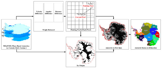
Figure 1.
Flowchart of Antarctic ice flow lines extraction.
2.1. Three Features That Determine the Position of a Pointing Pixel
An ice flow line can be thought of as a polyline consisting of a series of points and segments. The direction of the line segment between two points determines the local direction of the flow line, while the length of the segment determines the smoothness of the flow line. Besides, the flow velocity difference can serve as a physical property to limit the position of the points. Therefore, the most important aspect of determining the ice flow line is determining the position of these points, i.e., finding their pointing points for any point on the ice flow line. As for extracting ice flow lines using ice velocity, we correspond the ice flow lines to the raster data of ice velocity. Then we need to find the pointing pixel (subpixels of the ice flow line) corresponding to the current pixel of the raster data and connect the centers of the pixels. In this section, we will describe in detail the three features that determine the pointing pixel.
2.2. Direction Accuracy of Pointing Pixel
The direction accuracy [6] is an important factor in determining the pointing pixel of the current pixel, which determines the local direction of the ice flow line. The horizontal flow direction calculated from ice velocity map was used to obtain the direction of pointing pixel. However, the flow direction is a vector that cannot be directly used on raster data. Thus, we take the current pixel as the center to establish a Cartesian coordinate system and create an N × N neighborhood. Then, each neighborhood pixel will correspond to an angle which can be calculated by Equation (1). In this paper, it is argued that the closer the angle of a neighborhood pixel is to the flow direction of the current pixel, the higher the directional accuracy. Therefore, we use the angular difference to represent the directional accuracy.
We set the position of the current pixel as , the position of the neighborhood pixel as , and the position of the pointing pixel as , as shown in Figure 2.
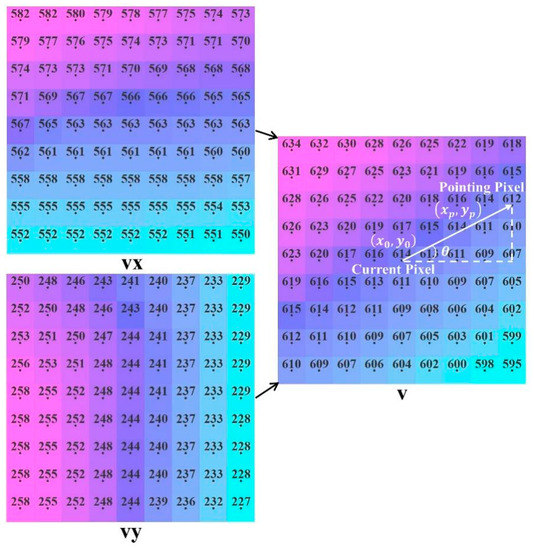
Figure 2.
Diagram of Current pixel and Neighborhood pixel.
Theoretically, when the neighborhood size is infinite, there will exist a pixel in all neighborhood pixels, the angle of which will be infinitely close to the flow direction. Although a larger neighborhood enables a higher directional accuracy, this results in the pointing pixel being too far apart from the current pixel. This means that the ice flow line will not be smooth enough, leading to some small features, such as bare rock or even small islands, being traversed. In addition, it will increase the calculation time needed to find the pointing pixel. Neighborhoods that are too small will result in lower directional accuracy. Therefore, after several tests, it was found that when the neighborhood size was 39 × 39, the minimum difference between any two adjacent pixel angles was less than 0.1 pixels, and the maximum difference was 3 pixels to meet the experimental needs.
2.2.1. Smoothness of the Ice Flow Lines
The distance between the pointing pixel and the current pixel affects the smoothness of the ice flow line, which corresponds to the distance between two neighboring points on the flow line. When corresponding to the neighborhood area, this distance can be calculated by Equation (2).
The shorter the distance between the current pixel and the pointing pixel is, the greater the number of points that make up the ice flow line, and the smoother the ice flow line will be, the longer the distance between the current pixel and the pointing pixel is, the fewer number of points that make up the ice flow line, and the ice flow line will become a polyline.
2.2.2. Velocity Difference of Current Pixel and Pointing Pixel
The velocity difference is the difference between the neighboring pixel velocity and the current pixel velocity. The velocity is a physical property; the distance difference and the angle difference are both geometric properties. The difference in flow velocity between two adjacent points is not too large for an ice flow line, consistent with the ice flow motion. Therefore, the ice flow velocity can also be used as one of the criteria to determine the pointing pixel position. In this paper, it is argued that the smaller the difference between the flow velocity of a neighboring pixel and that of the current pixel, the more likely the neighboring pixel is a pointing pixel. Since the ice flow velocity is a vector, we use the magnitude of the change in flow velocity of the neighboring pixel relative to the current pixel in the x and y directions to calculate the magnitude of velocity difference. Then we use the magnitude of velocity difference to represent the velocity difference of current pixel and pointing pixel.
where is the magnitude of the velocity difference between the velocity of current pixel and neighborhood pixel . The and represent the magnitude of the flow velocity components of pixel n in the x and y directions.
2.3. Weight-Balance Method
The determination of the pointing pixel of each pixel is very important. In existing automatic Antarctic ice flow lines extraction methods, angular difference is only considered [6]. When the neighborhood is larger, it will have higher directional accuracy, but the pointing pixel may be farther away from the current pixel, resulting in poorer smoothness of the ice flow line. The excessive pursuit of directional accuracy will result in small features, such as bare rock or even small islands, being traversed. In addition, the flow velocity is not considered in this process, which is an important physical property for ice flow. According to the ice flow motion, the velocity of the two adjacent points should not differ too much, so we should consider not only the geometric meaning of the flow line but also its physical characteristics. In this paper, it is argued that among the influences of pixel pointing, the flow direction of the current pixel directly affects the local direction of the ice flow line. In contrast, the distance between the current pixel and the pointing pixel affects the distance between the two adjacent points of the ice flow line, and the difference in velocity between the neighboring pixel and the current pixel helps in the identification of a pointing pixel that is more consistent with the ice flow motion. The smaller the angular difference, distance difference, and flow velocity difference is, the better the results.
Weight balancing is a method that allows multiple factors to be considered jointly by weighting, and it satisfies our need to use them simultaneously to determine the pointing pixel, where we need to design the weights of each influencing factor. We consider the angular difference to be the most important of the three influences since it directly affects the directional accuracy of each point of the ice flow. Therefore, the angular difference is designed with a larger weight, while the distance difference and the velocity difference limit the position of each point, with the former determining the smoothness of the flow line and the latter being used to find the point that best matches the physical properties of the ice flow. Consequently, we limit the weight of the angular difference to 1, while the velocity difference and the flow velocity difference are tested at weights , respectively.
In the experiment, the Amery ice shelf basin is selected to test different weights and repeatedly compare the ice flow line generation results. The experimental results show that optimal results can be obtained by the weighting design .
where is the weighted feature corresponding to each neighborhood pixel. is the flow direction of the current pixel, which is provided by the ice velocity map. This paper finds the pixel with the smallest value of among all pixels in the neighborhood range, which is the pointing pixel of the current pixel.
2.4. Determine the Ice Origins
Most of the ice flow lines originate in the interior of the ice sheet [5,31] and outflow from areas of high elevation within the ice sheet into the surrounding ice shelves. The complete ice flow trajectory can be derived through tracing each sub-pixel of the flow line by obtaining the ice origin of the line. However, obtaining these ice origin points is difficult for DEMs and images because the interior of the ice sheet is often terrestrially flat and lacks identifiable ice flow features. Nevertheless, this problem can be solved by using the ice flow velocity datasets and the pointing pixel map obtained above, for which we identify the ice origin points by the following characteristics:
- (1)
- The ice flow velocity at the ice origin velocity is close to 0 m/yr.
- (2)
- The ice origins are not pointed to by any of the pixels.
For the second characteristic, this paper creates a label map. The initial value of each pixel in this label map is 0, which means that no initial pixel has been pointed out. After the method above, the pointing pixel of each pixel in the flow velocity map is determined, and the value of the pointing pixel in the label map is recorded as being 1. At this time, the label map should contain two types of pixels: pixels with a value of 0 that are not pointed to by any pixel, and pixels with a value of 1 that are pointed to. In this way, all the pixels that are not pointed to by the pixel can be obtained. These pixels may include the ice origins and the pixels in space caused by the large interval of ice flow lines. Therefore, this paper continues to obtain the ice origins according to the ice flow velocity map, with velocities less than 3 m/yr. The ice origins are independent of each other and disordered. A complete ice flow line can be extracted from any of the ice origins based on the distribution of pointing pixels.
2.5. Antarctic Ice Flow Lines Map Generation
We extracted the ice flow lines by tracing from the ice origins to the end of the ice shelf into the sea. The tracking process first traverses the ice origins, and then if the ice origin pointing pixel exists, the current pixel and the pointing pixel are connected. The pointing pixel then becomes the current pixel, and its corresponding pointing pixel is found if it exists; therefore, the ice flow line is tracked until the current pixel has no corresponding pointing pixel or reaches the boundary of the experimental area and then focus is shifted to the next ice origin. To prevent dead loops caused by errors in the original data or by the fact that some ice origins are pointing to themselves, the tracking stops when the pixel points to itself. When all the ice origins are traversed, all the ice flow lines are obtained (Figure 3).
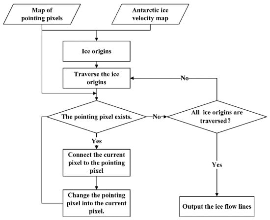
Figure 3.
Flowchart of the Ice flow lines generation.
2.6. Antarctic Basins Delineation Based on Ice Flow Lines Map
Based on the mentioned method, we can produce an Antarctica-scale ice flow line map, which reflects the comprehensive trajectory of the ice flows from their ice origins into fringing ice shelves. In this section, we describe a method for delineating Antarctic basin systems using the derived ice flow lines.
The accurate delineation of Antarctic basin systems is a prerequisite for the investigation of Antarctic mass balance [14,21,24], which calculates the ice material loss from each basin. On the basis of Antarctic basin systems, ice flux across the Antarctic ground line from each Antarctic basin is determined through the generated high-density comprehensive ice flow line map. In our implementation, the re-delineation of Antarctic basins is based on the frequently-used Antarctic IMBIE basins, which are acquired by historical definitions [41], current DEM, and ice velocity data [24]. Compared with the previous DEM-based basin delineation [21], the base data used, i.e., Antarctic IMBIE basins, exhibit better basin delineation results by introducing the surface slope from the TanDEM-X DEM and the flow direction derived by flow velocity with a high flow direction accuracy (error < 2°). Different from the surface slope from the DEM and the flow direction from the flow velocity, the different flow directions at the adjacent basin boundaries from the ice flow lines offer the crucial delineation criterion, which is the key insight behind Antarctic basin re-delineation. To distinguish the ice flow lines from each other, we represent the flow lines with different colors. For adjacent basins, we reclassified the boundaries of adjacent basins by tracing the flow trajectories of flow lines at the boundaries of adjacent basins. In contrast to the boundaries of adjacent basins, we retain and keep the boundaries of ice shelves in Antarctic IMBIE basins since they were based on InSAR-derived grounding lines with high accuracy. As a result, the boundaries of all adjacent basins were redefined to generate the re-delineated Antarctic basin systems [42].
Research manuscripts reporting large datasets that are deposited in a publicly available database should specify where the data have been deposited and provide the relevant accession numbers. If the accession numbers have not yet been obtained at the time of submission, please state that they will be provided during review. They must be provided prior to publication.
Interventionary studies involving animals or humans, and other studies that require ethical approval, must list the authority that provided approval and the corresponding ethical approval code.
3. Experimentation and Analysis
In this section, we first give a brief description of the experimental data used in this paper. Then, we perform both qualitative and quantitative analyses to evaluate the performance of the proposed weight-balance-based ice flow line extraction algorithm. The proposed method is also compared with the classical method of ice flow lines extraction. In our implementation, we take the B-C basin [24] and its fringing Amery ice shelf as a typical case study to investigate the effect of three impact factors in the proposed method on ice flow line extraction and perform a statistical analysis of the density of the derived ice flow lines. Since the Amery ice shelf is the third largest ice shelf in Antarctica and, in recent years, Amery ice shelf collapse events have occasionally occurred, it is of great research interest. As a result, we produced a high-density continent-scale map of Antarctic ice flow lines. Note that since the derived ice flow lines have a very high density, we set an interval between ice origins to achieve the thinning of the ice flow lines for better visualization. The density of the ice flow lines in the figures presented throughout this paper is 1/5 of the original results, except for the ice flow lines display and density calculation for the B-C basin and its fringing Amery ice shelf.
3.1. Experimental Data
For both qualitative and quantitative analysis, the data sources used in this paper are as follows: (1) MEaSUREs Phase-Based Antarctica Ice Velocity Map (PAIVM) [43] for the period from 2007 to 2018, which is available from https://nsidc.org/data/nsidc-0754/versions/1 (accessed on 7 March 2021), has a 10-fold velocity precision (20 cm/year) compared to the prior comprehensive mappings [44] with directions (5°) covering 80% of Antarctica (Figure 4a). The high precision of ice flow velocity in the interior of the Antarctic ice sheet surfaces satisfies our need to extract complete ice flow lines, especially for the purpose of obtaining ice origins. (2) MEaSUREs Antarctic Boundaries for IPY (International Polar Years) 2007–2009 [41,45,46], which is available from https://nsidc.org/data/nsidc-0709/ (accessed on 7 March 2021), provides maps of the Antarctic ice shelves, Antarctic basins, and Antarctic ground lines (as shown in Figure 4b). (3) The auxiliary data consists of Bedmap2 (as shown in Figure 4c) [47], which is available from https://www.bas.ac.uk/project/bedmap-2/#data (accessed on 7 March 2021), and MODIS Mosaic of Antarctica 2008–2009 (MOA2009) Image Map (as shown in Figure 4d) [48], which is available from https://nsidc.org/data/nsidc-0593 (accessed on 7 March 2021), which is primarily used for qualitative comparisons with the proposed method.
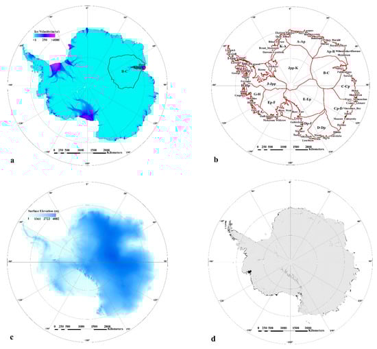
Figure 4.
Overview of experimental data. (a) PAIVM. (b) Antarctic boundaries. (c) Bedmap2 surface elevation. (d) MOA2009.
3.2. Quantitative Assessment of Ice Flow Lines Extraction Results
The key insight behind this paper is that the velocity difference, angular difference, and distance difference between ice flows can affect the position of each point on the ice flow lines. In our implementation, the proposed weight-balance-based method jointly considers these three impact factors to recover the comprehensive ice flow lines from their ice origins. To investigate the roles of three impact factors in the proposed weight balance-based method from quantitative perspectives, in this subsection, we take the B-C basin and its fringing Amery ice shelf as a typical case study. In this paper, the error of the extracted ice flow lines mainly comes from the following two aspects: the error of the experimental data itself, i.e., PAIVM, and the position errors of each point on the ice flow lines. Actually, the error of the former [43] is negligible compared to the latter. Therefore, we focus on the error of the proposed method, which is mainly reflected in the position of each pointing pixel (sub-pixel) of the ice flow line. In the proposed method, converting the vector direction of the flow velocity into a specific pointing pixel of the ice flow line may introduce errors. The neighborhood raster size cannot be set too large because of the constraints on computational efficiency and smoothness and velocity differences of the flow line when finding the pointing pixels. After several experiments to determine the size of the neighborhood, the conversion of the directional vector of velocity into a specific raster position by balancing the angular, distance, and velocity differences with weights results in angular, velocity, and distance differences the sub-pixels of the ice flow line.
Figure 5 shows the distribution of the angular, distance, and velocity differences of the pointing pixels in the B-C basin and the fringing Amery ice shelf (Figure 5a–c), as well as the corresponding cumulative frequency distribution histograms (Figure 5d–f). As shown in Figure 5d, over 90% of the pixels suggest an angular difference of less than (nearly 100% ). Similarly, for distance differences, as shown in Figure 5e, over 95% of the pixel distance differences are less than 10 pixels. Furthermore, for the flow velocity difference (Figure 5f), nearly 90% of the pixels exhibit a flow velocity difference of less than 1 m/yr. Therefore, we can conclude that for most of the B-C basin and its fringing Amery ice shelf, our result indicates a high directional consistency, a high smoothness, and identical physical characteristics. At the same time, considering the spatial distribution of these three impact factors (as shown in Figure 5a–c), we also find that the minimum angular difference, minimum distance difference, and minimum velocity difference are often not satisfied simultaneously. Consequently, the position of the pointing pixel is not determined by a single impact factor, which further verifies the validity of the proposed weight balance-based method.
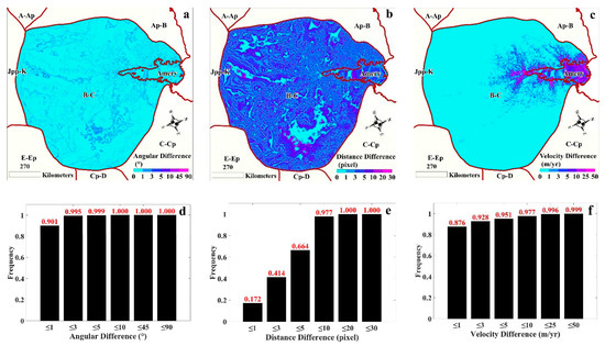
Figure 5.
Spatial distribution of angular, distance, and velocity differences of pointing pixels in the B-C basin and its fringing Amery ice shelf as well as the corresponding cumulative frequency distribution histograms. (a) Spatial distribution of angular difference. (b) Spatial distribution of distance difference. (c) Spatial distribution of velocity difference. (d) Cumulative frequency distribution histogram of angular difference. (e) Cumulative frequency distribution histogram of distance difference. (f) Cumulative frequency distribution histogram of ice flow velocity difference.
In addition to calculating the angular, distance and velocity differences of the pointing pixels in the Amery basin, we also calculated these three differences for the ice flow lines. Considering that the ice flow line is made up of individual subpixels (pointing pixels), the Root Mean Square Error (RMSE) of the angular, distance and velocity differences at each subpixel of the ice flow line were calculated to represent the angular, distance and velocity differences of the ice flow lines. Besides, the maximum values of the angular, distance and velocity differences at each subpixel of the ice flow lines were obtained to represent the maximum values of those differences of the ice flow lines. As can be seen from the Figure 6, for the angular difference, which is a factor of directional accuracy, more than 90% of the pixels have an angular difference of less than 3°; for the distance difference, which is a factor of smoothness, more than 90% of the pixels have a distance difference of less than 10 pixels; and more than 90% of the pixels have a velocity difference of less than 1 m/yr.
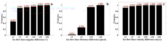
Figure 6.
Cumulative frequency distribution histogram of ice flow lines angular difference, distance difference and velocity difference. (a) Cumulative frequency distribution histogram of ice flow lines angular difference. (b) Cumulative frequency distribution histogram of ice flow lines distance difference. (c) Cumulative frequency distribution histogram of ice flow lines velocity difference.
Furthermore, as can be seen from the Table 1, the maximum values of angular difference, distance difference and flow velocity difference for ice flow lines are less than 5° (for more than 90% of flow lines), less than 10 pixels (for more than 75% of flow lines) and less than 1 m/yr (for more than 90% of flow lines).

Table 1.
The maximum value of the angular difference, distance difference and velocity difference of the ice flow lines.
After that, we calculate and count the total length of each ice flow line in the B-C basin and its fringing Amery ice shelf by accumulating the distances between two consecutive points along the query ice flow line. In the B-C basin, the total number of derived ice flow lines is 1306861, with a tracking capacity of 1589.540 km from their ice origins. As shown in Figure 7a, longer ice flow line lengths mainly flowed through the Amery Ice Shelf, while shorter lengths were mainly found in the interior of the ice sheet and on islands or bare rock outcrops, which is consistent with the findings of previous studies [35].
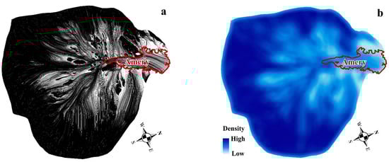
Figure 7.
Ice flow lines and its density of B-C basin and its fringing Amery ice shelf (no thinning of ice flow lines). (a) Ice flow lines. (b) Density of ice flow lines.
In addition to the length, the density of ice flow lines is defined as the total length of longitudinal surface structures falling within a circular supporting neighborhood from each query grid node, divided by the area of the supporting neighborhood. In our implementation, the radius of the supporting neighborhood is set to 100 pixels.
The density distribution of ice flow lines (Figure 7b) shows that the densest distribution of ice flow lines is in the interior ice sheet, which is also the main region of ice origins. On the ice shelf surface, the ice flow lines are distributed in a fan shape, which is also consistent with the glacier dynamics in this region.
3.3. Qualitative Assessment of Ice Flow Lines Extraction Results
To investigate the roles of three impact factors used in the proposed weight balance-based method from qualitative perspectives, in this subsection, we select the middle and front of the Amery ice shelf (marked as cases #1 and #2) to evaluate the ice flow line extraction results derived from the proposed method, the weight balance-based method considering angular difference and distance difference and the method only considering angular difference. Figure 8 shows comparisons of the ice flow line extraction results on the partial Amery ice shelf. As shown in Figure 8a,b,d,e, the results show some crossing issues associated with the derived ice flow lines, some of which even pass-through small islands (as highlighted in blue polygons). In contrast, the proposed method in this paper remarkably improved the results by weighting the velocity difference, angular difference, and distance difference of the evaluated ice flows. Thus, the proposed method in this paper effectively balances the relationship between the three impact factors of ice flow lines to generate smooth and rational ice flow lines.
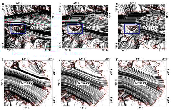
Figure 8.
Comparisons of ice flow line extraction result on the partial Amery ice shelf. The black lines denote the derived ice flow lines, the red lines denote the boundaries of Amery ice shelf. (a) Method only considering angular difference (case #1). (b) Weight-balance-based method considering angular difference and distance difference (case #1). (c) Proposed method (case #1). (d) Method only considering angular difference (case #2). (e) Weight-balance-based method considering angular difference and distance difference (case #2). (f) Proposed method (case #2).
Since our method is a weight-balancing approach that considers angular, distance and flow velocity differences together. To verify that our method does not change the flow direction of the flow lines in areas where there is an abrupt change in flow velocity, such as when an ice stream merges into a fast ice stream, as compared to a method using only angular and distance differences, we chose two such areas (marked as case #3 and #4) in the Amery ice shelf to verify this. In the areas of Figure 9a,b, the black line shows the method in this paper and the white line shows the method using only angular and distance differences. From Figure 9 we can see that the flow direction of the flow line has barely changed.
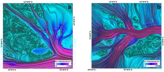
Figure 9.
Comparison of flow lines between the proposed method and the method using only angular and distance differences, the black line shows the method in this paper and the white line shows the method using only angular and distance differences. (a) Comparison of flow lines between the proposed method and the method using only angular and distance differences (case #3). (b) Comparison of flow lines between the proposed method and the method using only angular and distance differences (case #4).
3.4. Comparison of the Proposed Method with Other Flow Lines Extraction Methods
In addition, we compare the results of the proposed method with widely used traditional methods for manual extraction of ice flow lines from DEM and optical remote sensing images [5,9]. In our implementation, the manual extraction of ice flow lines is conducted from Bedmap2 surface elevation and MOA2009 data. To achieve the manual extraction of ice flow lines, the aspect map based on Bedmap2 surface elevation is calculated to exhibit the topographic relief, and the image enhancement method using the most effective histogram equalization [8,38] is carried out on MOA2009 to improve the contrast across the ice surface. Figure 10 demonstrates comparisons of ice flow line extraction on the Amery ice shelf between the proposed method and other Antarctic datasets. The results suggest that the derived ice flow lines exhibit good agreement with most surface longitudinal features on both the Bedmap2 surface elevation and MOA2009 analyses. Compared with the results from both the Bedmap2 surface elevation and MOA2009 analyses, the results with a comprehensive motion trajectory of ice discharge to ice shelf from its ice origins are produced more easily through the proposed method.
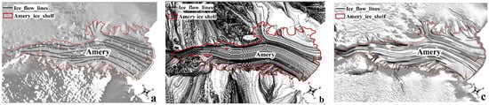
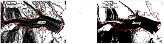
Figure 10.
Comparisons of ice flow lines extraction on Amery ice shelf among the proposed method, other Antarctic data sets and Matlab and Python streamline function. The aspect map and MOA 2009 are used as background in subfigures (a,c), respectively. (a) Ice flow lines from Bedmap2 surface elevation. (b) Ice flow lines by the proposed method. (c) Ice flow lines from MOA2009. (d) Matlab Streamline extraction of ice flow lines. (e) Matlab Streamline extraction of ice flow lines.
For the automatic extraction of ice flow lines, we compared the proposed method with Matlab (https://ww2.mathworks.cn/help/matlab/ref/streamline.html, accessed on 7 January 2021) and Python (https://plotly.com/python/streamline-plots, accessed on 8 January 2021) Streamline extracted function. The Streamline function in Python does not require ice origins to be set to extract flow lines, whereas the Streamline function in Matlab requires ice origins to be provided, thus we use the ice origins from the proposed method as input to the Streamline function in Matlab. A comparison of the results is shown in Figure 10d,e above. The Streamline function in Matlab and Python can also extract ice flow lines as can be seen in Figure 10d,e. However, apart from the problems mentioned above with these two methods, they are based on vectors and therefore cannot evaluate the accuracy of the ice flow lines. In addition to this, as can be seen in the figure, the proposed method is also more complete and smoother than these two methods.
In contrast to the above method of extracting flow lines through vector calculations, the method proposed by Liu Yan et al. which considers directional accuracy to extract ice flow lines using ice flow velocity [6] is comparable. The subpixels of the ice flow lines are located at the center of the raster as in our method. Therefore, it is possible to compare the overall directional accuracy, smoothness, and velocity difference of the flow lines. We use the Amery basin to compare the two methods and part of the results are shown in Figure 8a,d for the flow lines considering only directional accuracy and in Figure 8c,f for the proposed method. As can be seen in the Table 2 below, although the directional accuracy of the flow lines of the proposed method is lower than the accuracy of the flow lines obtained by considering only the directional accuracy, the RMSE of the directional accuracy of more than 90% of the flow lines is less than 3°, which is very close to that of the method considering only the directional accuracy. In addition, the smoothness and angular difference of the flow lines of the proposed method are much higher than those of the direction accuracy-only method.
Table 2.
The cumulative frequencies of angular difference, distance difference and velocity difference for the flow lines of the proposed method compared to the angular difference only method.
Following this, the proposed weight-balance-based ice flow line extraction method is applied to the entire Antarctic ice flow velocity map to produce a high-density continent-scale map of Antarctic ice flow lines. Figure 11 illustrates an overview of the extracted ice flow line map by the proposed method. To verify the relationship between the derived ice flow line map and the Bedmap2 surface elevation data, the derived ice flow line map is overlaid with the Bedmap2 surface elevation data. The red polygon in Figure 11 is the grounding line of Antarctica. As shown in Figure 11, it can be concluded that the ice flows move from the higher inland regions of Antarctica to the fringing ice shelves and continue into the ocean from the front of the ice shelves. The high degree of consistency between the ice flow pattern represented by the derived ice flow line map and the topographic relief further indicates the reliable and robust performance of the proposed weight-balance-based ice flow line extraction method. In addition, the results also demonstrate that the proposed method can continuously trace the comprehensive ice flow line from the highest ice origins in the Antarctic inland to the ice shelf, which is beneficial to the efficient recovery of the entire trajectory of Antarctic ice discharge.
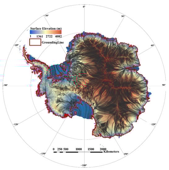
Figure 11.
Overview of the extracted ice flow line map by the proposed method. Bedmap2 elevation data is used as background for better visualization.
4. Discussion
The ice flow lines are considered the explicit ice flow pattern of ice discharged by glaciers to the Antarctic ice shelves. The tracking and recovery of their motion trajectories are beneficial to the analysis of Antarctic glacier dynamics and mass balance calculations. The ice flow velocity map derived from multiphase satellite imagery is aligned with the present-day flow direction, which offers key support for the extraction of ice flow patterns. Therefore, this paper presents a novel weight balance-based method from an ice flow velocity map for extracting high-density comprehensive ice flow lines in Antarctica.
The key insight behind the proposed method is that the velocity difference, angular difference, and distance difference of ice flows can affect the position of each point on the ice flow line. The roles of these three impact factors are investigated during the extraction of ice flow lines. The results suggest higher direction consistency and smoothness (covering nearly 90% of Antarctica), especially on small structurally isolated islands, as well as a tracking capacity of over 1589.540 km from the ice origins. Furthermore, the results from the proposed method have a high agreement with the previous results derived from other Antarctic datasets. In summary, the proposed method exhibits a superior ability to continuously trace comprehensive ice flow lines from the highest ice origins in the Antarctic inland to the ice shelf.
Following this, the accurate delineation of Antarctic basin systems is a prerequisite for the investigation of Antarctic mass balance. To analyze the distribution of ice flow lines in each basin of Antarctic IMBIE basin systems [41], the ice flow lines belonging to different basins are rendered in different colors, which suggests that the distribution of ice flow lines matches over 90% of Antarctic IMBIE basin systems. However, it should be noted that a slight difference occurs at the boundaries of neighboring basins (as shown in Figure 12a–c) since the previous Antarctic basin systems were defined using ice velocity maps and DEM data [44,45], which has limited detailed information. Therefore, considering that the detailed ice flow line map makes it easier to divide the Antarctica basins accurately, we used ice flow lines of different colors to redivide them based on the base data, i.e., Antarctic IMBIE basins. As seen in Figure 12(a1,b1,c1), the detailed boundaries of the basins coincide with the distribution of the derived ice flow lines. Figure 13 shows the continent-scale ice flow line map and the re-delineation of Antarctic basin systems. As listed in Table 3, we can observe that the change in the area does not exceed 6% of the original area, and the change in length does not exceed 11% of the original length.
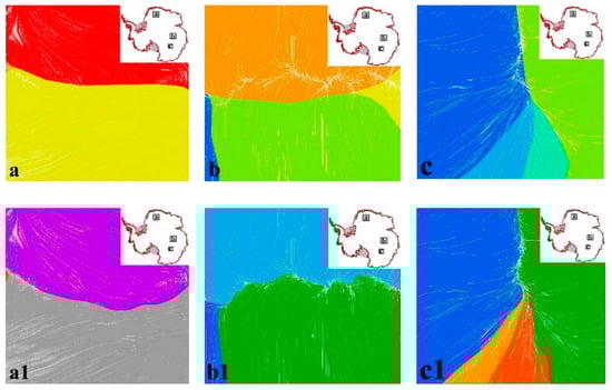
Figure 12.
Parts of detailed comparisons at the boundary of the basins between IMBIE basin systems and re-divided Antarctica basin systems. The ice flow lines belonging to different basins are rendered in different colors, where the first row (a–c) is the IMBIE basin systems and the second row (a1–c1) is the corresponding re-divided Antarctica basin systems.
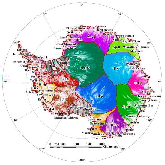
Figure 13.
Antarctic ice flow line map. The ice flow lines belonging to different basins of the re-divided Antarctic basin system are rendered in different colors.
Table 3.
Original ice basins area and boundary lengths and changes in ice basins area and boundary lengths after redefinition with ice flow lines. The max absolute values in the corresponding column are marked in BOLD fonts.
To measure the accuracy of the basin delineation results, we utilize the directional accuracy map of the proposed method, which is consistent with the resolution of the Antarctic ice flow line map. Meanwhile, directional accuracy is an essential factor for the extraction of ice flow lines. In addition, the direction of flow velocity directly determines the direction of local ice flow movement. Therefore, if the directional accuracy of the flow lines is high around the boundary lines of the redefined basins, it can be inferred that the difference between the direction of the flow lines and the direction of the flow velocity of the local ice streams in these areas is small. We take the boundary line of ice basin B-C and its fringing Amery ice shelf as the centerline to draw a buffer zone with a width of 100 km and extract the distribution of the directional accuracy obtained by the method in this paper within the range of the buffer zone. Figure 14 shows that almost all areas have an orientation accuracy of less than 1°. As listed in Table 4, more than 90% of the regions have a directional accuracy less than 1°, and more than 98% of the regions have a directional accuracy less than 3°. In addition, the mean value of these data is 0.446°, and the standard deviation is 1.181°. Thus, the ice basin delineation results are reasonable and reliable.
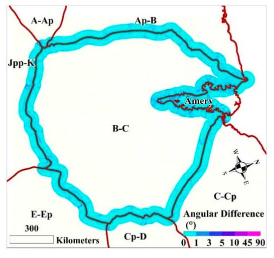
Figure 14.
Direction accuracy of B-C Basin buffer zone.
Table 4.
Cumulative frequency of the direction accuracy on B-C Basin buffer zone.
The Antarctic ice shelf system is an important area connecting the ice sheets and the ocean. Its stability is closely related to the Antarctic mass balance [49]. For the B-C basin where the major calving event occurred in July 2019 [50], the ice flow lines in the Amery ice shelf area are randomly rendered in different colors and overlaid with a Landsat 8 image collected on 14 October 2019. Based on the Antarctic IMBIE basin systems, the calving area (blue polygon in Figure 15) is delineated to the AP-B basin using the ice flow line tracing algorithm. Nevertheless, the calving area actually belongs to the B-C basin [50]. Therefore, the original basin delineation is not reasonable since the black box in Figure 15a shows the area where the ice origins are concentrated within the calving area of the Amery ice shelf. In contrast, the calving area is accurately estimated from the re-delineation of Antarctic basin systems (as shown in Figure 15b). Obviously, the re-delineation of Antarctic basin systems operates in favor of mass balance, glacier genesis and evolution.
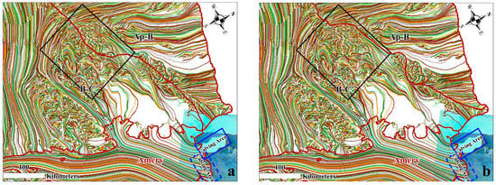
Figure 15.
Amery Ice Shelf ice flow line distribution superimposed on previous and re-divided basin results. (a) Distribution of ice flow lines superimposed on the previous basins. (b) Distribution of ice flow lines superimposed on the re-divided basins.
In summary, this paper developed a novel ice flow line extraction method by jointly considering the velocity difference, angular difference, and distance difference between ice flows. Therefore, a smooth and rational continent-scale ice flow line map is accurately generated, and the ice discharged to ice shelves from ice origins is continuously recovered to assist in the analysis of Antarctic basin system delineation, complex glacier dynamics and further mass balance. However, there are also inevitably some limitations of the proposed ice flow line extraction method. First, the basic assumption of the proposed method is that there is no ice flow crossing, which is not always true in the real world. Then, the robust estimation of ice origins is one of most important components. The introduction of multisource data as auxiliary information, such as topographic data, will be beneficial to the improvement of performance in our future work.
5. Conclusions
This paper presents a weight balance-based method using high-precision PAIVM data, where Antarctic-scale ice flow lines are extracted. To locate the pointing pixel, three impact factors, i.e., the direction difference, the distance difference, and velocity difference, are first defined to represent the directional accuracy, smoothness, and physical character. Following this, a weight balance method is used to balance the effects of these three factors by weighting. As a result, the complete trajectories of ice flow lines from their ice origins to fringing ice shelves in Antarctica are obtained, and thus the ice flow material can be effectively traced. The results show that three impact factors used to determine the pointing pixel’s position exhibit a large influence on the tracking results of the ice flow lines, which helps to extract the smooth and rational ice flow lines. Besides, our method has the best complete, smoothness compared to manual and automated methods of extracting Antarctic ice flow lines. For instance, the extracted flow lines bypass small ice features, such as islands on the surface of the ice sheet. Overlaid with the Antarctic DEM and IMBIE basin data, our results are consistent with the overall ice flow pattern with a comprehensive motion trajectory of ice discharge from their ice origins to fringing ice shelves (>90% areas). At the same time, we build on the assumption that the comprehensive ice flow lines provide more detailed information and redefine the Antarctic basin systems based on the derived ice flow lines. The redelineated Antarctic basin systems indicate a slight difference (less than 11% in area and length) from the previous IMBIE basin systems but have a higher agreement with the current ice flow patterns in Antarctic with the angular difference (over 90% of the areas) of less than 1°. Besides, the redivision of Antarctic basin systems is also of great importance to investigating the genesis and evolution of the calving event of ice shelf, such as Amery ice shelf occurred in 2019.
Author Contributions
Z.K. and Z.Y. conceived the idea. Z.Y. wrote the manuscript. Z.Y. and Z.K. discussed and revised the manuscript. All authors have read and agreed to the published version of the manuscript.
Funding
This work was supported by the National Key R&D Program of China (Grant No. 2019YFE0123300) and the National Natural Science Foundation of China (Grant Nos. 41872207).
Institutional Review Board Statement
Not applicable.
Informed Consent Statement
Not applicable.
Data Availability Statement
The Antarctic drainage basins obtained from this paper can be downloaded from the Science Data Bank (DOI:10Figure.11922/sciencedb.01562).
Acknowledgments
We truly appreciate the National Snow and Ice Data Center (https://nsidc.org/data, accessed on 7 March 2021) for providing the Antarctic ice velocity map, Antarctic Boundaries products and MODIS Mosaic of Antarctica Image Map products. We also greatly thank British Antarctic Survey (https://www.bas.ac.uk, accessed on 7 March 2021) for providing the Bedmap2 products and the US Geological Survey Earth Resources Observation Science Center for providing Landsat imagery.
Conflicts of Interest
The authors declare no conflict of interest.
References
- Dowdeswell, J.A.; Mcintyre, N. The surface topography of large ice masses from Landsat imagery. J. Glaciol. 1987, 33, 16–23. [Google Scholar] [CrossRef]
- Ely, J.C.; Clark, C.D. Flow-stripes and foliations of the Antarctic ice sheet. J. Maps 2016, 12, 249–259. [Google Scholar] [CrossRef]
- Crabtree, R.D.; Doake, C.S.M. Flow lines on Antarctic ice shelves. Polar Rec. 1980, 20, 31–37. [Google Scholar] [CrossRef]
- Fahnestock, M.; Scambos, T.; Bindschadler, R.; Kvaran, G. A millennium of variable ice flow recorded by the Ross Ice Shelf, Antarctica. J. Glaciol. 2000, 46, 652–664. [Google Scholar] [CrossRef]
- Glasser, N.; Jennings, S.J.A.; Hambrey, M.; Hubbard, B. Origin and dynamic significance of longitudinal structures (“flow stripes”) in the Antarctic Ice Sheet. Earth Surf. Dyn. 2015, 3, 239–249. [Google Scholar] [CrossRef]
- Liu, Y.; Moore, J.C.; Cheng, X.; Gladstone, R.M.; Bassis, J.N.; Liu, H.; Wen, J.; Hui, F. Ocean-driven thinning enhances iceberg calving and retreat of Antarctic ice shelves. Proc. Natl. Acad. Sci. USA 2015, 112, 3263–3268. [Google Scholar] [CrossRef]
- Glasser, N.; Scambos, T.A. A structural glaciological analysis of the 2002 Larsen B ice-shelf collapse. J. Glaciol. 2008, 54, 3–16. [Google Scholar] [CrossRef]
- Glasser, N.F.; Gudmundsson, H. Longitudinal surface structures (flowstripes) on Antarctic glaciers. Cryosphere 2012, 6, 383–391. [Google Scholar] [CrossRef]
- Das, I.; Padman, L.; Bell, R.E.; Fricker, H.A.; Tinto, K.J.; Hulbe, C.L.; Siddoway, C.S.; Dhakal, T.; Frearson, N.P.; Mosbeux, C. Multidecadal Basal Melt Rates and Structure of the Ross Ice Shelf, Antarctica, Using Airborne Ice Penetrating Radar. J. Geophys. Res. Earth Surf. 2020, 125, e2019JF005241. [Google Scholar] [CrossRef]
- Parrenin, F.; Remy, F.; Ritz, C.; Siegert, M.J.; Jouzel, J. New modeling of the Vostok ice flow line and implication for the glaciological chronology of the Vostok ice core. J. Geophys. Res. Atmos. 2004, 109, D20102. [Google Scholar] [CrossRef]
- Casassa, G.; Brecher, H. Relief and decay of flow stripes on Byrd Glacier, Antarctica. Ann. Glaciol. 1993, 17, 255–261. [Google Scholar] [CrossRef][Green Version]
- Raup, B.H.; Scambos, T.A.; Haran, T. Topography of streaklines on an Antarctic ice shelf from photoclinometry applied to a single Advanced Land Imager (ALI) image. IEEE Trans. Geosci. Remote Sens. 2005, 43, 736–742. [Google Scholar] [CrossRef]
- Young, N.; Hyland, G. Velocity and strain rates derived from InSAR analysis over the Amery Ice Shelf, East Antarctica. Ann. Glaciol. 2002, 34, 228–234. [Google Scholar] [CrossRef][Green Version]
- Shepherd, A.; Ivins, E.R.; Geruo, A.; Barletta, V.R.; Bentley, M.J.; Bettadpur, S.; Briggs, K.; Bromwich, D.H.; Forsberg, R.; Galin, N. A Reconciled Estimate of Ice-Sheet Mass Balance. Science 2012, 338, 1183–1189. [Google Scholar] [CrossRef]
- Pritchard, H.; Ligtenberg, S.R.; Fricker, H.A.; Vaughan, D.G.; van den Broeke, M.R.; Padman, L. Antarctic ice-sheet loss driven by basal melting of ice shelves. Nature 2012, 484, 502–505. [Google Scholar] [CrossRef] [PubMed]
- Rignot, E.; Velicogna, I.; van den Broeke, M.R.; Monaghan, A.; Lenaerts, J.T. Acceleration of the contribution of the Greenland and Antarctic ice sheets to sea level rise. Geophys. Res. Lett. 2011, 38, L05503. [Google Scholar] [CrossRef]
- Zhan, J.; Shi, H.; Wang, Y.; Yao, Y. Complex Principal Component Analysis of Antarctic Ice Sheet Mass Balance. Remote Sens. 2021, 13, 480. [Google Scholar] [CrossRef]
- Ferreira, V.G.; Yong, B.; Seitz, K.; Heck, B.; Grombein, T. Introducing an Improved GRACE Global Point-Mass Solution—A Case Study in Antarctica. Remote Sens. 2020, 12, 3197. [Google Scholar] [CrossRef]
- Shepherd, A.; Ivins, E.; Rignot, E.; Smith, B.; Van Den Broeke, M.; Velicogna, I.; Whitehouse, P.; Briggs, K.; Joughin, I.; Krinner, G. Mass balance of the Antarctic Ice Sheet from 1992 to 2017. Nature 2018, 558, 219–222. [Google Scholar]
- Monaghan, A.J.; Bromwich, D.H.; Fogt, R.L.; Wang, S.-H.; Mayewski, P.A.; Dixon, D.A.; Ekaykin, A.; Frezzotti, M.; Goodwin, I.; Isaksson, E. Insignificant change in Antarctic snowfall since the International Geophysical Year. Science 2006, 313, 827–831. [Google Scholar] [CrossRef]
- Rignot, E.; Bamber, J.L.; Van Den Broeke, M.R.; Davis, C.; Li, Y.; Van De Berg, W.J.; Van Meijgaard, E. Recent Antarctic ice mass loss from radar interferometry and regional climate modelling. Nat. Geosci. 2008, 1, 106–110. [Google Scholar] [CrossRef]
- Boening, C.; Lebsock, M.; Landerer, F.; Stephens, G. Snowfall-driven mass change on the East Antarctic ice sheet. Geophys. Res. Lett. 2012, 39, L21501. [Google Scholar] [CrossRef]
- Mouginot, J.; Rignot, E.; Bjørk, A.A.; Van den Broeke, M.; Millan, R.; Morlighem, M.; Noël, B.; Scheuchl, B.; Wood, M. Forty-six years of Greenland Ice Sheet mass balance from 1972 to 2018. Proc. Natl. Acad. Sci. USA 2019, 116, 9239–9244. [Google Scholar] [CrossRef] [PubMed]
- Rignot, E.; Mouginot, J.; Scheuchl, B.; Van Den Broeke, M.; Van Wessem, M.J.; Morlighem, M. Four decades of Antarctic Ice Sheet mass balance from 1979–2017. Proc. Natl. Acad. Sci. USA 2019, 116, 1095–1103. [Google Scholar] [CrossRef]
- Wingham, D.; Shepherd, A.; Muir, A.; Marshall, G. Mass balance of the Antarctic ice sheet. Philos. Trans. R. Soc. A Math. Phys. Eng. Sci. 2006, 364, 1627–1635. [Google Scholar] [CrossRef] [PubMed]
- Floricioiu, D. Drainage basin delineation for outlet glaciers of Northeast Greenland based on Sentinel-1 ice velocities and TanDEM-X elevations. Remote Sens. Environ. 2020, 237, 111483. [Google Scholar]
- Rignot, E.; Mouginot, J. Ice flow in Greenland for the international polar year 2008–2009. Geophys. Res. Lett. 2012, 39, L11501. [Google Scholar] [CrossRef]
- Weidick, A.; Williams, R.S.; Ferrigno, J.G. Satellite Image Atlas of Glaciers of the World, Greenland. In U.S. Geological Survey Professional Paper 1386-C; Williams, R.S., Ferrigno, J., Eds.; U.S. Geological Survey: Denver, CO, USA, 1995; p. 153. [Google Scholar]
- Mouginot, J.; Rignot, E.; Scheuchl, B.; Fenty, I.; Khazendar, A.; Morlighem, M.; Buzzi, A.; Paden, J. Fast retreat of Zachariæ Isstrøm, northeast Greenland. Science 2015, 350, 1357–1361. [Google Scholar] [CrossRef]
- Seleem, T.A. Analysis and Tectonic Implication of DEM-Derived Structural Lineaments, Sinai Peninsula, Egypt. Int. J. Geosci. 2013, 4, 183–201. [Google Scholar] [CrossRef]
- Glasser, N.; Jennings, S.; Hambrey, M.; Hubbard, B. Are longitudinal ice-surface structures on the Antarctic Ice Sheet indicators of long-term ice-flow configuration? Earth Surf. Dyn. Discuss. 2014, 2, 911–933. [Google Scholar]
- Budd, W.; Warner, R. A computer scheme for rapid calculations of balance-flux distributions. Ann. Glaciol. 1996, 23, 21–27. [Google Scholar] [CrossRef]
- Popov, S. Flow-lines computation and their use in subglacial geomorphology and glacial erosion modeling: The Princess Elizabeth land (East Antarctica) case study. Geomorfologiya 2017, 1, 46–54. [Google Scholar] [CrossRef]
- Glasser, N.; Scambos, T.; Bohlander, J.; Truffer, M.; Pettit, E.; Davies, B. From ice-shelf tributary to tidewater glacier: Continued rapid recession, acceleration and thinning of Röhss Glacier following the 1995 collapse of the Prince Gustav Ice Shelf, Antarctic Peninsula. J. Glaciol. 2011, 57, 397–406. [Google Scholar] [CrossRef]
- Ely, J.; Clark, C.; Ng, F.; Spagnolo, M. Insights on the formation of longitudinal surface structures on ice sheets from analysis of their spacing, spatial distribution, and relationship to ice thickness and flow. J. Geophys. Res. Earth Surf. 2017, 122, 961–972. [Google Scholar] [CrossRef]
- Tarboton, D.G. A new method for the determination of flow directions and upslope areas in grid digital elevation models. Water Resour. Res. 1997, 33, 309–319. [Google Scholar] [CrossRef]
- Casassa, G.; Jezek, K.; Turner, J.; Whillans, I. Relict flow stripes on the Ross Ice Shelf. Ann. Glaciol. 1991, 15, 132–138. [Google Scholar] [CrossRef]
- Glasser, N.; Kulessa, B.; Luckman, A.; Jansen, D.; King, E.C.; Sammonds, P.; Scambos, T.; Jezek, K. Surface structure and stability of the Larsen C ice shelf, Antarctic Peninsula. J. Glaciol. 2009, 55, 400–410. [Google Scholar] [CrossRef]
- Gudmundsson, G.H.; Raymond, C.F.; Bindschadler, R. The origin and longevity of flow stripes on Antarctic ice streams. Ann. Glaciol. 1998, 27, 145–152. [Google Scholar] [CrossRef]
- Giovinetto, M. Surface balance in ice drainage systems of Antarctica. Antarct. J. USA 1985, 20, 6–13. [Google Scholar]
- Glovinetto, M.; Zwally, H. Spatial distribution of net surface accumulation on the Antarctic ice sheet. Ann. Glaciol. 2000, 31, 171–178. [Google Scholar] [CrossRef]
- Ze, Y.; Zhizhong, K. Data from:Antarctic Drainage Basins Delineation; Science Data Bank: Beijing, China, 2022. [Google Scholar] [CrossRef]
- Mouginot, J.; Rignot, E.; Scheuchl, B. Continent-wide, interferometric SAR phase, mapping of Antarctic ice velocity. Geophys. Res. Lett. 2019, 46, 9710–9718. [Google Scholar] [CrossRef]
- Rignot, E.; Mouginot, J.; Scheuchl, B. Ice flow of the Antarctic ice sheet. Science 2011, 333, 1427–1430. [Google Scholar] [CrossRef]
- Rignot, E.; Jacobs, S.; Mouginot, J.; Scheuchl, B. Ice-shelf melting around Antarctica. Science 2013, 341, 266–270. [Google Scholar] [CrossRef]
- Mouginot, J.; Scheuchl, B.; Rignot, E. Mapping of ice motion in Antarctica using synthetic-aperture radar data. Remote Sens. 2012, 4, 2753–2767. [Google Scholar] [CrossRef]
- Fretwell, P.; Pritchard, H.D.; Vaughan, D.G.; Bamber, J.L.; Barrand, N.E.; Bell, R.; Bianchi, C.; Bingham, R.; Blankenship, D.D.; Casassa, G. Bedmap2: Improved ice bed, surface and thickness datasets for Antarctica. Cryosphere 2013, 7, 375–393. [Google Scholar] [CrossRef]
- Scambos, T.A.; Haran, T.M.; Fahnestock, M.; Painter, T.; Bohlander, J. MODIS-based Mosaic of Antarctica (MOA) data sets: Continent-wide surface morphology and snow grain size. Remote Sens. Environ. 2007, 111, 242–257. [Google Scholar] [CrossRef]
- Qi, M.; Liu, Y.; Lin, Y.; Hui, F.; Li, T.; Cheng, X. Efficient Location and Extraction of the Iceberg Calved Areas of the Antarctic Ice Shelves. Remote Sens. 2020, 12, 2658. [Google Scholar] [CrossRef]
- Francis, D.; Mattingly, K.S.; Lhermitte, S.; Temimi, M.; Heil, P. Atmospheric extremes triggered the biggest calving event in more than 50 years at the Amery Ice shelf in September 2019. Cryosphere 2021, 15, 2147–2165. [Google Scholar] [CrossRef]
Publisher’s Note: MDPI stays neutral with regard to jurisdictional claims in published maps and institutional affiliations. |
© 2022 by the authors. Licensee MDPI, Basel, Switzerland. This article is an open access article distributed under the terms and conditions of the Creative Commons Attribution (CC BY) license (https://creativecommons.org/licenses/by/4.0/).