Abstract
Rice is the staple crop for more than half the world’s population, but there is a lack of high-resolution maps outlining rice areas and their growth stages. Most remote sensing studies map the rice extent; however, in tropical regions, rice is grown throughout the year with variable planting dates and cropping frequency. Thus, mapping rice growth stages is more useful than mapping only the extent. This study addressed this challenge by developing a phenology-based method. The hypothesis was that the unsupervised classification (k-means clustering) of Sentinel-1 and 2 time-series data could identify rice fields and growth stages, because (1) the presence of flooding during transplanting can be identified by Sentinel-1 VH backscatter; and (2) changes in the canopy of rice fields during growth stages (vegetative, generative, and ripening phases) up to the point of harvesting can be identified by Normalized Difference Vegetation Index (NDVI) time series. Using the proposed method, this study mapped rice field extent and cropping calendars across Peninsular Malaysia (131,598 km2) on the Google Earth Engine (GEE) platform. The Sentinel-1 and 2 monthly time series data from January 2019 to December 2020 were classified using k-means clustering to identify areas with similar phenological patterns. This approach resulted in 10-meter resolution maps of rice field extent, intensity, and cropping calendars. Validation using very high-resolution street view images from Google Earth showed that the predicted map had an overall accuracy of 95.95%, with a kappa coefficient of 0.92. In addition, the predicted crop calendars agreed well with the local government’s granary data. The results show that the proposed phenology-based method is cost-effective and can accurately map rice fields and growth stages over large areas. The information will be helpful in measuring the achievement of self-sufficiency in rice production and estimates of methane emissions from rice cultivation.
1. Introduction
Rice is consumed by more than half of the world’s population and rice fields account for over 10% of the global cropland area. Globally, rice is the largest plant-based emitter of greenhouse gases [1]. Accurate and up-to-date information on how much rice can be produced is crucial to achieving food, climate, and water security. This is especially crucial in Malaysia, where rice is the main staple food. To ensure national food security, the government of Malaysia has set a goal of a 70% rice self-sufficiency level (SSL) [2]. Measuring the achievement of the SSL rice target requires accurate and up-to-date information on how many rice fields can be cultivated and how much of them can be harvested. Currently, information on rice fields relies on field survey data that are incomplete, time-consuming, and lack spatial details.
Remote sensing technology has been widely used to map rice fields worldwide. Moderate Resolution Imaging Spectroradiometer (MODIS) data with a high temporal resolution have been widely used for 20 years [3,4]. Although it can identify paddy fields, the coarse spatial resolution (500 m) makes it unhelpful in resolving smallholder paddy fields in Southeast Asia, which are usually less than 1 hectare [5,6,7,8]. Recently, Sentinel-1 and 2 have begun to offer high spatial (10 m) and temporal resolution (12 day) data. In addition, Sentinel-2 has two-satellite constellations, and thus its combination provides a temporal resolution of 5 days. Many studies have shown that Sentinel-1 can be used successfully for mapping rice fields in various countries, including Vietnam [9,10], China [11,12,13,14], the USA and Spain [15], India [16,17], the Mediterranean region [18], Iran [19], Bangladesh [20], South Korea [21], Indonesia and Malaysia [22], Philippines [23], Thailand [1,24], and Myanmar [25]. Concurrently, Sentinel-2 was also successfully used to map rice fields in Egypt [26] and China [27,28,29]. Several studies have used the combination of Sentinel-1 and 2 data to map rice fields, especially in temperate regions, including Japan [30], India [31], and China [32,33,34,35,36,37,38].
However, most remote sensing studies have only mapped the rice field extent. In Southeast Asia, rice is grown throughout the year, and thus, mapping the growth stages of rice fields would be more valuable. Another challenge in the tropics is that the period and frequency of cropping are variable. Each region has its own cropping calendar—for example, East Java, Indonesia, has four cropping patterns, while West Java has three patterns [39]. Thus, this study aims to fill this research gap by applying a phenological-based approach to map rice growth stages using a combination of Sentinel-1 and Sentinel-2 at a national scale. The hypothesis is that the unsupervised classification of Sentinel-1 and 2 time-series data can identify rice fields and growth stages, because (1) the presence of flooding during the transplanting can be identified by Sentinel-1 VH backscatter; and (2) changes in the canopy of rice fields during growth stages (vegetative, generative, and ripening phases) up to the point of harvesting can be identified by Normalized Difference Vegetation Index (NDVI) time series.
There are advantages and limitations for each satellite; Sentinel-1, a typical SAR, is not affected by clouds or illumination conditions. However, it has noise (speckles) that makes the map uncertain. On the other hand, Sentinel-2, an optical satellite image, is limited by cloud cover, but it provides a vegetation index directly related to rice growth stages.
Mapping rice fields using remote sensing can be broadly grouped into machine learning techniques and phenology-based approaches. The machine learning approach is based on the calibration of field observations; while accurate, it requires lots of data. The phenology-based approach relies on the knowledge of the rice growth stages, which are related to the time series of reflectance data. In particular, rice fields can be differentiated from other crops due to the presence of standing water during crop transplanting. Based on limited ground-based data, phenology-based classification can detect plant growth stages based on their vegetative cover changes (i.e., [22,40]). Most studies that use the phenology-based method are based on spectral indices and classify such indices using supervised or manual classification. There is still a lack of studies that employ unsupervised classification to differentiate spectral signatures into phenological classes.
The Google Earth Engine platform (GEE, www.earthengine.google.com, accessed on 9 April 2022) is one of the most promising developments for earth science data access and analysis [41], making the processing of multi-temporal satellite data more streamlined. The GEE provides a variety of raster data sets such as Sentinel-1 and -2, Landsat 4, 5, 7, and 8, MODIS, etc. In addition, the new datasets are periodically ingested. Furthermore, the GEE offers an interactive platform for geospatial and machine learning algorithms. Several studies have utilized the GEE platform for rice field mapping [22,29,30,34,35,40].
In a recent study, NESEA-Rice10 [40] produced a rice field extent map covering Southeast Asia (including Malaysia) and North-East Asia. The map was a new achievement because it covered a large area with high resolution (10 m). However, the map still has not been validated in tropical regions. Furthermore, NESEA-Rice10 only provides static information on where rice is grown.
Based on the research gap identified in the literature, this study introduced a phenology-based approach to map rice field extent and the cropping calendar in Peninsular Malaysia, covering over 13 million ha. This was achieved using an integration of Sentinel-1 and 2 time series data using unsupervised classification in the GEE platform. The outcomes of this study will provide an efficient framework for mapping rice fields and their growth stages, which will be valuable in tackling food security issues and mitigating methane gas emissions from rice cultivation.
2. Materials and Methods
2.1. Study Area
Peninsular Malaysia—also known as West Malaysia—covers an area of 130,598 km2, comprising 11 of 13 states of Malaysia (1°N–6.50°N and 99.50°E–104.50°E; Figure 1). The topography of the area ranges between 0 and 2187 m. The climate is classified as tropical rainforest (Af) according to the Köppen climate classification, with uniform high-humidity hot temperatures and moderate rainfall throughout the year. The average annual rainfall ranges between 1933 mm and 3080 mm [42]. The daily temperature ranges from 23–32 °C and humidity is constantly high (exceeding 68% throughout the year) [43]. Peninsular Malaysia experiences two monsoons, the northeast monsoon (NEM; November to March) and the southwest monsoon (SWM; May to September), and two short transitional periods from April to May and October to November [43,44]. Heavy rainfall events usually occur during the NEM. Maximum rainfall usually occurs during November and December, although substantial rainfall also occurs in the transitional periods (April and October). June and July during the SWM are the driest periods [44,45].
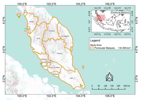
Figure 1.
Map of study area comprising of 11 states in Peninsular Malaysia.
2.2. Rice Cultivation Practices
Rice fields in Peninsular Malaysia are irrigated and have two cropping seasons. Crops during the wet season (August to February) are called the main season or are locally known as “tanaman musim utama”. Crops planted during the dry season (March to July) are called the offseason or are locally known as “tanaman luar musim” [22,46]. Due to the availability of irrigation, rice fields in Peninsular Malaysia have a diverse cropping schedule throughout the year.
Popular rice varieties planted in Peninsular Malaysia include MR 220 CL2 (97–113 days), MARDI SIRAJ 297 (105–110 days), MR 263 (97–104 days), and MR 219 (105–110 days), MRQ 74, MRQ 76, MR 220, and MR 220 CL1 [22,47,48]. MR 220 CL2 (97–113 days) is the most popular variety, planted in an around 140,146 ha area [46], with a four-month growth stage. As a generalization, the growth stages of rice are divided into four stages on a monthly basis, including T–P: tillage and planting (30 days); V: vegetative (30 days); R: reproductive (30 days); and M: maturity (30 days) [22,49].
2.3. Satelite Imagery Datasets
Sentinel-1 and 2 time-series data were retrieved from January 2019 to December 2020 from the Google Earth Engine (GEE) catalogue. Table 1 presents the characteristics of the Sentinel-1 and 2 data used in this study.

Table 1.
Characteristic of the satellite data used in this study.
Sentinel-1 ground-range-detected (S1_GRD) images with an interferometric wide swath (IW) instrument mode were used in this study. The IW mode images were provided in dual polarization with vertical transmit, vertical receive (VV) and vertical transmit, horizontal receive (VH). Only VH-polarized backscatter data were used in this study because they are more sensitive to rice fields than VV backscatter [22,50].
We only used Sentinel-1A data, as Sentinel-1B data were not available in the study area. The spatial resolution of the images was 10 m. These images were pre-processed with the Sentinel-1 Toolbox, employing thermal noise removal, radiometric calibration, and terrain correction using the SRTM 30 DEM. After pre-processing, each scene was calibrated and ortho-corrected [51].
Sentinel-2 Level-1C (Top-of-Atmosphere Reflectance, TOA) was used instead of Sentinel-2 Level-2A (Surface Reflectance, SR) because artefacts appear in Sentinel-2 Level-2A SR. In addition, Sentinel-2 Level-1C (Top-of-Atmosphere Reflectance, TOA) have been successfully used in numerous studies for surface classification, such as [28,30,32,34,52,53]. Band 4 (Red) and band 8 (NIR) from Sentinel-2 multispectral image (MSI) level 1C data were used to calculate the normalized difference vegetation index (NDVI). The spatial resolution of the images was 10 m. A total of 883 scenes from Sentinel-1A and 3,825 scenes from Sentinel-2A and B were accessed from the GEE.
2.4. Methodology
Figure 2 presents a flowchart of the methodology for this study. Each step is described in the following sections:
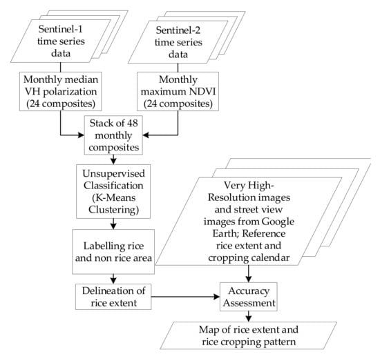
Figure 2.
Workflow of mapping rice extent and cropping calendar using fusion Sentinel-1 and 2 time-series data.
2.4.1. Generating Regions of Interest (ROI)
First, we generated the regions of interest (ROI) for each rice field location. According to the prior knowledge and information available, which were checked using very high-resolution images and street view photos from Google Earth, 31 rice fields ROIs in Peninsular Malaysia were established. The area of the ROI varied between 100 to 316,000 ha. The distribution of the ROIs can be found at the following link: https://code.earthengine.google.com/8208e211dde42d88108fbe3f5c2c420f (accessed on 9 April 2022).
2.4.2. Monthly Composite Imagery
We then compiled monthly composite data from Sentinel-1 (24 composites) and Sentinel-2 (24 Composites). Sentinel-1 SAR data were not affected by clouds; however, the data had a high noise-to-signal ratio. We used the Median Value Composite (MedVC) of the monthly time series to reduce the noise in the VH polarization data, especially in the area with overlapping data scenes [22,54].
We calculated the NDVI from the radiance on the red (band 4) and near-infrared (NIR; band 8) measured by Sentinel-2 as follows:
However, several factors can cause a considerable change to NDVI values. The most important factors are changing illumination and viewing conditions within a single image, and also between images of different days; the presence of cloud cover; and variation in atmospheric constituents—in particular, the variation in water vapour and aerosol concentrations [55]. Maximum Value Composites (MaxVCs) are generally accepted as an effective way to reduce these undesirable factors [55] and have been successfully used in studies using MODIS and SPOT data [56,57,58,59]. Thus, the MaxVCs of NDVI were used to generate the monthly composite imagery from Sentinel-2.
The monthly composite for both Sentinel-1 and 2 also addressed the issue of time alignment as the two satellites acquired images at different times. Using monthly values also allowed alignment with the rice growth stages described in Section 2.2.
2.4.3. Clustering Time Series of VH Polarization and NDVI
We used an unsupervised classification approach to group the time-series data into rice groups [60]. A total of 48 monthly composites of VH polarization and NDVI data were stacked as input into the K-Means model (i.e., the ee.Clusterer.wekaKMeans function in the GEE). The algorithm normalized the numerical inputs and used the Euclidean distance to measure distances between clusters, and iteratively modified the centroids (cluster means) to minimize within-cluster variation (distances) [22]. In total, 3000 random points for each of the ROIs were sampled as training data for training the K-Means model with 20 clusters. The GEE uses a random-point sampling approach to determine the centroids and generate the clusters. Since these points were randomly distributed across the whole region of the targeted ROI, we assumed that they adequately represented the variations of the spectra data. Moreover, the random sampling method does not require more memory computation in the GEE than the stratified random method. These random points and clusters were able to differentiate all land covers in the area (rice field, waterbody, built-up, tree).
2.4.4. Extracting Representative VH Polarization and NDVI Cluster Profiles
To extract representative VH polarization and NDVI cluster units identified by the K-means clusters, a total of 1000 samples were generated randomly for each cluster. Subsequently, spatial median values of the monthly time series for each cluster were used as the representative VH polarization and NDVI time-series profiles.
The time required by the GEE for clustering and cluster profile extraction depended on the area and the speed of internet access. For example, for a ROI of 316,000 ha, it took about 40 s to process the data using a personal computer with 16 GB RAM and a core i7 8th gen.
2.4.5. Labelling and Classification
Rice field and non-rice field areas were differentiated visually based on the representative profiles of VH and NDVI time-series data. Figure 3 shows an example of the temporal evolution of the VH polarization and NDVI cluster profile for four land-cover classes: built-up, tree, water body, and rice field. Rice fields have a unique time-series cluster profile in which the VH polarization and NDVI values fluctuate seasonally. In contrast, signals on other land covers were relatively constant, as shown in Figure 3. The median VH polarization and NDVI values for water bodies were −28.714 dB and 0.040, trees about −15.049 dB and 0.678, and built-up areas about −15.899 dB and 0.185. These values are in agreement with past studies [11,13,14,15,22,26,61]. The time that was required for interpretive cluster labelling took longer—about half an hour for each ROI—and depended on the number of rice field clusters.
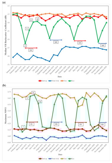
Figure 3.
Temporal evolution of the (a) VH and (b) NDVI polarization cluster profile of four land-cover classes: built-up, tree, water body and rice field; T = tillage and planting, V = vegetative, R = reproductive, M = maturity, MS = main season, OS = off season.
2.4.6. Identifying Rice Cropping Calendar
We determined the rice cropping calendar based on representative profiles of the VH and NDVI time-series data. The rice cropping calendar can be derived from rice cropping intensity and growth stages, including soil tillage and planting, as well as vegetative, reproductive, and maturity stages. For growth stages, first, the soil tillage and planting stage should be identified via VH backscatter and then followed by the next growth stages.
2.4.7. Accuracy Assessment
The accuracy of the produced maps in this study was evaluated using three types of assessment: (1) validation using virtual observations based on Google Earth VHR (very high resolution) and street view images, (2) comparison with existing rice map by NESEA-Rice10 [40], and (3) comparison with known planting and harvesting schedule.
We generated 760 random points across all ROIs across Peninsular Malaysia for the first assessment. After this, we manually evaluated each location based on VHR images from the year 2020 and Google Earth street view images, where 348 points were identified as rice fields and 392 points as non-rice. The accuracy of the rice maps was then evaluated in these virtual field data using the confusion matrix and Kappa value. Figure 4 shows an example of validating the rice area by using the Google Street View image obtained in Sungai Besar, Selangor (3°42′43.92″N, 101°03′10.93″E) in July 2019, where rice was harvested in July 2019, corresponding to Figure 3.
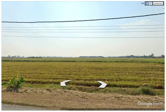
Figure 4.
Accuracy assessment by using a street view image from Google Earth in Sungai Besar, Selangor state (3°42′43.92″N, 101°03′10.93″E) in July 2019.
In the second assessment, this study’s overall accuracy and kappa coefficient were compared with those from the NESEA Rice 10 map. Finally, the third assessment compared the cropping calendar generated from this study with reference data from the granary area in Selangor state (IADA BLS) and Kedah state (MADA).
3. Results
3.1. Spectra Characteristics of Paddy Fields
Based on rice phenology, the response of the Sentinel-1 and 2 spectra to three key phenological periods (Figure 3) can be described as follows:
- The tillage and planting (T) period, where rice fields are flooded. According to the VH polarization data in Figure 3, the rice fields had a local minimum VH polarization value about <−24.5 (i.e., close to the value of a water body). This value depends on water levels or soil moisture during soil tillage. Higher water levels lead to more negative VH values [22]. On the other hand, the NDVI value during this period may not be at the required minimum due to cloud cover. Thus, Sentinel-1 data (VH polarization value) are more sensitive to detect the transplanting period than Sentinel-2 data.
- The vegetative (V) and reproductive (R) period, where rice grows rapidly with canopy closure. Consequently, increasing chlorophyll signals are accompanied by a significant decrease in soil signals [29]. NDVI values rapidly increase during this period, peaking at the end of the generative period, when the crop enters the heading or maturity stage (NDVI value was about 0.7). On the other hand, VH polarization also increases in this period and continues to rise until the end of phenology.
- The maturity (M) period. Characterized by a rapid decrease in chlorophyll content as the carotenoid content increases [29]. This distinctive drop in NDVI values indicates the maturity of the rice plant. This period occurs in the last month of the rice growth cycle.
Sentinel-1 data (VH polarization value) were more sensitive to detecting the transplanting period; on the other hand, Sentinel-2 data (NDVI value) were more detailed in showing the stages of growth and maturity. The difference between the local minimum and the peak was about four months, representing one growing season. The VH polarization and NDVI values decreased during the fallow period.
Figure 3 shows an example of a rice field cluster in Selangor that had a double cropping season in a year, where the first (October–January) and second (April–July) planting seasons were referred to as the main and off planting season, respectively. The time series profiles of VH polarization and NDVI can be designated with the four periods: T: tillage and planting (30 days); V: vegetative (30 days); R: reproductive (30 days); and M: maturity (30 days). Thus, one season of rice cropping was about 120 days or 4 months.
3.2. Accuracy of Rice Maps
Based on the unsupervised classification, rice areas throughout 31 ROIs across Peninsular Malaysia were identified. Maps of the rice extent in Peninsular Malaysia from 2019–2020 are presented in Figure 5. The complete map is available at https://rudiyanto.users.earthengine.app/view/malaysiarice, accessed on 9 April 2022. The maps produced in this study successfully distinguished rice fields from other land covers.
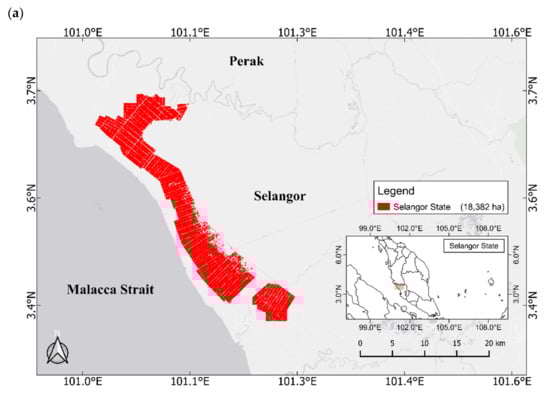
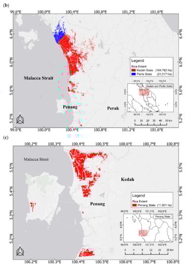
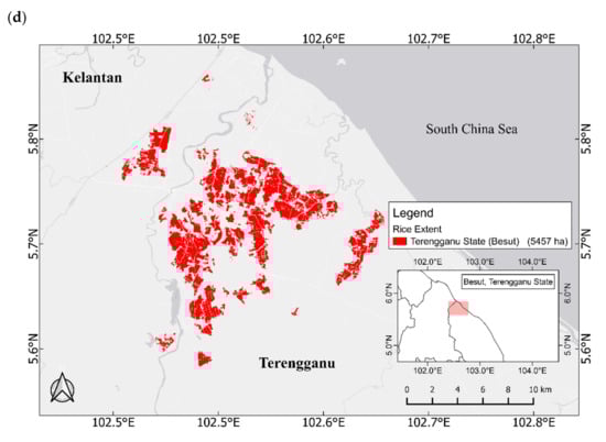
Figure 5.
Map of rice field extent in (a) Selangor State, (b) Kedah and Perlis States, (c) Penang State, and (d) Besut district, Terengganu state.
We validated our map using random sampling in the ROI of rice fields to evaluate the accuracy at a pixel level. Our map had an excellent overall accuracy of 95.95% and a kappa coefficient of 0.92, as shown in Table 2. We also evaluated the accuracy of the NESEA-Rice10 product on the same random samples. NESEA-Rice10 had a lower overall accuracy of 90.27% and a kappa coefficient of 0.80 (Table 3). Omission errors occurred when rice fields were classified as non-rice fields. Commission errors occurred when non-rice fields were classified as rice fields [22]. This study’s omission and commission errors of rice fields were 1.1% and 7.0%, respectively, while NESEA-Rice10 errors were much larger—19.9% and 1.1%, respectively. We note that outside the ROI, the NESEA-Rice10 had many speckles where non-rice areas were classified as rice.
Table 2.
Confusion matrix for the rice classification in Peninsular Malaysia by this study.
Table 3.
Confusion matrix for the rice classification in Peninsular Malaysia by NESEA-RICE 10 [40].
3.3. Cropping Calendar
A total of forty different cropping calendars of rice fields were identified across Peninsular Malaysia based on K-means spectra profiles of NDVI and VH polarization. The cropping phenological parameters of growth stages for each rice field group from January 2019 to December 2020 are listed in Table S1. Figure 6 shows the representative maps of cropping patterns with information on rice groups in each state corresponding to the cropping pattern in Table S1. For example, Selangor state had four rice groups, Kedah state had two rice groups, Perlis state had one rice group, Penang had two rice groups, and Besut district, Terengganu state had one rice group.
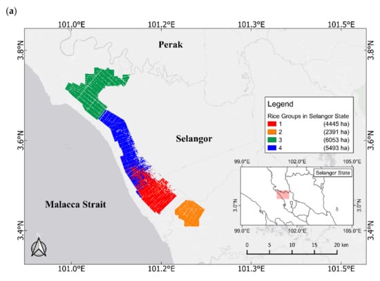
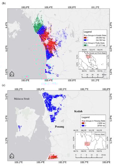
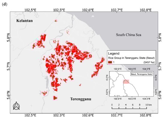
Table 4 shows an example comparison of the cropping calendar from the published granary area schedule and this study. The cropping calendar derived from this study agreed well with the granary area schedule. Peninsular Malaysia has two cropping seasons, the main season and off season, with no cash crops in-between seasons. As an example, Selangor and Kedah states had two cropping seasons in one year. In Selangor, there were four cultivated areas with different cropping schedules. The main season in 2020 in Selangor started in July, August, September, and October for Group 2, 1, 4 and 3, respectively. Concurrently, the off season started in January, February, March and April, respectively. In Kedah, two cultivated areas had different cropping schedules; the main season of both rice groups started in October, while the off season started in April and May for Groups 2 and 1 (Table 4). The Kedah and Selangor state cropping calendar correlated with the rice variety planted in the area, MR 220 CL2 (97–113 growing days).
Table 4.
Comparison of cropping calendars from granary area schedules and this study. Table 4 corresponds to Figure 6a,b. Table 4 corresponds to Table S1. T = Tillage, V = Vegetative-1, V2 = Vegetative-2, R = reproductive, M = Maturity, F (blank) = Fallow. Orange colour is the main season and green colour is the off season.
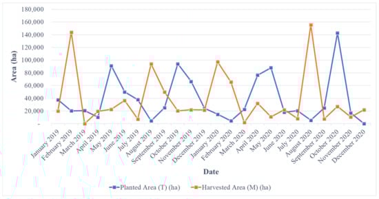
From the rice field extent and cropping calendar data in Table S1, an aggregated number of planted and harvested rice field areas in Peninsular Malaysia from 2019–2020 were generated and are shown in Figure 7. In 2019, the largest rice area was harvested in February at 143,980 ha, while in 2020 the largest area was harvested in August at 155,481 ha. There was an anomaly in April 2020 caused by the Kedah-2 cluster, which had 5 months of growth. The planting period was in April and the cluster was harvested in August over 54,782 ha. This shift was caused by rice fields that were planted at the end of April 2020 and the beginning of May 2020 and were harvested at the same time in August 2020. In 2019, Kedah-2 had 4 months of growth that started in May and finished in August. As a result, the harvested rice area in 2019 was 458,064 ha, while in 2020, it increased to 460,388 ha.
4. Discussion
4.1. Targeted ROI Processing Approach
Mapping rice fields at a fine resolution is challenging when applied to large areas such as Peninsular Malaysia. A targeted ROI processing approach was applied to reduce computational costs. This approach also allows the running of the algorithm in parallel. Rice field locations can be obtained from agricultural statistics such as those of the local government [46] or international organizations—for example, rice maps in Asia from the International Rice Research Institute (IRRI) [40]. As the rice-growing areas in Malaysia are known, the ROI can be generated for every known area. This approach significantly reduced the processing time as the classification process focused on the known rice areas to pinpoint and refine rice fields.
The targeted ROI processing approach also reduced commission errors and “salt and pepper” effects. Conventionally, non-rice areas are masked using heuristic rules to reduce the salt and pepper effect. For example, masking areas with a slope greater than 5° to remove steep terrain areas that are unsuitable for rice [40,62]; masking forest lands using Global PALSAR Forest Map 2017 [63,64]; excluding wetlands because paddy rice fields and wetlands have similar characteristics in flooding signals [65,66]; or masking sparse and natural vegetation using annual maximum vegetation index values that are less than 0.3 [35]. Although non-rice areas were reduced, other land covers may still be included in the data processing. As a result, the resulting maps still had a large amount of noise, as demonstrated by a comparison between the rice map of this study and that of NESEA-Rice10 [40] in Selangor State, Malaysia (Figure 8d). The map produced in this study shows a clearer separability between rice and non-rice areas such as roads, irrigation channels, built-up areas, and other vegetation covers (Figure 8a,b). The salt and pepper effects were significantly reduced (Figure 8c). We can see that in NESEA-Rice10, some waterbody and other vegetation covers were misclassified as rice fields (Figure 8d), which led to an overestimation of rice field extent.
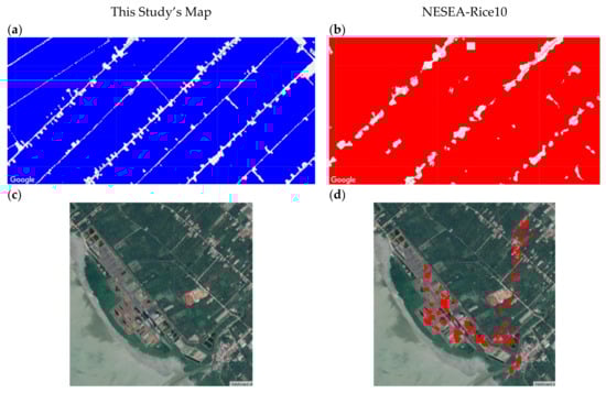
Figure 8.
Visual comparison between this study’s rice (left sides) and the NESEA-Rice10 maps (right side); (a,b) show a comparison of the separability of rice and non-rice areas; (c,d) show a comparison of salt and pepper effects. The red colour is regions classified as rice field areas; comparison location is in Selangor state, Malaysia (3°27′5.83″N, 101°7′41.18″E).
The targeted ROI processing approach also reduced the image processing time. Since K-means clustering requires many sampling points, the random sampling points in the targeted ROI approach could pick up small rice fields. This approach had an advantage in the classification of fragmented rice fields. However, accurate rice field regions need to be known beforehand in order to implement ROI-targeted processing.
4.2. Combination of Sentinel-1 and 2
This study used a combination of Sentinel-1 and 2 time series to capture the rice extent and the dynamics of rice growth. Tropical regions tend to have many clouds that interfere with optical satellite images. The Maximum Value Composite (MaxVC) of NDVI is generally used to minimize the effect of cloud cover. In rice mapping studies, the MaxVC of the NDVI has successfully minimized the effect of cloud cover in MODIS data [56,57,58,67], SPOT vegetation data [59], and Landsat-8 and Sentinel-2 data [28,34,68]. As the NDVI of water is smaller than the NDVI of clouds, cloud cover could be mistaken for water. Thus, the MaxVC of the NDVI cannot effectively detect rice fields during the transplanting period, as shown in Figure 3b. A limitation of the MaxVC of the NDVI is when there is persistent cloud cover over the study area during all revisiting times (a 5-day period) within a month. To overcome this problem, spatial interpolation [69] of NDVI values in the regions affected by clouds could be performed using machine learning models using SAR imagery and other environmental covariates [70].
On the other hand, the median of the VH polarization can detect rice fields during the transplanting period, as shown by the minimum peak in Figure 3a. However, the MaxVC of the NDVI showed better spectra discrimination than VH polarization during other growth stages. Thus, a combination of Sentinel-1 and 2 improved the overall results. The use of monthly greenest images or maximum NDVI value composites of Sentinel-2 data circumvents the need for masking clouds and cloud shadows, as is commonly carried out in rice mapping studies [64,71].
4.3. Phenology-Based and Unsupervised Classification Methods
Machine learning and deep learning approaches can be applied as classifiers when mapping rice extent and cropping calendars [10,72,73,74,75,76]. Since they are supervised classification methods, they require a large number of observations for model training. For example, a recent study [52] used 21,696 observations to train a convolutional neural network (CNN) model to map rice extent and growth stages in West Java, Indonesia. On the other hand, the phenology-based method used in this study does not require many observations. Our method based on k-means clustering can quickly identify rice fields from expert interpretation due to the unique spectra pattern of VH polarization and the NDVI of rice fields from Sentinel-1 and 2, respectively, resulting in high—up to 96%—accuracy rice maps. Due to its ability to generalize clusters from the data pattern, the k-means method can learn from the data and group time series into unique spectral responses related to rice phenology or other land uses. The method was also able to identify reflectance signatures due to soil tillage and planting, vegetative, reproductive, and ripening stages, as shown in Section 3.1. Nevertheless, to identify the reflectance signature, prior knowledge is required. To overcome this limitation, K-means and supervised methods such as random forest [75] can be combined to automatically produce rice extent and growth stage maps.
An important feature of this study was the ability to map cropping intensity and cropping calendar data. RiceAtlas [77] and RICA [78] provide rice calendar and production data from around the world and rice crop calendars for Asia, respectively. However, those studies only present information on cropping calendars at the country level. In reality, the cropping calendar varies significantly within countries and could change due to local conditions. Using a phenology-based method, we have provided not only maps of rice extent but also cropping intensity and calendar at the pixel level. We have demonstrated that the unsupervised classification of Sentinel-1 and 2 time-series data and their implementation in the GEE is cost-effective in mapping rice extent, intensity, and calendars. In addition, the approach is scalable, and GEE can process data of vast areas [40,79].
4.4. Mapping Rice Extent in Tropical Regions
Our methods were applied in rice fields in tropical regions that are planted throughout the year with different planting dates and frequencies. In South-East Asia, different places can have different rice cropping calendars due to variable irrigation schemes. The novelty of our method is that it can handle the complexity of rice fields in tropical regions. Most previous studies have used Sentinel-1 and 2 for mapping rice in temperate regions such as Japan [30], China [32,33,34,35,36,37,38], and India [31], which are only planted in summer. Our methods can map rice fields rapidly—in less than an hour for 100,000 ha—as rice fields can be easily identified from their unique phenology spectra without extensive surveys. Thus, our method has a high potential and capability for application in other regions.
4.5. Sources of Uncertainty
Although the present results clearly show the high accuracy of the rice-mapping procedure, it is appropriate to recognize several potential limitations. Errors usually occurred at the perimeter between rice and non-rice fields (Figure 9), leading to omission errors in the rice field category. The mixed pixel effect in the boundaries along the field edge contributed to the discrepancy. This effect has been reported in rice mapping studies and is still a source of spatial uncertainty [3,15,20,22,50,73]. For the commission errors in the rice field category, the contribution was mainly from non-rice fields (such as small roads, levees, or bunds) classified as rice fields. Bunds are similar to rice fields, as their water levels and soil moisture also fluctuate seasonally.
Figure 9.
Sources of error in rice field classification. The green colour shows regions classified as rice field areas, while the rest were non-rice areas in Kedah State (6°6′41.10″N, 100°22′58.91″E).
5. Conclusions
Our results support the hypothesis that the integration of Sentinel-1 and 2 time-series data using a phenology-based method in the GEE cloud computing platform can accurately produce maps of rice extent, cropping intensity, and cropping calendars. Furthermore, the proposed method produced rice extent and growth-stage maps with a high spatial resolution (10 m) over a large region.
The results show that the proposed method had a high overall map accuracy of 95.95%, with a kappa coefficient of 0.92. The method distinguished rice growing stages and established that most of the rice fields in Peninsular Malaysia had two cropping seasons a year.
The proposed methodology had several advantages compared to past studies:
- It produces not only high-resolution maps of rice extent but also of intensity and cropping calendars in tropical regions due to the use of both Sentinel-1 and 2 time series data;
- It produces high-accuracy maps rapidly without extensive field survey data due to the use of an unsupervised K-Means method in the GEE;
- It reduces salt and pepper effects due to the use of targeted regions of interest;
- It eliminates the need for masking clouds and cloud shadows due to the use of monthly greenest images or maximum NDVI value composites of Sentinel-2 data;
- It is able to identify the signatures of rice phenology stages, including soil tillage and planting, vegetative, reproductive, and ripening stages due to the fusion of Sentinel-1 and 2 time series data.
The results presented in this paper could be used as a complementary source of information to field survey data. This information is necessary to achieve the United Nations 2030 Agenda for the Sustainable Development Goals (SDGs) [80]—particularly Goal 2, Zero Hunger. As paddy rice consumes a large amount of water, this data can be used to address water security management (SDG Goal 6). Rice fields are also an important source of methane, and the spatial information can be used for greenhouse gas accounting (SDG Goal 6). Finally, the data can help form government policies to address national food security to reduce poverty (Goal 1).
Supplementary Materials
The following supporting information can be downloaded at: https://www.mdpi.com/article/10.3390/rs14081875/s1, Table S1: Growth stages from generalized phenological parameters for rice clusters in rice fields in the Peninsular Malaysia, Malaysia. Table S1 corresponds to Figure 5, Figure 6 and Figure 7 and Table 4. T = Tillage, V = Vegetative-1, V2 = Vegetative-2, R = reproductive, M = Maturity, F (blank) = Fallow. The code built for the mapping is available at https://code.earthengine.google.com/6120f79168e4f520a56b9d43eff10d60, (accessed on 10 April 2022). Comparison between the rice extent map product from this study and NESEA-Rice10 is available at https://rudiyanto.users.earthengine.app/view/malaysiarice, (accessed on 10 April 2022).
Author Contributions
Conceptualization, R., B.I.S., B.M., R.M.S., N.C.S. and S.G.E.G.; methodology, R. and B.M.; software, F. and R.; validation, F. and R.; formal analysis, F. and R.; investigation, F. and R.; resources, F. and R.; data curation, F. and R.; writing—original draft preparation, F. and R.; writing—review and editing, B.M.; visualization, F. All authors have read and agreed to the published version of the manuscript.
Funding
This work was supported by Talent & Publication Enhancement-Research Grant (TAPE-RG) Dana Penyelidikan Universiti Malaysia Terengganu (DP–UMT), Vot. No. 55246, UMT/CRIM/2-2/2/14 Jld.4 (68). The computational aspect of this study was supported by The Group on Earth Observations (GEO) and Google Earth Engine (GEE) award.
Conflicts of Interest
The authors declare no conflict of interest.
References
- Xu, L.; Zhang, H.; Wang, C.; Wei, S.; Zhang, B.; Wu, F.; Tang, Y. Paddy rice mapping in thailand using time-series sentinel-1 data and deep learning model. Remote Sens. 2021, 13, 3994. [Google Scholar] [CrossRef]
- Ministry of Agriculture and Food Industries. Dasar Agromakanan Negara 2011–2020; Ministry of Agriculture and Food Industries: Putrajaya, Malaysia, 2011; ISBN 9789839863390.
- Xiao, X.; Boles, S.; Frolking, S.; Li, C.; Babu, J.Y.; Salas, W.; Moore, B. Mapping paddy rice agriculture in South and Southeast Asia using multi-temporal MODIS images. Remote Sens. Environ. 2006, 100, 95–113. [Google Scholar] [CrossRef]
- Xiao, X.; Boles, S.; Liu, J.; Zhuang, D.; Frolking, S.; Li, C.; Salas, W.; Moore, B. Mapping paddy rice agriculture in southern China using multi-temporal MODIS images. Remote Sens. Environ. 2005, 95, 480–492. [Google Scholar] [CrossRef]
- Shew, A.M.; Ghosh, A. Identifying dry-season rice-planting patterns in bangladesh using the landsat archive. Remote Sens. 2019, 11, 1235. [Google Scholar] [CrossRef]
- Dong, J.; Xiao, X.; Zhang, G.; Menarguez, M.A.; Choi, C.Y.; Qin, Y.; Luo, P.; Zhang, Y.; Moore, B. Northward expansion of paddy rice in northeastern Asia during 2000–2014. Geophys. Res. Lett. 2016, 43, 3754–3761. [Google Scholar] [CrossRef]
- Liu, Z.; Hu, Q.; Tan, J.; Zou, J. Regional scale mapping of fractional rice cropping change using a phenology-based temporal mixture analysis. Int. J. Remote Sens. 2019, 40, 2703–2716. [Google Scholar] [CrossRef]
- Dong, J.; Xiao, X.; Kou, W.; Qin, Y.; Zhang, G.; Li, L.; Jin, C.; Zhou, Y.; Wang, J.; Biradar, C.; et al. Tracking the dynamics of paddy rice planting area in 1986–2010 through time series Landsat images and phenology-based algorithms. Remote Sens. Environ. 2015, 160, 99–113. [Google Scholar] [CrossRef]
- Lasko, K.; Vadrevu, K.P.; Tran, V.T.; Justice, C. Mapping Double and Single Crop Paddy Rice with Sentinel-1A at Varying Spatial Scales and Polarizations in Hanoi, Vietnam. IEEE J. Sel. Top. Appl. Earth Obs. Remote Sens. 2018, 11, 498–512. [Google Scholar] [CrossRef]
- Son, N.T.; Chen, C.F.; Chen, C.R.; Minh, V.Q. Assessment of Sentinel-1A data for rice crop classification using random forests and support vector machines. Geocarto Int. 2018, 33, 587–601. [Google Scholar] [CrossRef]
- Yang, H.; Pan, B.; Wu, W.; Tai, J. Field-based rice classification in Wuhua county through integration of multi-temporal Sentinel-1A and Landsat-8 OLI data. Int. J. Appl. Earth Obs. Geoinf. 2018, 69, 226–236. [Google Scholar] [CrossRef]
- Tian, H.; Wu, M.; Wang, L.; Niu, Z. Mapping early, middle and late rice extent using Sentinel-1A and Landsat-8 data in the poyang lake plain, China. Sensors 2018, 18, 185. [Google Scholar] [CrossRef] [PubMed]
- Mansaray, L.R.; Zhang, D.; Zhou, Z.; Huang, J. Evaluating the potential of temporal Sentinel-1A data for paddy rice discrimination at local scales. Remote Sens. Lett. 2017, 8, 967–976. [Google Scholar] [CrossRef]
- Mansaray, L.R.; Huang, W.; Zhang, D.; Huang, J.; Li, J. Mapping rice fields in urban Shanghai, southeast China, using Sentinel-1A and Landsat 8 datasets. Remote Sens. 2017, 9, 257. [Google Scholar] [CrossRef]
- Clauss, K.; Ottinger, M.; Kuenzer, C. Mapping rice areas with Sentinel-1 time series and superpixel segmentation. Int. J. Remote Sens. 2018, 39, 1399–1420. [Google Scholar] [CrossRef]
- Mohite, J.D.; Sawant, S.A.; Kumar, A.; Prajapati, M.; Pusapati, S.V.; Singh, D.; Pappula, S. Operational near real time rice area mapping using multi-temporal sentinel-1 sar observations. Int. Arch. Photogramm. Remote Sens. Spat. Inf. Sci. 2018, 42, 507–514. [Google Scholar] [CrossRef]
- Mandal, D.; Kumar, V.; Bhattacharya, A.; Rao, Y.S.; Siqueira, P.; Bera, S. Sen4Rice: A processing chain for differentiating early and late transplanted rice using time-series sentinel-1 SAR data with google earth engine. IEEE Geosci. Remote Sens. Lett. 2018, 15, 1947–1951. [Google Scholar] [CrossRef]
- Nguyen, D.B.; Wagner, W. European rice cropland mapping with Sentinel-1 data: The mediterranean region case study. Water 2017, 9, 392. [Google Scholar] [CrossRef]
- Saadat, M.; Hasanlou, M.; Homayouni, S. Rice crop mapping using sentinel-1 time series images (case study: Mazandaran, Iran). Int. Arch. Photogramm. Remote Sens. Spat. Inf. Sci. 2019, 42, 897–904. [Google Scholar] [CrossRef]
- Singha, M.; Dong, J.; Zhang, G.; Xiao, X. High resolution paddy rice maps in cloud-prone Bangladesh and Northeast India using Sentinel-1 data. Sci. Data 2019, 6, 26. [Google Scholar] [CrossRef]
- Park, S.; Im, J.; Park, S.; Yoo, C.; Han, H.; Rhee, J. Classification and mapping of paddy rice by combining Landsat and SAR time series data. Remote Sens. 2018, 10, 447. [Google Scholar] [CrossRef]
- Rudiyanto; Minasny, B.; Shah, R.M.; Soh, N.C.; Arif, C.; Setiawan, B.I. Automated Near-Real-Time Mapping and Monitoring of Rice Extent, Cropping Patterns, and Growth Stages in Southeast Asia Using Sentinel-1 Time Series on a Google Earth Engine Platform. Remote Sens. 2019, 11, 1666. [Google Scholar] [CrossRef]
- Fikriyah, V.N.; Darvishzadeh, R.; Laborte, A.; Khan, N.I.; Nelson, A. Discriminating transplanted and direct seeded rice using Sentinel-1 intensity data. Int. J. Appl. Earth Obs. Geoinf. 2019, 76, 143–153. [Google Scholar] [CrossRef]
- Setiyono, T.D.; Quicho, E.D.; Holecz, F.H.; Khan, N.I.; Romuga, G.; Maunahan, A.; Garcia, C.; Rala, A.; Raviz, J.; Collivignarelli, F.; et al. Rice yield estimation using synthetic aperture radar (SAR) and the ORYZA crop growth model: Development and application of the system in South and South-east Asian countries. Int. J. Remote Sens. 2018, 40, 8093–8124. [Google Scholar] [CrossRef]
- Torbick, N.; Chowdhury, D.; Salas, W.; Qi, J. Monitoring Rice Agriculture across Myanmar Using Time Series Sentinel-1 Assisted by Landsat-8 and PALSAR-2. Remote Sens. 2017, 9, 119. [Google Scholar] [CrossRef]
- Ali, A.M.; Savin, I.; Poddubskiy, A.; Abouelghar, M.; Saleh, N.; Abutaleb, K.; El-Shirbeny, M.; Dokukin, P. Integrated method for rice cultivation monitoring using Sentinel-2 data and Leaf Area Index. Egypt J. Remote Sens. Sp. Sci. 2020, 24, 431–441. [Google Scholar] [CrossRef]
- You, N.; Dong, J.; Huang, J.; Du, G.; Zhang, G.; He, Y.; Yang, T.; Di, Y.; Xiao, X. The 10-m crop type maps in Northeast China during 2017–2019. Sci. Data 2021, 8, 41. [Google Scholar] [CrossRef]
- Liu, L.; Xiao, X.; Qin, Y.; Wang, J.; Xu, X.; Hu, Y.; Qiao, Z. Mapping cropping intensity in China using time series Landsat and Sentinel-2 images and Google Earth Engine. Remote Sens. Environ. 2020, 239, 111624. [Google Scholar] [CrossRef]
- Ni, R.; Tian, J.; Li, X.; Yin, D.; Li, J.; Gong, H.; Zhang, J.; Zhu, L.; Wu, D. An enhanced pixel-based phenological feature for accurate paddy rice mapping with Sentinel-2 imagery in Google Earth Engine. ISPRS J. Photogramm. Remote Sens. 2021, 178, 282–296. [Google Scholar] [CrossRef]
- Inoue, S.; Ito, A.; Yonezawa, C. Mapping Paddy fields in Japan by using a Sentinel-1 SAR time series supplemented by Sentinel-2 images on Google Earth Engine. Remote Sens. 2020, 12, 1622. [Google Scholar] [CrossRef]
- Ferrant, S.; Selles, A.; Le Page, M.; Herrault, P.A.; Pelletier, C.; Al-Bitar, A.; Mermoz, S.; Gascoin, S.; Bouvet, A.; Saqalli, M.; et al. Detection of irrigated crops from Sentinel-1 and Sentinel-2 data to estimate seasonal groundwater use in South India. Remote Sens. 2017, 9, 1119. [Google Scholar] [CrossRef]
- Zhang, X.; Wu, B.; Ponce-Campos, G.E.; Zhang, M.; Chang, S.; Tian, F. Mapping up-to-date paddy rice extent at 10 M resolution in China through the integration of optical and synthetic aperture radar images. Remote Sens. 2018, 10, 1200. [Google Scholar] [CrossRef]
- Cai, Y.; Lin, H.; Zhang, M. Mapping paddy rice by the object-based random forest method using time series Sentinel-1/Sentinel-2 data. Adv. Space Res. 2019, 64, 2233–2244. [Google Scholar] [CrossRef]
- Luo, C.; Liu, H.-J.; Lu, L.-P.; Liu, Z.-R.; Kong, F.-C.; Zhang, X.-L. Monthly composites from Sentinel-1 and Sentinel-2 images for regional major crop mapping with Google Earth Engine. J. Integr. Agric. 2021, 20, 1944–1957. [Google Scholar] [CrossRef]
- Xiao, W.; Xu, S.; He, T. Object-Based Algorithm—A Implementation in Hangjiahu Plain in China Using GEE Platform. Remote Sens. 2021, 13, 990. [Google Scholar] [CrossRef]
- You, N.; Dong, J. Examining earliest identifiable timing of crops using all available Sentinel 1/2 imagery and Google Earth Engine. ISPRS J. Photogramm. Remote Sens. 2020, 161, 109–123. [Google Scholar] [CrossRef]
- Wu, W.; Wang, W.; Meadows, M.E.; Yao, X.; Peng, W. Cloud-based typhoon-derived paddy rice flooding and lodging detection using multi-temporal Sentinel-1&2. Front. Earth Sci. 2019, 13, 682–694. [Google Scholar] [CrossRef]
- He, Y.; Dong, J.; Liao, X.; Sun, L.; Wang, Z.; You, N.; Li, Z.; Fu, P. Examining rice distribution and cropping intensity in a mixed single- and double-cropping region in South China using all available Sentinel 1/2 images. Int. J. Appl. Earth Obs. Geoinf. 2021, 101, 102351. [Google Scholar] [CrossRef]
- Ramadhani, F.; Pullanagari, R.; Kereszturi, G.; Procter, J. Automatic mapping of rice growth stages using the integration of sentinel-2, mod13q1, and sentinel-1. Remote Sens. 2020, 12, 3613. [Google Scholar] [CrossRef]
- Han, J.; Zhang, Z.; Luo, Y.; Cao, J.; Zhang, L.; Cheng, F.; Zhuang, H.; Zhang, J. AsiaRiceMap10m: High-resolution annual paddy rice maps for Southeast and Northeast Asia from 2017 to 2019. Earth Syst. Sci. Data Discuss. 2021, 211, 1–27. [Google Scholar] [CrossRef]
- Gorelick, N.; Hancher, M.; Dixon, M.; Ilyushchenko, S.; Thau, D.; Moore, R. Remote Sensing of Environment Google Earth Engine: Planetary-scale geospatial analysis for everyone. Remote Sens. Environ. 2017, 202, 18–27. [Google Scholar] [CrossRef]
- Nashwan, M.S.; Shahid, S.; Chung, E.S.; Ahmed, K.; Song, Y.H. Development of climate-based index for hydrologic hazard susceptibility. Sustainability 2018, 10, 2182. [Google Scholar] [CrossRef]
- Khan, N.; Pour, S.H.; Shahid, S.; Ismail, T.; Ahmed, K.; Chung, E.S.; Nawaz, N.; Wang, X. Spatial distribution of secular trends in rainfall indices of Peninsular Malaysia in the presence of long-term persistence. Meteorol. Appl. 2019, 26, 655–670. [Google Scholar] [CrossRef]
- Pour, S.H.; Bin Harun, S.; Shahid, S. Genetic Programming for the Downscaling of Extreme Rainfall Events on the East Coast of Peninsular Malaysia. Atmosphere 2014, 5, 914–936. [Google Scholar] [CrossRef]
- Mayowa, O.O.; Pour, S.H.; Shahid, S.; Mohsenipour, M.; Bin Harun, S.; Heryansyah, A.; Ismail, T. Trends in rainfall and rainfall-related extremes in the east coast of peninsular Malaysia. J. Earth Syst. Sci. 2015, 124, 1609–1622. [Google Scholar] [CrossRef]
- Department of Agriculture Peninsular Malaysia. Paddy Statistics of Malaysia 2015; Department of Agriculture Peninsular Malaysia: Putrajaya, Malaysia, 2016.
- Nazuri, N.S.; Man, N. Acceptance and Practices on New Paddy Seed Variety Among Farmers in MADA Granary Area. Acad. J. Interdiscip. Stud. 2016, 5, 105–110. [Google Scholar] [CrossRef][Green Version]
- Sarena, C.O.; Ashraf, S.; Siti Aiysyah, T. The Status of the Paddy and Rice Industry in Malaysia; Khazanah Research Institute: Kuala Lumpur, Malaysia, 2019; ISBN 9789671633571. [Google Scholar]
- Sianturi, R.; Jetten, V.G.; Sartohadi, J. Mapping cropping patterns in irrigated rice fields in West Java: Towards mapping vulnerability to flooding using time-series MODIS imageries. Int. J. Appl. Earth Obs. Geoinf. 2018, 66, 1–13. [Google Scholar] [CrossRef]
- Nguyen, D.B.; Gruber, A.; Wagner, W. Mapping rice extent and cropping scheme in the Mekong Delta using Sentinel-1A data. Remote Sens. Lett. 2016, 7, 1209–1218. [Google Scholar] [CrossRef]
- Google Developers Sentinel-1 Algorithm. Available online: https://developers.google.com/earth-engine/guides/sentinel1 (accessed on 10 March 2022).
- Thorp, K.R.; Drajat, D. Deep machine learning with Sentinel satellite data to map paddy rice production stages across West Java, Indonesia. Remote Sens. Environ. 2021, 265, 112679. [Google Scholar] [CrossRef]
- Slagter, B.; Tsendbazar, N.E.; Vollrath, A.; Reiche, J. Mapping wetland characteristics using temporally dense Sentinel-1 and Sentinel-2 data: A case study in the St. Lucia wetlands, South Africa. Int. J. Appl. Earth Obs. Geoinf. 2020, 86, 102009. [Google Scholar] [CrossRef]
- Clauss, K.; Ottinger, M.; Leinenkugel, P.; Kuenzer, C. Estimating rice production in the Mekong Delta, Vietnam, utilizing time series of Sentinel-1 SAR data. Int. J. Appl. Earth Obs. Geoinf. 2018, 73, 574–585. [Google Scholar] [CrossRef]
- Holben, B.N. Characteristics of maximum-value composite images from temporal AVHRR data. Int. J. Remote Sens. 1986, 7, 1417–1434. [Google Scholar] [CrossRef]
- De Bie, C.A.J.M.; Nguyen, T.T.H.; Ali, A.; Scarrott, R.; Skidmore, A.K. LaHMa: A landscape heterogeneity mapping method using hyper-temporal datasets. Int. J. Geogr. Inf. Sci. 2012, 26, 2177–2192. [Google Scholar] [CrossRef]
- Gumma, M.K.; Thenkabail, P.S.; Maunahan, A.; Islam, S.; Nelson, A. Mapping seasonal rice cropland extent and area in the high cropping intensity environment of Bangladesh using MODIS 500m data for the year 2010. ISPRS J. Photogramm. Remote Sens. 2014, 91, 98–113. [Google Scholar] [CrossRef]
- Gumma, M.K. Mapping rice areas of South Asia using MODIS multitemporal data. J. Appl. Remote Sens. 2011, 5, 053547. [Google Scholar] [CrossRef]
- Nguyen, T.T.H.; De Bie, C.A.J.M.; Ali, A.; Smaling, E.M.A.; Chu, T.H. Mapping the irrigated rice cropping patterns of the Mekong delta, Vietnam, through hyper-temporal spot NDVI image analysis. Int. J. Remote Sens. 2012, 33, 415–434. [Google Scholar] [CrossRef]
- Aguilar, A. Machine Learning and Big Data Techniques for Satellite-Based Rice Phenology Monitoring. Ph.D. Thesis, University of Manchester, Manchester, UK, 2019. [Google Scholar]
- Zhang, X.; Yang, G.; Xu, X.; Yao, X.; Zheng, H.; Zhu, Y.; Cao, W.; Cheng, T. An assessment of Planet satellite imagery for county-wide mapping of rice planting areas in Jiangsu Province, China with one-class classification approaches. Int. J. Remote Sens. 2021, 42, 7610–7635. [Google Scholar] [CrossRef]
- Sun, H.S.; Huang, J.F.; Huete, A.R.; Peng, D.L.; Zhang, F. Mapping paddy rice with multi-date moderate-resolution imaging spectroradiometer (MODIS) data in China. J. Zhejiang Univ. Sci. A 2009, 10, 1509–1522. [Google Scholar] [CrossRef]
- Zhang, G.; Xiao, X.; Biradar, C.M.; Dong, J.; Qin, Y.; Menarguez, M.A.; Zhou, Y.; Zhang, Y.; Jin, C.; Wang, J.; et al. Spatiotemporal patterns of paddy rice croplands in China and India from 2000 to 2015. Sci. Total Environ. 2017, 579, 82–92. [Google Scholar] [CrossRef]
- Wang, J.; Xiao, X.; Qin, Y.; Dong, J.; Zhang, G.; Kou, W.; Jin, C.; Zhou, Y.; Zhang, Y. Mapping paddy rice planting area in wheat-rice double-cropped areas through integration of Landsat-8 OLI, MODIS, and PALSAR images. Sci. Rep. 2015, 5, 10088. [Google Scholar] [CrossRef]
- Zhang, G.; Xiao, X.; Dong, J.; Kou, W.; Jin, C.; Qin, Y.; Zhou, Y.; Wang, J.; Menarguez, M.A.; Biradar, C. Mapping paddy rice planting areas through time series analysis of MODIS land surface temperature and vegetation index data. ISPRS J. Photogramm. Remote Sens. 2015, 106, 157–171. [Google Scholar] [CrossRef]
- Zhou, Y.; Xiao, X.; Qin, Y.; Dong, J.; Zhang, G.; Kou, W.; Jin, C.; Wang, J.; Li, X. Mapping paddy rice planting area in rice-wetland coexistent areas through analysis of Landsat 8 OLI and MODIS images. Int. J. Appl. Earth Obs. Geoinf. 2016, 46, 1–12. [Google Scholar] [CrossRef] [PubMed]
- Yeom, J.M.; Kim, H.O. Comparison of NDVIs from GOCI and MODIS data towards improved assessment of crop temporal dynamics in the case of paddy rice. Remote Sens. 2015, 7, 11326–11343. [Google Scholar] [CrossRef]
- Pan, L.; Xia, H.; Yang, J.; Niu, W.; Wang, R.; Song, H.; Guo, Y.; Qin, Y. Mapping cropping intensity in Huaihe basin using phenology algorithm, all Sentinel-2 and Landsat images in Google Earth Engine. Int. J. Appl. Earth Obs. Geoinf. 2021, 102, 102376. [Google Scholar] [CrossRef]
- Guo, Y.; Xia, H.; Pan, L.; Zhao, X.; Li, R. Mapping the Northern Limit of Double Cropping Using a Phenology-Based Algorithm and Google Earth Engine. Remote Sens. 2022, 14, 1004. [Google Scholar] [CrossRef]
- Dos Santos, E.P.; Da Silva, D.D.; Do Amaral, C.H.; Fernandes-Filho, E.I.; Dias, R.L.S. A Machine Learning approach to reconstruct cloudy affected vegetation indices imagery via data fusion from Sentinel-1 and Landsat 8. Comput. Electron. Agric. 2022, 194, 106753. [Google Scholar] [CrossRef]
- Qin, Y.; Xiao, X.; Dong, J.; Zhou, Y.; Zhu, Z.; Zhang, G.; Du, G.; Jin, C.; Kou, W.; Wang, J.; et al. Mapping paddy rice planting area in cold temperate climate region through analysis of time series Landsat 8 (OLI), Landsat 7 (ETM+) and MODIS imagery. ISPRS J. Photogramm. Remote Sens. 2015, 105, 220–233. [Google Scholar] [CrossRef]
- Zhang, M.; Lin, H.; Wang, G.; Sun, H.; Fu, J. Mapping paddy rice using a Convolutional Neural Network (CNN) with Landsat 8 datasets in the Dongting Lake Area, China. Remote Sens. 2018, 10, 1840. [Google Scholar] [CrossRef]
- Clauss, K.; Yan, H.; Kuenzer, C. Mapping paddy rice in China in 2002, 2005, 2010 and 2014 with MODIS time series. Remote Sens. 2016, 8, 434. [Google Scholar] [CrossRef]
- De Bem, P.P.; de Carvalho Júnior, O.A.; de Carvalho, O.L.F.; Gomes, R.A.T.; Guimarāes, R.F.; Pimentel, C.M.M. Irrigated rice crop identification in Southern Brazil using convolutional neural networks and Sentinel-1 time series. Remote Sens. Appl. Soc. Environ. 2021, 24, 100627. [Google Scholar] [CrossRef]
- Padarian, J.; Minasny, B.; McBratney, A.B. Machine learning and soil sciences: A review aided by machine learning tools. Soil 2020, 6, 35–52. [Google Scholar] [CrossRef]
- Padarian, J.; Minasny, B.; McBratney, A.B. Using deep learning for digital soil mapping. Soil 2019, 5, 79–89. [Google Scholar] [CrossRef]
- Laborte, A.G.; Gutierrez, M.A.; Balanza, J.G.; Saito, K.; Zwart, S.J.; Boschetti, M.; Murty, M.V.R.; Villano, L.; Aunario, J.K.; Reinke, R.; et al. RiceAtlas, a spatial database of global rice calendars and production. Sci. Data 2017, 4, 170074. [Google Scholar] [CrossRef] [PubMed]
- Mishra, B.; Busetto, L.; Boschetti, M.; Laborte, A.; Nelson, A. RICA: A rice crop calendar for Asia based on MODIS multi year data. Int. J. Appl. Earth Obs. Geoinf. 2021, 103, 102471. [Google Scholar] [CrossRef]
- Dong, J.; Xiao, X.; Menarguez, M.A.; Zhang, G.; Qin, Y.; Thau, D.; Biradar, C.; Moore, B. Mapping paddy rice planting area in northeastern Asia with Landsat 8 images, phenology-based algorithm and Google Earth Engine. Remote Sens. Environ. 2016, 185, 142–154. [Google Scholar] [CrossRef]
- United Nations General Assembly About the Sustainable Development Goals-United Nations Sustainable Development. Available online: https://sdgs.un.org/goals (accessed on 4 September 2021).
Publisher’s Note: MDPI stays neutral with regard to jurisdictional claims in published maps and institutional affiliations. |
© 2022 by the authors. Licensee MDPI, Basel, Switzerland. This article is an open access article distributed under the terms and conditions of the Creative Commons Attribution (CC BY) license (https://creativecommons.org/licenses/by/4.0/).