Automatic Semantic Segmentation of Benthic Habitats Using Images from Towed Underwater Camera in a Complex Shallow Water Environment

Abstract

Underwater image segmentation is useful for benthic habitat mapping and monitoring; however, manual annotation is time-consuming and tedious. We propose automated segmentation of benthic habitats using unsupervised semantic algorithms. Four such algorithms––Fast and Robust Fuzzy C-Means (FR), Superpixel-Based Fast Fuzzy C-Means (FF), Otsu clustering (OS), and K-means segmentation (KM)––were tested for accuracy for segmentation. Further, YCbCr and the Commission Internationale de l’Éclairage (CIE) LAB color spaces were evaluated to correct variations in image illumination and shadow effects. Benthic habitat field data from a geo-located high-resolution towed camera were used to evaluate proposed algorithms. The Shiraho study area, located off Ishigaki Island, Japan, was used, and six benthic habitats were classified. These categories were corals (Acropora and Porites), blue corals (Heliopora coerulea), brown algae, other algae, sediments, and seagrass (Thalassia hemprichii). Analysis showed that the K-means clustering algorithm yielded the highest overall accuracy. However, the differences between the KM and OS overall accuracies were statistically insignificant at the 5% level. Findings showed the importance of eliminating underwater illumination variations and outperformance of the red difference chrominance values (Cr) in the YCbCr color space for habitat segmentation. The proposed framework enhanced the automation of benthic habitat classification processes.

1. Introduction

Benthic habitats and seagrass meadows are biologically complex and diverse ecosystems with enormous ecological and economic value [1]. These ecosystems contribute substantially to nutrient cycling and nitrogen and carbon sequestration, create a natural barrier for coastal protection, and provide income to millions of people [2,3]. These ecosystems have suffered worldwide decline over the past three decades [4]. For instance, about 80% and 50% of coral cover were lost in the Caribbean and the Indo-Pacific, respectively, during this time [5]. Our understanding of this rapid degradation is limited by the global lack of benthic habitat mapping and seagrass meadow data [6]. Such data are vital for accurate assessment, monitoring, and management of aquatic ecosystems, especially in light of current global change, in which numerous stressors act simultaneously [7].

Underwater video and image surveys using scuba diving, towed cameras, and ROVs are valuable remote-sensing techniques for monitoring changes and distribution of benthic habitats with high spatial and temporal resolution [8,9,10]. Despite the merits of these platforms, i.e., low cost, non-destructive sampling, and fast data collection [11], they suffer from major drawbacks for underwater image analysis. First, inadequate illumination and variable water turbidity cause poor image quality [12]. Second, the variable physical properties of water result in low contrast and color distortion [13]. Further, water attenuates red, green, and blue wavelengths, creating blurred images. Third, wind, waves, and currents may cause benthic habitats to appear differently from various camera angles [14]. Finally, underwater images often provide weak descriptors and insufficient information for object detection and recognition.

These platforms collect large numbers of underwater images that remain partially unexamined. These images make the manual annotation processes tedious, error-prone, and time-consuming and create a gap between data collection and extrapolation [15]. Moreover, benthic habitats are complex morphologically with irregular shapes, sizes, and ambiguous boundaries. For instance, 10–30 min is required for a marine expert to produce fully annotated pixel-level labels for a single image [16]. The National Oceanic and Atmosphere Administration (NOAA) reported that less than 2% of images acquired each year on coral reefs were sufficiently analyzed by a marine expert, causing a substantial dearth of information [17]. Manual analysis of such enormous numbers of images is the major bottleneck in data acquisition for benthic habitats. Consequently, more studies are needed for automating ecological data analysis from the huge collection of underwater images of coral reefs and seagrass meadows [18].

Recent advances in computer vision have driven many scientists to propose various methods for automated annotation of underwater images—a compelling alternative to manual annotation [19]. Previous work on automatic annotation of marine images can be divided into two main categories. The first tested machine learning algorithms combined feature extractors [20,21,22]. For instance, Williams et al. [23] reported the performance of the CoralNet machine learning image analysis tool [24] to produce automated benthic cover images for the Hawaiian Islands and American Samoa. CoralNet achieved a high Pearson’s correlation coefficient r > 0.92 for coral genera estimation, but the performance was decreased for the other categories. Zurowietz et al. [25] proposed a machine learning assisted image annotation (MAIA) method to classify marine object classes. Three marine image datasets with different feature types were semi-automatically annotated with about 84.1% average recall compared to traditional methods. The second category was inspired by trending research on deep learning approaches for the automatic classification of marine species [26,27,28]. Still, for training, deep learning methods require extensive amounts of full pixel-level labeled data.

Recently, weak supervised semantic segmentation approaches were proposed to resolve this issue [29]. Three levels of weak supervision: point-level, object-level, and pixel-level, are considered [30,31]. Yu et al. [32] proposed a deep learning point-level framework with sparse point supervision for underwater image segmentation. They evaluated this framework using a sparsely annotated coral image dataset and reported findings superior to other semi-supervised approaches. Alonso et al. [33] combined augmentation of sparse labeling and deep learning models for coral reef image segmentation. This combination was evaluated using four coral reef datasets. The results proved the performance of the proposed method for training segmentation with sparse input labels. Prado et al. [34] tested object-level supervision with YOLO v4, a deep-learning algorithm, for automatic microhabitat object localization in underwater images on a circalittoral rocky shelf. This method produced a detailed distribution of microhabitat species in a complex zone. Finally, Song et al. [35] proposed image-level supervision using the DeeperLabC convolutional neural network model trained on single-channel images for semantic segmentation of coral reefs. DeeperLabC produced state-of-the-art coral segmentation with a 97.10% F1-score, which outperformed comparable neural networks.

However, the above approaches have numerous disadvantages: (1) dependence on the human-annotated training datasets, which is cumbersome and error-prone with high uncertainty that affects model reliability; (2) deep learning methods provide impressive results, but they require large amounts of data for training to avoid overfitting; (3) few studies were performed to overcome the main challenges of towed underwater images—illumination variation, blurring, and light attenuation [36]. Improving the accuracy of towed underwater images will allow the processing of spatial and temporal scales for benthic habitat research to close the gap between the collected and analyzed. Consequently, the development of automatic benthic habitat semantic segmentation frameworks that can be applied to complex environments with reliable speed, cost, and accuracy is still needed [37].

We present an automated framework for such segmentation. The main contributions described can be summarized: (i) we tested several automatic segmentation algorithms for unsupervised semantic benthic habitat segmentation; (ii) we demonstrated that the K-means clustering method outperforms other segmentation algorithms using a heterogeneous coastal underwater image dataset; (iii) we evaluated various image color spaces to overcome towed underwater image drawbacks; (iv) we show that using YCbCr color space for underwater images in shallow coastal areas accomplished superior segmentation accuracy; (v) we demonstrate that the proposed automatic segmentation methods can be used to create fast, efficient, and accurate classified images.

2. Materials and Methods

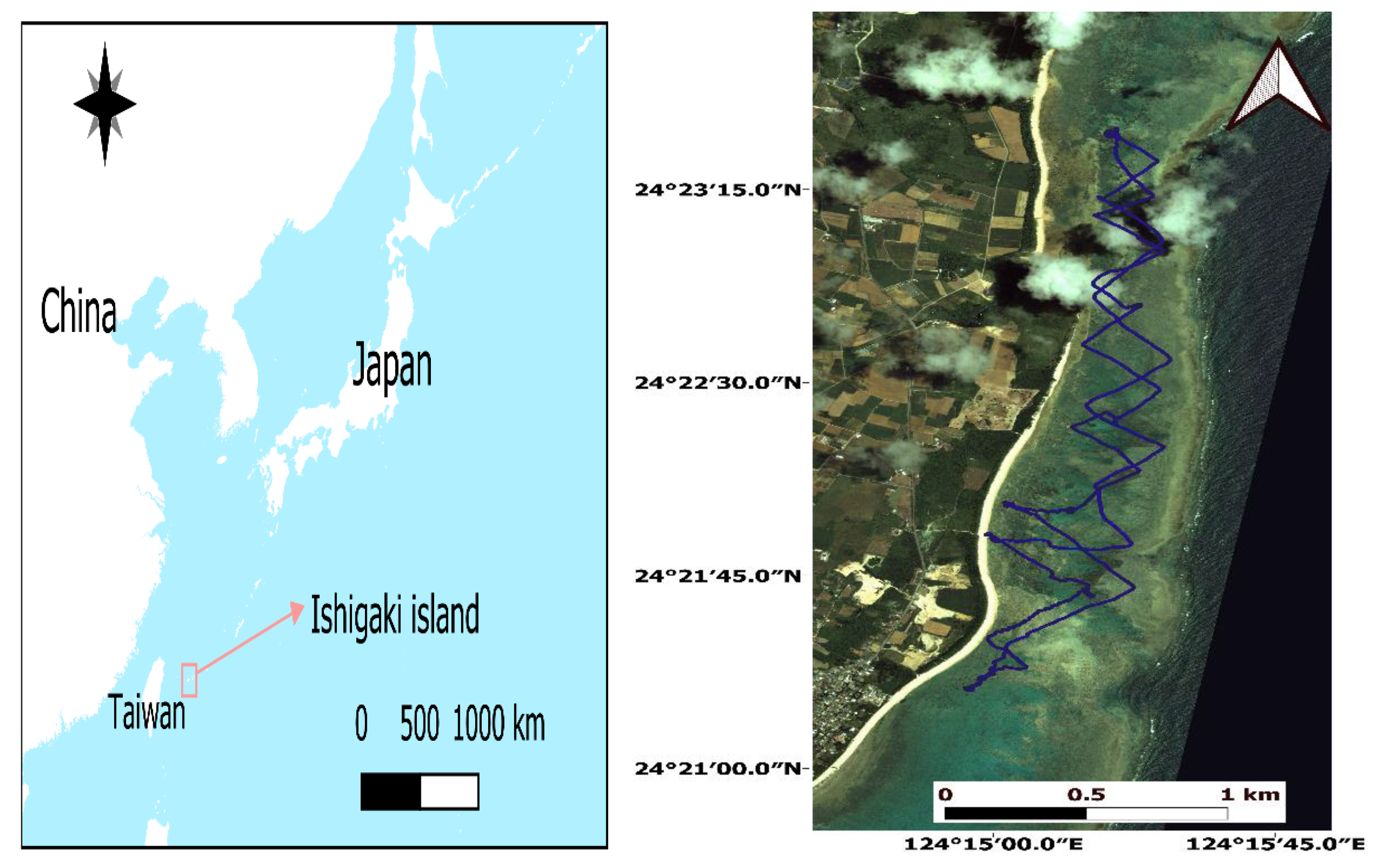
2.1. Study Area

The Shiraho coast subtropical territory, Ishigaki Island, positioned south of Japan in the Pacific Ocean, was the study area chosen for the proposed framework assessment (Figure 1). This Island is rich in marine biodiversity, with shallow, turbid water, and a maximum water depth of 3.5 m [38]. Moreover, it has a heterogeneous ecosystem with various reefscapes, including hard corals, such as Acropora spp., Montipora spp., and Porites cylindrica, and blue corals, such as Heliopora coerulea, considered the largest blue ridge coral colony in the northern hemisphere. It also has a wide range of brown and other algae, as well as a variety of sediments (mud, sand, and boulders). Further, a dense Thalassia hemprichii seagrass meadow spreads across the same seafloor.

2.2. Benthic Cover Field Data Collection

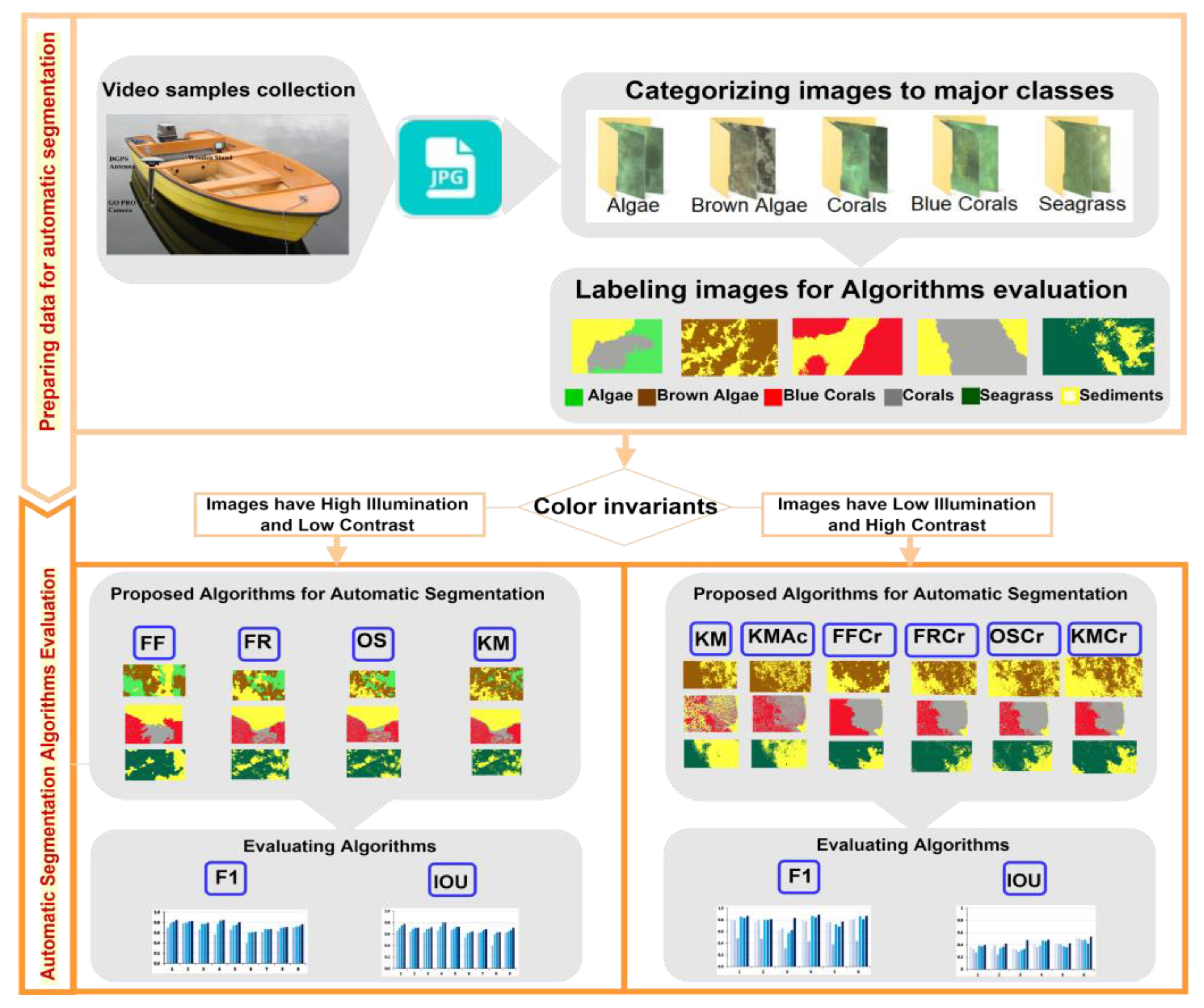
Field data collection in the study area was performed during the typhoon season on 21 August 2016. Outflows from the Todoroki River tributary to the Shiraho reef were boosted by rainstorms before data acquisition. These outflows increased turbidity in underwater images obtained using a low-cost, high-resolution towed video camera (GoPro HERO3 Black Edition) [39]. The video camera was attached beneath the motorboat side just under the water surface to record shallow seabed images. Four hours of recordings were collected and video to JPG converter software was used to extract images from video files. The extracted images had two-second time intervals synchronized with GNSS surveys.

2.3. Methodology

The proposed framework for benthic habitat automatic segmentation over the Shiraho area was performed as:

• All images from the video to JPG converter program were divided into five benthic cover datasets with dominant habitats—brown algae, other algae, corals (Acropora and Porites), blue corals (H. coerulea), seagrass, and the sediments (mud, sand, pebbles, and boulders)—included in all images.
• A total of 125 converted images were selected individually by an expert and divided equally to represent the above benthic cover categories.
• These images included all challenging variations in the underwater images, including poor illumination, blurring, shadows, and differences in brightness.
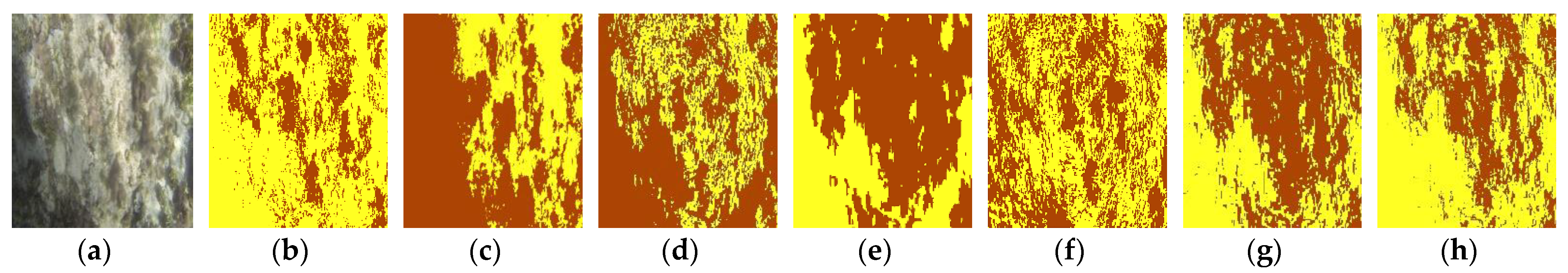
• A manual digitizing was applied carefully for these images. Each image displayed two or three categories, converted to raster form using ARC GIS software.
• Manually categorized images were reviewed by two other experts. These experts compared manually categorized images to original images to guarantee correctness before evaluating proposed methods.
• A color invariant (shadow ratio) detection equation [40] using the ratio between blue and green bands was used to separate images automatically.
• RGB color space images that showed positive and negative values, indicating high illumination, low brightness variation, and no shadow effects, were used for segmentation.
• Otherwise, RGB color space images with only negative values, indicating low illumination, high brightness variation, and shadow effects, were converted to (CIE) LAB and YCbCr color spaces before segmentation.
• The Cr band from YCbCr color spaces represents the difference between the red component and a reference value, and the Ac band from (CIE) LAB color spaces represents the magnitude of red and green tones. Converted images were used for segmentation.
• Proposed unsupervised algorithms were assessed for segmentation and compared to manually categorized images.

2.4. Proposed Unsupervised Algorithms for Automatic Benthic Habitat Segmentation

2.4.1. K-Means Algorithm

KM clustering is a classical unsupervised segmentation algorithm. This algorithm is simple, fast, easy to implement, and efficient and can be applied to large datasets [41]. The algorithm works by partitioning a dataset into k clusters, pre-defined by users [42]. Euclidean distance is used to compare distances between features and cluster centers and assigns each feature to the nearest center [43]. Then, variance is used to remove outlier pixels and regions with an object remover technique after segmentation. Finally, a median filter is applied to remove noise from segmented images [44]. KM algorithm steps were previously described [45].

2.4.2. Otsu Algorithm

The OS method is a straightforward, stable, and effective threshold-based segmentation algorithm widely used for image processing applications [46]. Initially, a greyscale histogram is used to divide the image into two classes—background and target objects [47,48]. Next, an exhaustive search selects an optimal threshold that maximizes separability and minimizes variance within classes. This threshold is the weighted sum of variances of background and target classes [49]. Processing steps for the OS method were also previously described [48].

2.4.3. Fast and Robust Fuzzy C-Means Algorithm

Fuzzy C-means (FCM) [45] is a soft clustering method that depends on the fuzziness value concept and removing conditions. Each pixel may be included in two or more clusters with various degrees of membership ranging between 0 and 1 [50]. Each objective function can be described by distance aggregates between patterns and cluster centers. However, this method yielded poor results if analyzed images included outliers, noise, and imaging artifacts [51]. Thus, an FR algorithm [52] was developed to overcome the limitations of the FCM method. FR applied a morphological reconstruction operation to integrate local spatial information into images. Membership separation was also modified using local membership filtering based on spatial neighbors of the membership divide [53]. These amendments improved algorithm celerity, robustness, and efficiency.

2.4.4. Superpixel-Based Fast Fuzzy C-Means Algorithm

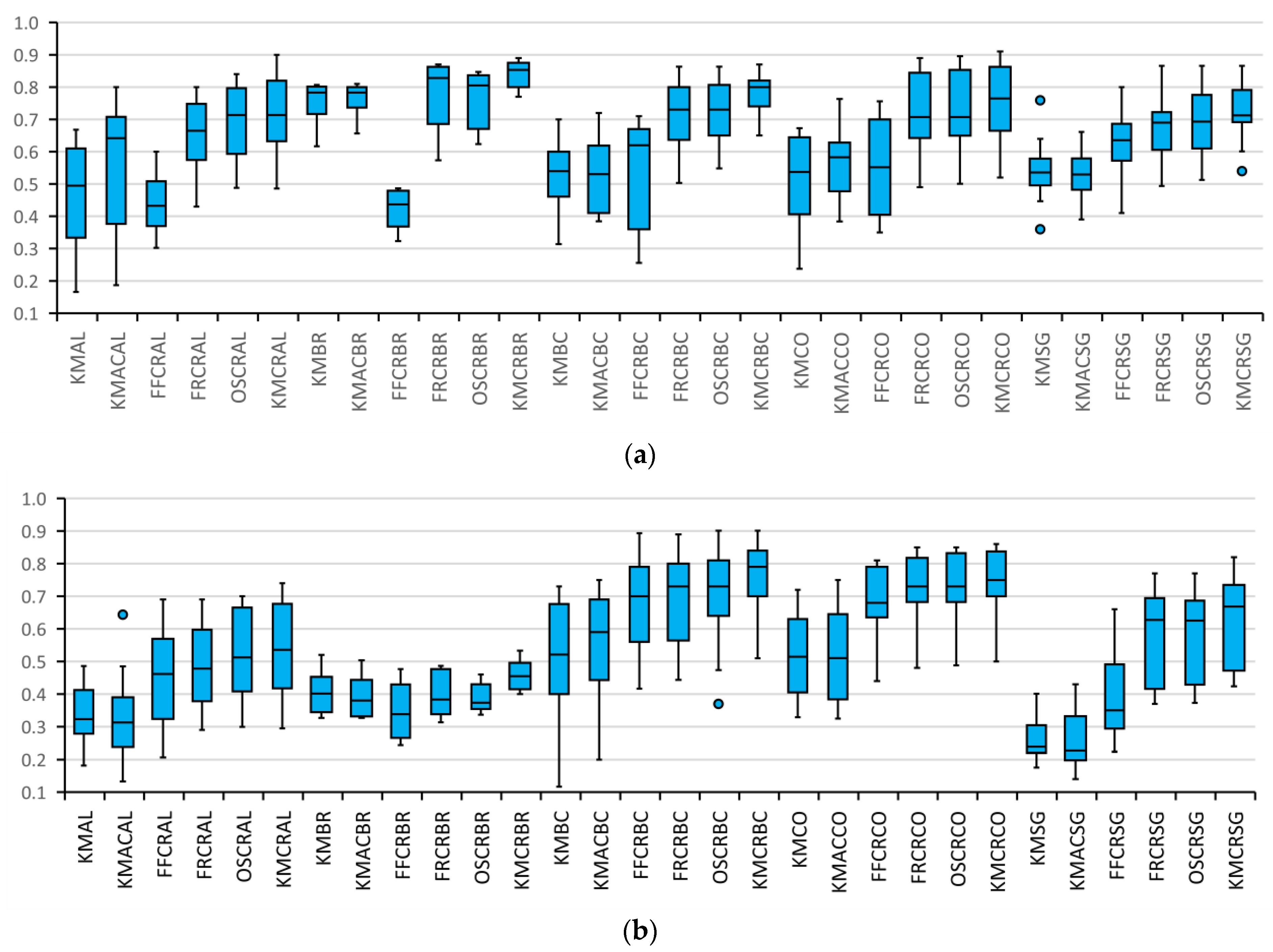
The FF algorithm [54] was proposed to improve the FCM method, particularly its computational complexity and time consumption. FF uses a morphological gradient reconstruction process to generate superpixel images. This approach is more helpful for color image segmentation. The image histogram is then computed for the produced superpixel image. Finally, the FCM method was applied using histogram parameters to produce the final segmentation [55]. The proposed algorithm is more robust and faster than the conventional FCM and yields better results for color image segmentation.

Numerous studies are available for comparing KM, OS, and FCM methods. These studies illustrate the drawbacks of OS and FCM methods and support a preference for the KM approach [56,57,58]. The OS method is a global thresholding algorithm that depends on pixel grey values, while KM is a local thresholding method. Moreover, the OS method must compute a greyscale histogram before running, and KM does not require this step. Furthermore, the OS method produced good results only if the image histogram was not affected by image noise and had a bimodal distribution [59]. Consequently, KM is faster, more efficient, avoids image noise, and can be enhanced to multilevel thresholding [57].

FCM requires various fuzzy calculations and iterations that increase its complexity and computation time compared to KM. Further, FCM is sensitive to noise, unlike KM clustering. Hassan et al. [60] discussed the differences between KM and FCM.

All benthic cover unsupervised segmentation algorithms were applied in the MATLAB environment with pre-defined numbers of clusters. The assessment of all algorithms depended on two matrices normally used for segmentation evaluation—Intersection Over Union (IOU) and F1 − score (F1) [18]:

$$\mathrm{IOU}=\frac{\mathrm{True} \mathrm{Positives}}{\mathrm{True} \mathrm{Positives} + \mathrm{False} \mathrm{Positives} + \mathrm{False} \mathrm{Negatives}}$$

(1)

$$\mathrm{F}1-\mathrm{score}=\frac{2\times \mathrm{Precision}\times \mathrm{Recall}}{\mathrm{Precision} + \mathrm{Recall}}$$

(2)

The procedures for automatic benthic habitat segmentation methods are shown in Figure 2.

3. Results

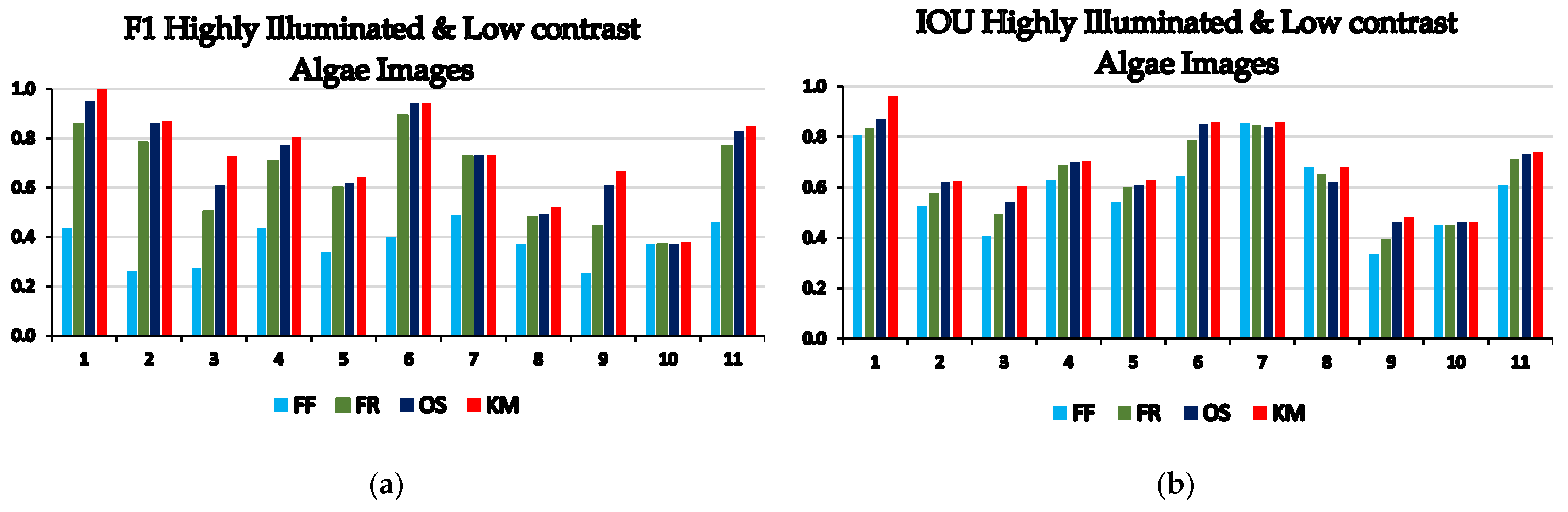
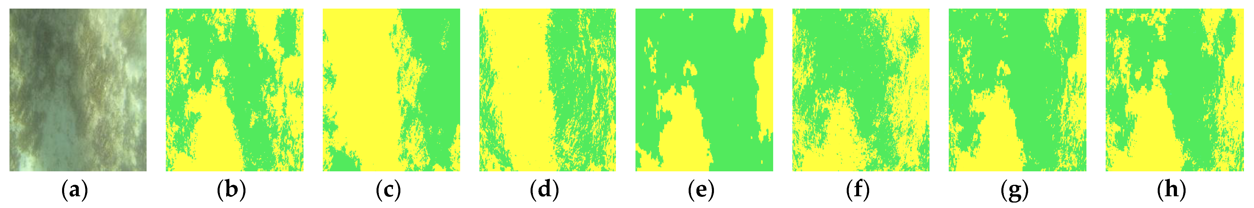
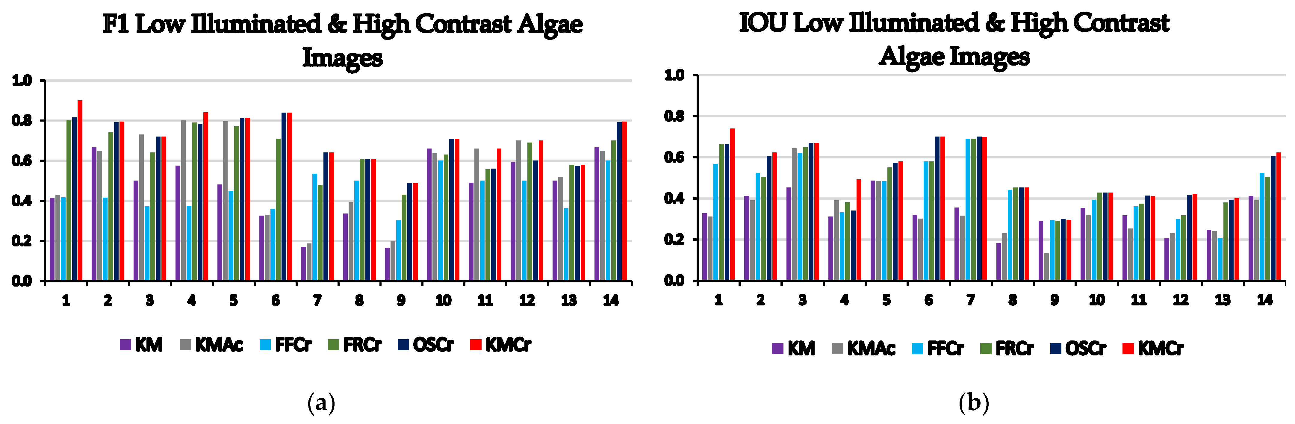
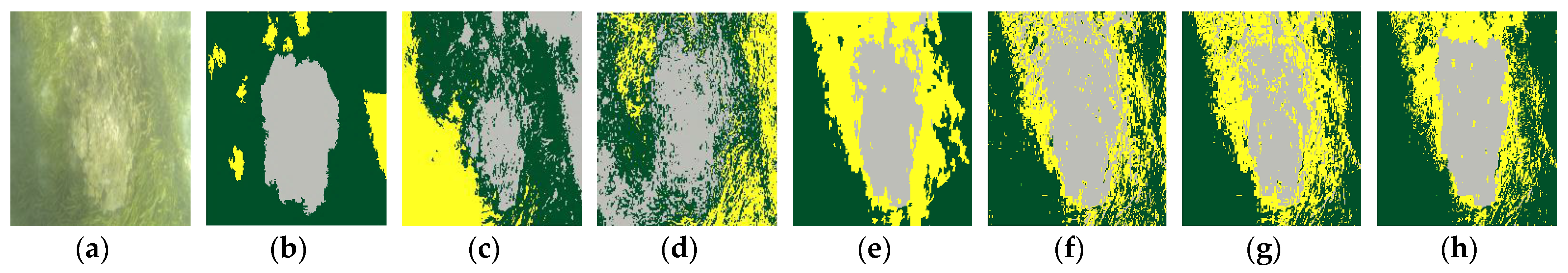
3.1. Results of Automatic Segmentation of Algal Images

The comparison of segmentation methods for both highly illuminated and low contrast algal images and poorly illuminated and high contrast algal images are presented in Figure 3 and Figure 4, respectively. Examples of classified images with two and three categories are presented in Figure 5, Figure 6, Figure 7 and Figure 8.

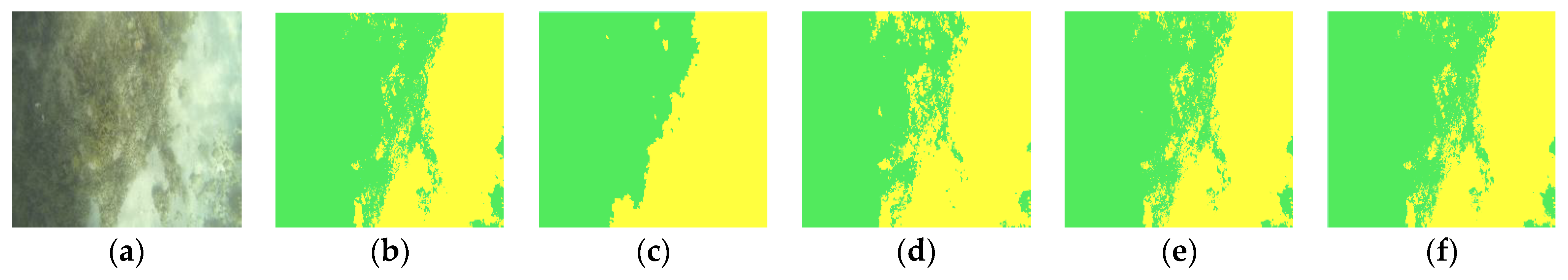
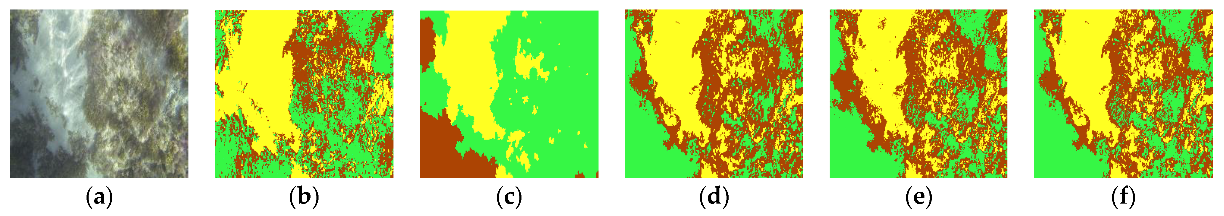
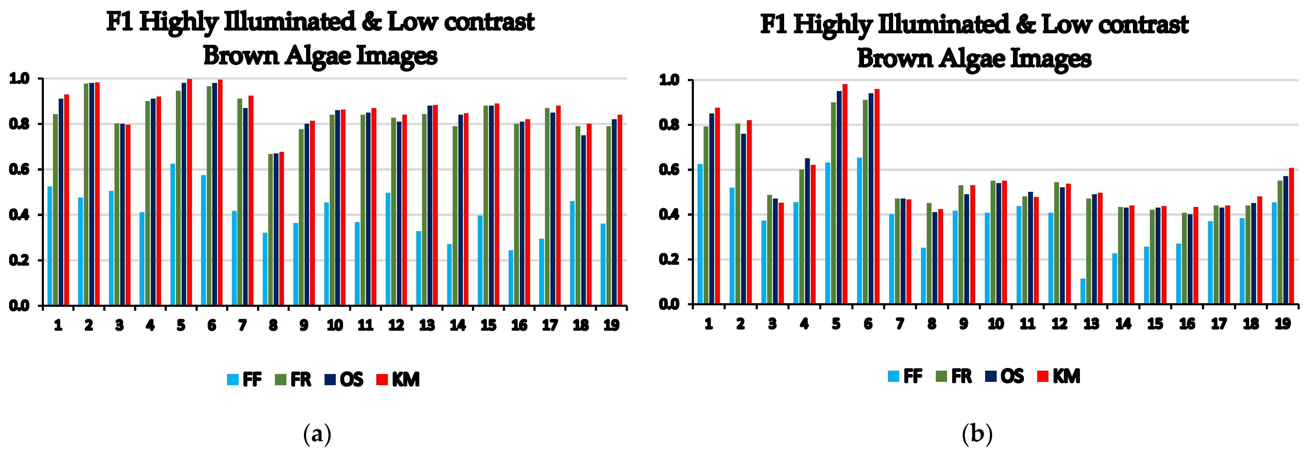
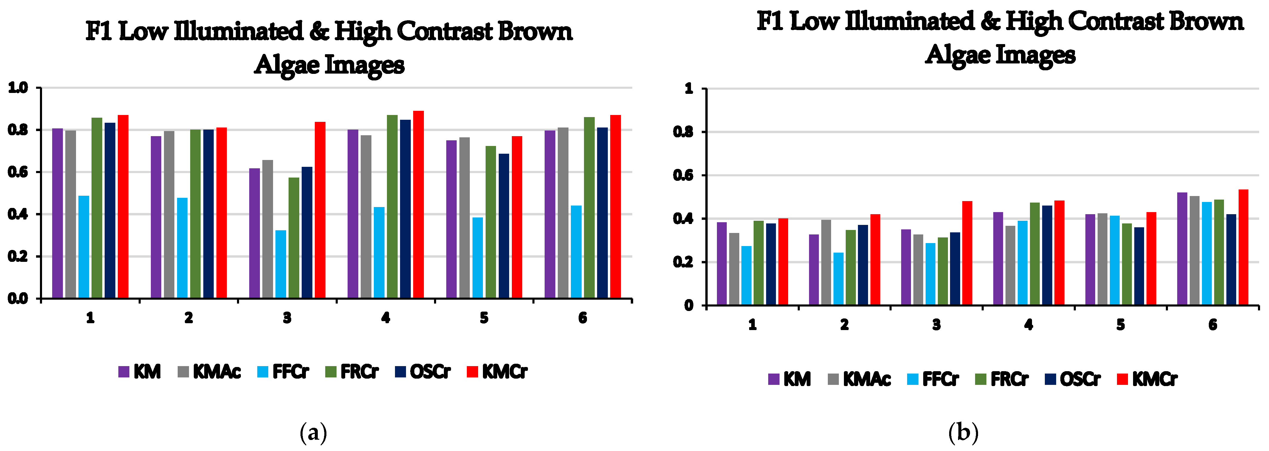
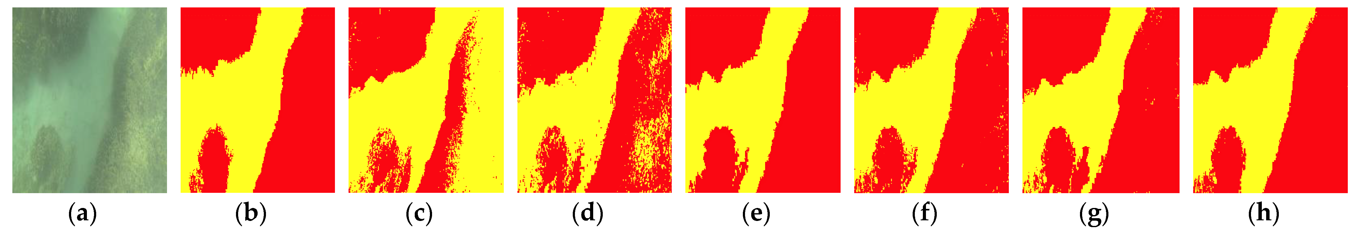
3.2. Results of Automatic Segmentation of Brown Algae Images

The comparisons of segmentation methods for both highly illuminated and low contrast brown algae images and poorly illuminated and high contrast brown algae images are presented in Figure 9 and Figure 10, respectively. Examples of classified images with two and three categories are presented in Figure 11, Figure 12, Figure 13 and Figure 14.

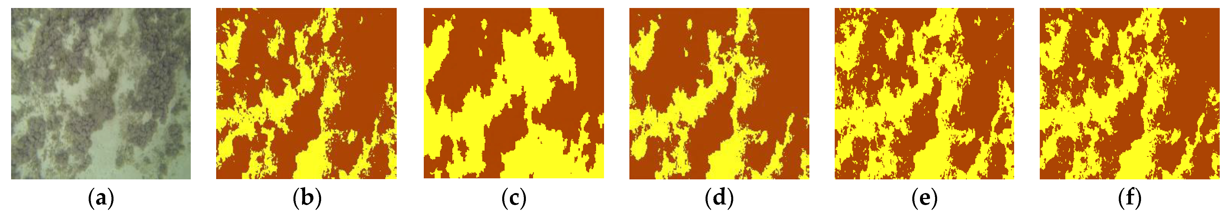
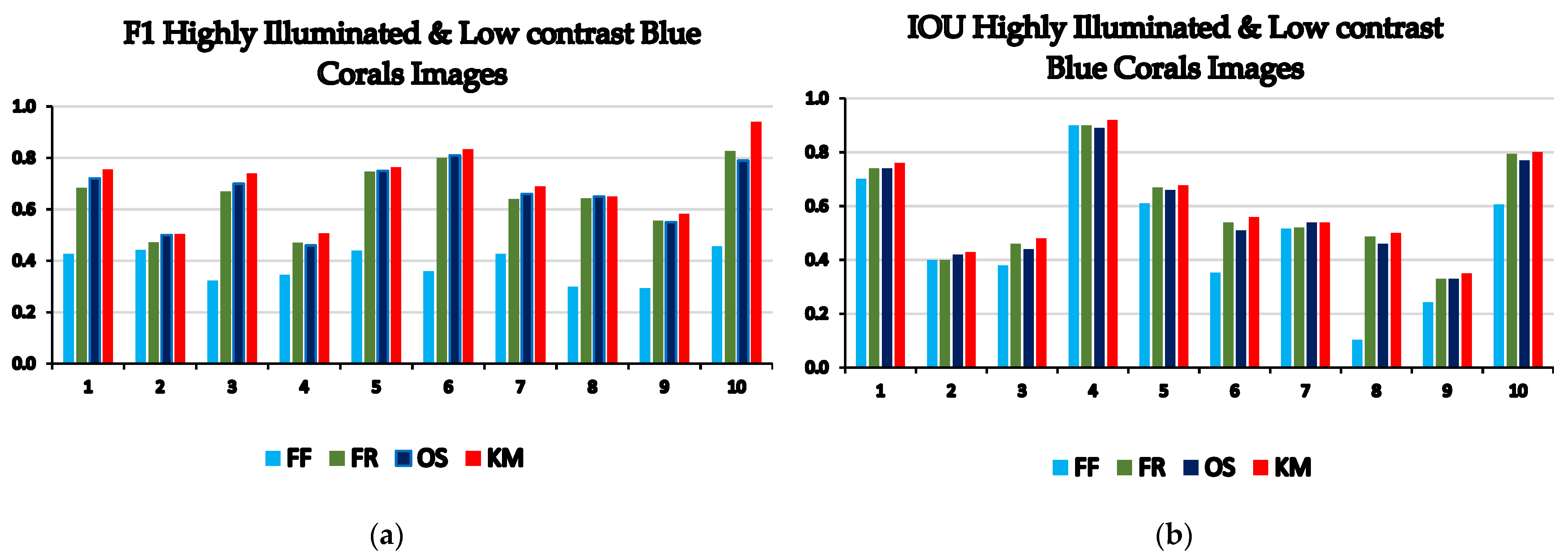
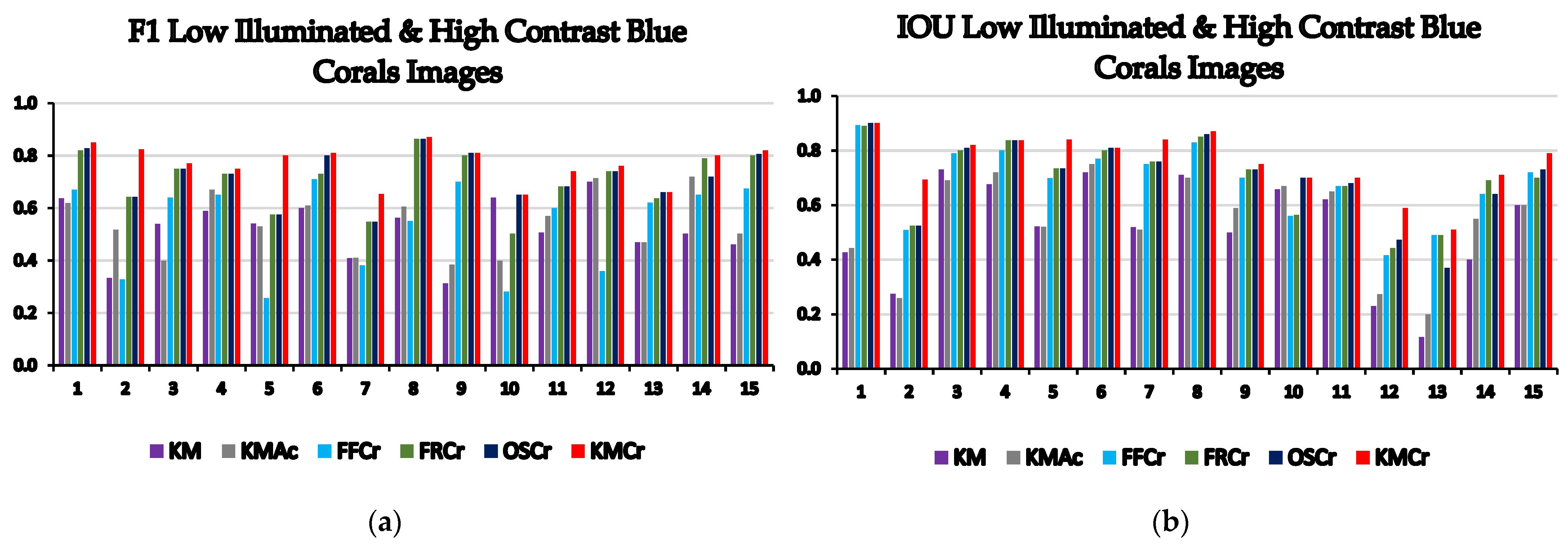
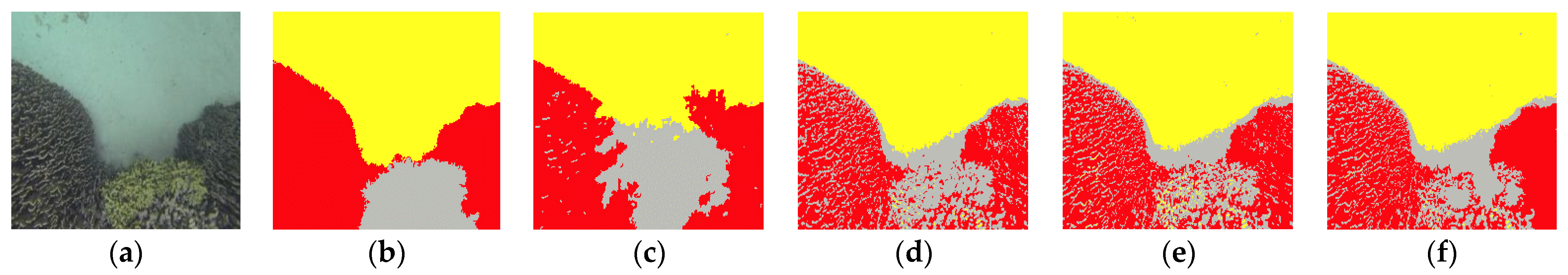
3.3. Results of Automatic Segmentation of Blue Coral Images

The comparisons of segmentation methods for both highly illuminated and low contrast blue coral images and poorly illuminated and high contrast blue coral images are presented in Figure 15 and Figure 16, respectively. Examples of classified images with two and three categories are presented in Figure 17, Figure 18, Figure 19 and Figure 20.

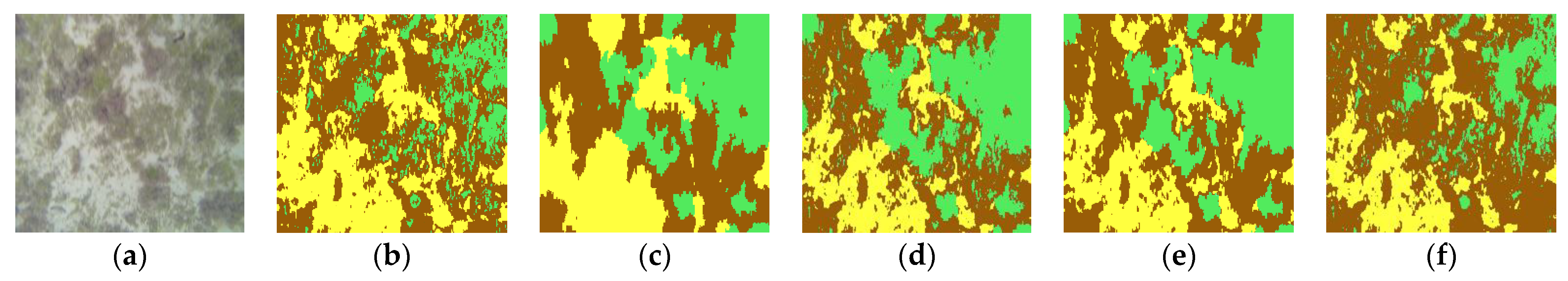
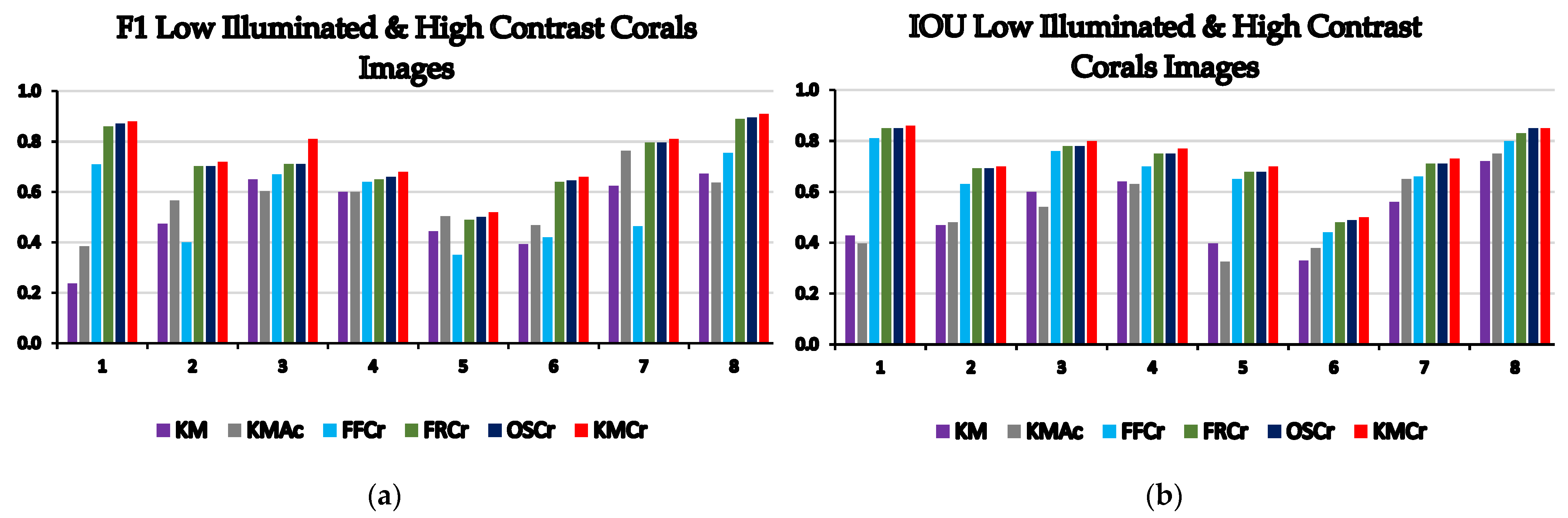
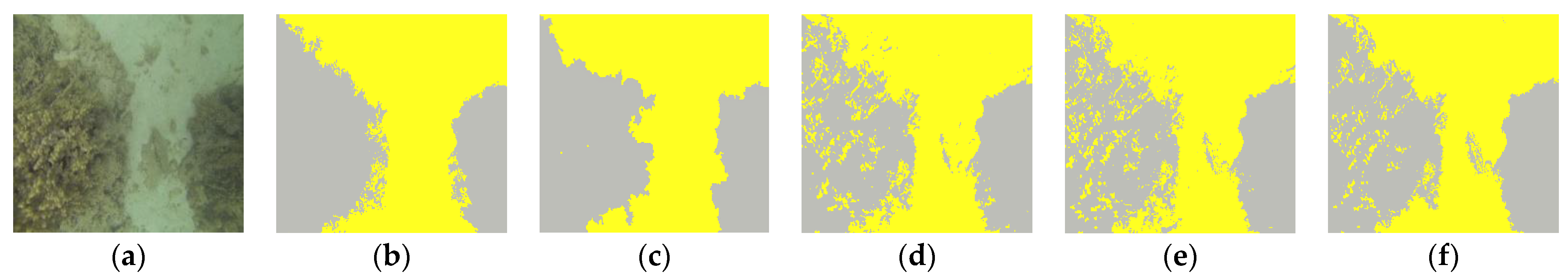
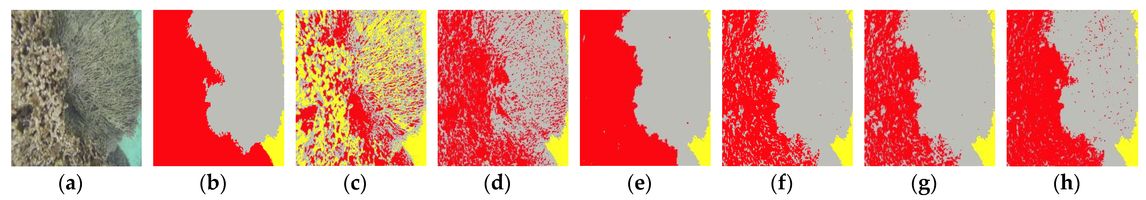
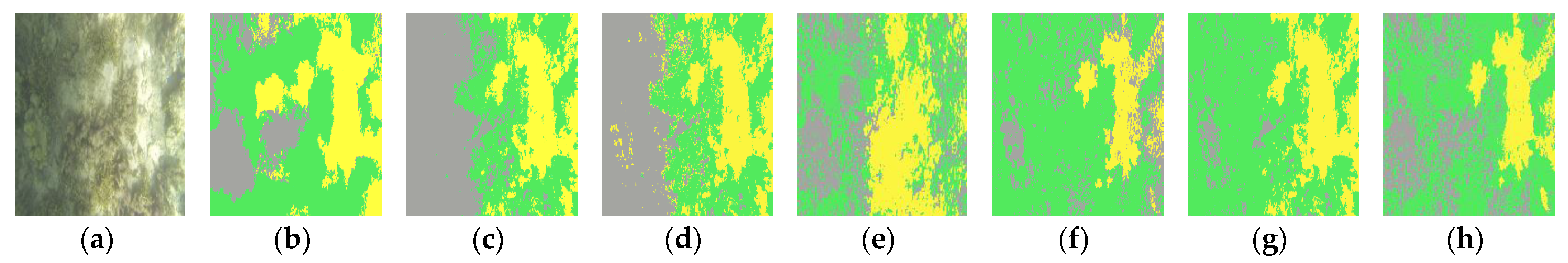
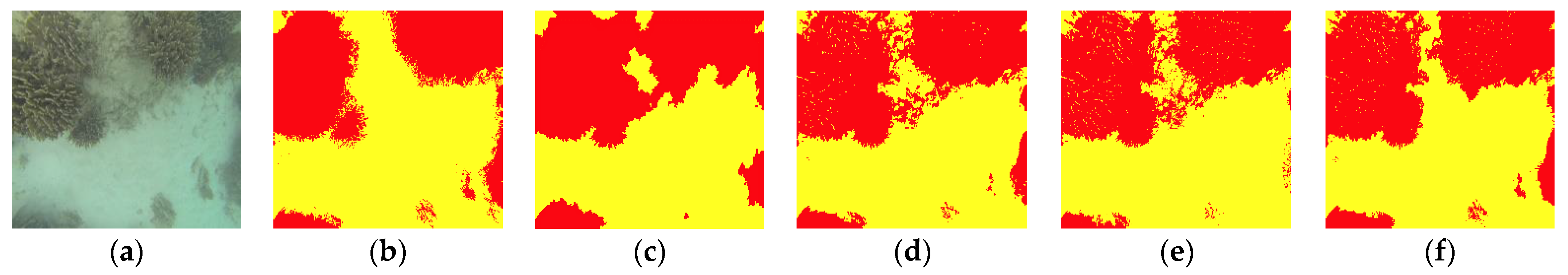
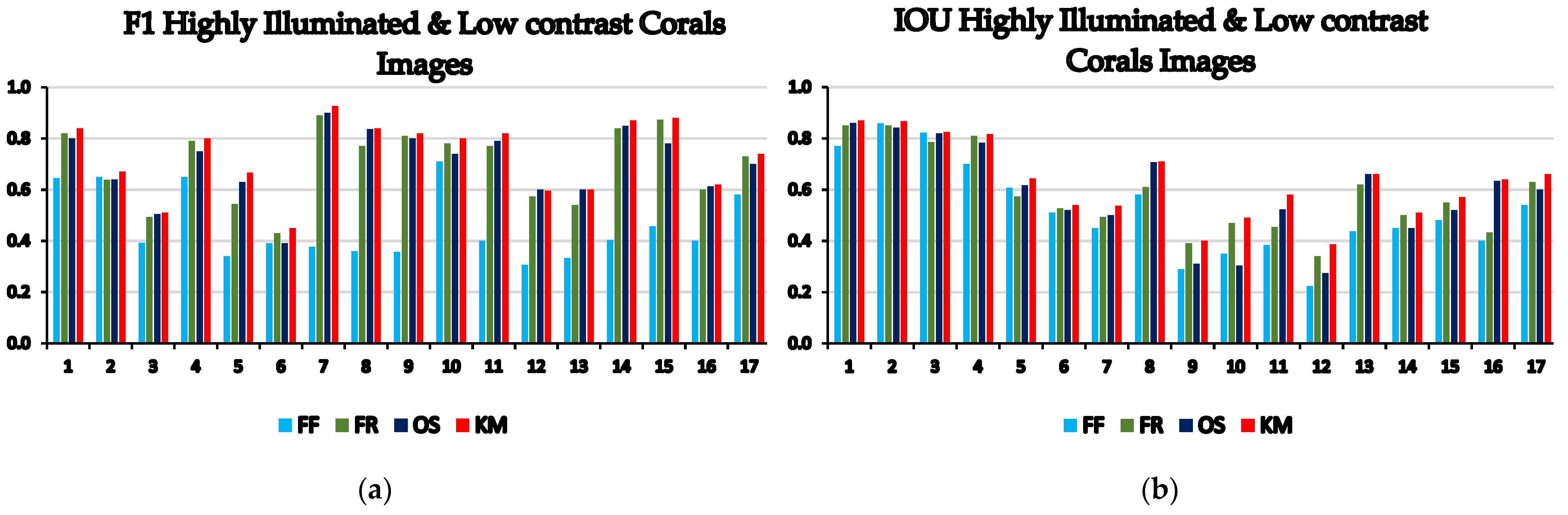
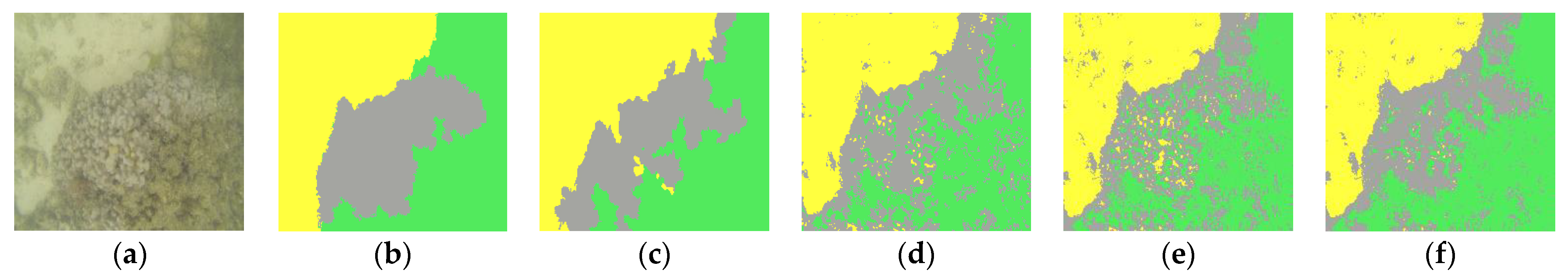
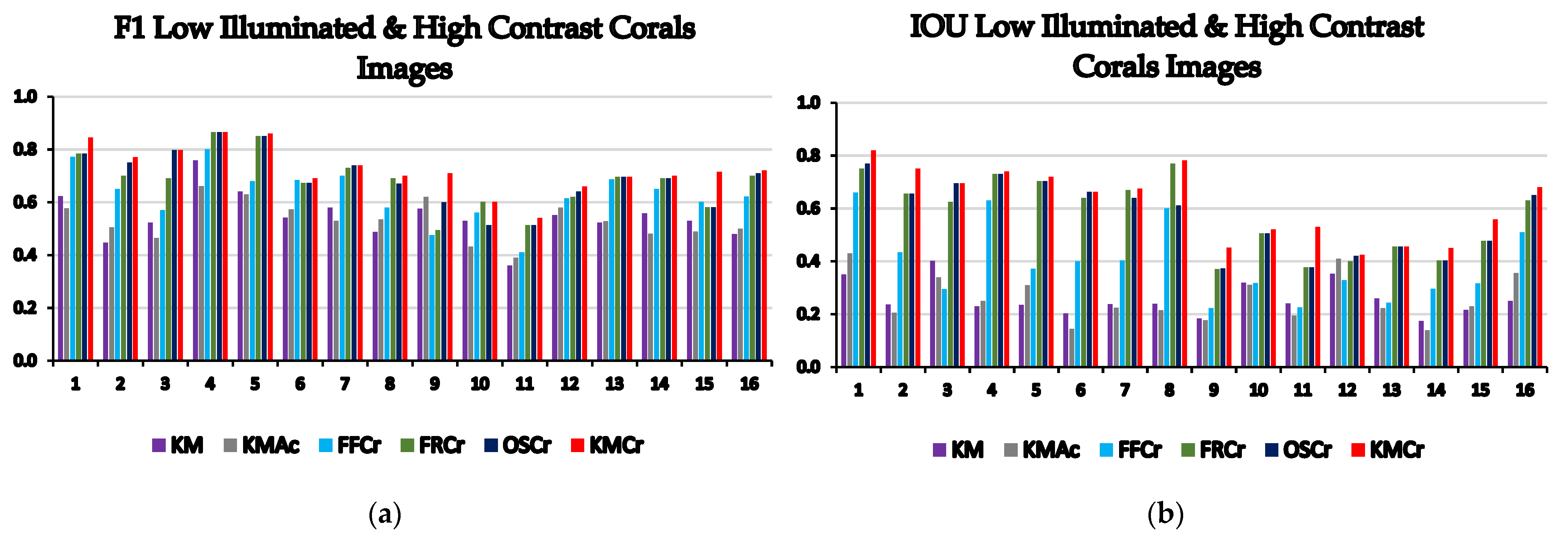
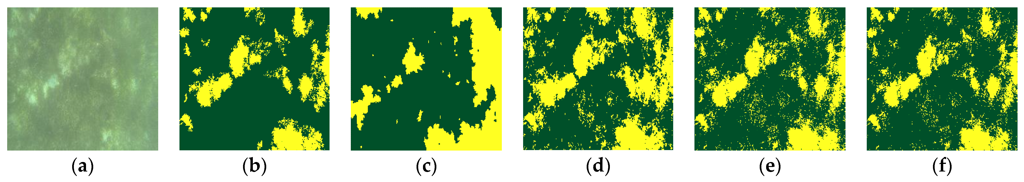
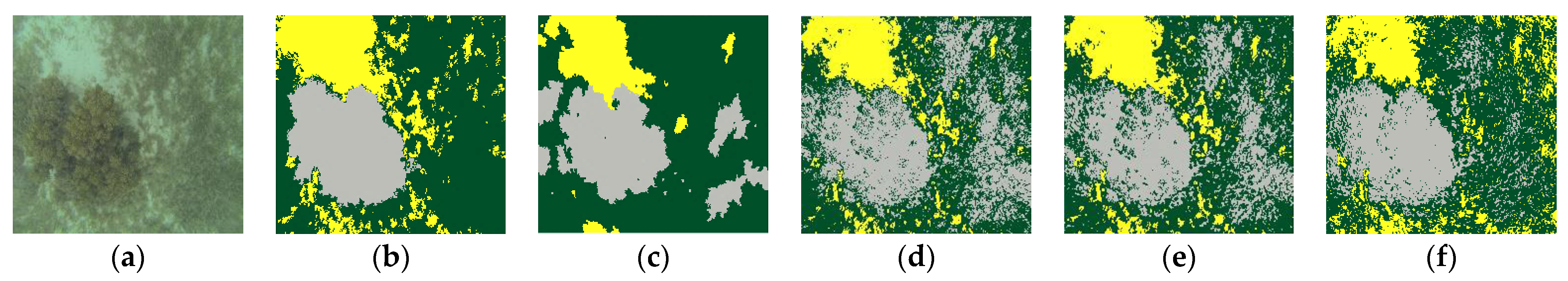
3.4. Results of Automatic Segmentation of Coral Images

The comparisons of segmentation methods for both highly illuminated and low contrast coral images and poorly illuminated and high contrast coral images are presented in Figure 21 and Figure 22, respectively. Examples of classified images with two and three categories are presented in Figure 23, Figure 24, Figure 25 and Figure 26.

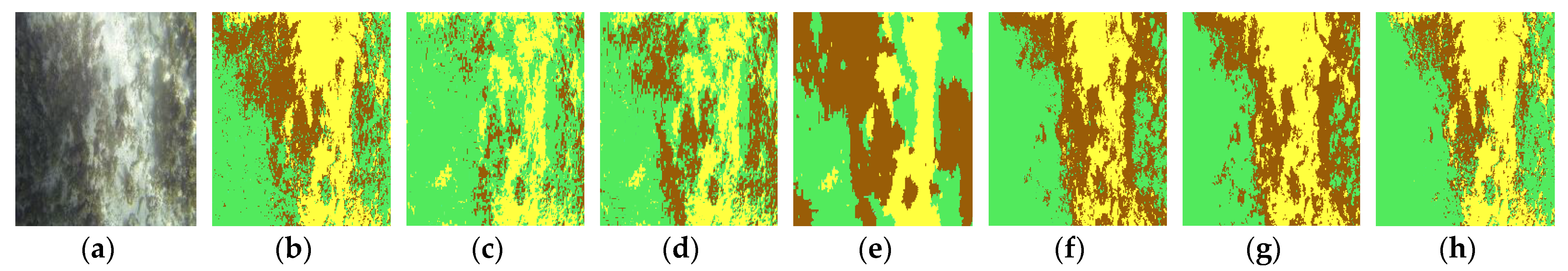
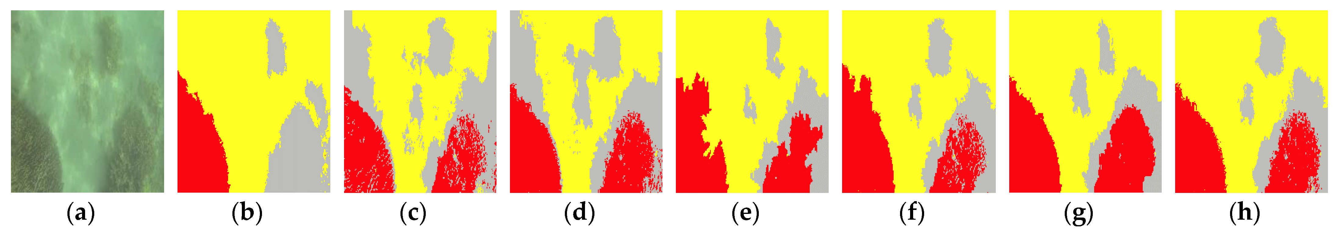
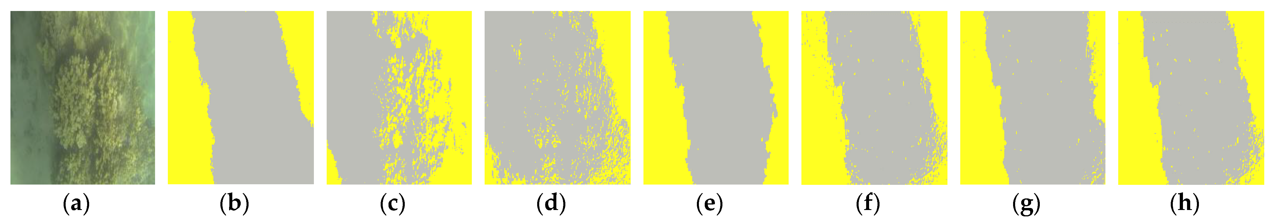
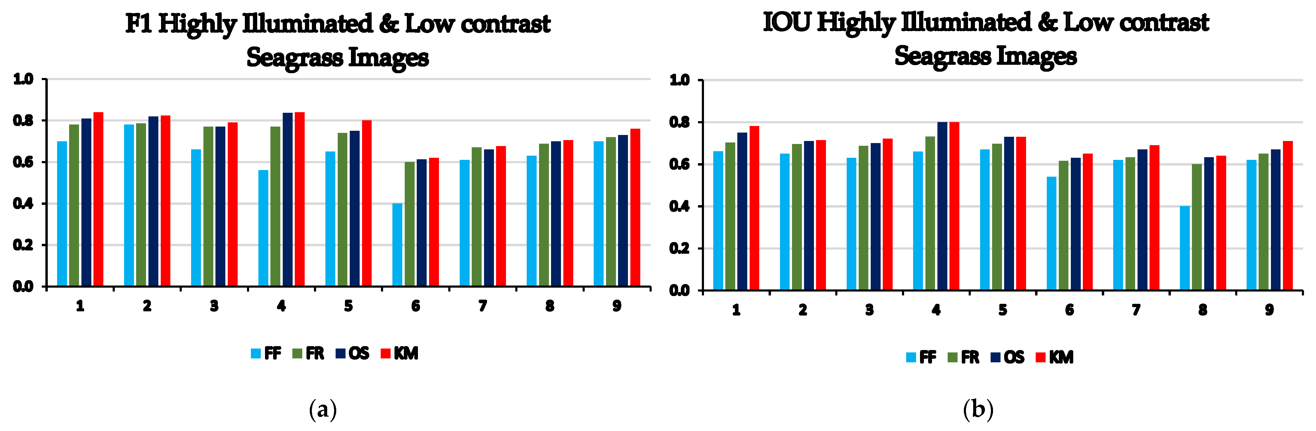
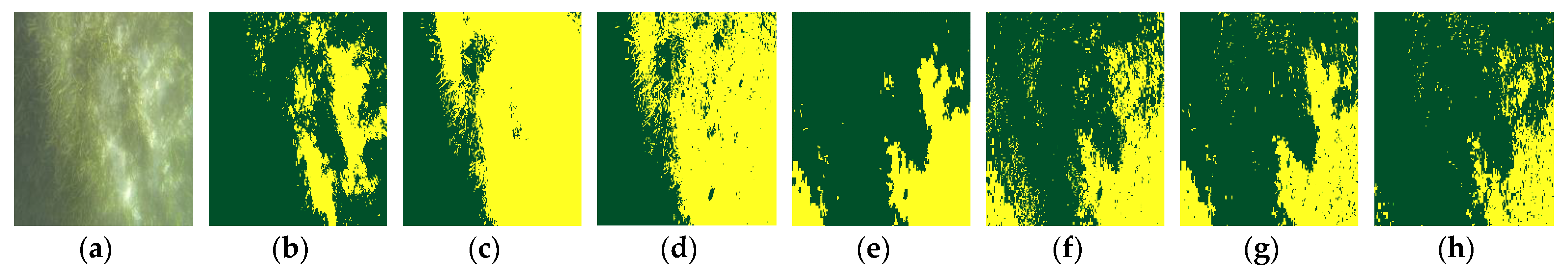
3.5. Results of Automatic Segmentation of Seagrass Images

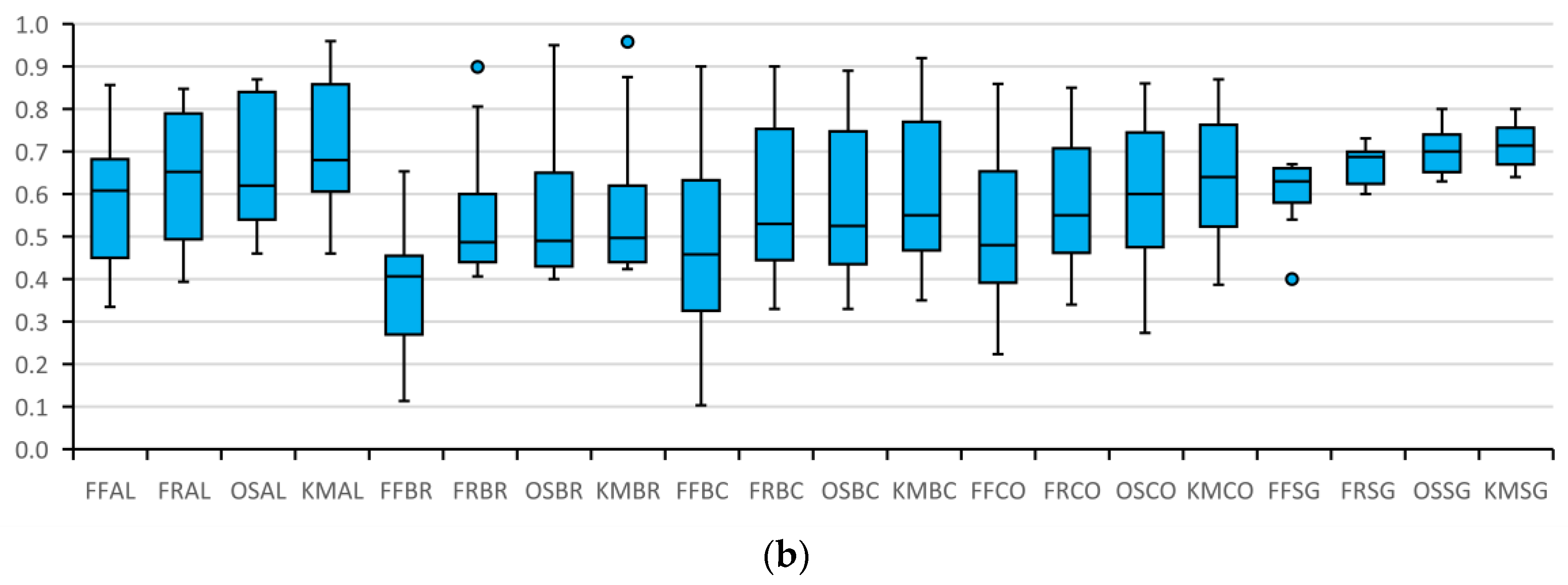
The comparisons of segmentation methods for both highly illuminated and low contrast seagrass images and poorly illuminated and high contrast seagrass images are presented in Figure 27 and Figure 28, respectively. Examples of classified images with two and three categories are presented in Figure 29, Figure 30, Figure 31 and Figure 32.

Results presented in Figure 33 and

Table 1. The average F1-Score and IOU results of the proposed algorithms on the tested highly illuminated and low contrast benthic habitat images.

Benthic Habitat	F1-FF	F1-FR	F1-OS	F1-KM	IOU-FF	IOU-FR	IOU-OS	IOU-KM
AL	0.37	0.65	0.71	0.74	0.59	0.64	0.66	0.69
BR	0.41	0.85	0.86	0.87	0.40	0.56	0.57	0.58
BC	0.38	0.65	0.66	0.70	0.48	0.58	0.58	0.60
CO	0.46	0.70	0.70	0.73	0.52	0.58	0.58	0.63
SG	0.63	0.72	0.74	0.76	0.61	0.67	0.70	0.72

correspond to results in Figure 3, Figure 9, Figure 15, Figure 21 and Figure 27. Figure 33 illustrates overall accuracy for highly illuminated and low contrast images, and Table 1 shows F1-Scorse and IOU results. Results in Figure 34 and

Table 2. The average F1-Score and IOU results of the proposed algorithms on the tested low illuminated and high contrast benthic habitat images.

Benthic Habitat	F1 KM	F1 KMAc	F1 FFCr	F1 FRCr	F1 OSCr	F1 KMCr	IOU KM	IOU KMAc	IOU FFCr	IOU FRCr	IOU OSCr	IOU KMCr
AL	0.47	0.55	0.45	0.65	0.70	0.72	0.33	0.33	0.45	0.48	0.52	0.54
BR	0.76	0.77	0.42	0.78	0.77	0.84	0.41	0.39	0.35	0.40	0.39	0.46
BC	0.52	0.54	0.54	0.71	0.72	0.77	0.51	0.54	0.68	0.70	0.70	0.76
CO	0.51	0.57	0.55	0.72	0.72	0.75	0.52	0.52	0.68	0.72	0.72	0.74
SG	0.54	0.53	0.63	0.68	0.69	0.73	0.26	0.26	0.39	0.57	0.57	0.62

correspond to results in Figure 4, Figure 10, Figure 16, Figure 22 and Figure 28. Figure 34 shows overall accuracy for poorly illuminated and high contrast images, and Table 2 presents F1-Scores and IOU values.

Table 3. Comparison of statistically significant differences in F1-Score and IOU results between the proposed algorithms with a confidence of 95%.

Comparison Test	p-Value t-Test F1	p-Value Wilcoxon Test F1	p-Value t-Test IOU	p-Value Wilcoxon-Test IOU	Comparison Results
KM vs. OS	0.03 (h = 1)	0.051 (h = 0)	0.127 (h = 0)	0.154 (h = 0)	Not significantly different
KM vs. FR	0.006 (h = 1)	0.004 (h = 1)	0.037 (h = 1)	0.042 (h = 1)	Significantly different
KM vs. FF	<0.001 (h = 1)	<0.001 (h = 1)	<0.001 (h = 1)	<0.001 (h = 1)	Significantly different

illustrates the evaluation of the statistical significance of differences between the tested algorithms.

4. Discussion

Benthic habitat surveys using towed cameras attached beneath motorboats have several advantages. First, this approach can cover large habitat areas without environmental damage. Second, the system requires only simple logistics and is economical, which increases its utility for marine applications. Third, it can be used to monitor changes in heterogeneous ecosystems annually. However, such surveys are performed under inadequate natural lighting conditions that affect image quality. Thus, segmentation algorithms need to overcome the influence of varying light and shadow.

We assessed several color spaces to eliminate the influence of varying illumination and shadows on survey images. Images were converted to color spaces, and color information was separated from luminance or brightness of images. This process decreased the impact of brightness variation on segmentation. Both Hue Saturation Value (HSV) and (CIE) XYZ color spaces were assessed for removing illumination effects. However, these color spaces yielded significantly lower F1-scores and IOU segmentation accuracies. However, the Cr band from YCbCr and the (Ac) band from (CIE) LAB color space outperformed other tested color spaces. The Cr band achieved the highest F1-scores and IOU segmentation accuracy. Segmentation results of the KM method RGB color space were added to the assessment to demonstrate the importance of using color spaces for images with variable lighting.

The reason that red-green bands outperform in processing underwater images from coastal areas is often due to agricultural runoff or impurities discharged from rivers. Therefore, both short and long wavelengths are attenuated to some extent. In these areas, blue and green wavelengths are absorbed more efficiently, leaving more red light that causes a brown hue [5]. Moreover, the common notion that red color is attenuated by water more rapidly with depth than blue and green colors only holds for oceanic waters [61].

Pixel, color, thresholding, and region-based segmentation techniques with different architectures were tested in the present study for unsupervised benthic habitat segmentation. Mean shift [62], Normalized Cut [63], Efficient graph-based [64], Ratio-contour [65], Expectation-Maximization [66], and Slope Difference Distribution [67] methods have also been evaluated. However, these latter methods yield relatively low F1-scores and IOU segmentation accuracy values.

Complete comparisons among the evaluated algorithms show maximum, minimum, and median values for tested algorithms in box plots (Figure 33 and Figure 34). The KM method produced the highest segmentation accuracies for all categories. Lower accuracy was found for OS, FR, and FF methods, in that order. Additionally, we tried to integrate KM, OS, and FR segmentation algorithms, but this ensemble produced an accuracy that was similar to the k-means segmentation algorithm alone. The ensemble only increased segmentation accuracy slightly for a few images. Therefore, results from integrated algorithms are not presented.

Moreover, to evaluate the statistically significant differences between the proposed algorithms, the parametric paired t-test and its non-parametric alternative Wilcoxon test [68] were performed. We assessed whether the statistical differences in F1-score and IOU values between the tested approaches were significant or not. Both tests had two output values, the p-value and the h value. The p-value indicated the significance of the statistical null hypothesis test. Small p-values mean strong proof against the null hypothesis. The h value is the hypothesis test result returned as 1 or 0. If the resulted h value was 1, the null hypothesis test was rejected. This indicates a statistically significant difference between the compared algorithms and 0 otherwise. Overall, non-parametric tests are stronger and safer than parametric tests, particularly when comparing a pair of algorithms [69].

As the KM method yielded the highest F1-score and IOU accuracies, we compared the other proposed algorithms against the KM method in order to test whether the F1-score and IOU results were significantly different between the compared methods (Table 3). Based on the F1-score results, the paired t-test indicated a significant difference between the KM and OS methods. Conversely, the Wilcoxon test p-value result was slightly greater than the 0.05 significance level. As a result, the Wilcoxon test failed to reject the null hypothesis test and indicated no statistically significant difference between these methods. Moreover, based on the paired t-test and Wilcoxon test, there was no significant difference between the IOU results of KM and OS methods at the 5% significance level. On the other hand, the KM algorithm was significantly different from both FR and FF algorithms.

We assessed various benthic images with different light conditions, species diversity, and turbidity levels to avoid statistical bias. In the majority of images, the brown algae and the other algae were mixed in the same locations as were blue corals and other corals, which confused all algorithms. The most challenging segmentation task was discriminating among brown algae, other algae, and sediments. All of these habitat types display small-sized objects and similar speckled shapes (see Figure 14). Thus, brown algae and other algae, especially in poorly illuminated images, yielded the lowest IOU segmentation accuracy (see Figure 34). Discriminating blue coral segments from other coral species was also challenging because corals exhibit similar colors and shapes (see Figure 20). Conversely, the seagrass habitat was categorized with high accuracy. Considering species heterogenicity and the poor quality of tested images, accuracies obtained in the present study can be considered reliable for automatic benthic habitat segmentation. Note that comparing our segmentation accuracies with previous studies is difficult due to differences in the quality of images used, water turbidity levels in various locations, and the variety of substrates.

These automatic segmentation results encourage more research in this field. Such studies might assess the same methods with remotely operated vehicle (ROV) systems with auxiliary light sources for monitoring benthic habitats in deeper seafloor areas. The additional light source will increase image quality and segmentation accuracy. Additionally, segmentation algorithms that can decrease light variation and shadow effects [70,71] might be evaluated with the same poor-quality images. Finally, segmentation techniques can be evaluated with more complex habitat images for the same targets.

Conversely, assessing the performance of deep learning algorithms trained by the segmented images might lead to more robust benthic habitat monitoring systems. Integrating automatically segmented images with known segmented locations might allow classifying satellite images over coral reef areas.

5. Conclusions

This study used images from a towed underwater camera to evaluate the performance of unsupervised segmentation algorithms for automatic benthic habitat classification. Moreover, we assessed various color spaces to remove illumination variation and shadow effects from poor-quality images. The Shiraho coastal area, which includes heterogeneous blue corals, corals, algae, brown algae, seagrass, and sediment, was used as a validation site. Our results demonstrate superior performance for the Cr band from the YCbCr color space to remove light variation and shadow effects. Further, we found that the KM segmentation algorithm achieved the highest F1-scores and IOU accuracies for habitat segmentation. The significance testing of the F1-score and IOU statistics revealed that the KM model performed significantly better (at the 5% level) than FR and FF methods. Moreover, a similar performance was found between the KM and OS methods. The proposed automatic segmentation framework is fast, simple, and inexpensive for seafloor habitat categorization. Thus, a large number of benthic habitat images can be accurately categorized with minimal effort.

References

1. Li, A.S.; Chirayath, V.; Segal-Rozenhaimer, M.; Torres-Perez, J.L.; Van Den Bergh, J. NASA NeMO-Net’s Convolutional Neural Network: Mapping Marine Habitats with Spectrally Heterogeneous Remote Sensing Imagery. IEEE J. Sel. Top. Appl. Earth Obs. Remote Sens. 2020, 13, 5115–5133. [Google Scholar] [CrossRef]
2. Mizuno, K.; Terayama, K.; Hagino, S.; Tabeta, S.; Sakamoto, S.; Ogawa, T.; Sugimoto, K.; Fukami, H. An efficient coral survey method based on a large-scale 3-D structure model obtained by Speedy Sea Scanner and U-Net segmentation. Sci. Rep. 2020, 10, 12416. [Google Scholar] [CrossRef] [PubMed]
3. Balado, J.; Olabarria, C.; Martínez-Sánchez, J.; Rodríguez-Pérez, J.R.; Pedro, A. Semantic segmentation of major macroalgae in coastal environments using high-resolution ground imagery and deep learning. Int. J. Remote Sens. 2021, 42, 1785–1800. [Google Scholar] [CrossRef]
4. Gapper, J.J.; El-Askary, H.; Linstead, E.; Piechota, T. Coral reef change detection in remote Pacific Islands using support vector machine classifiers. Remote Sens. 2019, 11, 1525. [Google Scholar] [CrossRef] [Green Version]
5. Pavoni, G.; Corsini, M.; Pedersen, N.; Petrovic, V.; Cignoni, P. Challenges in the deep learning-based semantic segmentation of benthic communities from Ortho-images. Appl. Geomat. 2020, 12, 131–146. [Google Scholar] [CrossRef]
6. Chirayath, V.; Instrella, R. Fluid lensing and machine learning for centimeter-resolution airborne assessment of coral reefs in American Samoa. Remote Sens. Environ. 2019, 235, 111475. [Google Scholar] [CrossRef]
7. Floor, J.; Kris, K.; Jan, T. Science, uncertainty and changing storylines in nature restoration: The case of seagrass restoration in the Dutch Wadden Sea. Ocean Coast. Manag. 2018, 157, 227–236. [Google Scholar] [CrossRef]
8. Piazza, P.; Cummings, V.; Guzzi, A.; Hawes, I.; Lohrer, A.; Marini, S.; Marriott, P.; Menna, F.; Nocerino, E.; Peirano, A.; et al. Underwater photogrammetry in Antarctica: Long-term observations in benthic ecosystems and legacy data rescue. Polar Biol. 2019, 42, 1061–1079. [Google Scholar] [CrossRef] [Green Version]
9. Mizuno, K.; Sakagami, M.; Deki, M.; Kawakubo, A.; Terayama, K.; Tabeta, S.; Sakamoto, S.; Matsumoto, Y.; Sugimoto, Y.; Ogawa, T.; et al. Development of an Efficient Coral-Coverage Estimation Method Using a Towed Optical Camera Array System [Speedy Sea Scanner (SSS)] and Deep-Learning-Based Segmentation: A Sea Trial at the Kujuku-Shima Islands. IEEE J. Ocean. Eng. 2019, 45, 1386–1395. [Google Scholar] [CrossRef]
10. Price, D.M.; Robert, K.; Callaway, A.; Lo lacono, C.; Hall, R.A.; Huvenne, V.A.I. Using 3D photogrammetry from ROV video to quantify cold-water coral reef structural complexity and investigate its influence on biodiversity and community assemblage. Coral Reefs 2019, 38, 1007–1021. [Google Scholar] [CrossRef] [Green Version]
11. Hamylton, S.M. Mapping coral reef environments: A review of historical methods, recent advances and future opportunities. Prog. Phys. Geogr. 2017, 41, 803–833. [Google Scholar] [CrossRef]
12. Mahmood, A.; Bennamoun, M.; An, S.; Sohel, F.; Boussaid, F.; Hovey, R.; Kendrick, G.; Fisher, R.B. Deep Learning for Coral Classification. In Handbook of Neural Computation; Academic Press: Cambridge, MA, USA, 2017; pp. 383–401. ISBN 9780128113196. [Google Scholar]
13. Gómez-Ríos, A.; Tabik, S.; Luengo, J.; Shihavuddin, A.S.M.; Herrera, F. Coral species identification with texture or structure images using a two-level classifier based on Convolutional Neural Networks. Knowl. Based Syst. 2019, 184, 104891. [Google Scholar] [CrossRef] [Green Version]
14. Agrafiotis, P.; Skarlatos, D.; Forbes, T.; Poullis, C.; Skamantzari, M.; Georgopoulos, A. Underwater photogrammetry in very shallow waters: Main challenges and caustics effect removal. In Proceedings of the International Archives of the Photogrammetry, Remote Sensing and Spatial Information Sciences—ISPRS Archives, Riva del Garda, Italy, 4–7 June 2018; Volume XLII–2, pp. 15–22. [Google Scholar]
15. Mahmood, A.; Ospina, A.G.; Bennamoun, M.; An, S.; Sohel, F.; Boussaid, F.; Hovey, R.; Fisher, R.B.; Kendrick, G.A. Automatic hierarchical classification of kelps using deep residual features. Sensors 2020, 20, 447. [Google Scholar] [CrossRef] [PubMed] [Green Version]
16. Mahmood, A.; Bennamoun, M.; An, S.; Sohel, F.A.; Boussaid, F.; Hovey, R.; Kendrick, G.A.; Fisher, R.B. Deep Image Representations for Coral Image Classification. IEEE J. Ocean. Eng. 2018, 44, 121–131. [Google Scholar] [CrossRef] [Green Version]
17. Beijbom, O.; Treibitz, T.; Kline, D.I.; Eyal, G.; Khen, A.; Neal, B.; Loya, Y.; Mitchell, B.G.; Kriegman, D. Improving Automated Annotation of Benthic Survey Images Using Wide-band Fluorescence. Sci. Rep. 2016, 6, 23166. [Google Scholar] [CrossRef] [PubMed]
18. Yuval, M.; Eyal, G.; Tchernov, D.; Loya, Y.; Murillo, A.C.; Treibitz, T. Repeatable Semantic Reef-Mapping through Photogrammetry. Remote Sens. 2021, 13, 659. [Google Scholar] [CrossRef]
19. Lumini, A.; Nanni, L.; Maguolo, G. Deep learning for plankton and coral classification. Appl. Comput. Inform. 2019, 15, 2. [Google Scholar] [CrossRef]
20. Beijbom, O.; Edmunds, P.J.; Kline, D.I.; Mitchell, B.G.; Kriegman, D. Automated annotation of coral reef survey images. In Proceedings of the 2012 IEEE Conference on Computer Vision and Pattern Recognition, Providence, RI, USA, 16–21 June 2012; pp. 1170–1177. [Google Scholar]
21. Rashid, A.R.; Chennu, A. A trillion coral reef colors: Deeply annotated underwater hyperspectral images for automated classification and habitat mapping. Data 2020, 5, 19. [Google Scholar] [CrossRef] [Green Version]
22. Liu, H.; Büscher, J.V.; Köser, K.; Greinert, J.; Song, H.; Chen, Y.; Schoening, T. Automated activity estimation of the cold-water coral lophelia pertusa by multispectral imaging and computational pixel classification. J. Atmos. Ocean. Technol. 2021, 38, 141–154. [Google Scholar] [CrossRef]
23. Williams, I.D.; Couch, C.; Beijbom, O.; Oliver, T.; Vargas-Angel, B.; Schumacher, B.; Brainard, R. Leveraging automated image analysis tools to transform our capacity to assess status and trends on coral reefs. Front. Mar. Sci. 2019, 6, 222. [Google Scholar] [CrossRef] [Green Version]
24. Beijbom, O.; Edmunds, P.J.; Roelfsema, C.; Smith, J.; Kline, D.I.; Neal, B.P.; Dunlap, M.J.; Moriarty, V.; Fan, T.Y.; Tan, C.J.; et al. Towards automated annotation of benthic survey images: Variability of human experts and operational modes of automation. PLoS ONE 2015, 10, e0130312. [Google Scholar] [CrossRef] [PubMed]
25. Zurowietz, M.; Langenkämper, D.; Hosking, B.; Ruhl, H.A.; Nattkemper, T.W. MAIA—A machine learning assisted image annotation method for environmental monitoring and exploration. PLoS ONE 2018, 13, e0207498. [Google Scholar] [CrossRef] [PubMed]
26. Mahmood, A.; Bennamoun, M.; An, S.; Sohel, F.; Boussaid, F.; Hovey, R.; Kendrick, G.; Fisher, R.B. Automatic Annotation of Coral Reefs using Deep Learning. In Proceedings of the OCEANS 2016 MTS/IEEE Monterey, Monterey, CA, USA, 19–23 September 2016; pp. 1–5. [Google Scholar]
27. Modasshir, M.; Rekleitis, I. Enhancing Coral Reef Monitoring Utilizing a Deep Semi-Supervised Learning Approach. In Proceedings of the IEEE International Conference on Robotics and Automation (ICRA), Paris, France, 23–27 May 2020; pp. 1874–1880. [Google Scholar]
28. King, A.; Bhandarkar, S.M.; Hopkinson, B.M. A comparison of deep learning methods for semantic segmentation of coral reef survey images. In Proceedings of the IEEE/CVF Conference on Computer Vision and Pattern Recognition Workshops (CVPRW), Salt Lake City, UT, USA, 18–22 June 2018; pp. 1475–1483. [Google Scholar]
29. Yu, X.; Ouyang, B.; Principe, J.C.; Farrington, S.; Reed, J.; Li, Y. Weakly supervised learning of point-level annotation for coral image segmentation. In Proceedings of the OCEANS 2019 MTS/IEEE Seattle, Seattle, WA, USA, 27–31 October 2019. [Google Scholar]
30. Wang, S.; Chen, W.; Xie, S.M.; Azzari, G.; Lobell, D.B. Weakly supervised deep learning for segmentation of remote sensing imagery. Remote Sens. 2020, 12, 207. [Google Scholar] [CrossRef] [Green Version]
31. Xu, L. Deep Learning for Image Classification and Segmentation with Scarce Labelled Data. Doctoral Thesis, University of Western Australia, Crawley, Australia, 2021. [Google Scholar]
32. Yu, X.; Ouyang, B.; Principe, J.C. Coral image segmentation with point-supervision via latent dirichlet allocation with spatial coherence. J. Mar. Sci. Eng. 2021, 9, 157. [Google Scholar] [CrossRef]
33. Alonso, I.; Yuval, M.; Eyal, G.; Treibitz, T.; Murillo, A.C. CoralSeg: Learning coral segmentation from sparse annotations. J. Field Robot. 2019, 36, 1456–1477. [Google Scholar] [CrossRef]
34. Prado, E.; Rodríguez-Basalo, A.; Cobo, A.; Ríos, P.; Sánchez, F. 3D fine-scale terrain variables from underwater photogrammetry: A new approach to benthic microhabitat modeling in a circalittoral Rocky shelf. Remote Sens. 2020, 12, 2466. [Google Scholar] [CrossRef]
35. Song, H.; Mehdi, S.R.; Zhang, Y.; Shentu, Y.; Wan, Q.; Wang, W.; Raza, K.; Huang, H. Development of coral investigation system based on semantic segmentation of single-channel images. Sensors 2021, 21, 1848. [Google Scholar] [CrossRef]
36. Akkaynak, D.; Treibitz, T. Sea-THRU: A method for removing water from underwater images. In Proceedings of the IEEE/CVF Conference on Computer Vision and Pattern Recognition (CVPR), Long Beach, CA, USA, 15–20 June 2019; Volume 2019-June, pp. 1682–1691. [Google Scholar]
37. Pavoni, G.; Corsini, M.; Callieri, M.; Fiameni, G.; Edwards, C.; Cignoni, P. On improving the training of models for the semantic segmentation of benthic communities from orthographic imagery. Remote Sens. 2020, 12, 3106. [Google Scholar] [CrossRef]
38. Hongo, C.; Kiguchi, M. Assessment to 2100 of the effects of reef formation on increased wave heights due to intensified tropical cyclones and sea level rise at Ishigaki Island, Okinawa, Japan. Coast. Eng. J. 2021, 63, 216–226. [Google Scholar] [CrossRef]
39. GoPro Hero3 + (Black Edition) Specs. Available online: https://www.cnet.com/products/gopro-hero3-plus-black-edition/specs/ (accessed on 20 August 2021).
40. Sirmaçek, B.; Ünsalan, C. Damaged building detection in aerial images using shadow information. In Proceedings of the 4th International Conference on Recent Advances Space Technologies, Istanbul, Turkey, 11–13 June 2009; pp. 249–252. [Google Scholar]
41. Chen, W.; Hu, X.; Chen, W.; Hong, Y.; Yang, M. Airborne LiDAR remote sensing for individual tree forest inventory using trunk detection-aided mean shift clustering techniques. Remote Sens. 2018, 10, 1078. [Google Scholar] [CrossRef] [Green Version]
42. Basar, S.; Ali, M.; Ochoa-Ruiz, G.; Zareei, M.; Waheed, A.; Adnan, A. Unsupervised color image segmentation: A case of RGB histogram based K-means clustering initialization. PLoS ONE 2020, 15, e0240015. [Google Scholar] [CrossRef] [PubMed]
43. Chang, Z.; Du, Z.; Zhang, F.; Huang, F.; Chen, J.; Li, W.; Guo, Z. Landslide susceptibility prediction based on remote sensing images and GIS: Comparisons of supervised and unsupervised machine learning models. Remote Sens. 2020, 12, 502. [Google Scholar] [CrossRef] [Green Version]
44. Khairudin, N.A.A.; Rohaizad, N.S.; Nasir, A.S.A.; Chin, L.C.; Jaafar, H.; Mohamed, Z. Image segmentation using k-means clustering and otsu’s thresholding with classification method for human intestinal parasites. In Proceedings of the IOP Conference Series: Materials Science and Engineering, Chennai, India, 16–17 September 2020; Volume 864. [Google Scholar]
45. Alam, M.S.; Rahman, M.M.; Hossain, M.A.; Islam, M.K.; Ahmed, K.M.; Ahmed, K.T.; Singh, B.C.; Miah, M.S. Automatic human brain tumor detection in mri image using template-based k means and improved fuzzy c means clustering algorithm. Big Data Cogn. Comput. 2019, 3, 27. [Google Scholar] [CrossRef] [Green Version]
46. Luo, L.; Bachagha, N.; Yao, Y.; Liu, C.; Shi, P.; Zhu, L.; Shao, J.; Wang, X. Identifying linear traces of the Han Dynasty Great Wall in Dunhuang Using Gaofen-1 satellite remote sensing imagery and the hough transform. Remote Sens. 2019, 11, 2711. [Google Scholar] [CrossRef] [Green Version]
47. Xu, S.; Liao, Y.; Yan, X.; Zhang, G. Change detection in SAR images based on iterative Otsu. Eur. J. Remote Sens. 2020, 53, 331–339. [Google Scholar] [CrossRef]
48. Yu, Y.; Bao, Y.; Wang, J.; Chu, H.; Zhao, N.; He, Y.; Liu, Y. Crop row segmentation and detection in paddy fields based on treble-classification otsu and double-dimensional clustering method. Remote Sens. 2021, 13, 901. [Google Scholar] [CrossRef]
49. Srinivas, C.; Prasad, M.; Sirisha, M. Remote Sensing Image Segmentation using OTSU Algorithm Vishnu Institute of Technology Input image. Int. J. Comput. Appl. 2019, 178, 46–50. [Google Scholar]
50. Wiharto, W.; Suryani, E. The comparison of clustering algorithms K-means and fuzzy C-means for segmentation retinal blood vessels. Acta Inform. Med. 2020, 28, 42–47. [Google Scholar] [CrossRef]
51. Yan, W.; Shi, S.; Pan, L.; Zhang, G.; Wang, L. Unsupervised change detection in SAR images based on frequency difference and a modified fuzzy c-means clustering. Int. J. Remote Sens. 2018, 39, 3055–3075. [Google Scholar] [CrossRef]
52. Lei, T.; Jia, X.; Zhang, Y.; He, L.; Meng, H.; Nandi, A.K. Significantly Fast and Robust Fuzzy C-Means Clustering Algorithm Based on Morphological Reconstruction and Membership Filtering. IEEE Trans. Fuzzy Syst. 2018, 26, 3027–3041. [Google Scholar] [CrossRef] [Green Version]
53. Ghaffari, R.; Golpardaz, M.; Helfroush, M.S.; Danyali, H. A fast, weighted CRF algorithm based on a two-step superpixel generation for SAR image segmentation. Int. J. Remote Sens. 2020, 41, 3535–3557. [Google Scholar] [CrossRef]
54. Lei, T.; Jia, X.; Zhang, Y.; Liu, S.; Meng, H.; Nandi, A.K. Superpixel-Based Fast Fuzzy C-Means Clustering for Color Image Segmentation. IEEE Trans. Fuzzy Syst. 2019, 27, 1753–1766. [Google Scholar] [CrossRef] [Green Version]
55. Shang, R.; Peng, P.; Shang, F.; Jiao, L.; Shen, Y.; Stolkin, R. Semantic segmentation for sar image based on texture complexity analysis and key superpixels. Remote Sens. 2020, 12, 2141. [Google Scholar] [CrossRef]
56. Liu, D.; Yu, J. Otsu method and K-means. In Proceedings of the 9th International Conference on Hybrid Intelligent Systems, Shenyang, China, 12–14 August 2009; Volume 1, pp. 344–349. [Google Scholar]
57. Dallali, A.; El Khediri, S.; Slimen, A.; Kachouri, A. Breast tumors segmentation using Otsu method and K-means. In Proceedings of the 2018 4th International Conference on Advanced Technologies for Signal and Image Processing (ATSIP), Sousse, Tunisia, 21–24 March 2018. [Google Scholar] [CrossRef]
58. Dubey, A.K.; Gupta, U.; Jain, S. Comparative study of K-means and fuzzy C-means algorithms on the breast cancer data. Int. J. Adv. Sci. Eng. Inf. Technol. 2018, 8, 18–29. [Google Scholar] [CrossRef]
59. Kumar, A.; Tiwari, A. A Comparative Study of Otsu Thresholding and K-means Algorithm of Image Segmentation. Int. J. Eng. Tech. Res. 2019, 9, 2454–4698. [Google Scholar] [CrossRef]
60. Hassan, A.A.H.; Shah, W.M.; Othman, M.F.I.; Hassan, H.A.H. Evaluate the performance of K-Means and the fuzzy C-Means algorithms to formation balanced clusters in wireless sensor networks. Int. J. Electr. Comput. Eng. 2020, 10, 1515–1523. [Google Scholar] [CrossRef]
61. Akkaynak, D.; Treibitz, T.; Shlesinger, T.; Tamir, R.; Loya, Y.; Iluz, D. What is the space of attenuation coefficients in underwater computer vision? In Proceedings of the IEEE Conference on Computer Vision and Pattern Recognition, CVPR, Honolulu, HI, USA, 21–26 July 2017; pp. 568–577. [Google Scholar]
62. Comaniciu, D.; Meer, P. Mean shift: A robust approach toward feature space analysis. IEEE Trans. Pattern Anal. Mach. Intell. 2002, 24, 603–619. [Google Scholar] [CrossRef] [Green Version]
63. Bourmaud, G.; Mégret, R.; Giremus, A.; Berthoumieu, Y. Global motion estimation from relative measurements using iterated extended Kalman filter on matrix LIE groups. In Proceedings of the 2014 IEEE International Conference on Image Processing (ICIP), Paris, France, 27–30 October 2014. [Google Scholar] [CrossRef]
64. Felzenszwalb, P.F.; Huttenlocher, D.P. Efficient Graph-Based Image Segmentation. Int. J. Comput. Vis. 2004, 59, 167–181. [Google Scholar] [CrossRef]
65. Wang, S.; Kubota, T.; Siskind, J.M.; Wang, J. Salient closed boundary extraction with ratio contour. IEEE Trans. Pattern Anal. Mach. Intell. 2005, 27, 546–561. [Google Scholar] [CrossRef] [Green Version]
66. Lorenzo-Valdés, M.; Sanchez-Ortiz, G.I.; Elkington, A.G.; Mohiaddin, R.H.; Rueckert, D. Segmentation of 4D cardiac MR images using a probabilistic atlas and the EM algorithm. Med. Image Anal. 2004, 8, 255–265. [Google Scholar] [CrossRef]
67. Wang, Z. A New Approach for Segmentation and Quantification of Cells or Nanoparticles. IEEE Trans. Ind. Inform. 2016, 12, 962–971. [Google Scholar] [CrossRef]
68. Hooshmand Moghaddam, V.; Hamidzadeh, J. New Hermite orthogonal polynomial kernel and combined kernels in Support Vector Machine classifier. Pattern Recognit. 2016, 60, 921–935. [Google Scholar] [CrossRef]
69. Demšar, J. Statistical comparisons of classifiers over multiple data sets. J. Mach. Learn. Res. 2006, 7, 1–30. [Google Scholar]
70. Fan, P.; Lang, G.; Yan, B.; Lei, X.; Guo, P.; Liu, Z.; Yang, F. A method of segmenting apples based on gray-centered rgb color space. Remote Sens. 2021, 13, 1211. [Google Scholar] [CrossRef]
71. Su, Y.; Gao, Y.; Zhang, Y.; Alvarez, J.M.; Yang, J.; Kong, H. An Illumination-Invariant Nonparametric Model for Urban Road Detection. IEEE Trans. Intell. Veh. 2019, 4, 14–23. [Google Scholar] [CrossRef]
Figure 1. The Location of Shiraho study area Ishigaki Island, Japan. The blue line represents the field surveyed path (Quickbird satellite image).
Remotesensing 14 01818 g001
Figure 2. Methodology workflow of this study. KM: KM with RGB image; KMAc: KM with Ac channel; FF: FF with Cr channel; FR: FR with Cr channel; OS: OS with Cr channel; KM: KM with Cr channel.
Remotesensing 14 01818 g002
Figure 3. The results of evaluating the tested segmentation algorithms using highly illuminated and low contrast algae images. Images (1–6) had two categories, and (7–11) had three categories: (a) F1-score; (b) IOU.
Remotesensing 14 01818 g003
Figure 4. The results of evaluating the tested segmentation algorithms using low illuminated and high contrast algae images. Images (1–7) had two categories, and (8–14) had three categories: (a) F1-score; (b) IOU.
Remotesensing 14 01818 g004
Figure 5. Validation tests of the proposed segmentation algorithms using highly illuminated and low contrast algae image (1) from Figure 3 as example of two categories: (a) original image; (b) ground truth image; (c) FF result; (d) FR result; (e) OS result; (f) KM result. Green: algae and yellow: sediments.
Remotesensing 14 01818 g005
Figure 6. Validation tests of the proposed segmentation algorithms using highly illuminated and low contrast algae image (11) from Figure 3 as example of three categories: (a) original image; (b) ground truth image; (c) FF result; (d) FR result; (e) OS result; (f) KM result. Green: algae, brown: brown algae, and yellow: sediments.
Remotesensing 14 01818 g006
Figure 7. Validation tests of the proposed segmentation algorithms using low illuminated and high contrast algae image (1) from Figure 4 as example of two categories: (a) original image; (b) ground truth image; (c) KM result; (d) KMAc result; (e) FFCr result; (f) FRCr result; (g) OSCr result; (h) KMCr result. Green: algae and yellow: sediments.
Remotesensing 14 01818 g007
Figure 8. Validation tests of the proposed segmentation algorithms using low illuminated and high contrast algae image (14) from Figure 4 as example of three categories: (a) original image; (b) ground truth image; (c) KM result; (d) KMAc result; (e) FFCr result; (f) FRCr result; (g) OSCr result; (h) KMCr result. Green: algae, gray: corals, and yellow: sediments.
Remotesensing 14 01818 g008
Figure 9. The results of evaluating the tested segmentation algorithms using highly illuminated and low contrast brown algae images. Images (1–10) had two categories, and (11–19) had three categories: (a) F1-score; (b) IOU.
Remotesensing 14 01818 g009
Figure 10. The results of evaluating the tested segmentation algorithms using low illuminated and high contrast brown algae images. Images (1–3) had two categories, and (4–6) had three categories: (a) F1-score; (b) IOU.
Remotesensing 14 01818 g010
Figure 11. Validation tests of the proposed segmentation algorithms using highly illuminated and low contrast brown algae image (1) from Figure 9 as example of two categories: (a) original image; (b) ground truth image; (c) FF result; (d) FR result; (e) OS result; (f) KM result. Brown: brown algae and yellow: sediments.
Remotesensing 14 01818 g011
Figure 12. Validation tests of the proposed segmentation algorithms using highly illuminated and low contrast brown algae image (19) from Figure 9 as example of three categories: (a) original image; (b) ground truth image; (c) FF result; (d) FR result; (e) OS result; (f) KM result. Brown: brown algae, green: algae, and yellow: sediments.
Remotesensing 14 01818 g012
Figure 13. Validation tests of the proposed segmentation algorithms using low illuminated and high contrast brown algae image (1) from Figure 10 as example of two categories: (a) original image; (b) ground truth image; (c) KM result; (d) KMAc result; (e) FFCr result; (f) FRCr result; (g) OSCr result; (h) KMCr result. 3–6. Brown: brown algae and yellow: sediments.
Remotesensing 14 01818 g013
Figure 14. Validation tests of the proposed segmentation algorithms using low illuminated and high contrast brown algae image (6) from Figure 10 as example of three categories: (a) original image; (b) ground truth image; (c) KM result; (d) KMAc result; (e) FFCr result; (f) FRCr result; (g) OSCr result; (h) KMCr result. 3–6. Brown: brown algae, green: algae, and yellow: sediments.
Remotesensing 14 01818 g014
Figure 15. The results of evaluating the tested segmentation algorithms using highly illuminated and low contrast blue coral images. Images (1–5) had two categories, and (6–10) had three categories: (a) F1-score; (b) IOU.
Remotesensing 14 01818 g015
Figure 16. The results of evaluating the tested segmentation algorithms using low illuminated and high contrast blue coral images. Images (1–8) had two categories, and (9–15) had three categories: (a) F1-score; (b) IOU.
Remotesensing 14 01818 g016
Figure 17. Validation tests of the proposed segmentation algorithms using highly illuminated and low contrast blue corals image (1) from Figure 15 as example of two categories: (a) original image; (b) ground truth image; (c) FF result; (d) FR result; (e) OS result; (f) KM result. Red: blue corals and yellow: sediments.
Remotesensing 14 01818 g017
Figure 18. Validation tests of the proposed segmentation algorithms using highly illuminated and low contrast blue coral image (10) from Figure 15 as example of three categories: (a) original image; (b) ground truth image; (c) FF result; (d) FR result; (e) OS result; (f) KM result. Red: blue corals, gray: corals, and yellow: sediments.
Remotesensing 14 01818 g018
Figure 19. Validation tests of the proposed segmentation algorithms using low illuminated and high contrast blue coral image (1) from Figure 16 as example of two categories: (a) original image; (b) ground truth image; (c) KM result; (d) KMAc result; (e) FFCr result; (f) FRCr result; (g) OSCr result; (h) KMCr result. Red: blue corals and yellow: sediments.
Remotesensing 14 01818 g019
Figure 20. Validation tests of the proposed segmentation algorithms using low illuminated and high contrast blue coral image (15) from Figure 16 as example of three categories: (a) original image; (b) ground truth image; (c) KM result; (d) KMAc result; (e) FFCr result; (f) FRCr result; (g) OSCr result; (h) KMCr result. Red: blue corals, gray: corals, and yellow: sediments.
Remotesensing 14 01818 g020
Figure 21. The results of evaluating the tested segmentation algorithms using highly illuminated and low contrast corals images. Images (1–8) had two categories, and (9–17) had three categories: (a) F1-score; (b) IOU.
Remotesensing 14 01818 g021
Figure 22. The results of evaluating the tested segmentation algorithms using low illuminated and high contrast corals images. Images (1–4) had two categories, and (5–8) had three categories: (a) F1-score; (b) IOU.
Remotesensing 14 01818 g022
Figure 23. Validation tests of the proposed segmentation algorithms using highly illuminated and low contrast coral image (1) from Figure 21 as example of two categories: (a) original image; (b) ground truth image; (c) FF result; (d) FR result; (e) OS result; (f) KM result. Gray: corals and yellow: sediments.
Remotesensing 14 01818 g023
Figure 24. Validation tests of the proposed segmentation algorithms using highly illuminated and low contrast blue coral image (17) from Figure 21 as example of three categories: (a) original image; (b) ground truth image; (c) FF result; (d) FR result; (e) OS result; (f) KM result. Gray: corals, green: algae, and yellow: sediments.
Remotesensing 14 01818 g024
Figure 25. Validation tests of the proposed segmentation algorithms using low illuminated and high contrast coral image (1) from Figure 22 as example of two categories: (a) original image; (b) ground truth image; (c) KM result; (d) KMAc result; (e) FFCr result; (f) FRCr result; (g) OSCr result; (h) KMCr result. Gray: corals, and yellow: sediments.
Remotesensing 14 01818 g025
Figure 26. Validation tests of the proposed segmentation algorithms using low illuminated and high contrast coral image (8) from Figure 22 as example of three categories: (a) original image; (b) ground truth image; (c) KM result; (d) KMAc result; (e) FFCr result; (f) FRCr result; (g) OSCr result; (h) KMCr result. Gray: corals, red: blue corals, and yellow: sediments.
Remotesensing 14 01818 g026
Figure 27. The results of evaluating the tested segmentation algorithms using highly illuminated and low contrast seagrass images. Images (1–5) had two categories, and (6–9) had three categories: (a) F1-score; (b) IOU.
Remotesensing 14 01818 g027
Figure 28. The results of evaluating the tested segmentation algorithms using low illuminated and high contrast seagrass images. Images (1–8) had two categories, and (8–16) had three categories: (a) F1-score; (b) IOU.
Remotesensing 14 01818 g028
Figure 29. Validation tests of the proposed segmentation algorithms using highly illuminated and low contrast seagrass image (1) from Figure 27 as example of two categories: (a) original image; (b) ground truth image; (c) FF result; (d) FR result; (e) OS result; (f) KM result. Dark green: seagrass, and yellow: sediments.
Remotesensing 14 01818 g029
Figure 30. Validation tests of the proposed segmentation algorithms using highly illuminated and low contrast seagrass image (9) from Figure 27 as example of three categories: (a) original image; (b) ground truth image; (c) FF result; (d) FR result; (e) OS result; (f) KM result. Dark green: seagrass, gray: corals, and yellow: sediments.
Remotesensing 14 01818 g030
Figure 31. Validation tests of the proposed segmentation algorithms using low illuminated and high contrast seagrass image (1) from Figure 28 as example of two categories: (a) original image; (b) ground truth image; (c) KM result; (d) KMAc result; (e) FFCr result; (f) FRCr result; (g) OSCr result; (h) KMCr result. Dark green: seagrass, and yellow: sediments.
Remotesensing 14 01818 g031
Figure 32. Validation tests of the proposed segmentation algorithms using low illuminated and high contrast seagrass image (16) from Figure 28 as example of three categories: (a) original image; (b) ground truth image; (c) KM result; (d) KMAc result; (e) FFCr result; (f) FRCr result; (g) OSCr result; (h) KMCr result. Dark green: seagrass, gray: corals, and yellow: sediments.
Remotesensing 14 01818 g032
Figure 33. Box-plot of the overall accuracy of all highly illuminated and low contrast benthic habitat images segmentation results based on the proposed algorithms: (a) F1-score; (b) IOU results. AL: algae, BR: brown Algae, BC: blue Corals, CO: corals, and SG: seagrass.
Remotesensing 14 01818 g033aRemotesensing 14 01818 g033b
Figure 34. Box-plot of the overall accuracy of all low illuminated and high contrast benthic habitat images segmentation results based on the proposed algorithms: (a) F1-score; (b) IOU values.
Remotesensing 14 01818 g034