Article

Mapping Tidal Flats of the Bohai and Yellow Seas Using Time Series Sentinel-2 Images and Google Earth Engine

1
Key Laboratory of Submarine Geosciences and Prospecting Technology, Ministry of Education, Institute of Estuarine and Coastal Zone, College of Marine Geosciences, Ocean University of China, Qingdao 266100, China
2
Laboratory of Marine Geology, Qingdao National Laboratory for Marine Science and Technology, Qingdao 266061, China
3
State Key Laboratory of Estuarine and Coastal Research, East China Normal University, Shanghai 200062, China
4
State Key Laboratory of Geodesy and Earth’s Dynamics, Innovation Academy for Precision Measurement Science and Technology, Chinese Academy of Sciences, Wuhan 430077, China
5
College of Geological Engineering and Geomatics, Chang’an University, Xi’an 710054, China
*
Author to whom correspondence should be addressed.
Remote Sens. 2022, 14(8), 1789; https://doi.org/10.3390/rs14081789
Submission received: 27 February 2022 / Revised: 28 March 2022 / Accepted: 5 April 2022 / Published: 7 April 2022
(This article belongs to the Special Issue Remote Sensing in Marine-Coastal Environments)

Abstract

:
Tidal flats are one of the most productive ecosystems on Earth, providing essential ecological and economical services. Because of the increasing anthropogenic interruption and sea level rise, tidal flats are under great threat. However, updated and large-scale accurate tidal flat maps around the Bohai and Yellow Seas are still relatively rare, hindering the assessment and management of tidal flats. Based on time-series Sentinel-2 imagery and Google Earth Engine (GEE), we proposed a new method for tidal flat mapping with the Normalized Difference Water Index (NDWI) extremum composite around the Bohai and Yellow Seas. Tidal flats were derived from the differences of maximum and minimum water extent composites. Overall, 3477 images acquired from 1 Oct 2020 to 31 Oct 2021 produced a tidal flat map around the Bohai and Yellow Seas with an overall accuracy of 94.55% and total area of 546,360.2 ha. The resultant tidal flat map at 10 m resolution, currently one of the most updated products around the Bohai and Yellow Seas, could facilitate the process of sustainable policy making related to tidal flats and will help reveal the processes and mechanisms of its responses to natural and human disturbance.

Graphical Abstract

1. Introduction

Tidal flats, often referred as unvegetated mud, sand and rock flats in the intertidal zone [1,2,3,4], acting as an indispensable link between marine and terrestrial ecosystems. They provide unique ecosystem services such as storm surge buffering, shoreline maintaining, and carbon sequestration [1,5]. They also serve as a feeding and breeding habitat of migratory birds and coastal creatures [6,7]. Additionally, tidal flats also play a vital role in navigation, tourism, food production, and economy [6,8,9]. However, as one of the most vulnerable ecosystems in the world [10], tidal flats are facing accumulating threats. For example, the growing frequency and severity of coastal flooding caused by the sea level rise leads to the erosion of tidal flats [11,12], resulting in sea water intrusion [13]. Large scale anthropogenic activities, such as land reclamation [14], aquaculture expansion [15], and coastline hardening [6,16], cause significant tidal flats loss. Around 10% of the world population lives in coastal areas of less than 10 m in elevation [17]. It is urgent to weigh the tidal flats protection and utilization, making way for sustainable development. Thus, a large-scale, accurate, and up-to-date tidal flat map, which could contribute to government policy making and increasing public awareness, is essential.
The cyclical nature of tide means that mushy tidal flats are only fully exposed for a brief period of time, which increases the difficulty of field survey [18]. The traditional field survey could be time-consuming and labor-intensive [7]. Topobathymetric LiDAR tidal flat mapping [19] liberates most of the manpower, but it still shares the same imperfection with field surveys such as high costs, data latency, and a limited ability to be scaled to large areas. Remoting-sensing methods based on satellite images could monitor land cover and its changes in near real time and over extensive ranges. Using satellite imagery, land cover mapping concerned with tidal flats has been achieved at local [7,20,21,22,23], national [2,3,4,8,24,25,26], continental [10,27], and global scales [1]. At the same time, various tidal flat mapping methodologies have been proposed. In general, those approaches could be classified into two categories: image-based and pixel-based approaches.
For the image-based method, the crucial part is to get satellite images during low tide and high tide. The visual selection of scenes has been applied in some studies [28,29]. The method of visual selection requires intensive labor for large area mapping. More directedly, imagery selection could be based on local tidal height when the image is acquired. Tidal height data could either be obtained from field tidal station [30] or tide model results [8,27,31]. Essentially, the accuracy of image-based tidal flat mapping is dependent on tidal elevation. However, the tidal station data are often not publicly released, and the tide model results could not guarantee the full reflection of true tide elevation in offshore regions [32]. Additionally, man-made engineering structures, such as coastal dams, ports, and aquacultures, could further increase the uncertainty of tide models [33,34]. The large covering area of one single satellite image means that tide variation within one scene exists, which makes it difficult to select the true low tide and high tide images. In addition, the image-based method is also hindered by the perennial cloud cover. Only images that are not covered by dense cloud in those coastal regions could not be screened out.
For the pixel-based method, the classification unit is one or several pixels, avoiding the influence of tide elevation and geographic heterogeneity within one scene. Supervised classification methods such as random forest algorithm and support vector machine have been employed in tidal flat mapping [1,2,35]. However, these methods need large numbers of training samples, which often requires sufficient expert experiences or solid financial support. Some other studies have utilized a prior-knowledge-based thresholding method [3,26], e.g., the decision tree algorithm, which still needs true ground feature samples to set the classification thresholds, and did not distinguish inland features from tidal flats well [26]. The image composition method composites all the eligible pixels in an image stack into one image. This method exploits the valuable data in time series images to the greatest extent, so pixels not covered by cloud within one scene could still be utilized [10]. Leveraging the full time series Landsat observations, Sagar et al. [25] composited the median Normalized Difference Water Index (NDWI) value at different tide stages to extract the Australian intertidal ranges. However, the median composite omits the upper and lower ends of tidal flats. Realizing the characteristic of Sentinel-1 synthetic aperture radar (SAR) data in water detecting, Zhao et al. [33] took advantage of quantiles at each same-location pixel of time series imagery to measure the tidal datum of pixels. Thus, the low and high quantiles of dense observations could reflect the extreme tide conditions and the extent of tidal flats could be extracted. More recently, Jia et al. [4] used maximum modified NDWI (mNDWI) and Normalized Difference Vegetation Index (NDVI) of each pixel in the image stack to composite images, which was applied in delineating the maximal and minimal water extent. Thus, the tidal flat range could be produced. Furthermore, Zhang et al. [10] combined random forest algorithm and image compositing method, which achieved sub-continental-scale tidal flat mapping in East Asia. These studies show that image compositing methods have high practicability in tidal flat mapping, inspiring further attempts in this field. However, the prerequisite of image compositing methods is abundant imagery storage and adequate computing power that were not readily available before the emergence of cloud computing platforms.
Cloud computing platforms, such as Google Earth Engine (GEE), Amazon Web Service (AWS), and Pixel Information Expert engine (PIE-engine), integrate dense image archives and powerful parallel computation services [2], which makes them a perfect choice for macroscale land cover mapping. For example, GEE leverages Google’s cloud platform for planetary-scale analysis of Earth science data and stores petabyte-scale public and ready-to-use geospatial datasets [36]. A variety of studies related to pixel-based land cover mapping have been executed on GEE [37,38,39,40]. Notably, the whole archive of free-access Sentinel-2 images greatly increase the possibility of mapping the complete range of tidal flats because of the frequent revisit cycle (2–5 days). Taking advantage of GEE and Sentinel-2 imagery could make tidal flats delineated in a more efficient, accurate, and synchronous way.
The Bohai and Yellow Seas have long been highly valued because of their abundant fishery yield [41], importance in ecosphere [42], and extensive tidal flats [43]. Additionally, the ecosystem of this area is also suffering from severe reclamation [44,45]. The degradation of tidal flats around this area would impair the local ecosystem and eventually impede the sustainable development of human society. It is necessary to be fully aware of the trajectory and current status of tidal flats around the Bohai and Yellow Seas. This knowledge should be gained with the help of a concise and credible tidal flat mapping algorithm, in addition to the integration and comparison of different tidal flat maps. To serve these two purposes, through NDWI extremum composite method, this study mapped the tidal flats around the Bohai and Yellow Seas using time series Sentinel-2 images on GEE and discussed the performance of our and other state-of-the-art tidal flat maps.

2. Materials and Methods
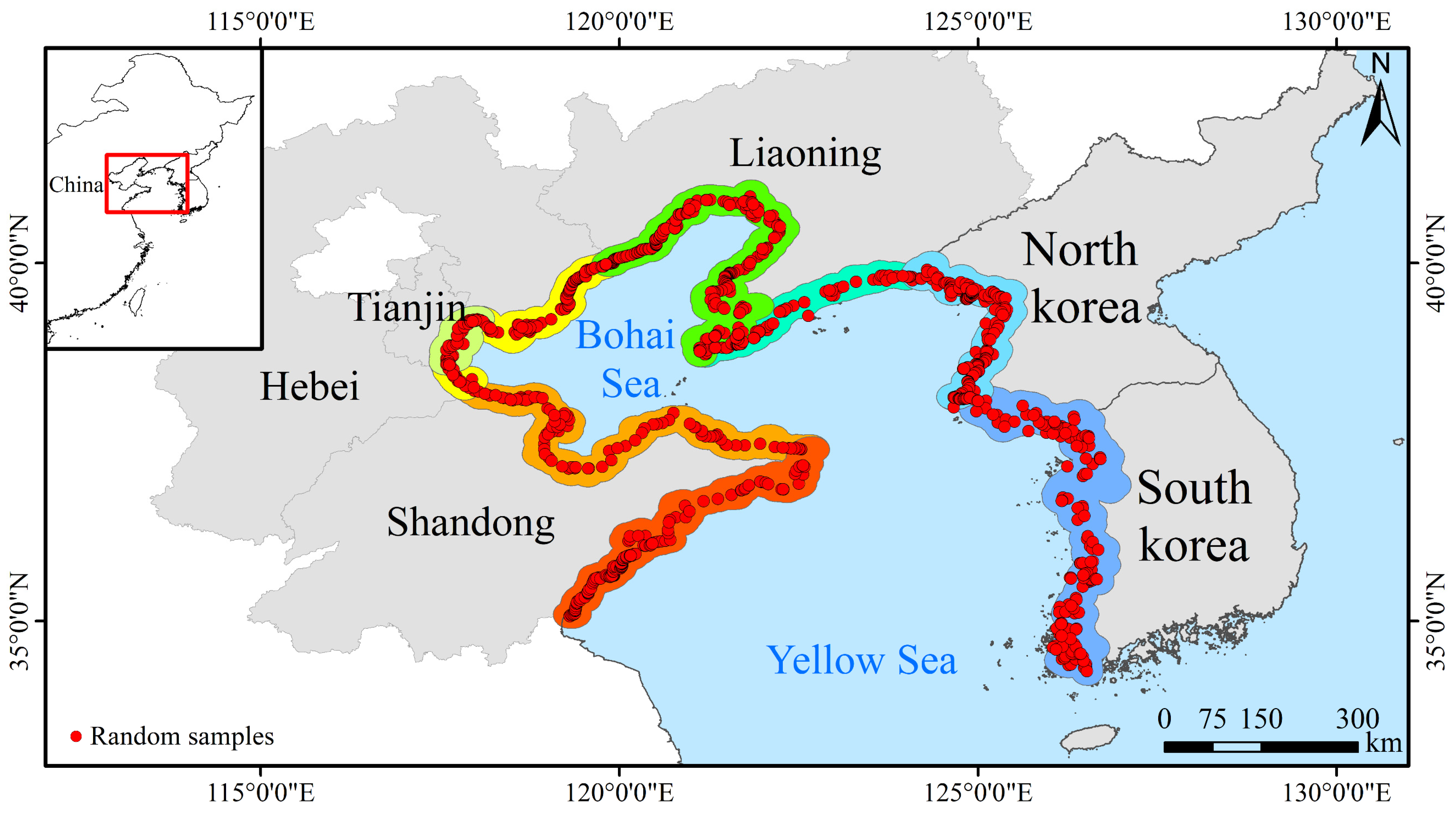
2.1. Study Area

The study area spans the coastal regions around the Bohai and Yellow Seas, including the coast of one municipality (Tianjin) plus three provinces (Shandong, Hebei, and Liaoning) of China and the western coast of the Korean Peninsula. The western coast of the Korean Peninsula in this study starts from the Yalu River estuary to the south end of the Korean Peninsula. The whole region extends from 34.05°N to 41.25°N, which lies in a semi-humid temperate zone. Tidal wetland around the Bohai and Yellow Seas is up to 20 km in width and is mainly composed of tidal flats, which are among the most extensive on the earth [8,46]. Thus, taking the calculating efficiency into consideration, the study area was further confined within 20 km buffer of the coastline (Figure 1).

2.2. Datasets

2.2.1. Sentinel-1 Data

The Sentinel-1 mission includes two satellites (Sentinel-1A launched in Apr 2014 and Sentinel-1B launched in Apr 2016). The dual-polarization C-band SAR loaded on the mission produces high revisit frequency (6 day at the equator), all-weather, and all-time images [33,47]. The data were restricted to the Interferometric Wide Swath (IWS) mode, 10 m resolution, and VV polarized in this study [33]. Furthermore, intersected with a 1 km buffer of the study region coast, a total of 1342 Sentinel-1 images from 1 Oct 2020 to 31 Oct 2021 were selected.

2.2.2. Sentinel-2 Data

The Sentinel-2 mission comprises two identical satellites (Sentinel-2A and Sentinel-2B) running in a sun-synchronous orbit. After the launch of Sentinel-2B in March 2017, this mission could achieve a global 5-day revisit frequency. With their multispectral instruments, they provide sufficient wide-swath (290 km) and high-resolution (visible and NIR at 10 m) data for coastal area mapping [48].
The whole archive of open-access Sentinel-2 data in GEE platform has been thoroughly pre-processed, which makes it analysis-ready. The Level-2A surface reflectance imagery was applied in this study. To attenuate the impact of cloud contamination, taking advantage of the Sentinel-2 Quality Assessment 60 (QA) bitmask band that contains cloud information [49], images with cloud cover greater than 50% were firstly filtered out, and then pixels covered by opaque and cirrus clouds [50] in the filtered images were masked (Figure 2). The remaining pixels were considered good observations (Figure 1). To avoid unnecessary computing, the imagery was limited to scenes that intersected a 1 km buffer of the study region coastline. Finally, a total of 3477 images taken from 1 Oct 2020 to 31 Oct 2021 were available for further analysis.

2.2.3. Validation Samples
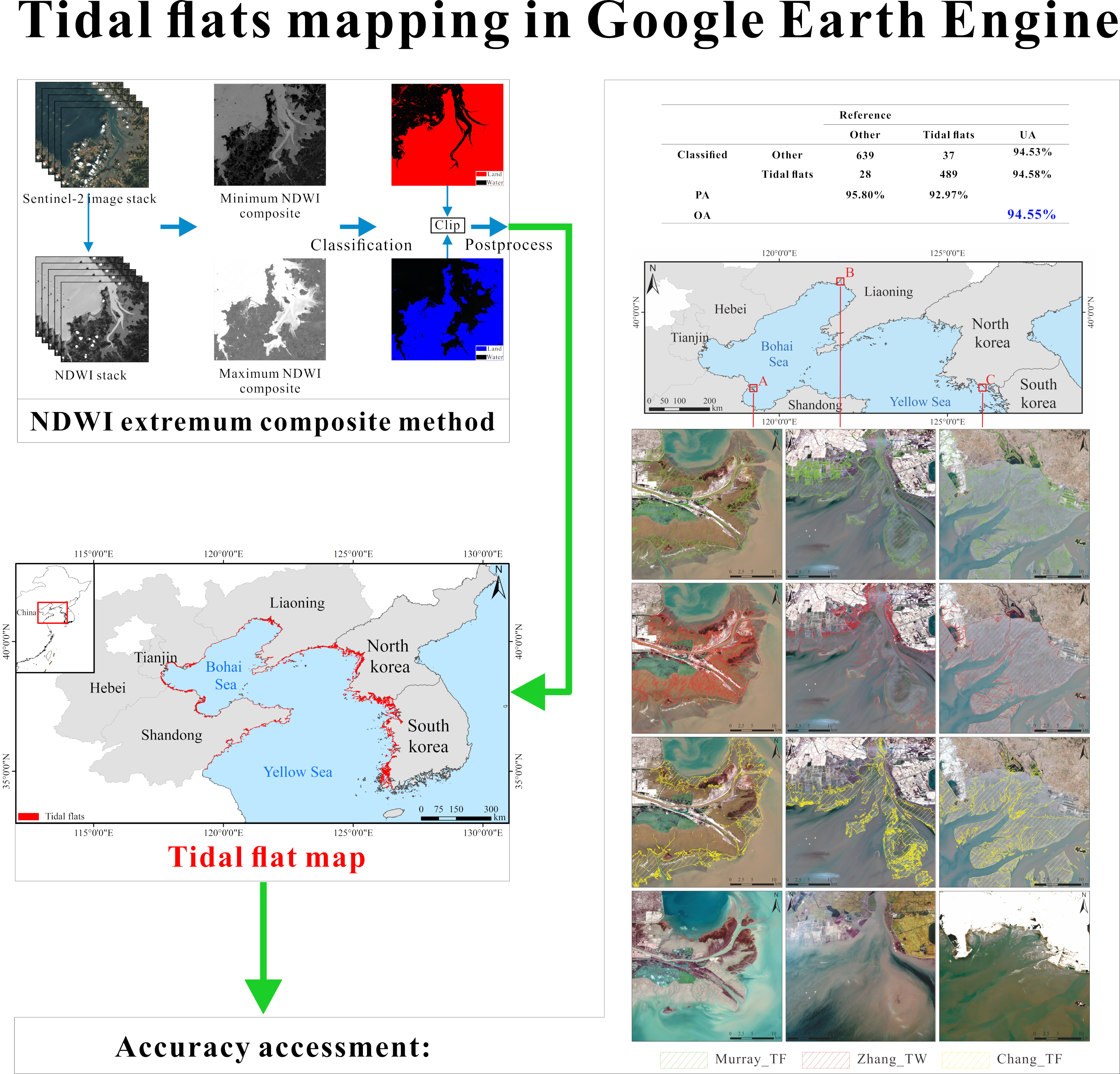
To evaluate the accuracy of the tidal flat map produced, an independent validation set of 1193 samples was randomly selected along the study area coast (Figure 3). All the samples were obtained based on very high spatial resolution images in Google Earth or low-tide Sentinel-2 images. Each sample was labeled as one of the two classes (tidal flat and other) according to visual inspection.

2.3. Methods

A simple, high-efficiency and robust tidal flat mapping algorithm was developed and has great potential to be applied to larger scales. Firstly, the cloud-masked Sentinel-2 imagery stack was composited to maximum and minimum NDWI image. Then, through adaptive classification method, the largest and smallest water extent were identified. Thus, the tidal flat ranges could be derived from smallest water extent subtracting largest water extent. Thirdly, we postprocessed the preliminary tidal flat maps, removing inland features and noise. Finally, the tidal flat map was validated in a quantitative and visual way. Additionally, we made attempts in SAR data tidal flat mapping using a similar technique flow for comparison.

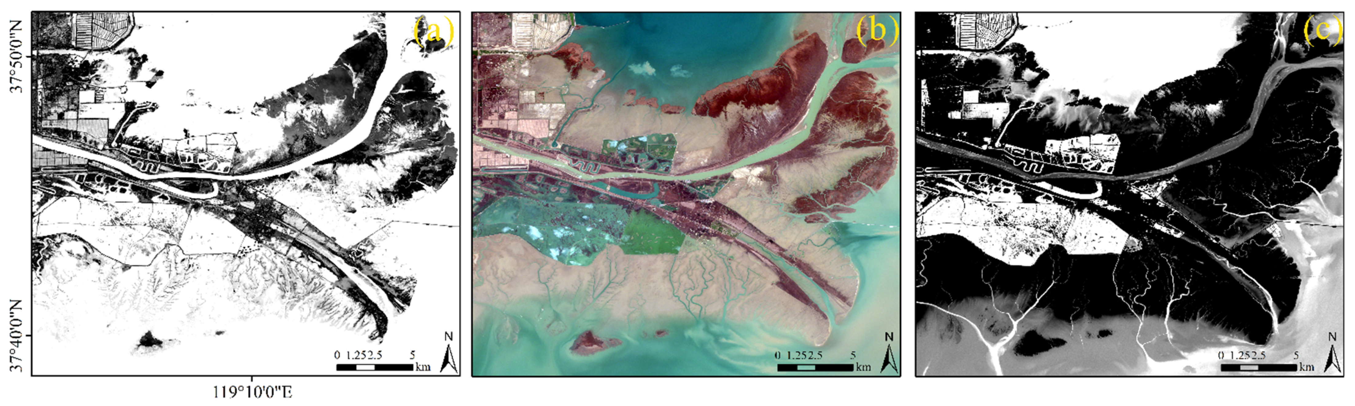
2.3.1. Maximum and Minimum Water Area Extraction

After the cloud masking, we calculated the NDWI [51] of every pixel in the image collection. The NDWI has been widely used to distinguish open surface water from other features across different sensors, such as Landsat [8,27], and Sentinel-2 [10]. Although the NDWI may not be very sensitive to water with vegetation within one scene, the deciduous nature of the vegetation in the study area combined with the following mentioned compositing method could permit an effective mitigation. The NDWI is defined as:
NDWI = ρ g r e e n ρ N I R ρ g r e e n + ρ N I R                    
where ρ g r e e n is the reflectance of the green band (Band 3 of Sentinel-2 images), and ρ N I R is the reflectance of the near-infrared band (Band 8 of Sentinel-2 images).
Because of the fluctuating nature of tide, one tidal flat pixel could be identified as two classes (tidal flats and water) within a complete tide cycle. To determine the range of tide fluctuation, we applied the NDWI extremum composite method to the Sentinel-2 image stack. The extremum includes two ends: the maximum and minimum. In an image stack, the NDWI of the location of one certain pixel varies with tide cycles, with higher NDWI corresponding to water and lower to land. If this location had ever been submerged in water, then the maximal NDWI could capture this signal. We extract the maximal NDWI of all pixel locations in image stacks to produce the maximal NDWI composite image (Figure 2). Therefore, the maximal NDWI composite image represents the largest water extent [4,10]. Since coastal vegetation that is not submerged by water would be classified as land in the NDWI composites, the largest water extent images do not contain coastal vegetation. In contrast, if that location had ever been exposed above the sea surface, the minimal NDWI could also record it. As a result, the minimal NDWI composite image delineates the smallest water extent [10].

2.3.2. Identifying Land and Water Features

Based on proper threshold, land and water features in NDWI images could be efficiently segmented. Through the histogram of imagery, the Otsu method [52] could automatically identify the optimal threshold to divide imagery into two categories, which has been extensively used in previous studies [4,33,53,54,55]. The basic logic of the Otsu method is to maximize inter-class variance (the intra-class variance is minimized at the same time), during which the optimal threshold could be determined. The equation:
η ( k * ) = max 1 k n ω 0 ( k ) ω 1 ( k ) [ μ 0 ( k ) μ 1 ( k ) ] 2 δ 2
where k * represents the optimal threshold, k is one threshold, n is the grey level a pixel being presented. ω 0 ( k ) and ω 1 ( k ) are the possibilities of two categories based on k , whereas μ 0 ( k ) and μ 1 ( k ) are the means. δ 2 is the total variance.
The study area is divided into eight sub-regions based on the administrative boundary and geological positions (Figure 3). The sub-regions obtained 16 NDWI extremum (maximum and minimum) composite images, to which we applied the Otsu method and manually adjusted thresholds in some images to achieve a best binary classification. Through clipping, the preliminary tidal flat map (Figure 2) is available.

2.3.3. Post-Processing

The inland features and noises affect the accuracy of preliminary tidal flat map. Firstly, taking reference to the maximal water extent image derived from NDWI maximum composite, we adjusted the administrative boundary of the study region coast to make a high-tide coastline. The new adjusted coastline is the boundary between high tide and inland (Figure 4). Using this water–land boundary could mask out the inland features within the tidal flat map.
Secondly, using the “connectedPixelCount” function in GEE, small pixel groups that had less than 100 units were eliminated. Other larger noises were erased based on the Google Earth imagery.

2.3.4. Accuracy Assessment

The quality of land-cover maps is a basic feature of great significance to users [56]. A quantitative accuracy assessment was conducted using randomly selected validation samples along the study area coast. As for sample size planning, a commonly used sample size formula [56] was applied in this study:
n = z 2 p ( 1 p ) d 2
where n is the sample size, z equals 1.96 for a 95% confidence interval, d is the half-width of the confidence interval, and p is the desired overall accuracy in simple random sampling. In this case, when z is 1.96 (which means d equals to 0.05) and p is set to 0.80, then n equals to 246. The upper bound from this formula is achieved when p is 0.50, and, in our case, n is 384. Therefore, the 1193 samples generated in this study would be sufficient for the accuracy assessment. The samples were assigned to one of the two classes: ‘tidal flats’ or ‘other’ with a number of 526 and 667, respectively.
The confusion matrix was calculated, including three metrics: producer’s accuracy (PA), user’s accuracy (UA), and overall accuracy (OA) [57]. PA is the probability of one ground feature class being correctly classified by the land-cover map, quantifying omission errors. UA measures the probability of one classification result being consistent with the reality, quantifying commission errors. OA is the proportion of all correctly classified samples.

3. Results

3.1. Confusion Matrix

Through the NDWI extremum composite method, a 10 m resolution tidal flat map circa 2021 around the Bohai and Yellow Seas was generated. The OA of the tidal flat map is 94.55% with both UA and PA of ‘tidal flat’ and ‘other’ exceeding 92% (Table 1), suggesting good credibility of our results.

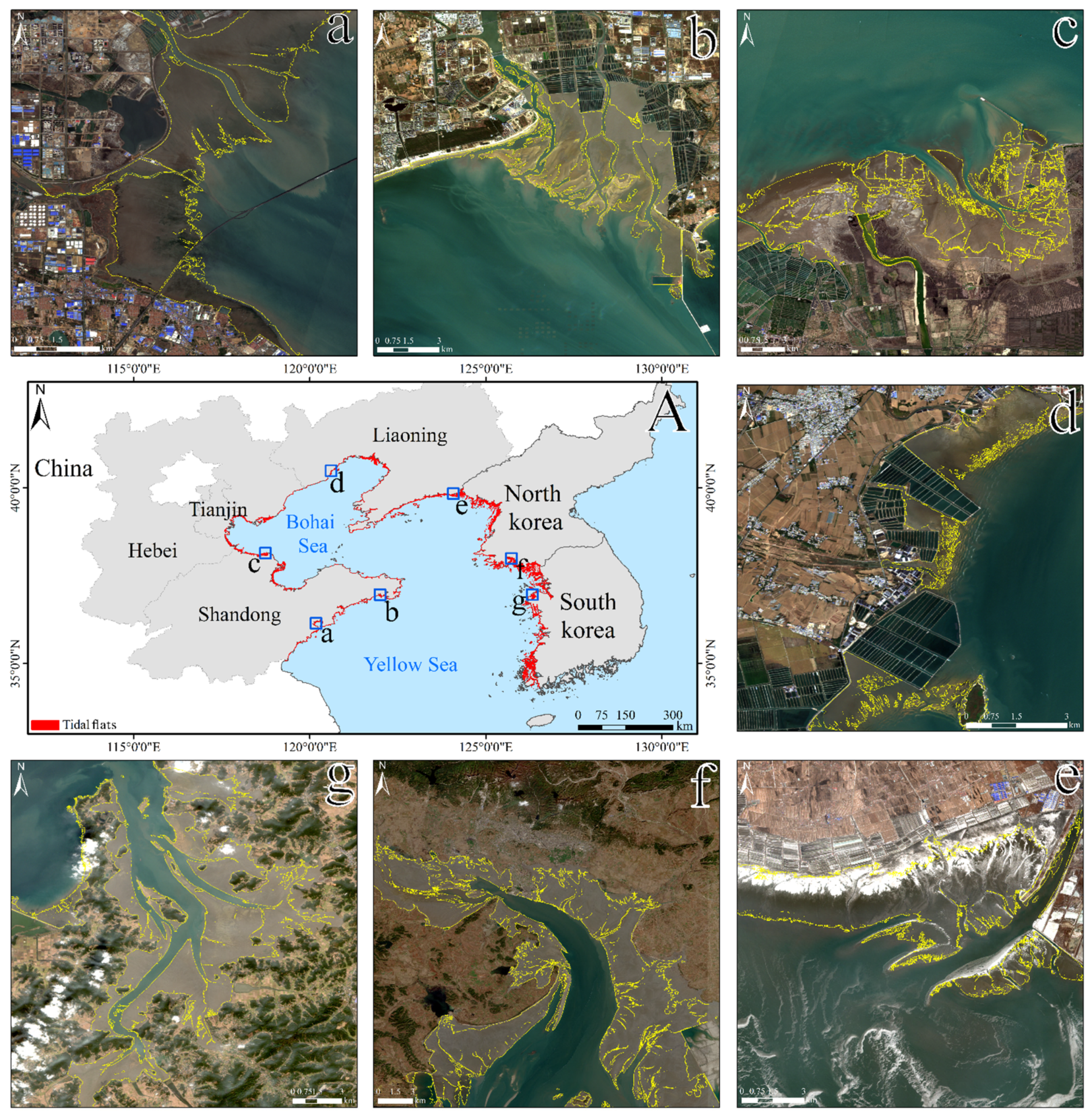
3.2. Spatial Distribution

The total tidal flats area around the Bohai and Yellow Seas is 546,360.2 ha, which is mostly distributed in the Korean Peninsula, Shandong, and Liaoning province (Figure 5). The tidal flats in the Korean Peninsula account for the largest proportion with an area of 342,559.7 ha. In the study area within China, Shandong province has the largest area of tidal flats (86,344.3 ha), followed by Liaoning province (80,633.8 ha). Hebei province holds an area of 29,462.4 ha. Tianjin municipality ranks last with 7360.0 ha. Most tidal flats were found around natural coasts, such as deltas, estuaries, coastal bays, and low-elevation flat areas (Figure 6), whereas artificial coasts, e.g., aquaculture ponds, coastal dams, and ports, usually barely hold tidal flats.
To display the tidal flats around the Bohai and Yellow seas intuitively, the tidal flats map was overlaid on the administrative boundary and Sentinel-2 lowest tide images (Figure 6). The lowest tide images during Oct 2020 to Oct 2021 were selected on the GEE platform. With the help of a filter function integrated in GEE, all time-relative and geolocation-relative images were stacked in image collections and visually checked to find the lowest tide images. As illustrated in Figure 6, the outline and shape of our tidal flat map achieved strong agreement with the lowest tide images. It should be noted that the turbid water clearly presented in Figure 6a–c,e was not wrongly classified as tidal flats. Additionally, in Figure 6b,c,e, the tidal flat map did not cover the entire area of those outside the artificial boundaries. That is because they were not inundated by sea water during the study period, although the geological features of those areas are similar to tidal flats.

4. Discussion

4.1. Practicability

Based on the GEE platform, this study mapped the tidal flat around the Bohai and Yellow Seas using NDWI extremum composite method and time series Sentinel-2 images. To our best knowledge, the proposed 10 m-resolution tidal flat map is currently the most updated around the Bohai and Yellow Seas. The abundant satellite data of the Sentinel-2 mission, the concise and reliable algorithm, the ability of one large area mapping per time, and the planetary-scale geospatial analysis platform GEE contribute to the practicality of the proposed tidal flat mapping method.
The key to mapping tidal flats is to obtain the images during the lowest tide and highest tide. Although the datasets of Landsat series have increased substantially with the launch of Landsat-8 [58,59], the 16-day or even longer revisit cycle means the massive observation omission of local tide conditions. Meanwhile, the globally 5-day revisit cycle of the Sentinel-2 mission has greatly increased the observation density, which means a higher availability of images close to extreme tide levels. Especially when it comes to the coast of China, Sentinel-2 is three times the observation frequency of Landsat series [4]. Furthermore, the 10 m resolution of Sentinel-2 could map tidal flats with more details, which is particularly practical in delineating narrow and scattered ones [60].
Secondly, our algorithm is easy to be reproduced and does not require tidal information. The logic of the NDWI extremum composite method is clear and simple: tidal flats equal maximum land extent (lowest tide) minus minimum land extent (highest tide). No large volume of training samples was needed in this process, which gives this method good versatility in all kinds of areas, especially when prior knowledge is lacking. Since the land–water boundary to eliminate the inland features was created based on the administrative boundaries, only areas that own newly constructed structures require to be adapted. The method of manually delineated coastline was also adopted in previous studies [26,55,61,62]. Tidal information could be available through in situ tidal stations and modelled tide level results. The tide height could be labeled on scenes to select the highest and lowest tide images. However, within one scene, mixed tide patterns, within-scene tidal variations, and inaccurately modelled tide could inevitably lead to errors in tidal flat mapping. On the contrary, the NDWI extremum composite method is pixel-based. Each pixel is selected from multiple same-location pixels in different images. The NDWI extremum composite image is the composition of all pixels that represent the maximum or minimum value of NDWI in the image stack. Thus, the necessity and uncertainty of tidal information could be averted.
Thirdly, the study area was divided into eight sub-regions (Figure 3). The principle of the division was based on geological position and administrative divisions. For example, tidal mapping in the long coast of Shandong and Liaoning will exceed the limits of memory and computation time of GEE, so we divided them into four parts at the east-most point of Shandong province and the south-most point of Liaoning province, respectively. The same reason was applied for the Korea Peninsula, whereas the two sub-regions in Hebei province and Tianjin municipality followed the administrative boundary. Previous studies used one image tile [2], 1 ° × 1 ° cells [33] or three image tiles [10] as the smallest computing unit. A small computing unit means a binary threshold that fits the local area, whereas our practice shows that it is also feasible to use a binary threshold on a large scale (Section 3). This is because the NDWI of land (permanent land and tidal flats) differs greatly from that of water, which gives the threshold of large areas some room for maneuver. In other words, although the threshold differences exist in different small areas, one single threshold is still competent for NDWI binary classification.
Fourthly, the cloud-based analysis platform GEE is significant in facilitating the processing of Sentinel-2 imagery. It archives large stacks of analysis-ready Sentinel-2 data and provides abundant tools for image processing in a parallel way. Moreover, the massive computing power enables GEE to analyze trillions of pixels in parallel theoretically [1,36].

4.2. Noises and Limitations

The extremum composite method would inevitably introduce noises into the composite image [10], particularly in the NDWI minimum composite. This is because water has higher NDWI value than other features in most cases. Therefore, if there has been other interference at sea, it is highly likely that this interference will appear in the NDWI minimum composite image as the lowest NDWI value in the image stack. However, the highest NDWI value at that location would still belong to sea water, meaning that the NDWI maximum composite image will not change.
Noises are composed of five types, including turbid water, anchored and moored ships, laver grids, cloud contamination, and other random noises. Water with high turbidity has lower NDWI value than common seawater; thus, turbid water could not be completely separated from tidal flats in some cases. Once a ship was captured in Sentinel-2 images, whether it was at anchorage or in port (eventually it would navigate to other areas), the much lower NDWI value of ships than ambient water would make the shape of this ship appear on the NDWI minimum composite but not on the maximum composite, which would misclassify this ship as tidal flats. The reason for laver grids is not the same: laver grids float on the sea and could be submerged under waves, and this fluctuation nature also leads to misclassification. Next, although we masked cloud and cloud shadow using the QA band of Sentinel-2 imagery, omission errors still existed in some regions [63], meaning the presence of cloud contamination noises. The fifth kind of noises, namely random noises, are mainly spectral outliers.
Besides noises, there are still some intrinsic limitations that would impair the quality of tidal flat maps. Note that sun-synchronous satellites such as Sentinel-2 can only observe a portion of the astronomical tide range [64]; the tidal flat map in this study was restricted to “observed tidal range” [1], rather than the full tide range in reality. In addition, the 10 m resolution (in visible and NIR band) of Setninel-2 mission could still produce mixed pixels and create coarse tidal flats edges in some areas.

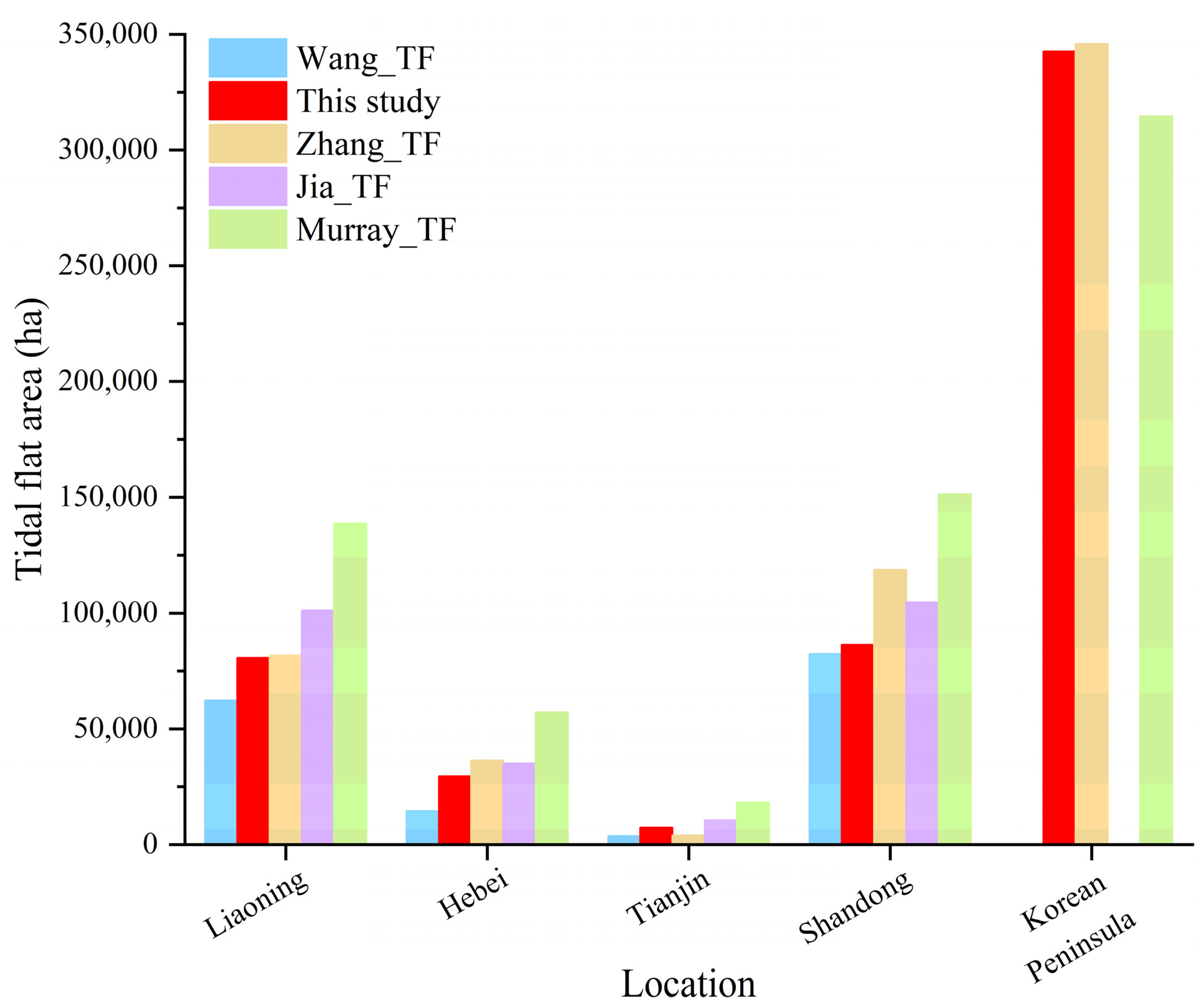
4.3. Comparisions with Other Results

The area [1,4,10,26] and spatial distribution [1,10] of several tidal flat products were collected for comparison with this study (Figure 7 and Figure 8): global distribution of tidal flat map data circa 2015 [1] (hereinafter referred to as Murray_TF), China tidal flat map circa 2019 [4] (hereinafter referred to as Jia_TF), coastal wetlands maps of China in 2018 [26] (hereinafter referred to as Wang_TF), and East Asia tidal wetland map circa 2020 [10] (hereinafter referred to as Zhang_TF). Clear differences exist in these tidal flat maps. In general, the area of our tidal flat map is larger than that of Wang_TF and smaller than those of Zhang_TF and Jia_TF. Murray_TF shows broader tidal flats than this study in Liaoning, Hebei, Tianjin, and Shandong, whereas in the Korea Peninsula, the situation is reversed.
Wang_TF used one-year Landsat data and set thresholds and relations of multiple spectral indices to identify tidal flats. Firstly, compared with 30 m-resolution Landsat data, the 10 m resolution of Sentinel-2 images could capture larger tidal flats, especially those narrow and patchy ones. Moreover, the availability of Sentinel-2 images (2–5 days revisit frequency) means Sentinel-2 imagery has more possibilities to map a larger extent of tidal flats than the combination of Landsat 7/8 (8–16 days revisit frequency). Secondly, Wang_TF tended to misclassify the most seaward tidal flats as parament water [26]. The aforementioned two reasons contributed to its smaller area than our results. As for Zhang_TF, the main reason for the inconsistency is the different mapping algorithm. Zhang_TF applied the random forest method [65] in terms of tidal flats and water classification. The tidal flats in this study are strictly defined as the mud or sand flats located between high tide line and low tide line. However, some mud or sand flats located above the high tide line have the same mineral composition as tidal flats; thus, they can be classified as tidal flats in the random forest method, but not in our results.
The larger tidal flat extent of Jia_TF than in our results could be mainly explained by the use of different spectral indexes. When determining the maximum water extent, Jia_TF chose mNDWI [66] maximum composite, whereas we used NDWI maximum composite. As illustrated in Figure 9, the mNDWI that is more sensitive to water [66,67,68] could regard moist soil as water [69]. Large portion of mud flats located above the highest tide line was regarded as water in the mNDWI composite (Figure 9a), whereas NDWI maximum composite (Figure 9c) showed high fidelity compared with the highest tide optical image (Figure 9b). In this way, Jia_TF enlarged the potential tidal flat range, which is the reason why the tidal flat area of Jia_TF is larger than ours.
The result of Murray_TF roughly represents the tidal flats condition of 2015, so differences were expected. However, the huge differences are unlikely to be attributed to the tidal flat evolution. Especially, evidence shows that there is rebound in China’s coastal wetland following restoration and conservation [70], which is contrary to the situation that Murray_TF (circa 2015) is generally much larger than our result (circa 2021). The generally larger tidal flat extent of Murray_TF has been studied in previous studies. As the soils of inland water area and aquaculture ponds could be exposed during dry periods, the random-forest-based Murray_TF could misclassify them as tidal flats [4,10,26,33]. Since the aquaculture ponds extensively spread over China coasts [15], this made the aforementioned factor the most important disparity source between Murray_TF and ours. Additionally, a portion of salt marshes and inland vegetation was also included in Murray_TF [4,10,33]. Nevertheless, the Korean Peninsula tidal flats in Murray_TF are smaller than in our results. The reasons for this are various. First of all, aquaculture ponds in the Korean Peninsula are less well-distributed than in China. Secondly, the predictor data layer that used in the random forest classifier of Murray_TF did not include the lowest tide images, which leads to the omission of lower tidal flats [10]. Finally, the 30 m resolution Landsat data Murray_TF used could also result in an incomplete tidal flat map.

4.4. Tidal Flats Mapping Using SAR Images

SAR images from Sentinel-1 mission could act as a useful complementary data source in tidal flat mapping for its unique advantages in data acquisition and data density. Using C-band Sentinel-1 SAR imagery, Zhao et al. [33] applied a quantile synthesis method in Southern China tidal flats mapping and achieved an overall accuracy of 92.4%. Generally, in SAR grayscale images, higher values are inclined to represent land, and lower values are more inclined to represent water. Therefore, the compositing of high and low values in time series SAR grayscale images would produce images that reflect low- and high-tide datum. The basic idea of quantile synthesis method is that, the difference of the 95th quantile (representing low tide datum) and the 5th quantile (representing high tidal datum) at each pixel location of Sentinel-1 grayscale images produces the tidal flat map. The choosing of the 95th and 5th quantiles instead of the largest and minimum ones is to avoid the relatively high speckle noises. Basically, the quantile synthesis method is similar to our NDWI extremum composite method. We implemented that method in several sites beyond Southern China to investigate its practicability in areas around the Bohai and Yellow Seas.
We postprocessed the preliminary quantile synthesis method results through noise and inland features removing. Compared to our results, tidal flats derived from SAR quantiles are much less in extent (Figure 8 and Figure 10) in three test locations. This may be attributed to the high sensitivity to water of C-band SAR data, which means some tidal flats saturated with water could be displayed as water in grayscale SAR images.
Nevertheless, the idea of extremum composite method used in SAR images still shows potential in tidal flats mapping. In the near future, the combination and fusion of optical and SAR imagery may serve tidal flats mapping better.

5. Conclusions

The unstable nature of tide has long made extensive area tidal flat mapping a great challenge to the scientific community. By taking the advantages of cloud computing platform GEE and high-density Sentinel-2 data archive, this study proposed a concise, accurate, and general tidal flat mapping algorithm (NDWI extremum composite method). This algorithm composited maximum and minimum NDWI at each pixel and used an adaptive classification method to produce the tidal flat map. The proposed method removed the inland features and overcame the dependence on tidal information and large sample datasets, which significantly reduce the necessity for prior knowledge of experts. Additionally, the quantile synthesis method using SAR imagery was also tested in the study area, and the tidal flat range obtained is much smaller than in our results.
The derived 10 m-resolution tidal flat map reveals the newest tidal flat extent around the Bohai and Yellow Seas. The overall accuracy of our approach achieved 94.55%. Visual inspection and comparison with existing products further suggest the reliability of our results, which indicate its potential use in global coastal ecosystem management, carbon neutrality, and sustainable development.

Author Contributions

Conceptualization, M.C., P.L. and Z.L.; methodology, M.C., P.L. and Z.L.; formal analysis and validation, M.C. and P.L.; investigation, M.C. and P.L.; resources, P.L. and Z.L.; writing—original draft preparation, M.C. and P.L.; writing—review and editing, M.C., P.L., Z.L. and H.W.; project administration, P.L., Z.L. and H.W.; data curation, M.C. and P.L.; visualization, M.C. and P.L.; supervision, P.L., Z.L. and H.W.; funding acquisition, P.L., Z.L. and H.W. All authors have read and agreed to the published version of the manuscript.

Funding

This work was jointly supported by the Natural Science Foundation of China (no. 42041005-4; no. 41806108), National Key Research and Development Program of China (no. 2017YFE0133500; no. 2016YFA0600903), Open Research Fund of State Key Laboratory of Estuarine and Coastal Research (no. SKLEC-KF202002) from East China Normal University, as well as State Key Laboratory of Geodesy and Earth’s Dynamics from Innovation Academy for Precision Measurement Science and Technology, Chinese Academy of Sciences (SKLGED2021-5-2). Z.H. Li was supported by the European Space Agency through the ESA-MOST DRAGON-5 Project (ref.: 59339).

Data Availability Statement

Sentinel-1 and Sentinel-2 datasets used in this study are publicly available online: https://scihub.copernicus.eu/dhus/#/home (accessed on 13 October 2021). The tidal flat maps are available from the corresponding author upon reasonable request.

Acknowledgments

We thank the Google Earth Engine platform and European Space Agency for the free-access Sentinel-1 and Sentinel-2 datasets. The authors sincerely thank all anonymous reviewers and the editors for their constructive and excellent reviews that have greatly improved the quality of the article.

Conflicts of Interest

The authors declare no conflict of interest.

References

  1. Murray, N.J.; Phinn, S.R.; DeWitt, M.; Ferrari, R.; Johnston, R.; Lyons, M.B.; Clinton, N.; Thau, D.; Fuller, R.A. The global distribution and trajectory of tidal flats. Nature 2019, 565, 222–225. [Google Scholar] [CrossRef] [PubMed]
  2. Zhang, K.; Dong, X.; Liu, Z.; Gao, W.; Hu, Z.; Wu, G. Mapping Tidal Flats with Landsat 8 Images and Google Earth Engine: A Case Study of the China’s Eastern Coastal Zone circa 2015. Remote Sens. 2019, 11, 924. [Google Scholar] [CrossRef] [Green Version]
  3. Wang, X.; Xiao, X.; Zou, Z.; Chen, B.; Ma, J.; Dong, J.; Doughty, R.B.; Zhong, Q.; Qin, Y.; Dai, S.; et al. Tracking annual changes of coastal tidal flats in China during 1986–2016 through analyses of Landsat images with Google Earth Engine. Remote Sens. Environ. 2020, 238, 110987. [Google Scholar] [CrossRef] [PubMed]
  4. Jia, M.; Wang, Z.; Mao, D.; Ren, C.; Wang, C.; Wang, Y. Rapid, robust, and automated mapping of tidal flats in China using time series Sentinel-2 images and Google Earth Engine. Remote Sens. Environ. 2021, 255, 112285. [Google Scholar] [CrossRef]
  5. Barbier, E.B.; Hacker, S.D.; Kennedy, C.; Koch, E.W.; Stier, A.C.; Silliman, B.R. The value of estuarine and coastal ecosystem services. Ecol. Monogr. 2011, 81, 169–193. [Google Scholar] [CrossRef]
  6. Ma, Z.; Melville, D.; Liu, J.; Chen, Y.; Yang, H.; Ren, W.; Zhang, Z.-W.; Piersma, T.; Li, B. Rethinking China’s new great wall. Science 2014, 346, 912–914. [Google Scholar] [CrossRef] [PubMed] [Green Version]
  7. Ghosh, S.; Mishra, D.R.; Gitelson, A.A. Long-term monitoring of biophysical characteristics of tidal wetlands in the northern Gulf of Mexico—A methodological approach using MODIS. Remote Sens. Environ. 2016, 173, 39–58. [Google Scholar] [CrossRef] [Green Version]
  8. Murray, N.J.; Clemens, R.S.; Phinn, S.R.; Possingham, H.P.; Fuller, R.A. Tracking the rapid loss of tidal wetlands in the Yellow Sea. Front. Ecol. Environ. 2014, 12, 267–272. [Google Scholar] [CrossRef] [Green Version]
  9. Bell, P.S.; Bird, C.O.; Plater, A.J. A temporal waterline approach to mapping intertidal areas using X-band marine radar. Coast. Eng. 2016, 107, 84–101. [Google Scholar] [CrossRef] [Green Version]
  10. Zhang, Z.; Xu, N.; Li, Y.; Li, Y. Sub-continental-scale mapping of tidal wetland composition for East Asia: A novel algorithm integrating satellite tide-level and phenological features. Remote Sens. Environ. 2022, 269, 112799. [Google Scholar] [CrossRef]
  11. Schuerch, M.; Spencer, T.; Temmerman, S.; Kirwan, M.L.; Wolff, C.; Lincke, D.; McOwen, C.J.; Pickering, M.D.; Reef, R.; Vafeidis, A.T.; et al. Future response of global coastal wetlands to sea-level rise. Nature 2018, 561, 231–234. [Google Scholar] [CrossRef]
  12. Nicholls Robert, J.; Cazenave, A. Sea-Level Rise and Its Impact on Coastal Zones. Science 2010, 328, 1517–1520. [Google Scholar] [CrossRef]
  13. Jasechko, S.; Perrone, D.; Seybold, H.; Fan, Y.; Kirchner, J.W. Groundwater level observations in 250,000 coastal US wells reveal scope of potential seawater intrusion. Nat. Commun. 2020, 11, 3229. [Google Scholar] [CrossRef]
  14. Sengupta, D.; Chen, R.; Meadows, M.E.; Choi, Y.R.; Banerjee, A.; Zilong, X. Mapping Trajectories of Coastal Land Reclamation in Nine Deltaic Megacities using Google Earth Engine. Remote Sens. 2019, 11, 2621. [Google Scholar] [CrossRef] [Green Version]
  15. Ren, C.; Wang, Z.; Zhang, Y.; Zhang, B.; Chen, L.; Xi, Y.; Xiao, X.; Doughty, R.B.; Liu, M.; Jia, M.; et al. Rapid expansion of coastal aquaculture ponds in China from Landsat observations during 1984–2016. Int. J. Appl. Earth Obs. Geoinf. 2019, 82, 101902. [Google Scholar] [CrossRef]
  16. Xu, N.; Gong, P. Significant coastline changes in China during 1991–2015 tracked by Landsat data. Sci. Bull. 2018, 63, 883–886. [Google Scholar] [CrossRef] [Green Version]
  17. McGranahan, G.; Balk, D.; Anderson, B. The rising tide: Assessing the risks of climate change and human settlements in low elevation coastal zones. Environ. Urban. 2007, 19, 17–37. [Google Scholar] [CrossRef]
  18. Tan, K.; Chen, J.; Zhang, W.; Liu, K.; Tao, P.; Cheng, X. Estimation of soil surface water contents for intertidal mudflats using a near-infrared long-range terrestrial laser scanner. ISPRS J. Photogramm. Remote Sens. 2020, 159, 129–139. [Google Scholar] [CrossRef]
  19. Campbell, A.; Wang, Y. Examining the Influence of Tidal Stage on Salt Marsh Mapping Using High-Spatial-Resolution Satellite Remote Sensing and Topobathymetric LiDAR. IEEE Trans. Geosci. Remote Sens. 2018, 56, 5169–5176. [Google Scholar] [CrossRef]
  20. Liu, Y.; Li, M.; Zhou, M.; Yang, K.; Mao, L. Quantitative Analysis of the Waterline Method for Topographical Mapping of Tidal Flats: A Case Study in the Dongsha Sandbank, China. Remote Sens. 2013, 5, 6138–6158. [Google Scholar] [CrossRef] [Green Version]
  21. Wei, W.; Tang, Z.; Dai, Z.; Lin, Y.; Ge, Z.; Gao, J. Variations in tidal flats of the Changjiang (Yangtze) estuary during 1950s–2010s: Future crisis and policy implication. Ocean Coast. Manag. 2015, 108, 89–96. [Google Scholar] [CrossRef]
  22. Tseng, K.; Kuo, C.; Lin, T.; Huang, Z.; Lin, Y.; Liao, W.; Chen, C. Reconstruction of time-varying tidal flat topography using optical remote sensing imageries. ISPRS J. Photogramm. Remote Sens. 2017, 131, 92–103. [Google Scholar] [CrossRef]
  23. Zhao, B.; Liu, Y.; Wang, L.; Liu, Y.; Sun, C.; Fagherazzi, S. Stability evaluation of tidal flats based on time-series satellite images: A case study of the Jiangsu central coast, China. Estuar. Coast. Shelf Sci. 2022, 264, 107697. [Google Scholar] [CrossRef]
  24. Dhanjal-Adams, K.L.; Hanson, J.O.; Murray, N.J.; Phinn, S.R.; Wingate, V.R.; Mustin, K.; Lee, J.R.; Allan, J.R.; Cappadonna, J.L.; Studds, C.E.; et al. The distribution and protection of intertidal habitats in Australia. Emu-Austral Ornithol. 2016, 116, 208–214. [Google Scholar] [CrossRef] [Green Version]
  25. Sagar, S.; Roberts, D.; Bala, B.; Lymburner, L. Extracting the intertidal extent and topography of the Australian coastline from a 28 year time series of Landsat observations. Remote Sens. Environ. 2017, 195, 153–169. [Google Scholar] [CrossRef]
  26. Wang, X.; Xiao, X.; Zou, Z.; Hou, L.; Qin, Y.; Dong, J.; Doughty, R.B.; Chen, B.; Zhang, X.; Chen, Y.; et al. Mapping coastal wetlands of China using time series Landsat images in 2018 and Google Earth Engine. ISPRS J. Photogramm. Remote Sens. 2020, 163, 312–326. [Google Scholar] [CrossRef]
  27. Murray, N.J.; Phinn, S.R.; Clemens, R.S.; Roelfsema, C.M.; Fuller, R.A. Continental Scale Mapping of Tidal Flats across East Asia Using the Landsat Archive. Remote Sens. 2012, 4, 3417–3426. [Google Scholar] [CrossRef] [Green Version]
  28. Chen, Y.; Dong, J.; Xiao, X.; Zhang, M.; Tian, B.; Zhou, Y.; Li, B.; Ma, Z. Land claim and loss of tidal flats in the Yangtze Estuary. Sci. Rep. 2016, 6, 24018. [Google Scholar] [CrossRef]
  29. Gu, J.; Jin, R.; Chen, G.; Ye, Z.; Li, Q.; Wang, H.; Li, D.; Christakos, G.; Agusti, S.; Duarte, C.M.; et al. Areal Extent, Species Composition, and Spatial Distribution of Coastal Saltmarshes in China. IEEE J. Sel. Top. Appl. Earth Obs. Remote Sens. 2021, 14, 7085–7094. [Google Scholar] [CrossRef]
  30. Han, Q.; Niu, Z. Remote-sensing monitoring and analysis of China intertidal zone changes based on tidal correction. Chin. Sci. Bull. 2018, 64, 456–473. [Google Scholar] [CrossRef] [Green Version]
  31. Fitton, J.M.; Rennie, A.F.; Hansom, J.D.; Muir, F.M.E. Remotely sensed mapping of the intertidal zone: A Sentinel-2 and Google Earth Engine methodology. Remote Sens. Appl. Soc. Environ. 2021, 22, 100499. [Google Scholar] [CrossRef]
  32. Turner, J.F.; Iliffe, J.C.; Ziebart, M.K.; Jones, C. Global Ocean Tide Models: Assessment and Use within a Surface Model of Lowest Astronomical Tide. Mar. Geod. 2013, 36, 123–137. [Google Scholar] [CrossRef] [Green Version]
  33. Zhao, C.; Qin, C.-Z.; Teng, J. Mapping large-area tidal flats without the dependence on tidal elevations: A case study of Southern China. ISPRS J. Photogramm. Remote Sens. 2020, 159, 256–270. [Google Scholar] [CrossRef]
  34. Wang, G.; Li, P.; Li, Z.; Ding, D.; Qiao, L.; Xu, J.; Li, G.; Wang, H. Coastal Dam Inundation Assessment for the Yellow River Delta: Measurements, Analysis and Scenario. Remote Sens. 2020, 12, 3658. [Google Scholar] [CrossRef]
  35. Zhang, H.; Jiang, Q.; Xu, J. Coastline Extraction Using Support Vector Machine from Remote Sensing Image. J. Multimed. 2013, 8, 175–182. [Google Scholar] [CrossRef]
  36. Gorelick, N.; Hancher, M.; Dixon, M.; Ilyushchenko, S.; Thau, D.; Moore, R. Google Earth Engine: Planetary-scale geospatial analysis for everyone. Remote Sens. Environ. 2017, 202, 18–27. [Google Scholar] [CrossRef]
  37. Pekel, J.-F.; Cottam, A.; Gorelick, N.; Belward, A.S. High-resolution mapping of global surface water and its long-term changes. Nature 2016, 540, 418–422. [Google Scholar] [CrossRef]
  38. Chen, S.; Woodcock, C.E.; Bullock, E.L.; Arévalo, P.; Torchinava, P.; Peng, S.; Olofsson, P. Monitoring temperate forest degradation on Google Earth Engine using Landsat time series analysis. Remote Sens. Environ. 2021, 265, 112648. [Google Scholar] [CrossRef]
  39. Mao, Y.; Harris, D.L.; Xie, Z.; Phinn, S. Efficient measurement of large-scale decadal shoreline change with increased accuracy in tide-dominated coastal environments with Google Earth Engine. ISPRS J. Photogramm. Remote Sens. 2021, 181, 385–399. [Google Scholar] [CrossRef]
  40. Zhang, X.; Xiao, X.; Qiu, S.; Xu, X.; Wang, X.; Chang, Q.; Wu, J.; Li, B. Quantifying latitudinal variation in land surface phenology of Spartina alterniflora saltmarshes across coastal wetlands in China by Landsat 7/8 and Sentinel-2 images. Remote Sens. Environ. 2022, 269, 112810. [Google Scholar] [CrossRef]
  41. Jin, X.; Xu, B.; Tang, Q. Fish assemblage structure in the East China Sea and southern Yellow Sea during autumn and spring. J. Fish Biol. 2003, 62, 1194–1205. [Google Scholar] [CrossRef]
  42. MacKinnon, J.; Verkuil, Y.I.; Murray, N. IUCN Situation Analysis on East and Southeast Asian Intertidal Habitats, with Particular Reference to the Yellow Sea (Including the Bohai Sea); International Union for the Conservation of Nature (IUCN): Gland, Switzerland, 2012; pp. 4–5. [Google Scholar]
  43. Murray, N.J.; Ma, Z.; Fuller, R.A. Tidal flats of the Yellow Sea: A review of ecosystem status and anthropogenic threats. Austral Ecol. 2015, 40, 472–481. [Google Scholar] [CrossRef]
  44. Yim, J.; Kwon, B.-O.; Nam, J.; Hwang, J.H.; Choi, K.; Khim, J.S. Analysis of forty years long changes in coastal land use and land cover of the Yellow Sea: The gains or losses in ecosystem services. Environ. Pollut. 2018, 241, 74–84. [Google Scholar] [CrossRef]
  45. Chen, Y.; Dong, J.; Xiao, X.; Ma, Z.; Tan, K.; Melville, D.; Li, B.; Lu, H.; Liu, J.; Liu, F. Effects of reclamation and natural changes on coastal wetlands bordering China’s Yellow Sea from 1984 to 2015. Land Degrad. Dev. 2019, 30, 1533–1544. [Google Scholar] [CrossRef]
  46. Wang, Y.; Zhu, D.; Wu, X. Chapter Thirteen Tidal flats and associated muddy coast of China. In Proceedings in Marine Science; Healy, T., Wang, Y., Healy, J.-A., Eds.; Elsevier: Amsterdam, The Netherlands, 2002; Volume 4, pp. 319–345. [Google Scholar]
  47. Lievens, H.; Reichle, R.H.; Liu, Q.; De Lannoy, G.J.M.; Dunbar, R.S.; Kim, S.B.; Das, N.N.; Cosh, M.; Walker, J.P.; Wagner, W. Joint Sentinel-1 and SMAP data assimilation to improve soil moisture estimates. Geophys. Res. Lett. 2017, 44, 6145–6153. [Google Scholar] [CrossRef] [PubMed]
  48. Drusch, M.; Del Bello, U.; Carlier, S.; Colin, O.; Fernandez, V.; Gascon, F.; Hoersch, B.; Isola, C.; Laberinti, P.; Martimort, P.; et al. Sentinel-2: ESA’s Optical High-Resolution Mission for GMES Operational Services. Remote Sens. Environ. 2012, 120, 25–36. [Google Scholar] [CrossRef]
  49. Zhu, Z.; Woodcock, C.E. Object-based cloud and cloud shadow detection in Landsat imagery. Remote Sens. Environ. 2012, 118, 83–94. [Google Scholar] [CrossRef]
  50. Li, H.; Jia, M.; Zhang, R.; Ren, Y.; Wen, X. Incorporating the Plant Phenological Trajectory into Mangrove Species Mapping with Dense Time Series Sentinel-2 Imagery and the Google Earth Engine Platform. Remote Sens. 2019, 11, 2479. [Google Scholar] [CrossRef] [Green Version]
  51. McFeeters, S.K. The use of the Normalized Difference Water Index (NDWI) in the delineation of open water features. Int. J. Remote Sens. 1996, 17, 1425–1432. [Google Scholar] [CrossRef]
  52. Otsu, N. A Threshold Selection Method from Gray-Level Histograms. IEEE Trans. Syst. Man Cybern. 1979, 9, 62–66. [Google Scholar] [CrossRef] [Green Version]
  53. Schlaffer, S.; Matgen, P.; Hollaus, M.; Wagner, W. Flood detection from multi-temporal SAR data using harmonic analysis and change detection. Int. J. Appl. Earth Obs. Geoinf. 2015, 38, 15–24. [Google Scholar] [CrossRef]
  54. Donchyts, G.; Baart, F.; Winsemius, H.; Gorelick, N.; Kwadijk, J.; van de Giesen, N. Earth’s surface water change over the past 30 years. Nat. Clim. Change 2016, 6, 810–813. [Google Scholar] [CrossRef]
  55. Zhu, Q.; Li, P.; Li, Z.; Pu, S.; Wu, X.; Bi, N.; Wang, H. Spatiotemporal Changes of Coastline over the Yellow River Delta in the Previous 40 Years with Optical and SAR Remote Sensing. Remote Sens. 2021, 13, 1940. [Google Scholar] [CrossRef]
  56. Stehman, S.V.; Foody, G.M. Key issues in rigorous accuracy assessment of land cover products. Remote Sens. Environ. 2019, 231, 111199. [Google Scholar] [CrossRef]
  57. Tu, C.; Li, P.; Li, Z.; Wang, H.; Yin, S.; Li, D.; Zhu, Q.; Chang, M.; Liu, J.; Wang, G. Synergetic Classification of Coastal Wetlands over the Yellow River Delta with GF-3 Full-Polarization SAR and Zhuhai-1 OHS Hyperspectral Remote Sensing. Remote Sens. 2021, 13, 4444. [Google Scholar] [CrossRef]
  58. Roy, D.P.; Wulder, M.A.; Loveland, T.R.; Woodcock, C.E.; Allen, R.G.; Anderson, M.C.; Helder, D.; Irons, J.R.; Johnson, D.M.; Kennedy, R.; et al. Landsat-8: Science and product vision for terrestrial global change research. Remote Sens. Environ. 2014, 145, 154–172. [Google Scholar] [CrossRef] [Green Version]
  59. Wulder, M.A.; Loveland, T.R.; Roy, D.P.; Crawford, C.J.; Masek, J.G.; Woodcock, C.E.; Allen, R.G.; Anderson, M.C.; Belward, A.S.; Cohen, W.B.; et al. Current status of Landsat program, science, and applications. Remote Sens. Environ. 2019, 225, 127–147. [Google Scholar] [CrossRef]
  60. Cao, W.; Zhou, Y.; Li, R.; Li, X. Mapping changes in coastlines and tidal flats in developing islands using the full time series of Landsat images. Remote Sens. Environ. 2020, 239, 111665. [Google Scholar] [CrossRef]
  61. Chen, B.; Xiao, X.; Li, X.; Pan, L.; Doughty, R.; Ma, J.; Dong, J.; Qin, Y.; Zhao, B.; Wu, Z.; et al. A mangrove forest map of China in 2015: Analysis of time series Landsat 7/8 and Sentinel-1A imagery in Google Earth Engine cloud computing platform. ISPRS J. Photogramm. Remote Sens. 2017, 131, 104–120. [Google Scholar] [CrossRef]
  62. Lopes, C.L.; Mendes, R.; Caçador, I.; Dias, J.M. Assessing salt marsh extent and condition changes with 35 years of Landsat imagery: Tagus Estuary case study. Remote Sens. Environ. 2020, 247, 111939. [Google Scholar] [CrossRef]
  63. Coluzzi, R.; Imbrenda, V.; Lanfredi, M.; Simoniello, T. A first assessment of the Sentinel-2 Level 1-C cloud mask product to support informed surface analyses. Remote Sens. Environ. 2018, 217, 426–443. [Google Scholar] [CrossRef]
  64. Bishop-Taylor, R.; Nanson, R.; Sagar, S.; Lymburner, L. Mapping Australia’s dynamic coastline at mean sea level using three decades of Landsat imagery. Remote Sens. Environ. 2021, 267, 112734. [Google Scholar] [CrossRef]
  65. Breiman, L. Random Forests. Mach. Learn. 2001, 45, 5–32. [Google Scholar] [CrossRef] [Green Version]
  66. Xu, H. Modification of normalised difference water index (NDWI) to enhance open water features in remotely sensed imagery. Int. J. Remote Sens. 2006, 27, 3025–3033. [Google Scholar] [CrossRef]
  67. Singh, K.V.; Setia, R.; Sahoo, S.; Prasad, A.; Pateriya, B. Evaluation of NDWI and MNDWI for assessment of waterlogging by integrating digital elevation model and groundwater level. Geocarto Int. 2015, 30, 650–661. [Google Scholar] [CrossRef]
  68. Wicaksono, A.; Wicaksono, P. Geometric accuracy assessment for shoreline derived from NDWI, MNDWI, and AWEI transformation on various coastal physical typology in Jepara Regency using Landsat 8 OLI imagery in 2018. Geoplan. J. Geomat. Plan. 2019, 6, 55–72. [Google Scholar] [CrossRef]
  69. Yang, Y.; Liu, Y.; Zhou, M.; Zhang, S.; Zhan, W.; Sun, C.; Duan, Y. Landsat 8 OLI image based terrestrial water extraction from heterogeneous backgrounds using a reflectance homogenization approach. Remote Sens. Environ. 2015, 171, 14–32. [Google Scholar] [CrossRef]
  70. Wang, X.; Xiao, X.; Xu, X.; Zou, Z.; Chen, B.; Qin, Y.; Zhang, X.; Dong, J.; Liu, D.; Pan, L.; et al. Rebound in China’s coastal wetlands following conservation and restoration. Nat. Sustain. 2021, 4, 1076–1083. [Google Scholar] [CrossRef]
Figure 1. Location of the study area and the spatial distribution of Sentinel-2 good observation number. The accurate range of good observation number is 23 to 334. The top left red circle denotes the study area on a broader scale.
Remotesensing 14 01789 g001
Figure 2. Workflow of tidal flat mapping in this study. TF: Tidal flats.
Remotesensing 14 01789 g002
Figure 3. Random selected samples along the study area coast. The 20 km buffer along the coast with different colors displays eight sub-regions that were delineated based on geological position and administrative divisions. The top-left red circle denotes the study area on a broader scale.
Remotesensing 14 01789 g003
Figure 4. Adjusted water–land boundary of different types (red line). (a) Aquaculture ponds; (b) coastal industrial area; (c) rocky coast; (d) estuaries. The underlying picture is the NDWI maximum composite image (in grey scale).
Remotesensing 14 01789 g004
Figure 5. Area statistics of tidal flats around the Bohai and Yellow Seas.
Remotesensing 14 01789 g005
Figure 6. Spatial distribution and areal extent of tidal flats around the coast of the Bohai and Yellow Seas (A). (a) Tidal flats in Jiaozhou bay, (b) tidal flats in Wuleidao bay; (c) tidal flats in Diaokou; (d) tidal flats in the Yantai River estuary; (e) tidal flats around Dandong port; (f) tidal flats in Haeju bay; and (g) tidal flats around Ho-ri, Korea. The yellow line in sub-figure a–g delineates the extent of tidal flats proposed by our method. Optical base maps used in sub-figure a–g are the true color Sentinel-2 images during the lowest tide, which were acquired at 02:58 on 21 Apr 2020, 02:48 on 20 Oct 2020, 03:07 on 14 Apr 2021, 02:57 on 18 Oct 2020, 02:47 on 7 Feb 2021, 02:37 on 17 Oct 2020, and 02:28 on 19 Oct 2020, respectively.
Remotesensing 14 01789 g006
Figure 7. Comparisons of tidal flat areas between our result (“This study”) and other results, including newest Murray_TF [1], Wang_TF [26], Jia_TF [4], and Zhang_TF [10].
Remotesensing 14 01789 g007
Figure 8. Exhibition of tidal flats range from the Murray_TF [1], our result (”This study”), and tidal wetlands range from Zhang_TW [10] in the Yellow river delta (region A), Liao Estuary (region B) and Haeju bay (region C), which are overlaid on the lowest-tide Sentinel-2 images acquired at 02:57 on 2 Mar 2021, 02:46 on 39 Mar 2021 and 02:37 on 17 Oct 2020, respectively. The last row represents the highest-tide Sentinel-2 images. From left to right, they are acquired at 02:57 on 10 Feb 2021, 02:47 on 10 Oct 2020 and 02:37 on 4 Feb 2021, respectively.
Remotesensing 14 01789 g008
Figure 9. Comparisons of (a) mNDWI maximum composite (in grey scale), (b) highest tide Sentinel-2 true color image acquired at 02:57 on 10 Feb 2021, and (c) NDWI maximum composite (in grey scale) in the Yellow River Delta.
Remotesensing 14 01789 g009
Figure 10. Case study results of quantile synthesis method through SAR imagery over the Yellow River Delta (the first row), Liao estuary (the second row), and Hajeu bay (the last row). The tidal flat maps were overlaid on 5th quantile images.
Remotesensing 14 01789 g010
Table 1. Confusion matrix of the proposed tidal flat map.
Reference
OtherTidal flatsUA
ClassifiedOther6393794.53%
Tidal flats2848994.58%
PA 95.80%92.97%
OA 94.55%
Publisher’s Note: MDPI stays neutral with regard to jurisdictional claims in published maps and institutional affiliations.

